Sampling, Sampling, Hypothesis & Hypothesis &

RegressionRegression

Sampling, Sampling, Hypothesis & Hypothesis &

RegressionRegression

TBS910 BUSINESS ANALYTICSTBS910 BUSINESS ANALYTICS

byProf. Stephen Ong

Visiting Professor, Shenzhen University

Visiting Fellow, Sydney Business School, University of Wollongong

Today’s Overview Today’s Overview

1.1. Using SamplesUsing Samples2.2. Hypothesis TestingHypothesis Testing3.3. RegressionRegression

TopicsTopics

7-3

USING SAMPLESUSING SAMPLES

1 - 4

Learning Objectives:Learning Objectives:

1.1. Understand how and why to use Understand how and why to use samplingsampling

2.2. Appreciate the aims of statistical Appreciate the aims of statistical inferenceinference

3.3. Use sampling distributions to find Use sampling distributions to find point estimates for population meanspoint estimates for population means

4.4. Calculate confidence intervals for Calculate confidence intervals for means and proportionsmeans and proportions

5.5. Use one-sided distributionsUse one-sided distributions6.6. Use Use tt-distributions for small samples-distributions for small samples

Collecting dataCollecting data

There are essentially two types of data There are essentially two types of data collectioncollection CensusCensus SampleSample

A census is often expensive, infeasible, A census is often expensive, infeasible, impossible, unnecessaryimpossible, unnecessary

The usual choice is to collect a sampleThe usual choice is to collect a sample

Sampling is the basis of Sampling is the basis of statistical inferencestatistical inference

This collects data from a random This collects data from a random sample of the populationsample of the population

Uses this data to estimates features of Uses this data to estimates features of the whole populationthe whole population

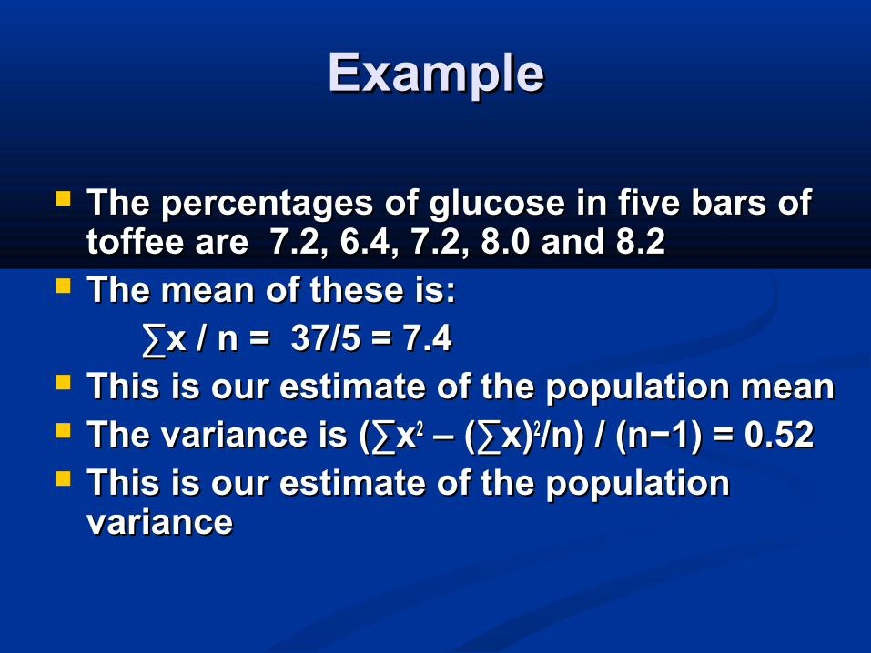
ExampleExample

The percentages of glucose in five bars of The percentages of glucose in five bars of toffee are 7.2, 6.4, 7.2, 8.0 and 8.2toffee are 7.2, 6.4, 7.2, 8.0 and 8.2

The mean of these is:The mean of these is:∑∑x / n = 37/5 = 7.4 x / n = 37/5 = 7.4

This is our estimate of the population meanThis is our estimate of the population mean The variance is (∑xThe variance is (∑x22 – (∑x) – (∑x)22/n) / (n/n) / (n−−1) = 0.52 1) = 0.52 This is our estimate of the population This is our estimate of the population

variancevariance

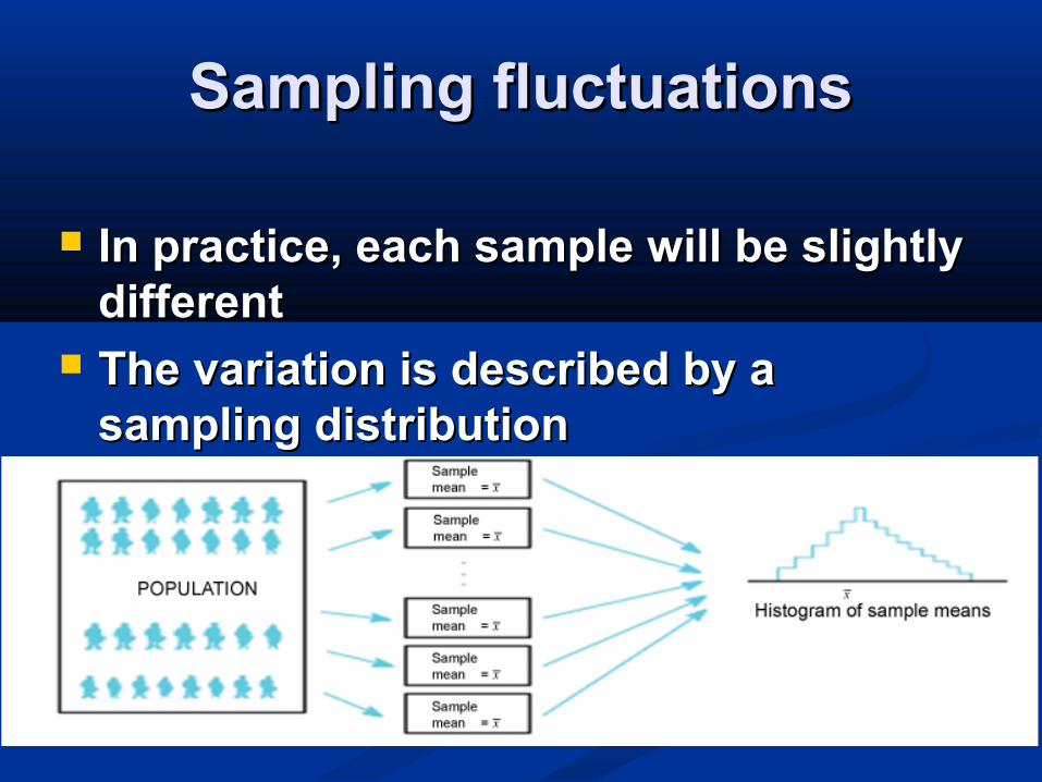
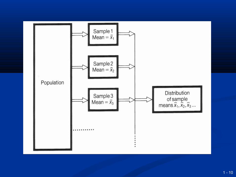
Sampling fluctuationsSampling fluctuations

In practice, each sample will be slightly In practice, each sample will be slightly different different

The variation is described by a The variation is described by a sampling distribution sampling distribution

1 - 10

Sampling distributionsSampling distributions

Data collected from samples gives a sampling Data collected from samples gives a sampling distribution, such as the sampling distribution distribution, such as the sampling distribution of the mean of the mean

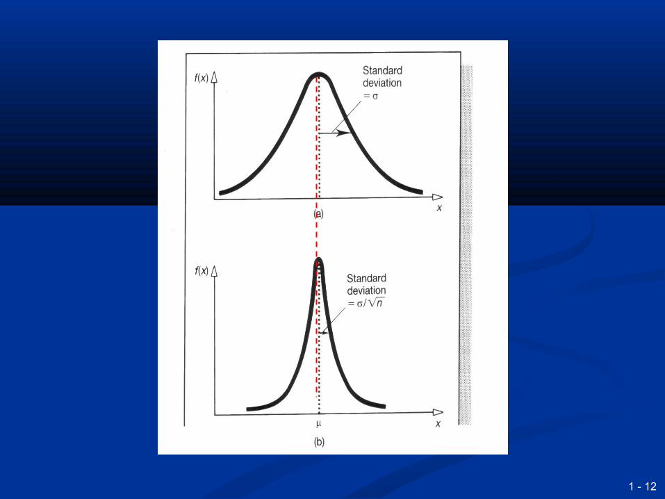
This has the features:This has the features: If a population is Normally distributed, the sampling If a population is Normally distributed, the sampling

distribution of the mean is also Normally distributed distribution of the mean is also Normally distributed With large samples the sampling distribution of the With large samples the sampling distribution of the

mean is Normally distributed regardless of the mean is Normally distributed regardless of the population distribution population distribution

The sampling distribution of the mean has a mean μ The sampling distribution of the mean has a mean μ and standard deviation σ/and standard deviation σ/√√nn

1 - 12

ExampleExample

Chocolate bars have a mean weight of 50g Chocolate bars have a mean weight of 50g and standard deviation of 10g. A sample of and standard deviation of 10g. A sample of 64 bars is taken and if the mean weight is 64 bars is taken and if the mean weight is less than 46g the whole days production is less than 46g the whole days production is scraped. scraped.

A large sample gives a sampling A large sample gives a sampling distribution with mean 50g and standard distribution with mean 50g and standard deviation 10/√64 = 1.25gdeviation 10/√64 = 1.25g

Z = (46Z = (46−−50)/1.25 = 50)/1.25 = −−3.23.2 P (Z< P (Z< −−3.2) = 3.2) = −−0.00070.0007

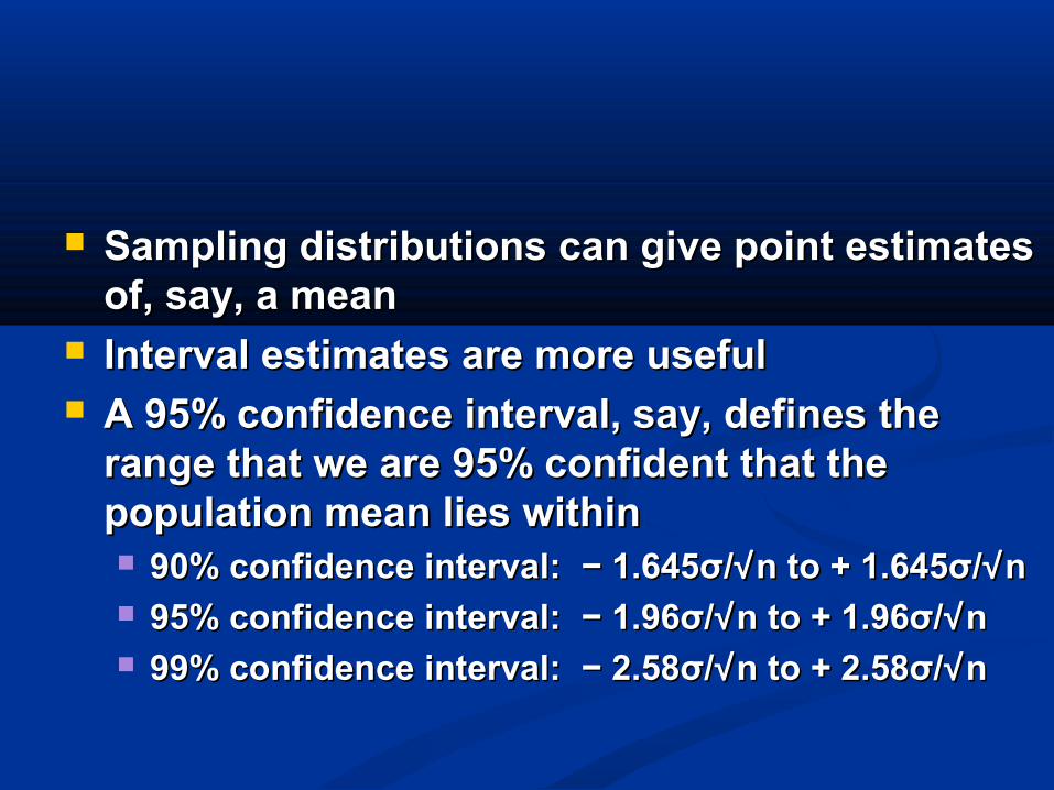
Sampling distributions can give point estimates Sampling distributions can give point estimates of, say, a meanof, say, a mean

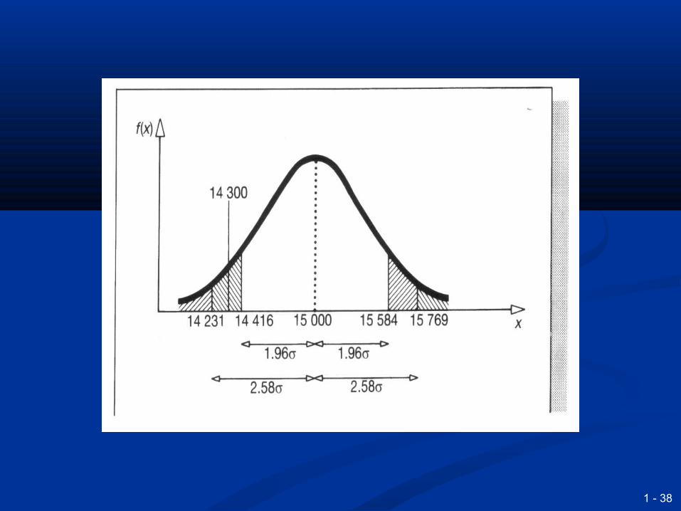
Interval estimates are more usefulInterval estimates are more useful A 95% confidence interval, say, defines the A 95% confidence interval, say, defines the

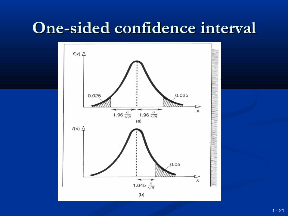
range that we are 95% confident that the range that we are 95% confident that the population mean lies withinpopulation mean lies within 90% confidence interval: 90% confidence interval: − − 1.645σ/1.645σ/√√n to + 1.645σ/n to + 1.645σ/√√ nn 95% confidence interval: 95% confidence interval: −− 1.96σ/ 1.96σ/√√n to + 1.96σ/n to + 1.96σ/√√nn 99% confidence interval: 99% confidence interval: −− 2.58σ/ 2.58σ/√√n to + 2.58σ/n to + 2.58σ/√√nn

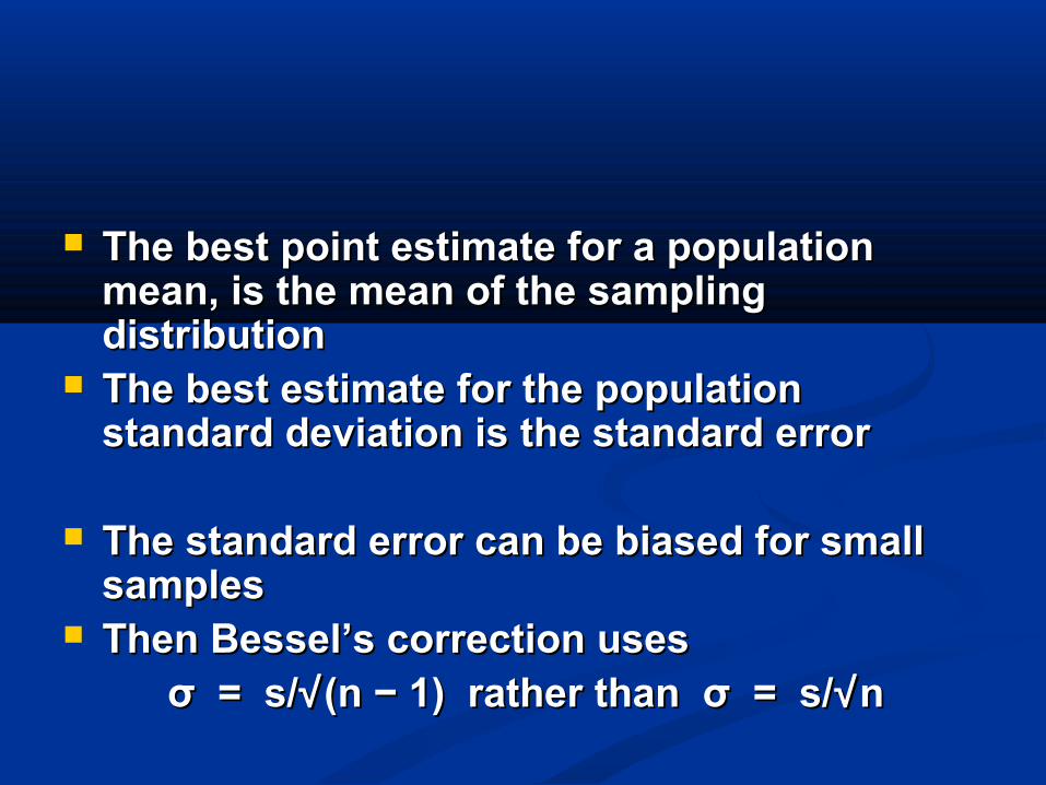
The best point estimate for a population The best point estimate for a population mean, is the mean of the sampling mean, is the mean of the sampling distributiondistribution

The best estimate for the population The best estimate for the population standard deviation is the standard errorstandard deviation is the standard error

The standard error can be biased for small The standard error can be biased for small samples samples

Then Bessel’s correction usesThen Bessel’s correction usesσ = s/σ = s/√√ (n (n −− 1) rather than σ = s/ 1) rather than σ = s/√√nn

1 - 16

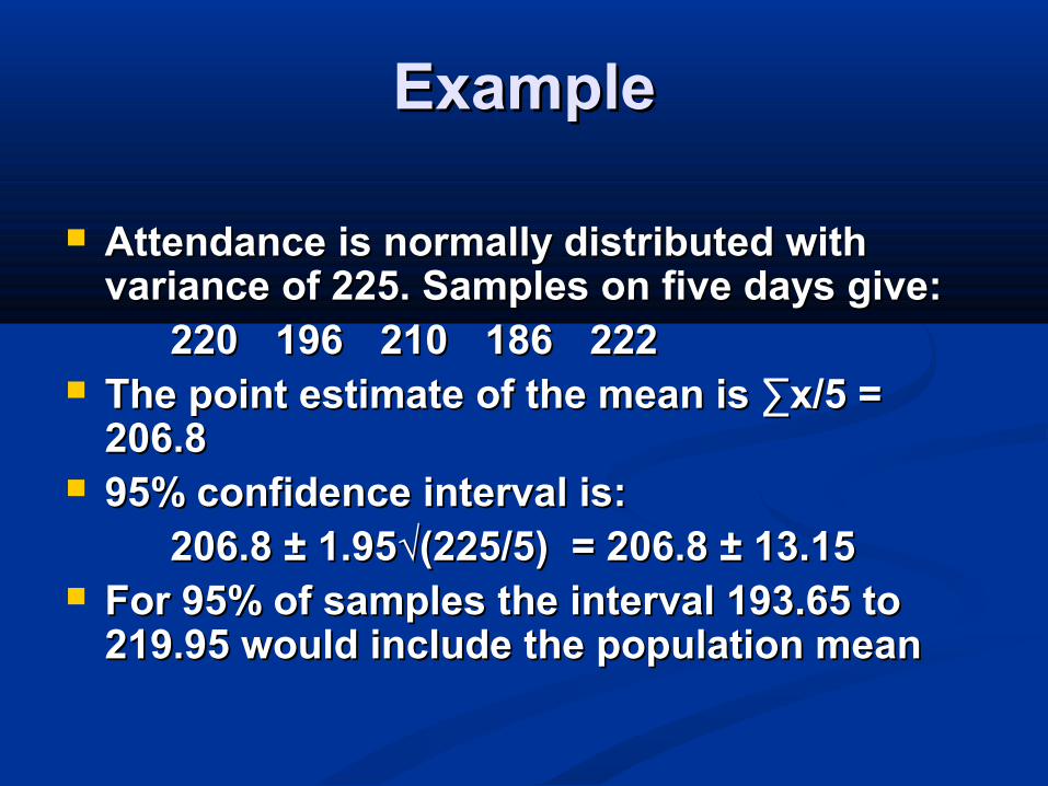
ExampleExample

Attendance is normally distributed with Attendance is normally distributed with variance of 225. Samples on five days give:variance of 225. Samples on five days give:

220220 196196 210210 186186 222222 The point estimate of the mean is ∑x/5 = The point estimate of the mean is ∑x/5 =

206.8206.8 95% confidence interval is:95% confidence interval is:

206.8 206.8 ± 1.95√(225/5) = 206.8 ± 13.15± 1.95√(225/5) = 206.8 ± 13.15 For 95% of samples the interval 193.65 to For 95% of samples the interval 193.65 to

219.95 would include the population mean219.95 would include the population mean

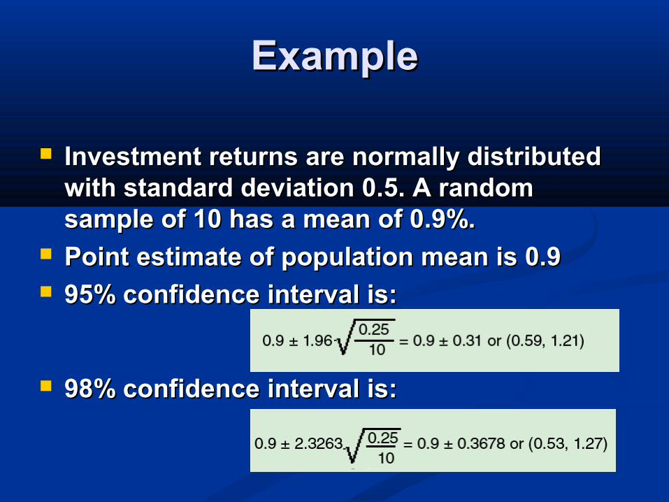
Investment returns are normally distributed Investment returns are normally distributed with standard deviation 0.5. A random with standard deviation 0.5. A random sample of 10 has a mean of 0.9%.sample of 10 has a mean of 0.9%.

Point estimate of population mean is 0.9Point estimate of population mean is 0.9 95% confidence interval is:95% confidence interval is:

98% confidence interval is:98% confidence interval is:

ExampleExample

The principles of sampling can The principles of sampling can be extended in many waysbe extended in many ways

Population proportions, where Population proportions, where sampling distributions are:sampling distributions are: Normally distributed Normally distributed with mean with mean ππ and standard deviation and standard deviation √√ ((ππ (1 (1 −− ππ )/n) )/n)

One sided confidence intervalsOne sided confidence intervals Small samplesSmall samples

Population proportionsPopulation proportions

With large sample (more than 30) the With large sample (more than 30) the sample proportions are:sample proportions are: Normally distributedNormally distributed with mean with mean ππ standard deviation standard deviation √√ ( (ππ (1 – (1 – ππ )/)/nn))

The 95% confidence interval is: The 95% confidence interval is: p – 1.96 p – 1.96 ×× √(p (1 √(p (1−−p) / n) p) / n)

to p + 1.96 to p + 1.96 ×× √(p (1 √(p (1 −− p) / n) p) / n)

1 - 21

One-sided confidence intervalOne-sided confidence interval

Sampling distributions with Sampling distributions with small samples are no longer small samples are no longer

NormalNormal Small samples tend to include fewer Small samples tend to include fewer

outlying values and under-estimate the outlying values and under-estimate the spreadspread

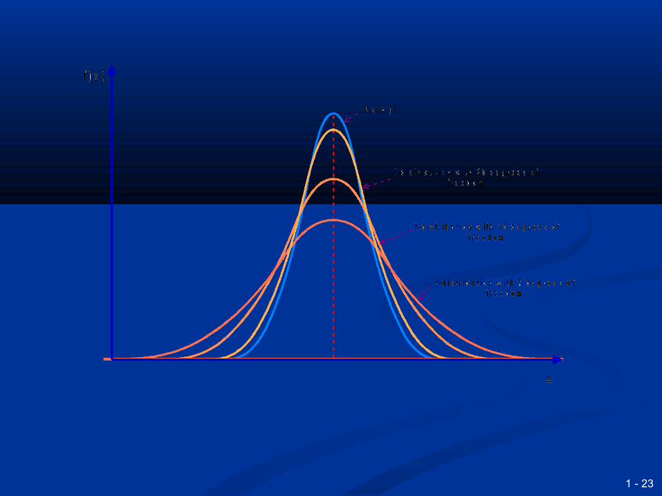
This effect is allowed for in t-This effect is allowed for in t-distributionsdistributions

The shape of the t-distribution depends The shape of the t-distribution depends on the degrees of freedomon the degrees of freedom

The degree of freedom is essentially The degree of freedom is essentially one less than the sample sizeone less than the sample size

1 - 23

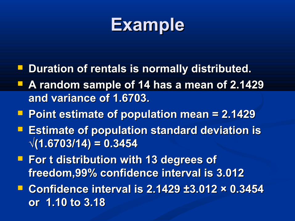
ExampleExample

Duration of rentals is normally distributed. Duration of rentals is normally distributed. A random sample of 14 has a mean of 2.1429 A random sample of 14 has a mean of 2.1429

and variance of 1.6703.and variance of 1.6703. Point estimate of population mean = 2.1429Point estimate of population mean = 2.1429 Estimate of population standard deviation is Estimate of population standard deviation is

√(1.6703/14) = 0.3454√(1.6703/14) = 0.3454 For t distribution with 13 degrees of For t distribution with 13 degrees of

freedom,99% confidence interval is 3.012freedom,99% confidence interval is 3.012 Confidence interval is 2.1429 Confidence interval is 2.1429 ±3.012 ±3.012 ×× 0.3454 0.3454

or 1.10 to 3.18or 1.10 to 3.18

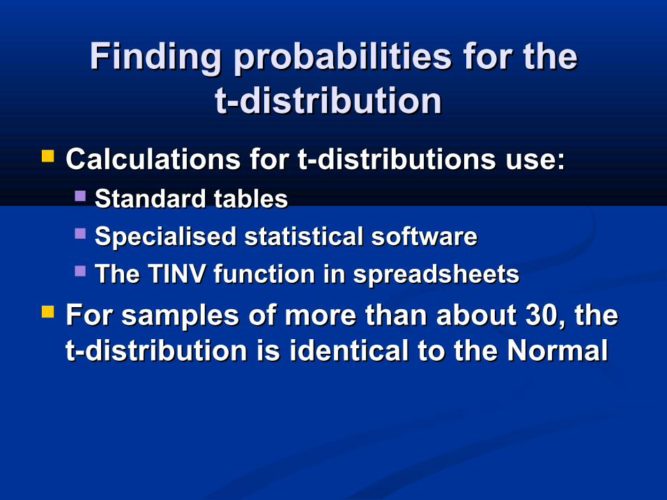
Finding probabilities for theFinding probabilities for thet-distribution t-distribution

Calculations for t-distributions use:Calculations for t-distributions use: Standard tables Standard tables Specialised statistical softwareSpecialised statistical software The TINV function in spreadsheetsThe TINV function in spreadsheets

For samples of more than about 30, theFor samples of more than about 30, thet-distribution is identical to the Normalt-distribution is identical to the Normal

1 - 26

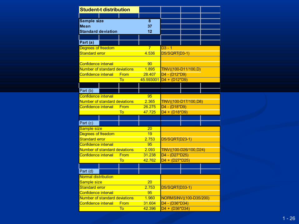
Student-t distribution

Sample size 8Mean 37Standard deviation 12

Part (a)Degrees of freedom 7 D3 - 1Standard error 4.536 D5/SQRT(D3-1)

Confidence interval 90Number of standard deviations 1.895 TINV((100-D11/100,D)Confidence interval From 28.407 D4 - (D12*D9)

To 45.593001 D4 + (D12*D9)

Part (b)Confidence interval 95Number of standard deviations 2.365 TINV((100-D17/100,D8)Confidence interval From 26.275 D4 - (D18*D9)

To 47.725 D4 + (D18*D9)

Part (c)Sample size 20Degrees of freedom 19Standard error 2.753 D5/SQRT(D23-1)Confidence interval 95Number of standard deviations 2.093 TINV((100-D26/100,D24)Confidence interval From 31.238 D4 - (D27*D25)

To 42.762 D4 + (D27*D25)

Part (d)Normal distributionSample size 20Standard error 2.753 D5/SQRT(D33-1)Confidence interval 95Number of standard deviations 1.960 NORMSINV((100-D35/200)Confidence interval From 31.604 D4 - (D36*D34)

To 42.396 D4 + (D36*D34)

TESTING HYPOTHESISTESTING HYPOTHESIS

1 - 27

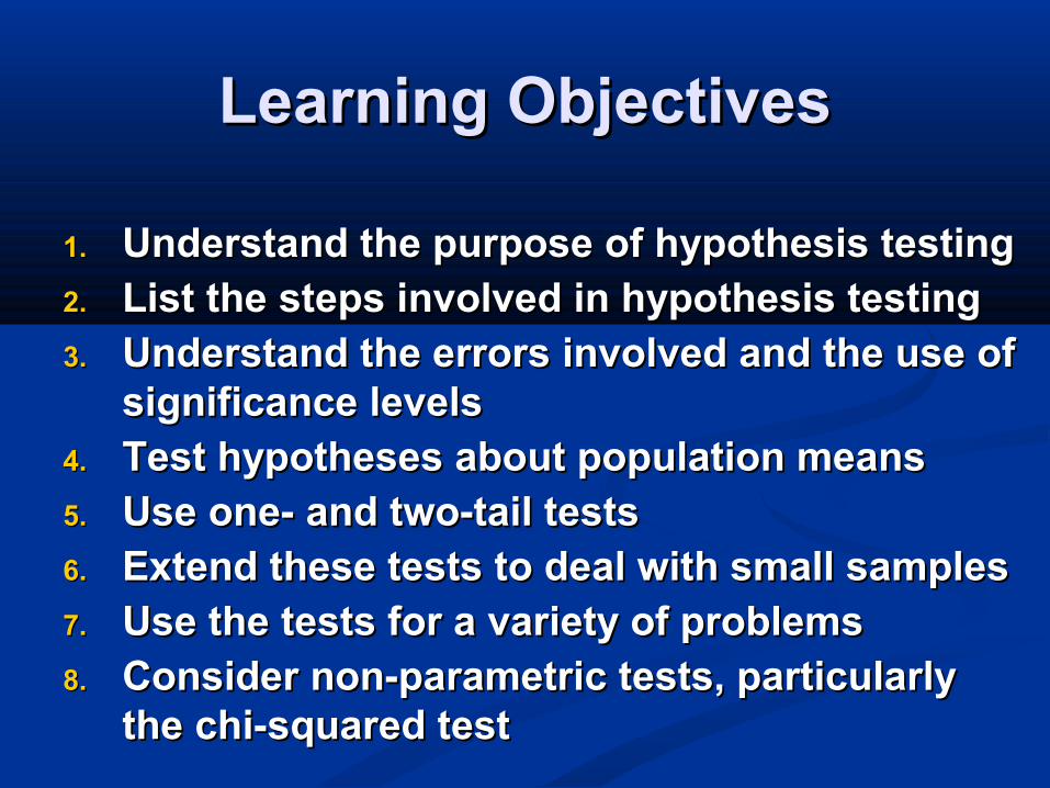
Learning ObjectivesLearning Objectives

1.1. Understand the purpose of hypothesis testingUnderstand the purpose of hypothesis testing2.2. List the steps involved in hypothesis testingList the steps involved in hypothesis testing3.3. Understand the errors involved and the use of Understand the errors involved and the use of

significance levelssignificance levels4.4. Test hypotheses about population meansTest hypotheses about population means5.5. Use one- and two-tail testsUse one- and two-tail tests6.6. Extend these tests to deal with small samplesExtend these tests to deal with small samples7.7. Use the tests for a variety of problemsUse the tests for a variety of problems8.8. Consider non-parametric tests, particularly Consider non-parametric tests, particularly

the chi-squared testthe chi-squared test

Hypothesis testingHypothesis testing

Considers a simple statement about a Considers a simple statement about a populationpopulation

This is the hypothesisThis is the hypothesis Uses a sample to test whether the statement is Uses a sample to test whether the statement is

likely to be true or is unlikelylikely to be true or is unlikely It sees whether or not data from a sample It sees whether or not data from a sample

supports a hypothesis about the populationsupports a hypothesis about the population If the hypothesis is unlikely, the hypothesis is If the hypothesis is unlikely, the hypothesis is

rejected and another implied hypothesis must rejected and another implied hypothesis must be truebe true

Define a simple, precise statement about Define a simple, precise statement about a population (the hypothesis)a population (the hypothesis)

Take a sample from the populationTake a sample from the population Test this sample to see if it supports the Test this sample to see if it supports the

hypothesis, or if it makes the hypothesis hypothesis, or if it makes the hypothesis highly improbablehighly improbable

If the hypothesis is highly improbable If the hypothesis is highly improbable reject it, otherwise accept itreject it, otherwise accept it

Procedure for hypothesis Procedure for hypothesis testingtesting

ExampleExample

A politician claims that 10% of factories A politician claims that 10% of factories in an area are losing money (hypothesis)in an area are losing money (hypothesis)

A sample of 30 shows that all of them are A sample of 30 shows that all of them are profitable (test statistic)profitable (test statistic)

If the hypothesis is true, the probabilityIf the hypothesis is true, the probabilitythat they are all profitable is 0.9that they are all profitable is 0.9 3030 = 0.0424 = 0.0424 (p-value)(p-value)

This is very unlikely, so we can reject the This is very unlikely, so we can reject the hypothesis (test result)hypothesis (test result)

Elements of a hypothesis testElements of a hypothesis test

1.1. Hypothesis – a simple statement Hypothesis – a simple statement about a populationabout a population

2.2. Test result - actual result from the Test result - actual result from the samplesample

3.3. Test statistic – a calculation about a Test statistic – a calculation about a sample assuming that the hypothesis sample assuming that the hypothesis is trueis true

4.4. Conclusion – either reject the Conclusion – either reject the hypothesis or nothypothesis or not

ExampleExample

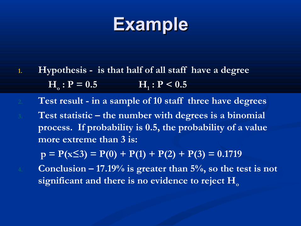
1. Hypothesis - is that half of all staff have a degree

Ho : P = 0.5 H1 : P < 0.5

2. Test result - in a sample of 10 staff three have degrees

3. Test statistic – the number with degrees is a binomial process. If probability is 0.5, the probability of a value more extreme than 3 is:

p = P(x≤3) = P(0) + P(1) + P(2) + P(3) = 0.1719

4. Conclusion – 17.19% is greater than 5%, so the test is not significant and there is no evidence to reject Ho

Because of uncertainty, we can Because of uncertainty, we can never be certain of the results never be certain of the results

Then we cannot really ‘accept’ a Then we cannot really ‘accept’ a hypothesis, but instead we say that we hypothesis, but instead we say that we ‘cannot reject’ it‘cannot reject’ it

If we reject the hypothesis – called the If we reject the hypothesis – called the null hypothesis – we implicitly accept null hypothesis – we implicitly accept another hypothesis – called the another hypothesis – called the alternative hypothesisalternative hypothesis

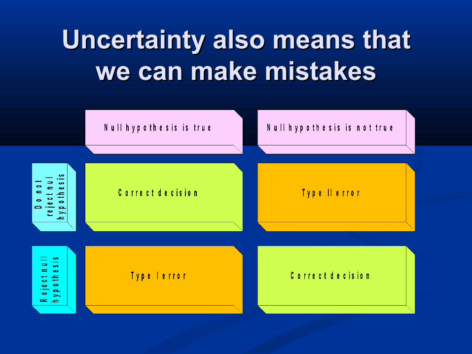
Uncertainty also means thatUncertainty also means thatwe can make mistakeswe can make mistakes

Type I and Type II errorsType I and Type II errors

Ideally, both Type I and Type II errors Ideally, both Type I and Type II errors would be smallwould be small

In practice, the probability of a Type I In practice, the probability of a Type I error is the significance level error is the significance level

As this decreases, the probability of As this decreases, the probability of accepting a false null hypothesis accepting a false null hypothesis increasesincreases

We have to balance the two types of We have to balance the two types of error error

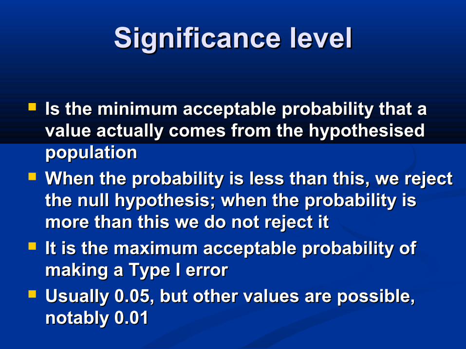
Significance levelSignificance level

Is the minimum acceptable probability that a Is the minimum acceptable probability that a value actually comes from the hypothesised value actually comes from the hypothesised populationpopulation

When the probability is less than this, we reject When the probability is less than this, we reject the null hypothesis; when the probability is the null hypothesis; when the probability is more than this we do not reject itmore than this we do not reject it

It is the maximum acceptable probability of It is the maximum acceptable probability of making a Type I errormaking a Type I error

Usually 0.05, but other values are possible, Usually 0.05, but other values are possible, notably 0.01notably 0.01

1 - 38

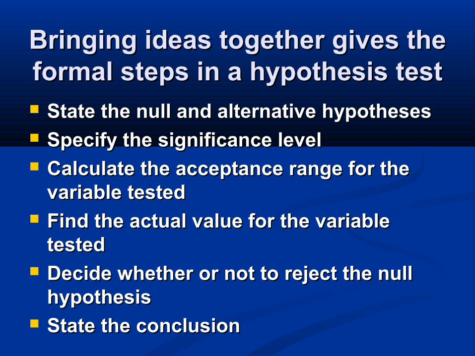
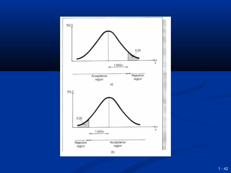
Bringing ideas together gives the Bringing ideas together gives the formal steps in a hypothesis testformal steps in a hypothesis test State the null and alternative hypothesesState the null and alternative hypotheses Specify the significance levelSpecify the significance level Calculate the acceptance range for the Calculate the acceptance range for the

variable testedvariable tested Find the actual value for the variable Find the actual value for the variable

testedtested Decide whether or not to reject the null Decide whether or not to reject the null

hypothesis hypothesis State the conclusion State the conclusion

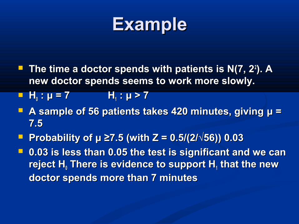
ExampleExample

The time a doctor spends with patients is N(7, 2The time a doctor spends with patients is N(7, 2 22). A ). A new doctor spends seems to work more slowly.new doctor spends seems to work more slowly.

HH00 : : μμ = 7 = 7 HH11 : : μμ > 7 > 7

A sample of 56 patients takes 420 minutes, giving A sample of 56 patients takes 420 minutes, giving μμ = = 7.57.5

Probability of Probability of μμ ≥7.5 (with Z = 0.5/(2/√56)) 0.03 ≥7.5 (with Z = 0.5/(2/√56)) 0.03 0.03 is less than 0.05 the test is significant and we can 0.03 is less than 0.05 the test is significant and we can

reject Hreject H00 There is evidence to support H There is evidence to support H11 that the new that the new

doctor spends more than 7 minutes doctor spends more than 7 minutes

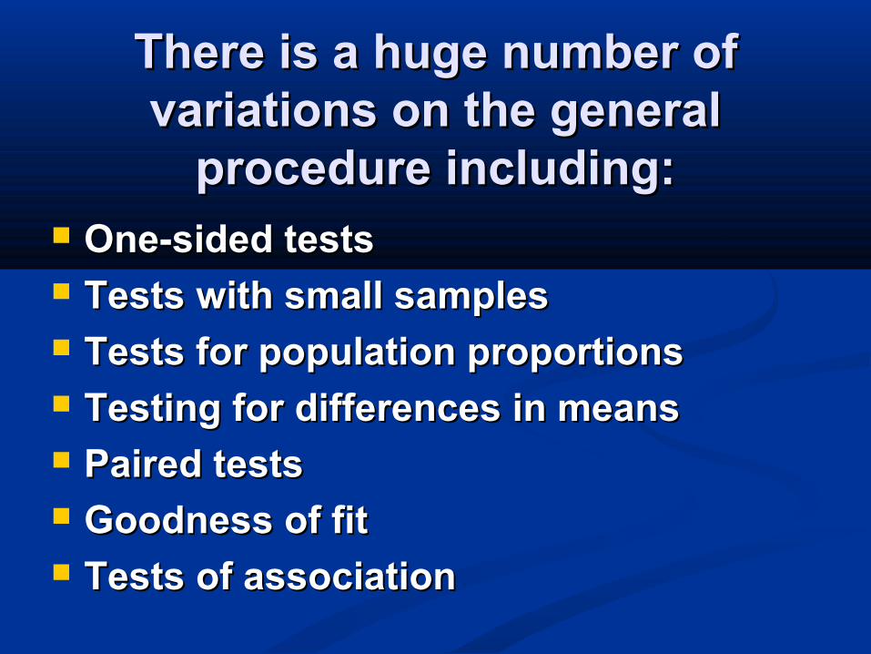
There is a huge number of There is a huge number of variations on the general variations on the general

procedure including:procedure including: One-sided testsOne-sided tests Tests with small samplesTests with small samples Tests for population proportionsTests for population proportions Testing for differences in meansTesting for differences in means Paired testsPaired tests Goodness of fitGoodness of fit Tests of associationTests of association

1 - 42

1 - 43

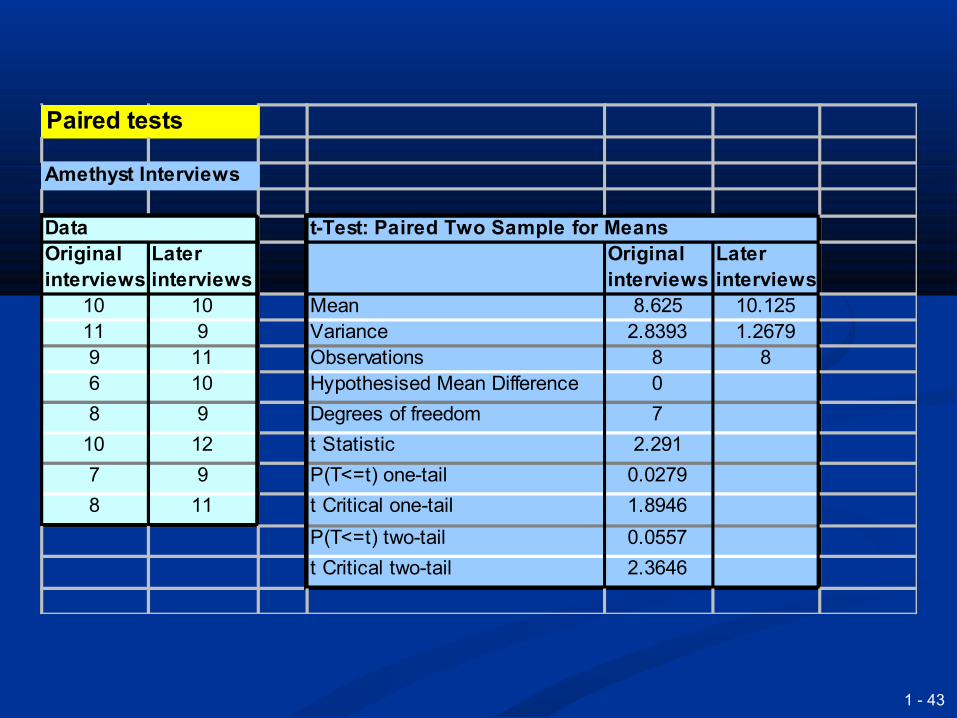
DataOriginal interviews

Later interviews

Original interviews

Later interviews

10 10 Mean 8.625 10.12511 9 Variance 2.8393 1.26799 11 Observations 8 86 10 Hypothesised Mean Difference 0

8 9 Degrees of freedom 7

10 12 t Statistic 2.291

7 9 P(T<=t) one-tail 0.0279

8 11 t Critical one-tail 1.8946

P(T<=t) two-tail 0.0557

t Critical two-tail 2.3646

Paired tests

Amethyst Interviews

t-Test: Paired Two Sample for Means

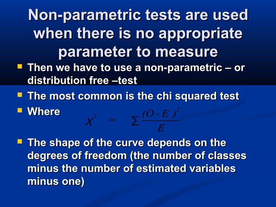
Non-parametric tests are used Non-parametric tests are used when there is no appropriate when there is no appropriate

parameter to measureparameter to measure Then we have to use a non-parametric – or Then we have to use a non-parametric – or

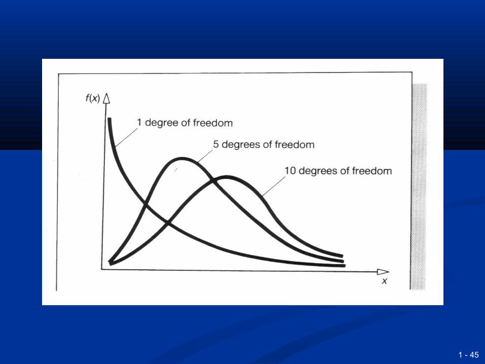
distribution free –testdistribution free –test The most common is the chi squared The most common is the chi squared testtest WhereWhere

The shape of the curve depends on the The shape of the curve depends on the degrees of freedom (the number of classes degrees of freedom (the number of classes minus the number of estimated variables minus the number of estimated variables minus one) minus one)

E

)E(O =

22 -∑χ

1 - 45

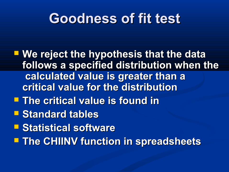
Goodness of fit testGoodness of fit test

We reject the hypothesis that the data We reject the hypothesis that the data follows a specified distribution when the follows a specified distribution when the calculated value is greater than a calculated value is greater than a critical value for the distributioncritical value for the distribution

The critical value is found inThe critical value is found in Standard tablesStandard tables Statistical softwareStatistical software The CHIINV function in spreadsheetsThe CHIINV function in spreadsheets

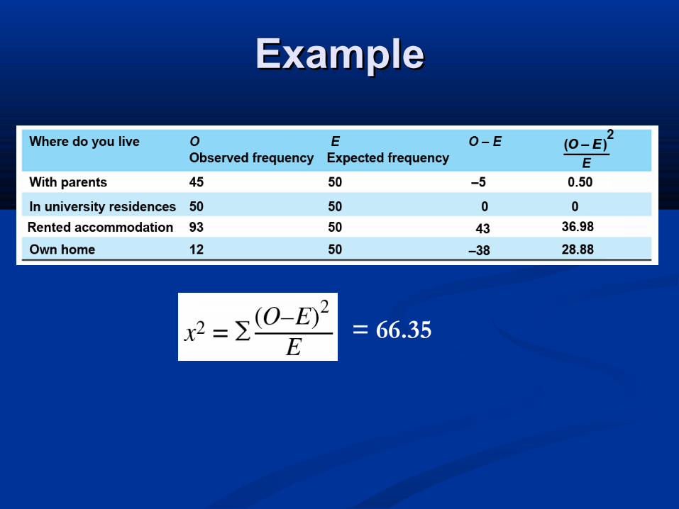
ExampleExample

= 66.35

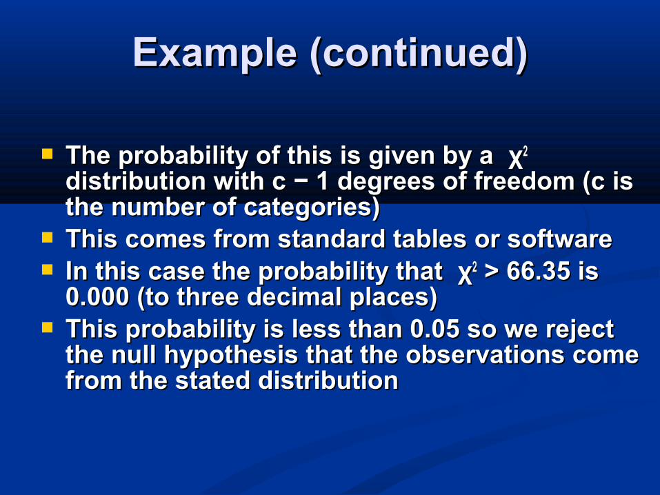
The probability of this is given by a The probability of this is given by a χχ22 distribution with c distribution with c −− 1 degrees of freedom (c is 1 degrees of freedom (c is the number of categories)the number of categories)

This comes from standard tables or softwareThis comes from standard tables or software In this case the probability that In this case the probability that χχ22 > 66.35 is > 66.35 is

0.000 (to three decimal places)0.000 (to three decimal places) This probability is less than 0.05 so we reject This probability is less than 0.05 so we reject

the null hypothesis that the observations come the null hypothesis that the observations come from the stated distributionfrom the stated distribution

Example (continued)Example (continued)

There are five categories so we need the χ2 distribution with5 – 1 = 4 degrees of freedom and then P (2 > 11.389) = 0.0225. This is less than 0.05 so we conclude that there is evidence that the probability distribution differs from the hypothesised one.

Example (continued)Example (continued)

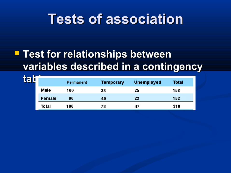
Tests of associationTests of association

Test for relationships between Test for relationships between variables described in a contingency variables described in a contingency table table

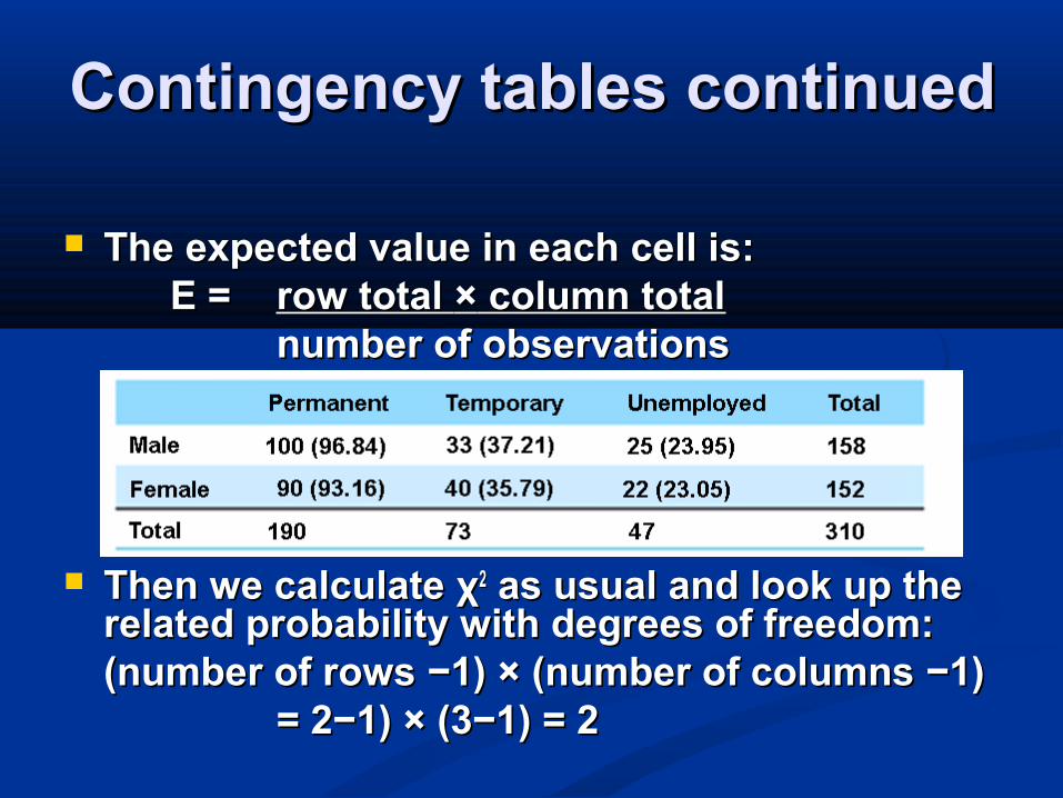
Contingency tables continuedContingency tables continued

The expected value in each cell is:The expected value in each cell is:E = E = row total row total ×× column total column total

number of observationsnumber of observations

Then we calculate Then we calculate χχ22 as usual and look up the as usual and look up the related probability with degrees of freedom:related probability with degrees of freedom:(number of rows (number of rows −−1) 1) ×× (number of columns (number of columns −−1) 1)

= 2= 2−−1) 1) ×× (3 (3−−1) = 21) = 2

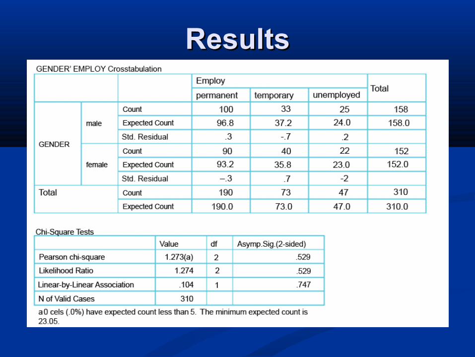
ResultsResults

REGRESSIONREGRESSION

1 - 53

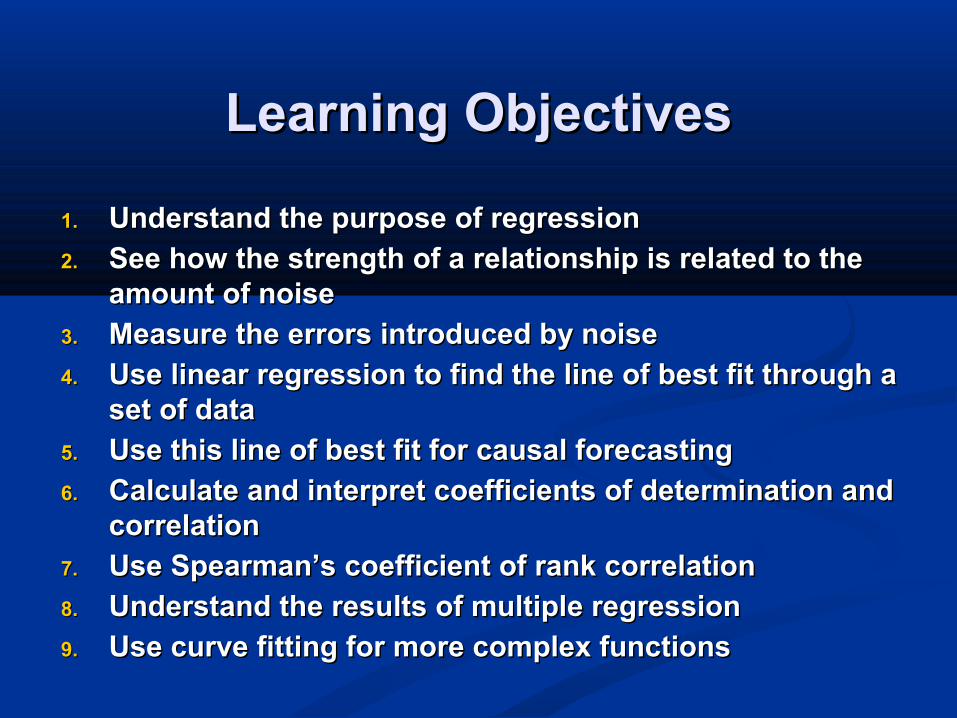
Learning ObjectivesLearning Objectives

1.1. Understand the purpose of regressionUnderstand the purpose of regression

2.2. See how the strength of a relationship is related to the See how the strength of a relationship is related to the amount of noiseamount of noise

3.3. Measure the errors introduced by noiseMeasure the errors introduced by noise

4.4. Use linear regression to find the line of best fit through a Use linear regression to find the line of best fit through a set of dataset of data

5.5. Use this line of best fit for causal forecastingUse this line of best fit for causal forecasting

6.6. Calculate and interpret coefficients of determination and Calculate and interpret coefficients of determination and correlationcorrelation

7.7. Use Spearman’s coefficient of rank correlationUse Spearman’s coefficient of rank correlation

8.8. Understand the results of multiple regressionUnderstand the results of multiple regression

9.9. Use curve fitting for more complex functionsUse curve fitting for more complex functions

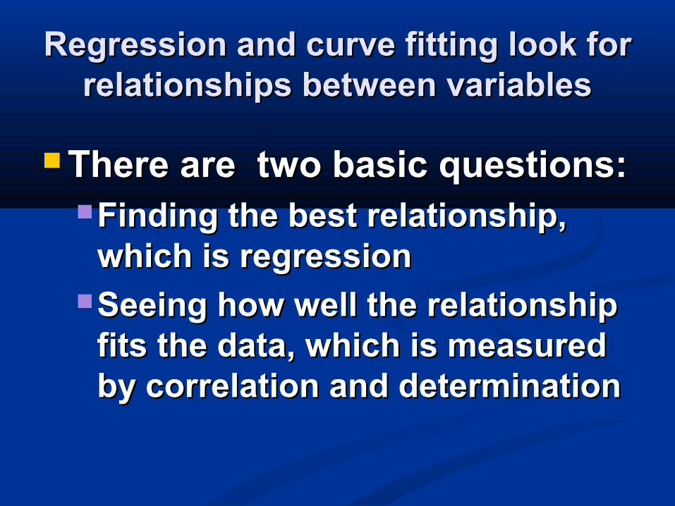
Regression and curve fitting look for Regression and curve fitting look for relationships between variablesrelationships between variables

There are two basic questions:There are two basic questions: Finding the best relationship, Finding the best relationship,

which is regressionwhich is regression Seeing how well the relationship Seeing how well the relationship

fits the data, which is measured fits the data, which is measured by correlation and determination by correlation and determination

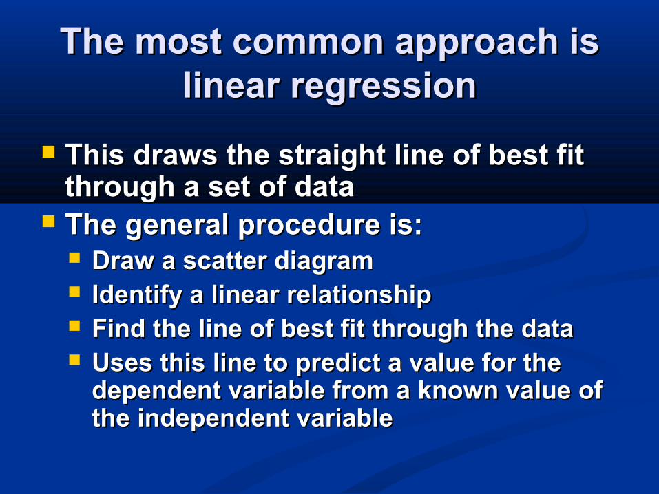
The most common approach is The most common approach is linear regressionlinear regression

This draws the straight line of best fit This draws the straight line of best fit through a set of datathrough a set of data

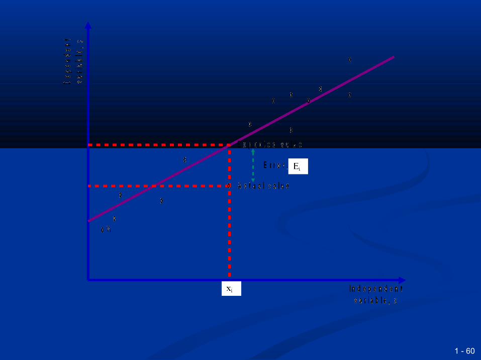
The general procedure is: The general procedure is: Draw a scatter diagramDraw a scatter diagram Identify a linear relationshipIdentify a linear relationship Find the line of best fit through the dataFind the line of best fit through the data Uses this line to predict a value for the Uses this line to predict a value for the

dependent variable from a known value of dependent variable from a known value of the independent variablethe independent variable

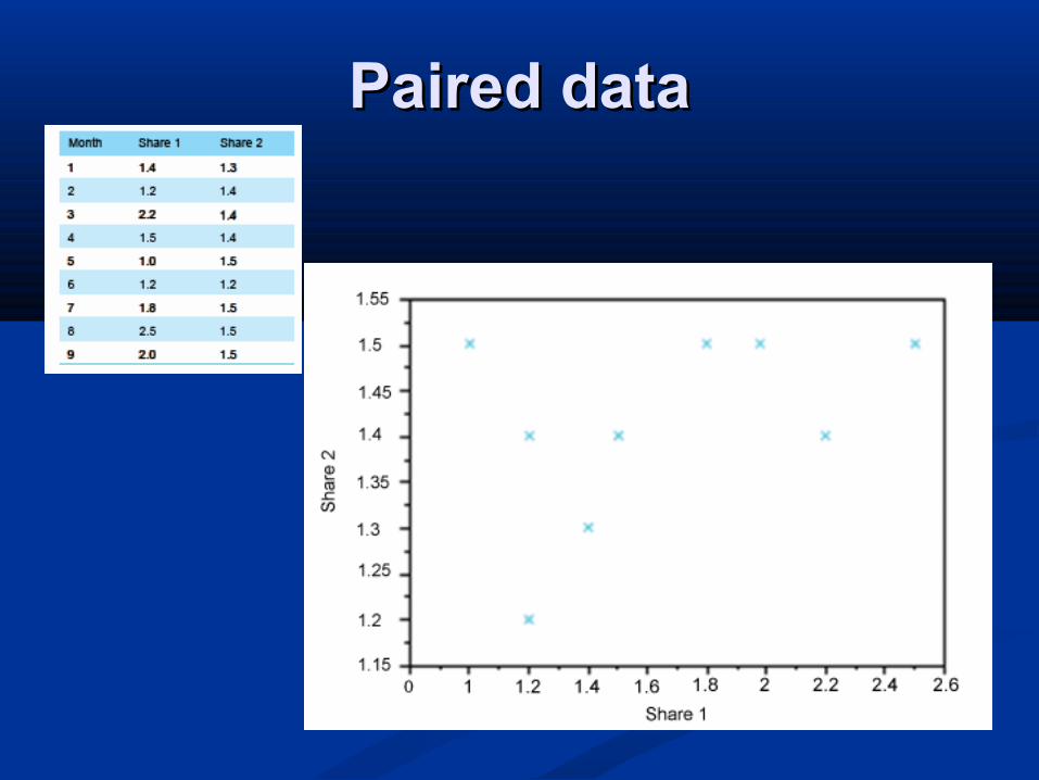
Paired dataPaired data

1 - 58

0

5

10

15

20

25

30

35

40

45

0 2 4 6 8 10 12 14 16 18

Temperature

Ele

ctr

icit

y c

on

su

pm

tio

n

Underlying trend

Some noise

More noise

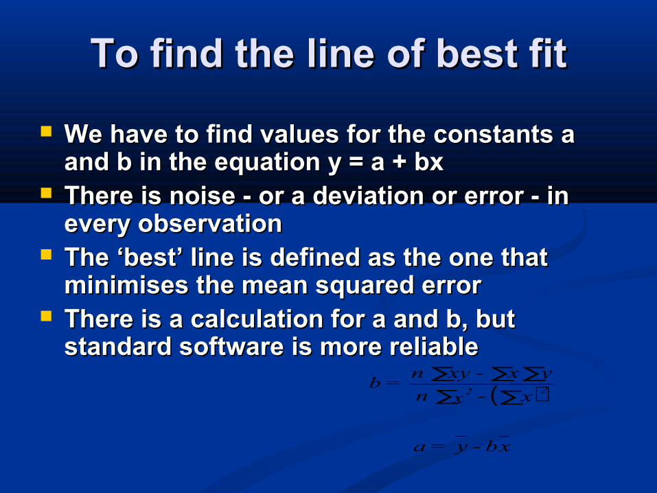
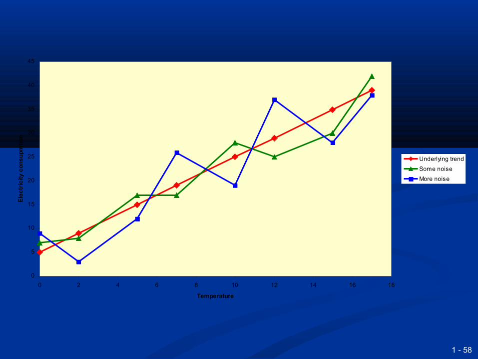
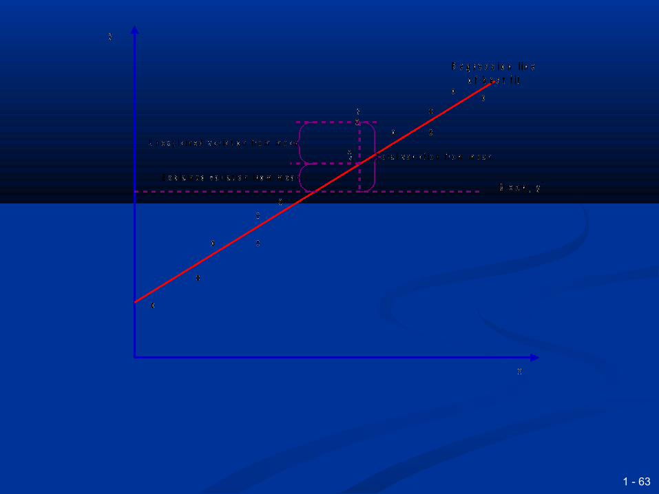
To find the line of best fitTo find the line of best fit

We have to find values for the constants a We have to find values for the constants a and b in the equation y = a + bx and b in the equation y = a + bx

There is noise - or a deviation or error - in There is noise - or a deviation or error - in every observationevery observation

The ‘best’ line is defined as the one that The ‘best’ line is defined as the one that minimises the mean squared errorminimises the mean squared error

There is a calculation for a and b, but There is a calculation for a and b, but standard software is more reliablestandard software is more reliable

( )

xb - y=a

x - xn

yx - xyn=b

22 ∑∑∑∑∑

1 - 60

1 - 61

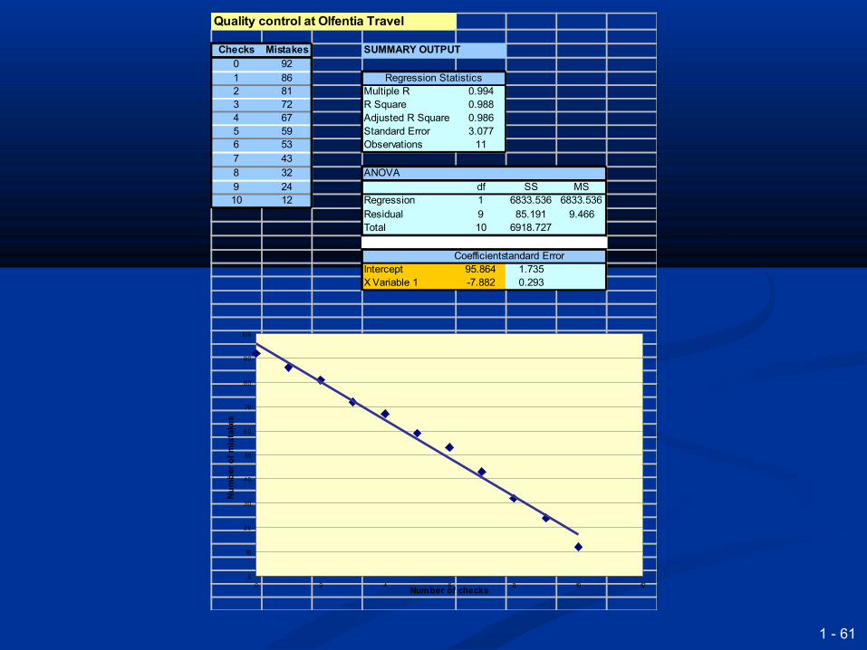
Quality control at Olfentia Travel

Checks Mistakes SUMMARY OUTPUT0 921 86 Regression Statistics2 81 Multiple R 0.9943 72 R Square 0.9884 67 Adjusted R Square 0.9865 59 Standard Error 3.0776 53 Observations 117 438 32 ANOVA9 24 df SS MS10 12 Regression 1 6833.536 6833.536

Residual 9 85.191 9.466Total 10 6918.727

CoefficientsStandard ErrorIntercept 95.864 1.735X Variable 1 -7.882 0.293

0

10

20

30

40

50

60

70

80

90

100

0 2 4 6 8 10 12Number of checks

Nu

mb

er o

f m

ista

kes

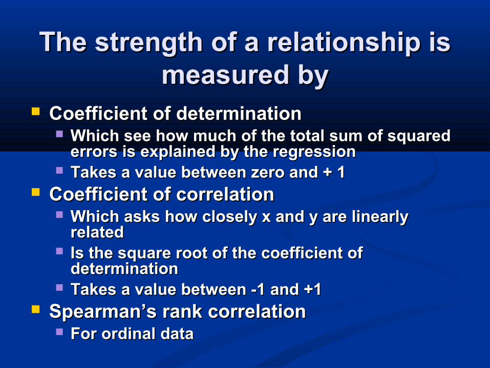
The strength of a relationship is The strength of a relationship is measured bymeasured by

Coefficient of determination Coefficient of determination Which see how much of the total sum of squared Which see how much of the total sum of squared

errors is explained by the regressionerrors is explained by the regression Takes a value between zero and + 1Takes a value between zero and + 1

Coefficient of correlation Coefficient of correlation Which asks how closely x and y are linearly Which asks how closely x and y are linearly

relatedrelated Is the square root of the coefficient of Is the square root of the coefficient of

determinationdetermination Takes a value between -1 and +1Takes a value between -1 and +1

Spearman’s rank correlationSpearman’s rank correlation For ordinal dataFor ordinal data

1 - 63

1 - 64

yy

x x

y y

x x

y

xx

y

o o

o

o

o

o

o

o

o

o

o

o

o

o

o

o

oo

o

o

o

o

o

o

o

o

o

o

o

o

o

o

o

o

o

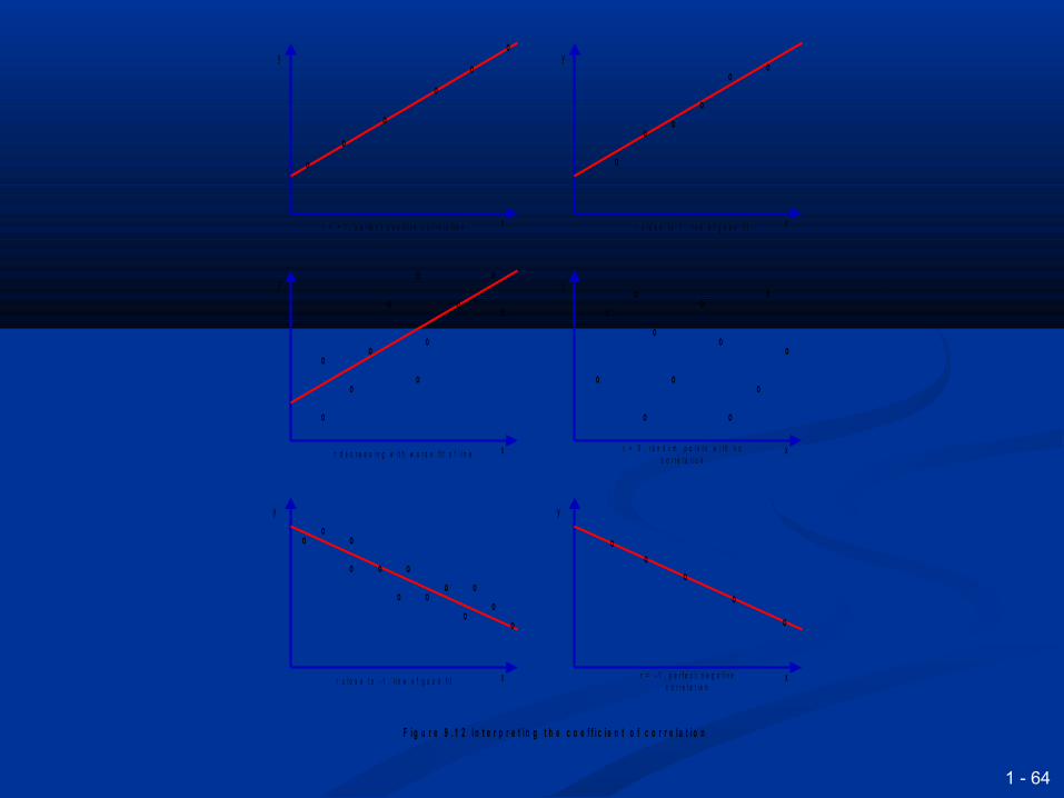
r = + 1 , p e r f e c t p o s i t i v e c o r r e l a t i o n r c l o s e t o 1 , l i n e o f g o o d f i t

r = 0 , r a n d o m p o i n t s w i t h n o c o r r e l a t i o n

r d e c r e a s i n g w i t h w o r s e f i t o f l i n e

r c l o s e t o - 1 , l i n e o f g o o d f i tr = - 1 , p e r f e c t n e g a t i v e

c o r r e l a t i o n

o

o

o

o

o

o

o

o

o

o

o

o o

o

o

o

o

o

F i g u r e 9 . 1 2 I n t e r p r e t i n g t h e c o e f f i c i e n t o f c o r r e l a t i o n

1 - 65

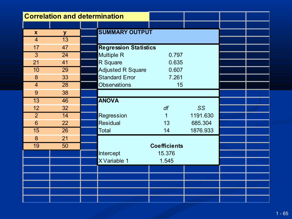
Correlation and determination

x y SUMMARY OUTPUT4 13

17 47 Regression Statistics3 24 Multiple R 0.797

21 41 R Square 0.63510 29 Adjusted R Square 0.6078 33 Standard Error 7.2614 28 Observations 159 38

13 46 ANOVA12 32 df SS2 14 Regression 1 1191.6306 22 Residual 13 685.304

15 26 Total 14 1876.9338 21

19 50 CoefficientsIntercept 15.376X Variable 1 1.545

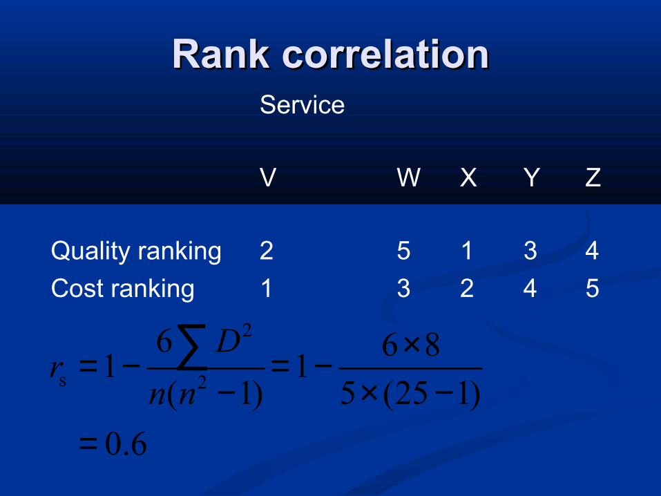
Rank correlationRank correlation

2

s 2

6 6 81   1

( 1) 5 (25 1)

  0.6

Dr

n n

×= − = −− × −

=

∑

Service

V W X Y Z

Quality ranking 2 5 1 3 4

Cost ranking 1 3 2 4 5

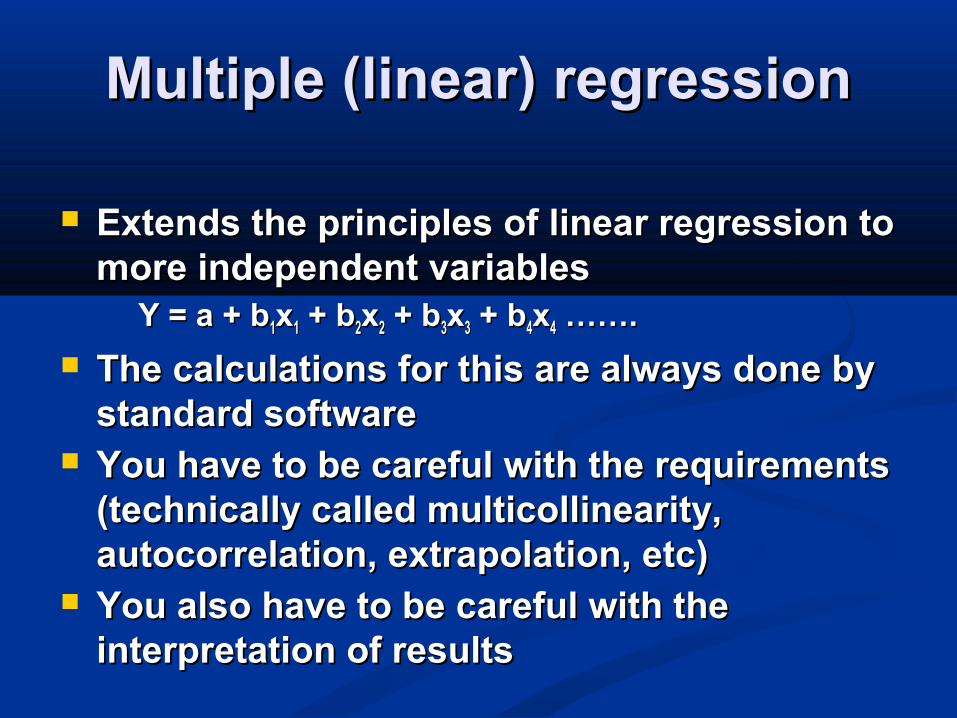
Multiple (linear) regressionMultiple (linear) regression

Extends the principles of linear regression to Extends the principles of linear regression to more independent variablesmore independent variables

Y = a + bY = a + b11xx11 + b + b22xx22 + b + b33xx33 + b + b44xx44 ……. …….

The calculations for this are always done by The calculations for this are always done by standard softwarestandard software

You have to be careful with the requirements You have to be careful with the requirements (technically called multicollinearity, (technically called multicollinearity, autocorrelation, extrapolation, etc)autocorrelation, extrapolation, etc)

You also have to be careful with the You also have to be careful with the interpretation of results interpretation of results

1 - 68

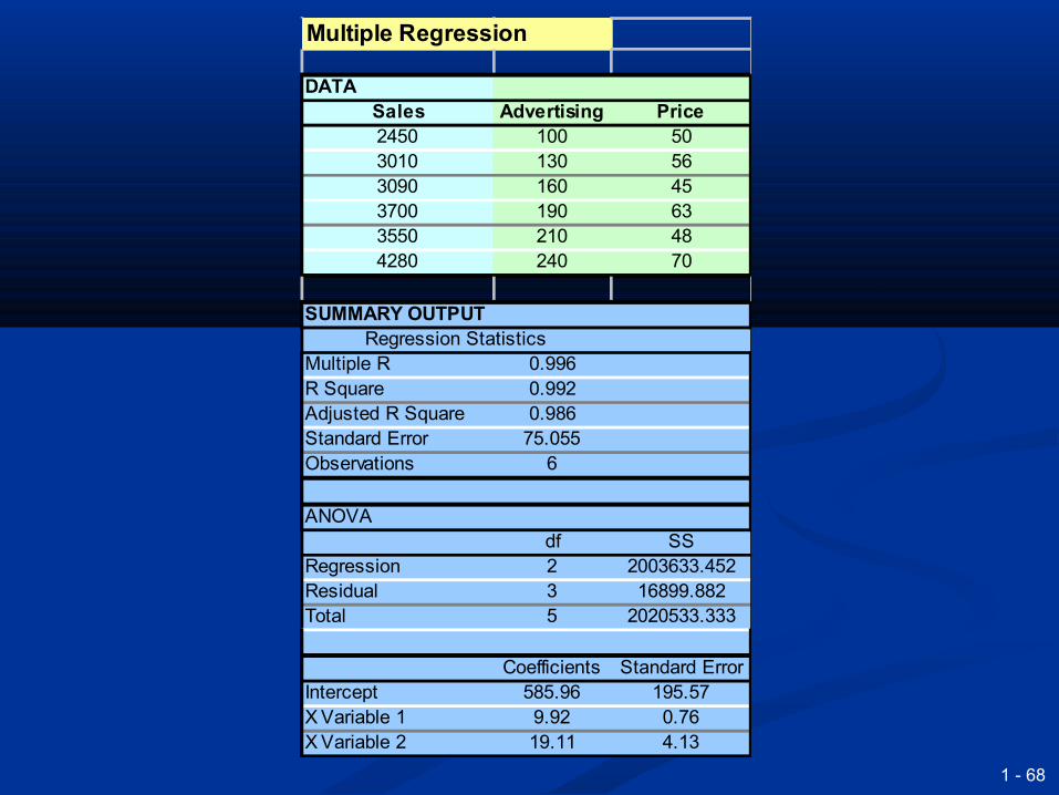
Multiple Regression

DATASales Advertising Price2450 100 503010 130 563090 160 453700 190 633550 210 484280 240 70

SUMMARY OUTPUTRegression Statistics

Multiple R 0.996R Square 0.992Adjusted R Square 0.986Standard Error 75.055Observations 6

ANOVAdf SS

Regression 2 2003633.452Residual 3 16899.882Total 5 2020533.333

Coefficients Standard ErrorIntercept 585.96 195.57X Variable 1 9.92 0.76X Variable 2 19.11 4.13

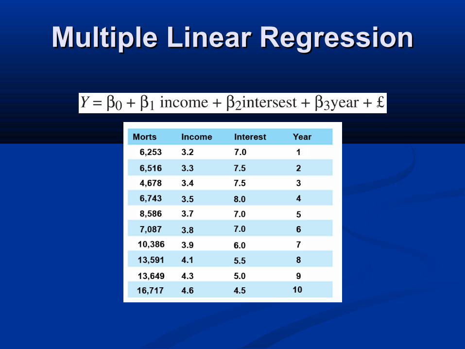
Multiple Linear RegressionMultiple Linear Regression

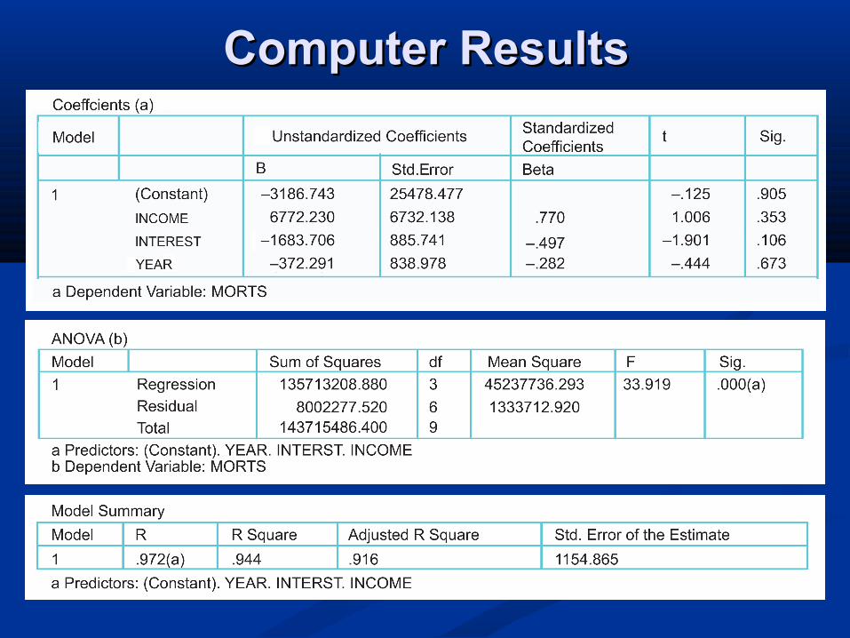
Computer ResultsComputer Results

1 - 71

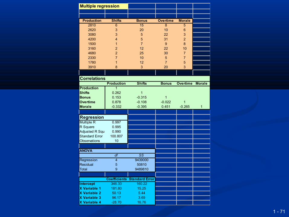
Multiple regression

Production Shifts Bonus Overtime Morale2810 6 15 8 52620 3 20 10 63080 3 5 22 34200 4 5 31 21500 1 7 9 83160 2 12 22 104680 2 25 30 72330 7 10 5 71780 1 12 7 53910 8 3 20 3

CorrelationsProduction Shifts Bonus Overtime Morale

Production 1Shifts 0.262 1Bonus 0.153 -0.315 1Overtime 0.878 -0.108 -0.022 1Morale -0.332 -0.395 0.451 -0.265 1

RegressionMultiple R 0.997R Square 0.995Adjusted R Square 0.990Standard Error 100.807Observations 10

ANOVAdf SS

Regression 4 9439000Residual 5 50810Total 9 9489810

Coefficients Standard ErrorIntercept 346.33 160.22X Variable 1 181.80 15.25X Variable 2 50.13 5.44X Variable 3 96.17 3.69X Variable 4 -28.70 16.76

Curve fittingCurve fitting

Is a more general term than regressionIs a more general term than regression It refers to the process of fitting It refers to the process of fitting

different types of curve through sets of different types of curve through sets of datadata

Typically this involves:Typically this involves: Exponential curvesExponential curves Growth curvesGrowth curves PolynomialsPolynomials

1 - 73

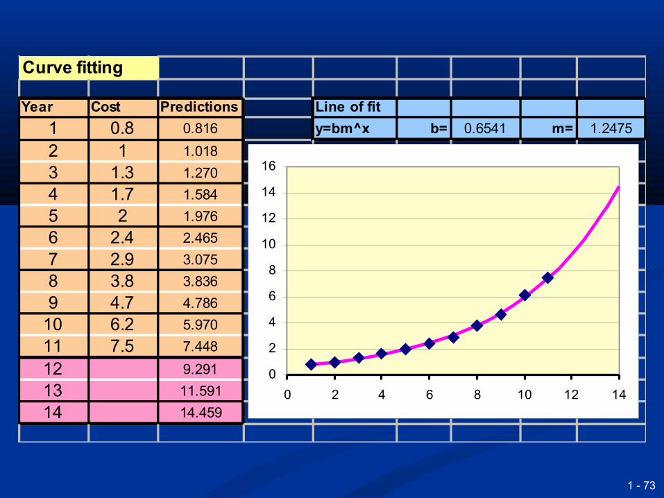
Curve fitting

Year Cost Predictions Line of fit

1 0.8 0.816 y=bm^x b= 0.6541 m= 1.2475

2 1 1.018

3 1.3 1.270

4 1.7 1.584

5 2 1.976

6 2.4 2.465

7 2.9 3.075

8 3.8 3.836

9 4.7 4.786

10 6.2 5.970

11 7.5 7.448

12 9.291

13 11.591

14 14.459

0

2

4

6

8

10

12

14

16

0 2 4 6 8 10 12 14

Further ReadingFurther Reading

Waters, Donald (2011) Quantitative Waters, Donald (2011) Quantitative Methods for Business, Prentice Hall, 5Methods for Business, Prentice Hall, 5 thth EditionEdition

Evans, J.R (2013), Business Evans, J.R (2013), Business Analytics, Analytics, 1st Edition1st Edition Pearson Pearson

Render, B., Stair Jr.,R.M. & Hanna, M.E. (2013) Quantitative Analysis for Management, Pearson, 11th Edition

QUESTIONS?QUESTIONS?