Revisiting Unit Root, Autocorrelation and Multicollinearity

Gaetan Lion

July 2015

revised and expanded vs. earlier version

1

Unit Root

2

Unit Root basics

A Unit Root is a problem that occurs when the best estimate of Y is Y t-1, and that coefficient* is very close to 1 or higher (or lower).

This denotes a Y variable that is non-stationary and does not mean-revert (or not mean-revert fast enough).

The average and the variance of Y are unstable.

In such a situation, you will get “spurious” regression results with high R^2, high t-stat, and often Durbin Watson < 1 (high autocorrelation) but no economic meaning.

If you detrend Y, the resulting Goodness-of-fit of detrended estimates and performance in Hold Out could be really poor.

3

*Y = b Y t-1

How to test for Unit Root?

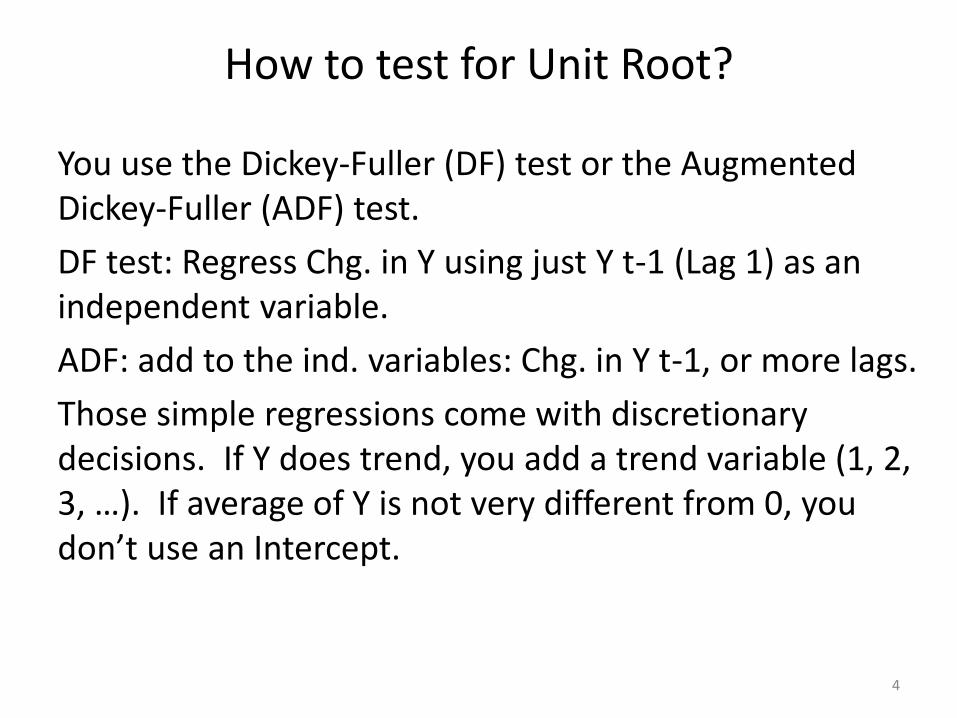
You use the Dickey-Fuller (DF) test or the Augmented Dickey-Fuller (ADF) test.

DF test: Regress Chg. in Y using just Y t-1 (Lag 1) as an independent variable.

ADF: add to the ind. variables: Chg. in Y t-1, or more lags.

Those simple regressions come with discretionary decisions. If Y does trend, you add a trend variable (1, 2, 3, …). If average of Y is not very different from 0, you don’t use an Intercept.

4

How to structure a Dependent Variable, Real GDP Growth?

5

Unit root test (nonstationary): Unit root test (nonstationary): Unit root test (nonstationary):

tau Stat Critic. val. Type tau Stat Critic. val. Type tau Stat Critic. val. Type

Dickey-Fuller -1.12 -3.15 with Constant, with Trend Dickey-Fuller -0.83 -3.15 with Constant, with Trend Dickey-Fuller -6.79 -2.58 with Constant, no Trend

Augmented DF -4.74 -2.58 with Constant, no Trend

$-

$2,000

$4,000

$6,000

$8,000

$10,000

$12,000

$14,000

$16,000

$18,000

19

82q

1

19

83q

3

19

85q

1

19

86q

3

19

88q

1

19

89q

3

19

91q

1

19

92q

3

19

94q

1

19

95q

3

19

97q

1

19

98q

3

20

00q

1

20

01q

3

20

03q

1

20

04q

3

20

06q

1

20

07q

3

20

09q

1

20

10q

3

20

12q

1

20

13q

3

Real GDP in 2009 $mm

8.20

8.40

8.60

8.80

9.00

9.20

9.40

9.60

9.80

19

82q

1

19

83q

3

19

85q

1

19

86q

3

19

88q

1

19

89q

3

19

91q

1

19

92q

3

19

94q

1

19

95q

3

19

97q

1

19

98q

3

20

00q

1

20

01q

3

20

03q

1

20

04q

3

20

06q

1

20

07q

3

20

09q

1

20

10q

3

20

12q

1

20

13q

3

LN(Real GDP in 2009 $)

-10.0%

-8.0%

-6.0%

-4.0%

-2.0%

0.0%

2.0%

4.0%

6.0%

8.0%

10.0%

12.0%

19

82q

1

19

83q

3

19

85q

1

19

86q

3

19

88q

1

19

89q

3

19

91q

1

19

92q

3

19

94q

1

19

95q

3

19

97q

1

19

98q

3

20

00q

1

20

01q

3

20

03q

1

20

04q

3

20

06q

1

20

07q

3

20

09q

1

20

10q

3

20

12q

1

20

13q

3

Real GDP Growth quarterly % chg. annualized

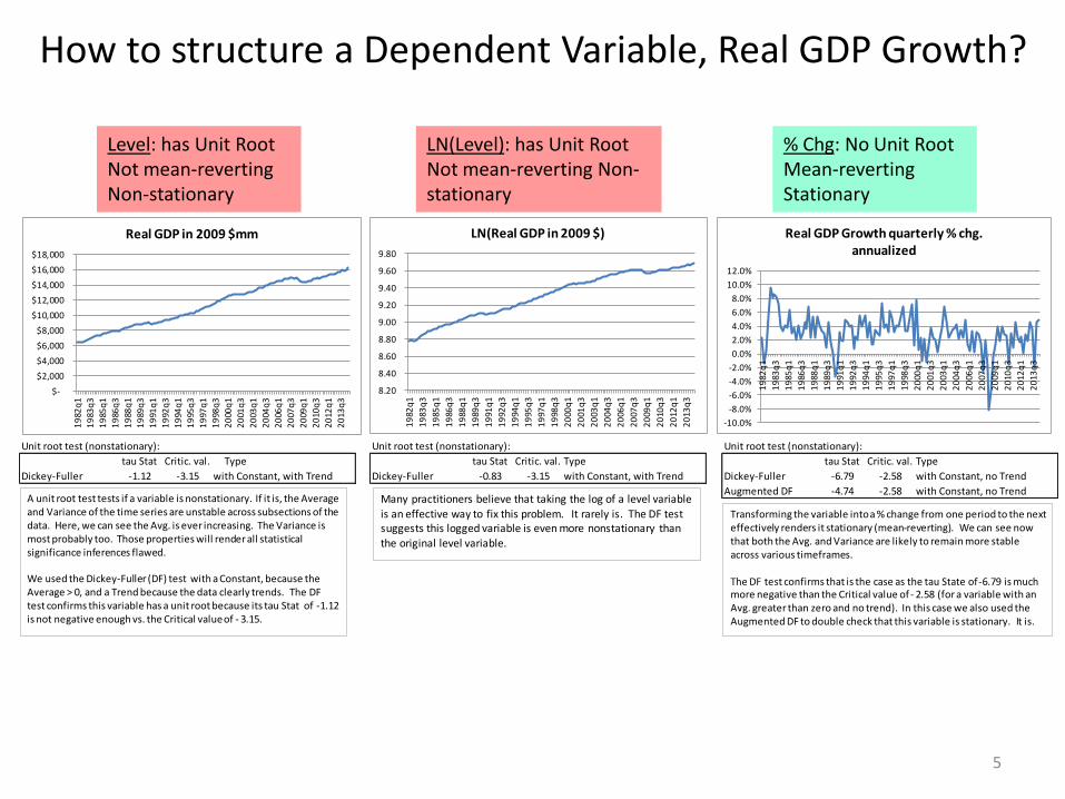
A unit root test tests if a variable is nonstationary. If it is, the Average and Variance of the time series are unstable across subsections of the data. Here, we can see the Avg. is ever increasing. The Variance is most probably too. Those properties will render all statistical significance inferences flawed.

We used the Dickey-Fuller (DF) test with a Constant, because the Average > 0, and a Trend because the data clearly trends. The DF test confirms this variable has a unit root because its tau Stat of -1.12 is not negative enough vs. the Critical value of - 3.15.

Many practitioners believe that taking the log of a level variable is an effective way to fix this problem. It rarely is. The DF test suggests this logged variable is even more nonstationary than the original level variable.

Transforming the variable intoa % change from one period to the next effectively renders it stationary (mean-reverting). We can see now that both the Avg. and Variance are likely to remain more stable across various timeframes.

The DF test confirms that is the case as the tau State of -6.79 is much more negative than the Critical value of - 2.58 (for a variable with an Avg. greater than zero and no trend). In this case we also used the Augmented DF to double check that this variable is stationary. It is.

Level: has Unit RootNot mean-reverting Non-stationary

LN(Level): has Unit RootNot mean-reverting Non-stationary

% Chg: No Unit Root Mean-reverting Stationary

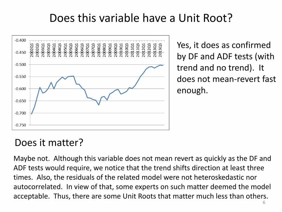
Does this variable have a Unit Root?

6

Yes, it does as confirmed by DF and ADF tests (with trend and no trend). It does not mean-revert fast enough.

Does it matter?

Maybe not. Although this variable does not mean revert as quickly as the DF and ADF tests would require, we notice that the trend shifts direction at least three times. Also, the residuals of the related model were not heteroskedastic nor autocorrelated. In view of that, some experts on such matter deemed the model acceptable. Thus, there are some Unit Roots that matter much less than others.

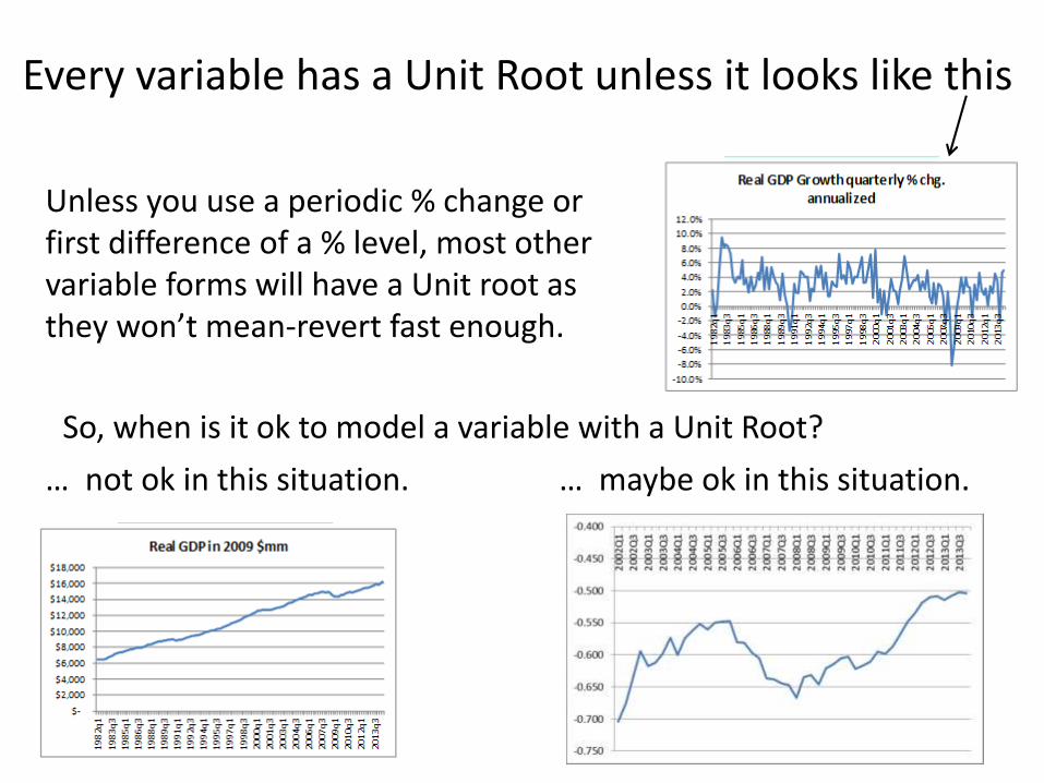
Every variable has a Unit Root unless it looks like this

7

Unless you use a periodic % change or first difference of a % level, most other variable forms will have a Unit root as they won’t mean-revert fast enough.

So, when is it ok to model a variable with a Unit Root?

… maybe ok in this situation. … not ok in this situation.

When is a Unit Root acceptable?

8

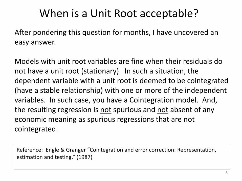
After pondering this question for months, I have uncovered an easy answer.

Models with unit root variables are fine when their residuals do not have a unit root (stationary). In such a situation, the dependent variable with a unit root is deemed to be cointegrated (have a stable relationship) with one or more of the independent variables. In such case, you have a Cointegration model. And, the resulting regression is not spurious and not absent of any economic meaning as spurious regressions that are not cointegrated.

Reference: Engle & Granger “Cointegration and error correction: Representation, estimation and testing.” (1987)

When to consider Cointegration Models

9

• When detrending the variable anymore appears to generate more noise regarding the relationship between variables;

• The variables with Unit Root are constrained. Thus, they do not grow forever. Examples include unemployment rate, interest rates, and all variables constrained between 0 and 1. Such variables often have a unit root because their time series is too short to capture their mean reverting property;

• The regression model’s residuals are associated with no more than a moderate autocorrelation. A DW score < 1.00 may be deemed too low;

• The residuals tests well for stationarity. That’s the definition of a Cointegration model.

Unit Root testing revisited

10

The DF and ADF tests are helpful in diagnosing a Unit Root. And, they are helpful in diagnosing the potential absence of Unit Root in the residuals. But, a more appropriate test for testing whether the residuals are stationary is Phillips-Ouliaris. In such a situation (residuals stationary), your model is a Cointegration Model. And, you have overcome the issues with Unit Root and “spurious” regressions.

The term “spurious” is quoted from Granger & Newbold “Spurious regressions in econometrics” (1974).

Autocorrelation

11

Autocorrelation Quiz

12

A model’s residuals have a Durbin Watson score of 1.83 (excellent score denoting no autocorrelation) and an actual autocorrelation very close to Zero at 0.08.

Are the above residuals indeed not autocorrelated?

The Question is the Answer, as they say…

Durbin Watson is outdated

13

You still have to calculate it because everyone still uses it including SAS, STATA, EViews, etc…

Why is it outdated:1) It is highly imprecise associated with a large range of

uncertainty (as defined in DW tables);2) It can’t handle a model with autoregressive variables (Y t-1,

etc…);3) It can’t measure autocorrelation for other lags (t-1, t-2, etc…).

DW is being replaced by the Ljung-Box (LB) and Breusch-Godfrey (BG) tests that can handle all three situations mentioned above.

A broader autocorrelation framework

14

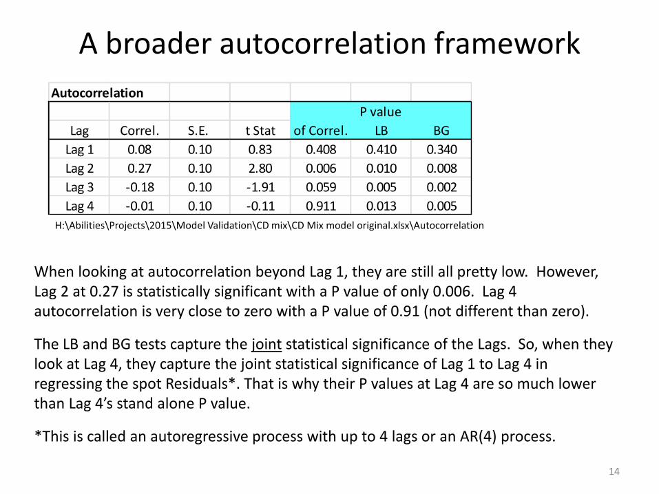
Autocorrelation

P value

Lag Correl. S.E. t Stat of Correl. LB BG

Lag 1 0.08 0.10 0.83 0.408 0.410 0.340

Lag 2 0.27 0.10 2.80 0.006 0.010 0.008

Lag 3 -0.18 0.10 -1.91 0.059 0.005 0.002

Lag 4 -0.01 0.10 -0.11 0.911 0.013 0.005

H:\Abilities\Projects\2015\Model Validation\CD mix\CD Mix model original.xlsx\Autocorrelation

When looking at autocorrelation beyond Lag 1, they are still all pretty low. However, Lag 2 at 0.27 is statistically significant with a P value of only 0.006. Lag 4 autocorrelation is very close to zero with a P value of 0.91 (not different than zero).

The LB and BG tests capture the joint statistical significance of the Lags. So, when they look at Lag 4, they capture the joint statistical significance of Lag 1 to Lag 4 in regressing the spot Residuals*. That is why their P values at Lag 4 are so much lower than Lag 4’s stand alone P value.

*This is called an autoregressive process with up to 4 lags or an AR(4) process.

Autocorrelation synthesis

15

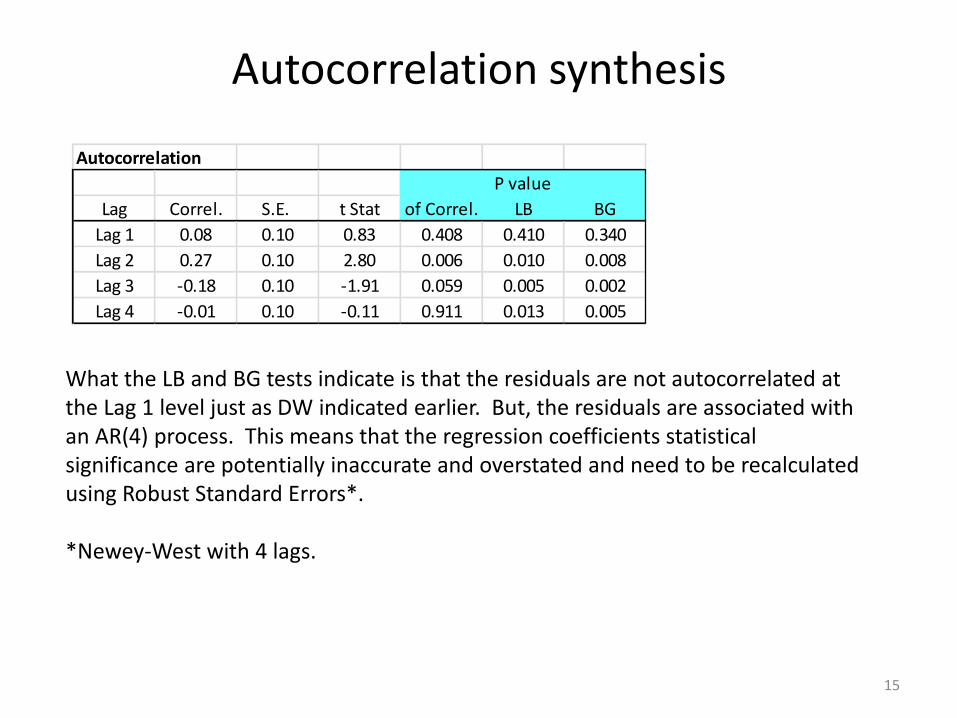
Autocorrelation

P value

Lag Correl. S.E. t Stat of Correl. LB BG

Lag 1 0.08 0.10 0.83 0.408 0.410 0.340

Lag 2 0.27 0.10 2.80 0.006 0.010 0.008

Lag 3 -0.18 0.10 -1.91 0.059 0.005 0.002

Lag 4 -0.01 0.10 -0.11 0.911 0.013 0.005

What the LB and BG tests indicate is that the residuals are not autocorrelated at the Lag 1 level just as DW indicated earlier. But, the residuals are associated with an AR(4) process. This means that the regression coefficients statistical significance are potentially inaccurate and overstated and need to be recalculated using Robust Standard Errors*.

*Newey-West with 4 lags.

Implication

16

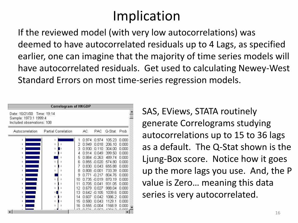
If the reviewed model (with very low autocorrelations) was deemed to have autocorrelated residuals up to 4 Lags, as specified earlier, one can imagine that the majority of time series models will have autocorrelated residuals. Get used to calculating Newey-West Standard Errors on most time-series regression models.

SAS, EViews, STATA routinely generate Correlograms studying autocorrelations up to 15 to 36 lags as a default. The Q-Stat shown is the Ljung-Box score. Notice how it goes up the more lags you use. And, the P value is Zero… meaning this data series is very autocorrelated.

Multicollinearity

17

Multicollinearity: The main issues

18

1) Regression coefficients will have much larger standard errors and lower statistical significance than otherwise;

2) As the R^2 of the regression model testing for multicollinearity approaches 1, 1 – R^2 approaches 0. At some point, this renders the inversion of the underlying matrix calculation between unstable to impossible as a quantity divided by 0 is undefined;

3) Potentially, large changes in regression coefficients when the multicollinear variable is removed.

The Basic Multicollinearity Framework

19

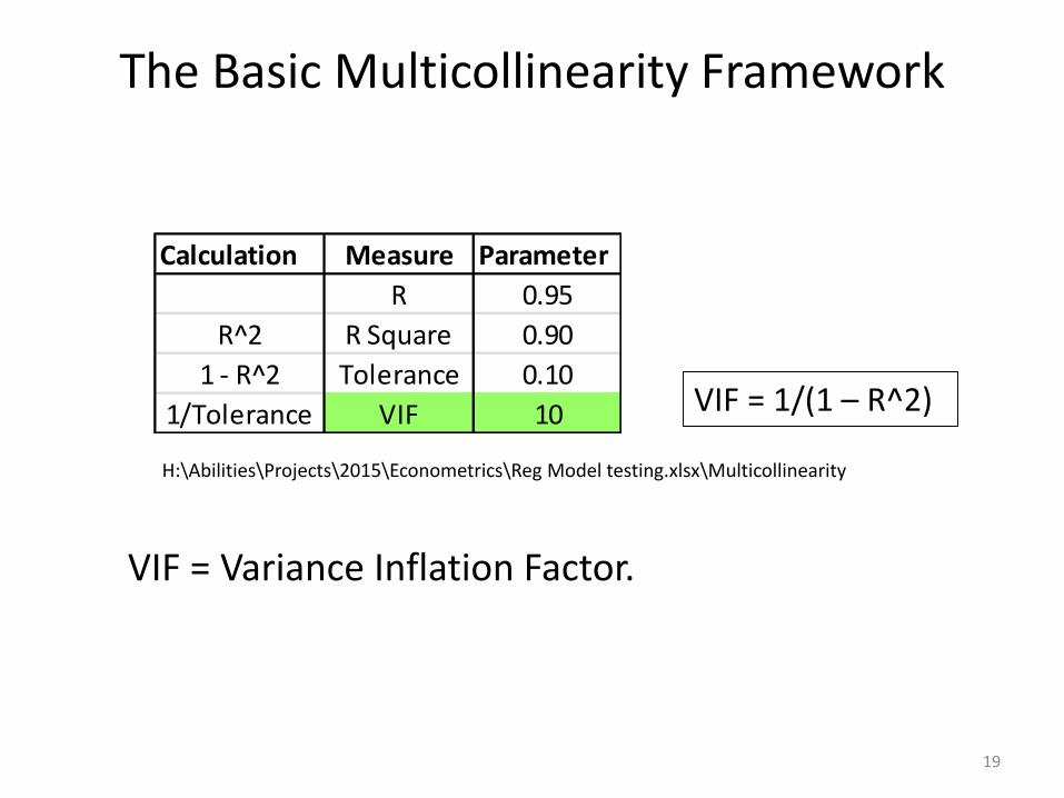
H:\Abilities\Projects\2015\Econometrics\Reg Model testing.xlsx\Multicollinearity

VIF = 1/(1 – R^2)

Calculation Measure Parameter

R 0.95

R^2 R Square 0.90

1 - R^2 Tolerance 0.10

1/Tolerance VIF 10

VIF = Variance Inflation Factor.

An Emerging New Standard: SQRT(VIF) = 2

20

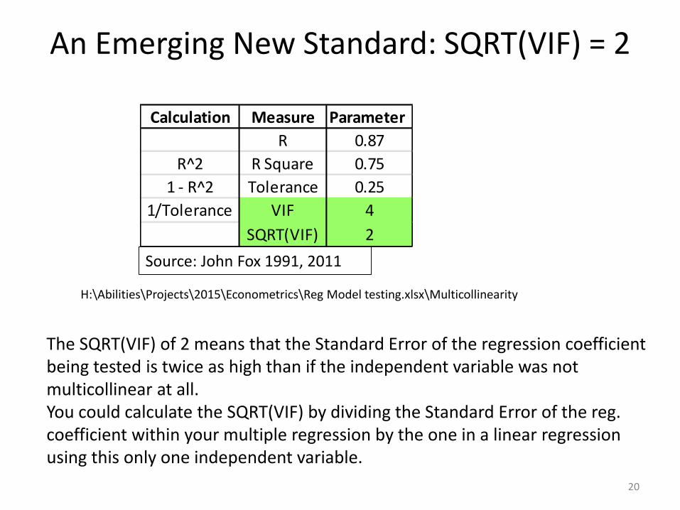
Calculation Measure Parameter

R 0.87

R^2 R Square 0.75

1 - R^2 Tolerance 0.25

1/Tolerance VIF 4

SQRT(VIF) 2

H:\Abilities\Projects\2015\Econometrics\Reg Model testing.xlsx\Multicollinearity

Source: John Fox 1991, 2011

The SQRT(VIF) of 2 means that the Standard Error of the regression coefficient being tested is twice as high than if the independent variable was not multicollinear at all.You could calculate the SQRT(VIF) by dividing the Standard Error of the reg. coefficient within your multiple regression by the one in a linear regression using this only one independent variable.

Does SQRT(VIF) = 2 matters?

21

It mainly matters if you are concerned about a TYPE II Error… rejecting an independent variable because of lack of statistical significance (accepting the null hypothesis that the regression coefficient is not different from zero). If tested variable is already stat. significant, SQRT(VIF) = 2 is not much of a concern.

Does VIF = 10 matters?

22

The answer is the same as for SQRT(VIF) = 2. VIF = 10 translates into boosting the Standard Error of the tested regression coefficient by 3.3 times. But, if the coefficient is already stat. significant this is not an issue.

How about the associated R^2 of 0.90 being close to destabilizing the calculations of inverting a matrix to resolve the original regression?

Any software algorithm can easily divide by 0.10. That’s not a problem. To be threatening, the R Square must be closer to something like 0.999… This in turn means that Correlation must be even closer to 1. Maybe VIF = 1,000,000 would be a problem… but not VIF = 10.

How about the change in regression coefficients when you remove a variable? It depends…

23

Let’s say you regress GNP growth as follows:

GNP = Const. + b1 S&P 500 + b2 Home price + b3 FF + b4 LIBOR

The regression coefficients for FF and LIBOR are both -0.10. You remove FF. LIBOR’s coefficient moves to -0.20 and the other two coefficients (Stock and Home prices) do not move much. Is that a problem? Probably not…

On the other hand, if they did move a lot that may be a problem. And, the weaker rate variable should probably be removed.

However, neither VIF = 10 nor SQRT(VIF) = 2 will give you any indication in what situation you are in. You’ll just have to try it out.