Embed Size (px)
Citation preview


II
خالصة الرسالة
محمد عبداهللا ايوب: اسم الطالب
تطوير واختبار نموذج لشبكة االعصاب االصطناعية للتنبؤ بضغط اآلبارالسفلى : عنوان الدراسة
.ذات السريان العمودى للموائع المتعددة االطوار
هندسة البترول: التخصص م 2004مارس : تأريخ الشهادة
صبية بنجاح لعمل نموذج للتنبؤ بضغط البئر السفلى فى آبارالنفط ذات ُأستخدمت تقنية الشبكات الع
التوجيه ( وقد تم تطوير النموذج الجديد بإستخدام خوارزمية للتعلم . السريان العمودى المتعددة االطوار
نقطة بيانات حقلية فى تطوير النموذج مأخوذة من عّدة حقول 206وقد ُأستخدمت ) . الخلفى لالخطاء
وتغطى البيانات المستخدمة فى تطوير النموذج معدل انتاج نفطى يتراوح . ة الشرق االوسط من منطق
% 44.8الى % 0.0 برميل فى اليوم، نسبة وجود الماء فى الموائع من 19618 الى 280ما بين
حتى لنفط ا الى لغاز ا نسبة برميل 675.5ووصلت لكل مكعب لمتاحة . قدم ا لبيانات ا تقسيم وعند
داء بالنسبة للنموذج أ على أ تم الحصول على 3:1:1بنسبة ) تدريب، الصالحية، واألختبار زمرة ال (
.المطور
أل رنة مقا دراسة ء إجرا تم لنماذج وقد وا لتجريبية ا لعالقات با رنته ومقا لمطور ا لنموذج ا ء ا د
لنماذج الميكانيستية االخرى باستخدام مقاييس احصائية وقد ُوجد ان اداء النموذج الُمطور يفوق ا
.االخرى والعالقات التجريبية بحصوله على أعلى معدل إرتباط وأقل أخطاء وإنحراف معيارى
وعند تطبيق النموذج الجديد، ينبغى األخذ بعين االعتبار نطاق البيانات الحقلية التى ُأستخدمت فى
.تطوير النموذج
درجة الماجستير فى العلومجامعة الملك فهد للبترول والمعادن
المملكة العربية السعودية-ظهرانال م 2004مارس

III
Thesis Abstract
Full Name of Student: Mohammed Abdalla Ayoub Title of Study: DEVELOPMENT AND TESTING OF AN ARTIFICIAL NEURAL
NETWORK MODEL FOR PREDICTING BOTTOMHOLE PRESSURE IN VERTICAL MULTIPHASE FLOW
Date of Degree: March 2004
A Neural Network technique has been used successfully for developing a model
for predicting bottomhole pressure in vertical multiphase flow in oil wells. The new
model has been developed using the most robust learning algorithm (back-propagation). A
total number of 206 data sets; collected from Middle East fields; has been used in
developing the model. The data used for developing the model covers an oil rate from 280
to 19618 BPD, water cut up to 44.8%, and gas oil ratios up to 675.5 SCF/STB. A ratio of
3:1:1 between training, validation, and testing sets yielded the best training/testing
performance. The best available empirical correlations and mechanistic models have been
tested against the data and the developed model.
Graphical and statistical tools have been utilized for the sake of comparing the
performance of the new model and other empirical correlations and mechanistic models.
Thorough verifications indicated that the new developed model outperforms all tested
empirical correlations and mechanistic models in terms of highest correlation coefficient,
lowest average absolute percent error, lowest standard deviation, lowest maximum error,
and lowest root mean square error. The new developed model results can only be used
within the range of used data; hence care should be taken if other data beyond this limit is
implemented.
MASTER OF SCIENCE DEGREE
KING FAHD UNIVERSITY OF PETROLEUM AND MINERALS
Dhahran-Saudi Arabia
Date: March 2004

IV
ACKNOWLEDGEMENT
All praise is due to Allah the most beneficent, the most compassionate, and peace is
upon his prophet Mohammed. I wish firstly to express my sincere gratitude and thanks to
KFUPM for providing me full financial support during the entire research period. My
deep thanks go to my main advisor professor Mohamed Ahmed Aggour and co-advisor
Dr. El-Sayed Ahmed Osman, for their continuous guidance, encouragement and advice
that made this work possible. Special thanks and appreciation are due to Dr. Osman who
has introduced the science of artificial neural networks to me and guided me through the
learning process.
I would like also to thank Dr Sidqi Abu-Khamsin, Dr Hasan Yousef Al-Yousef, and
Dr Abdulaziz Al-Majed for serving as committee members. My special appreciation is to
the late Dr K. Al-Fossail who had served on my thesis committee. A word of thank is also
due Mr. Khalid El-Badawi who helped me a lot in developing the last step of the model.
Special recognition is given to my family in my home country for their patience and
sacrifices during the course of my study.

V
THIS WORK IS DEDICATED TO MY
FATHER'S MEMORY, "MAY ALLAH REST HIS SOUL"
VI
List of Contents
Abstract - In Arabic…………………………………………...……………………... II
Abstract - In English…………………………………………...…………………….. III
Acknowledgement…………………...………………………………………………. IV
Dedication………………...………………………………………………………….. V
List of Contents………………...………..…………………………………………... VI
List of Figures………………...……………………………………………………… IX
List of Tables……………………………...…………………………………………. XIII
CHAPTER 1 Introduction…………………………..……………………………..
1
CHAPTER 2 Literature Review……………...……………………………………. 4
2.1 Empirical Correlations…………………………………………….....….…… 4
2.2 Mechanistic Models…………………………………………………..……… 7
2.3 Artificial Neural Networks………………………………………................... 8
2.3.1 The Use of Artificial Neural Networks in Petroleum Industry.......................................................................................................
9
2.3.2 Artificial Neural Networks in Multiphase Flow………………….…….… 9
CHAPTER 3 Statement of the Problem and Objectives…………………………
13
3.1 Statement of the Problem…………………………….………………...…….. 13
3.2 Objective………………………………………………………...…………… 14
CHAPTER 4 Neural Networks……………………....…………………………….
15
4.1 Artificial Intelligence………………………………………………………. 15
4.1.1 Artificial Neural Network……………………..……………………...….. 16
4.1.1.1 Historical Background………………...…………………...…….. 16
4.1.1.2 Definition……………………………………...……...…………... 17
VII
4.1.1.2.1 Brain system………………………………………..…….. 18
4.2 Fundamentals…………………………………………………………...……. 19
4.2.1 Network Learning………………………………………………..………. 21
4.2.2 Network Architecture………………..………………………...…………. 21
4.2.2.1 Feed forward networks…………………………..…………...….. 23
4.2.2.2 Recurrent networks…………………..………………...………… 23
4.2.3 General Network Optimization……………………..……………………. 25
4.2.4 Activation Functions……………………………………………..………. 27
4.3 Back-Propagation Training Algorithm………………………………………. 30
4.3.1 Generalized Delta Rule……………………...………………………...…. 32
4.3.1.1 Update of Output-Layer Weights……………………………….... 33
4.3.1.2 Output Function……………………...…………………..………. 35
4.3.1.3 Update of Hidden-Layer Weights…………...…………...……….. 36
4.3.2 Stopping Criteria……………………...…………………………...……... 37
CHAPTER 5 Results and Discussions………………........………………………..
39
5.1 Data Handling………………………………...……………………………… 39
5.1.1 Data Pre-Processing (Normalization)…………………...………...…….. 40
5.1.2 Post-processing of Results (Denormalization)……….………………….. 40
5.2 Data Collection and Partitioning……………………….…………………….. 40
5.3 Model Development………………………………...…………………….….. 43
5.3.1 Introduction…………………………...………………...………………... 43
5.3.2 Model Features…………………………...…………………………..….. 44
5.3.3 Model Architecture……………………………………………….……… 44
5.3.4 Model Optimization..................................................................................... 46
5.3.5 Objective Function………………………………………………..……… 49
VIII
5.4 Software Used……………………………….………………………..……… 53
5.5 Trend Analysis…………………….……………………………..…………... 55
5.6 Group Error Analysis…………………………………...……………………. 59
5.7 Statistical and Graphical Comparisons…………………………………….… 62
5.7.1 Statistical Error Analysis………………………….……………………... 62
5.7.2 Graphical Error Analysis………………………………………...…….. 68
5.7.2.1 Crossplots………….……………………………………….…….. 69
5.7.2.2 Error Distributions ………...……………………..……………… 79
5.7.2.3 Residual Analysis…………………….…………………………... 89
CHAPTRE 6 Conclusions & Recommendations....................................................
97
6.1 Conclusions…………………………………………………………...……… 97
6.2 Recommendations……………………………………………………………. 98
References………………...……………………………………………………….... 99
Appendix A………………...…………………………………………………………
Appendix B……………………………….……………………………………..……
Appendix C…………………………...…………………………………...…………
IX
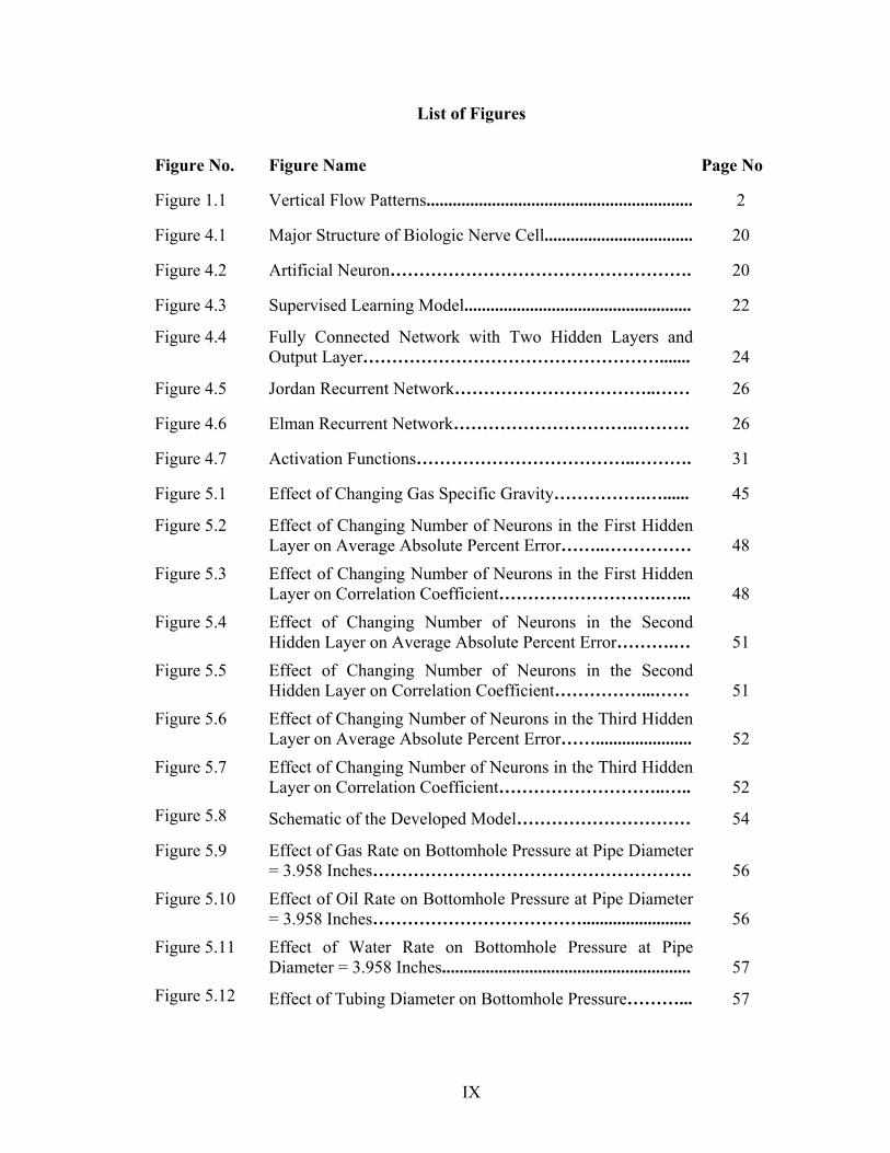
List of Figures
Figure No. Figure Name Page No
Figure 1.1 Vertical Flow Patterns............................................................. 2
Figure 4.1 Major Structure of Biologic Nerve Cell.................................. 20
Figure 4.2 Artificial Neuron……………………………………………. 20
Figure 4.3 Supervised Learning Model.................................................... 22
Figure 4.4 Fully Connected Network with Two Hidden Layers and Output Layer…………………………………………….......
24
Figure 4.5 Jordan Recurrent Network……………………………..…… 26
Figure 4.6 Elman Recurrent Network………………………….………. 26
Figure 4.7 Activation Functions………………………………..………. 31
Figure 5.1 Effect of Changing Gas Specific Gravity…………….…...... 45
Figure 5.2 Effect of Changing Number of Neurons in the First Hidden Layer on Average Absolute Percent Error……..……………
48
Figure 5.3 Effect of Changing Number of Neurons in the First Hidden Layer on Correlation Coefficient……………………….…...
48
Figure 5.4 Effect of Changing Number of Neurons in the Second Hidden Layer on Average Absolute Percent Error……….…
51
Figure 5.5 Effect of Changing Number of Neurons in the Second Hidden Layer on Correlation Coefficient……………...……
51
Figure 5.6 Effect of Changing Number of Neurons in the Third Hidden Layer on Average Absolute Percent Error……......................
52
Figure 5.7 Effect of Changing Number of Neurons in the Third Hidden Layer on Correlation Coefficient………………………..…..
52
Figure 5.8 Schematic of the Developed Model………………………… 54
Figure 5.9 Effect of Gas Rate on Bottomhole Pressure at Pipe Diameter = 3.958 Inches……………………………………………….
56
Figure 5.10 Effect of Oil Rate on Bottomhole Pressure at Pipe Diameter = 3.958 Inches……………………………….........................
56
Figure 5.11 Effect of Water Rate on Bottomhole Pressure at Pipe Diameter = 3.958 Inches.........................................................
57
Figure 5.12 Effect of Tubing Diameter on Bottomhole Pressure………... 57
X
Figure 5.13 Effect of Pipe Length on Bottomhole Pressure at Pipe Diameter = 3.958 Inches…………………………………….
58
Figure 5.14 Effect of Changing Oil Rate for Three Different Tubing Sizes…………………………………………………………
60
Figure 5.15 Effect of Changing Gas Rate for Three Different Tubing Sizes…………………………………………………………
60
Figure 5.16 Effect of Changing Water Rate for Three Different Tubing Sizes…………………………………………………………
61
Figure 5.17 Effect of Changing tubing Depth for Three Different Tubing Sizes........................................................................................
61
Figure 5.18 Statistical Accuracy of BHP Grouped by Oil Rate (with Corresponding Data Points)…………………………………
63
Figure 5.19 Statistical Accuracy of BHP Grouped by Gas Rate (with Corresponding Data Points)....................................................
63
Figure 5.20 Statistical Accuracy of BHP Grouped by Water Rate (with Corresponding Data Points)....................................................
64
Figure 5.21 Statistical Accuracy of BHP Grouped by Tubing Diameter (with Corresponding Data Points)…………………………...
64
Figure 5.22 Statistical Accuracy of BHP Grouped by Tubing Depth (with Corresponding Data Points)…………………………...
65
Figure 5.23 Crossplot of Observed Vs. Calculated BHP for Ansari et al. Model………………………………………………………..
70
Figure 5.24 Crossplot of Observed Vs. Calculated BHP for Chokshi et al. Model……………………………………………………
70
Figure 5.25 Crossplot of Observed Vs. Calculated BHP for Gomez et al. Model………………………………………………………..
71
Figure 5.26 Crossplot of Observed Vs. Calculated BHP for Beggs and Brill Correlation……………………………………………..
71
Figure 5.27 Crossplot of Observed Vs. Calculated BHP for Duns and Ros Correlation……………………………………………...
72
Figure 5.28 Crossplot of Observed Vs. Calculated BHP for Hagedorn and Brown Correlation………………………………………
72
Figure 5.29 Crossplot of Observed Vs. Calculated BHP for Mukhrejee and Brill Correlation………………………………………...
73
Figure 5.30 Crossplot of Observed Vs. Calculated BHP for Orkiszewski Correlation…………………………………………………..
73
Figure 5.31 Crossplot of Observed Vs. Calculated BHP for Hasan and Kabir Model…………………………………………………
74
XI
Figure 5.32 Crossplot of Observed Vs. Calculated BHP for Training Set (ANN Model)………………………………………………..
74
Figure 5.33 Crossplot of Observed Vs. Calculated BHP for Validation Set (ANN Model)……………………………………………
75
Figure 5.34 Crossplot of Observed Vs. Calculated BHP for Testing Set (ANN Model)………………………………………………..
75
Figure 5.35 Comparison of Correlation Coefficients for the Developed Model, Empirical Correlations, and Mechanistic Models……………………………………………………….
76 Figure 5.36 Comparison of Root Mean Squared Errors for the
Developed Model, Empirical Correlations, and Mechanistic Models……………………………………………………….
76
Figure 5.37 Comparison of AAPE for the Developed Model, other Empirical Correlations, and Mechanistic Models…….……..
80
Figure 5.38 Error Distribution for Training Set (ANN Model)………….. 80
Figure 5.39 Error Distribution for Validation Set (ANN Model)……….. 81
Figure 5.40 Error Distribution for Testing Set (ANN Model)…………... 81
Figure 5.41 Error Distribution for Ansari et al. Model………………….. 82
Figure 5.42 Error Distribution for Chokshi et al. Model………………... 82
Figure 5.43 Error Distribution for Gomez et al. Model………………… 83
Figure 5.44 Error Distribution for Beggs and Brill Correlation…………. 83
Figure 5.45 Error Distribution for Duns and Ros Correlation…………… 84
Figure 5.46 Error Distribution for Hagedorn and Brown Correlation........ 84
Figure 5.47 Error Distribution for Mukhrejee and Brill Correlation…….. 87
Figure 5.48 Error Distribution for Orkiszewski Correlation…………….. 87
Figure 5.49 Error Distribution for Hasan and Kabir Model……………... 88
Figure 5.50 Residual Graph for Ansari et al. Model…………………….. 91
Figure 5.51 Residual Graph for Chokshi et al. Model............................... 91
Figure 5.52 Residual Graph for Gomez et al. Model……………………. 92
Figure 5.53 Residual Graph for Beggs and Brill Correlation……………. 92
Figure 5.54 Residual Graph for Duns and Ros Correlation…………...… 93
XII
Figure 5.55 Residual Graph for Hagedorn and Brown Correlation……... 93
Figure 5.56 Residual Graph for Mukhrejee and Brill Correlation………. 94
Figure 5.57 Residual Graph for Orkiszewski Correlation……………….. 94
Figure 5.58 Residual Graph for Hasan and Kabir model........................... 95
Figure 5.59 Residual Graph for Training Set (ANN Model)..................... 95
Figure 5.60 Residual Graph for Validation Set (ANN Model)………….. 96
Figure 5.61 Residual Graph for Testing Set (ANN Model)……………... 96
XIII
List of Tables
Table No. Table Name Page
Table 5.1 Performance of Empirical Correlations and Mechanistic Using All Data ……………………………………………………………………
42
Table 5.2 Effect of Changing Number of Neurons in the First Hidden Layer with Resepect to Average Absolute Percent Error and Correlation Coefficient …………………………………..........................................
50
Table 5.3 Effect of Changing Number of Neurons in the Second Hidden Layer with Resepect to Average Absolute Percent Error and Correlation Coefficient ………………………………………………………...…...
50
Table 5.4 Effect of Changing Number of Neurons in the Third Hidden Layer with Resepect to Average Absolute Percent Error and Correlation Coefficient …………………………………………………......………
50
Table 5.5 Statistical Analysis Results of Empirical Correlations and Mechanistic Models………………………………………….....................................
66
Table 5.6 Statistical Analysis Results of Developed Neural Network Model........ 78
Table 5.7 Residual Limits of the New ANN Model and Best Available Empirical Correlations and Mechanistic Models ……………………...
90
1
CHAPTER 1
INTRODUCTION
Multiphase flow in pipes can be defined as the process of simultaneous flow of
two phases or more namely; liquid and gas. It occurs in almost all oil production wells, in
many gas production wells, and in some types of injection wells. This process has raised
considerable attention from nuclear and chemical engineering disciplines as well as
petroleum engineering. The phenomenon is governed mainly by bubble point pressure;
whenever the pressure drops below bubble point, gas will evolve from liquid, and from
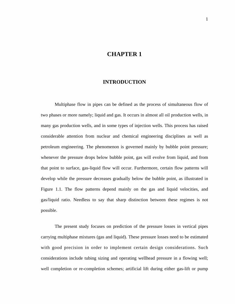
that point to surface, gas-liquid flow will occur. Furthermore, certain flow patterns will
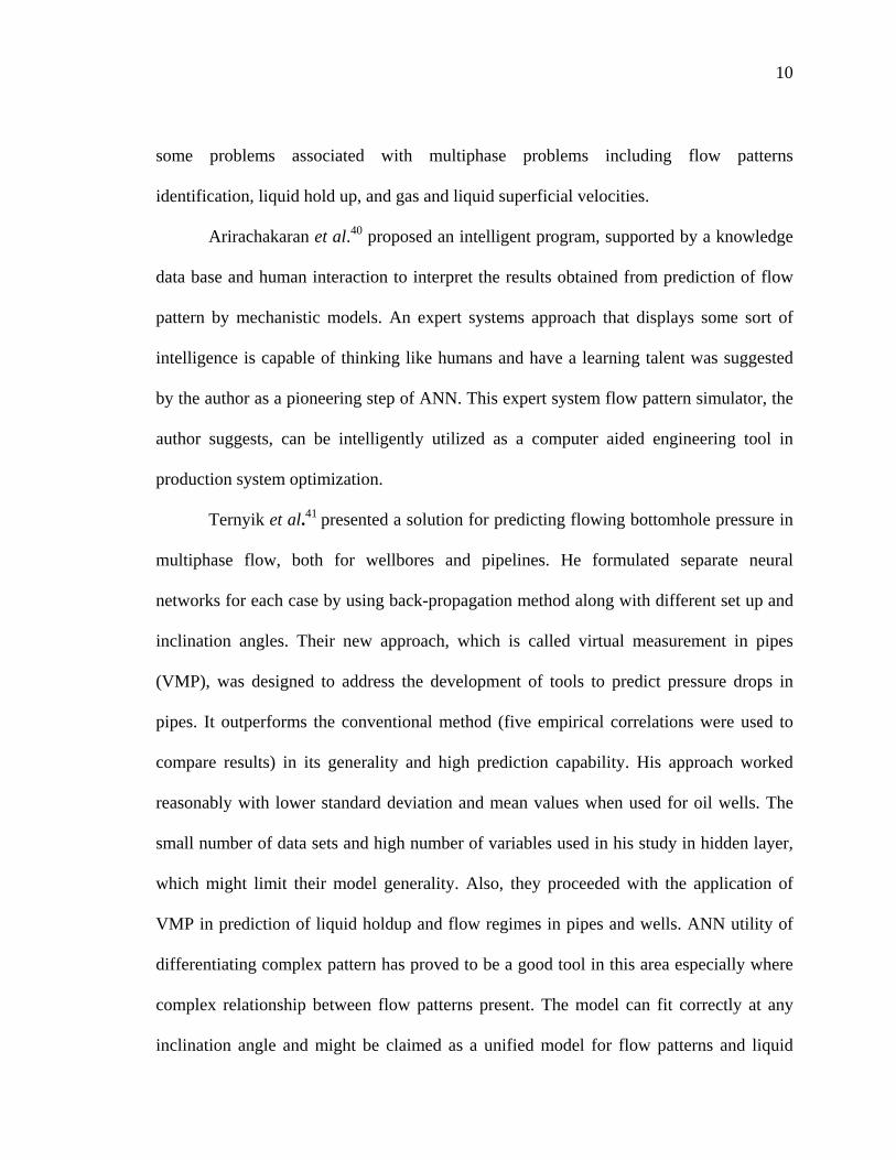
develop while the pressure decreases gradually below the bubble point, as illustrated in
Figure 1.1. The flow patterns depend mainly on the gas and liquid velocities, and
gas/liquid ratio. Needless to say that sharp distinction between these regimes is not
possible.
The present study focuses on prediction of the pressure losses in vertical pipes
carrying multiphase mixtures (gas and liquid). These pressure losses need to be estimated
with good precision in order to implement certain design considerations. Such
considerations include tubing sizing and operating wellhead pressure in a flowing well;
well completion or re-completion schemes; artificial lift during either gas-lift or pump
2
Figure 1.1: Vertical Flow Patterns.
Bubble flow
-- ---- ---- --------
-- -- -- ---- -- -- -- -- --
-- -- -- -- -- -- -- --
-- -- -- ------ ---- -- -- --
-- -- -- -- -- -- ---- -- -- -- -- -- -- -- -- -- -- -- -- -- -- -- -- -- -- -- -- -- -- -- -- -- -- -- -- --
-- -- -- -- ------ --
-- -- -- -- -- -- -- -- ------ --
-- -- -- ---- -- ---- -- -- -- --
Slug Flow Churn Flow Annular Flow

3
operation in a low energy reservoir; liquid unloading in gas wells; direct input for surface
flow line and equipment design calculations.
In the present study, Chapter 2 reviews and discusses literature relevant to the
topics addressed in this work. Chapter 3 presents the statement of the problem and defines
the general objectives. In Chapter 4 a general framework for the concept of artificial
neural networks is presented. Great emphasis is placed on a back propagation learning
algorithm that was utilized in developing a model for predicting pressure drop in
multiphase flow wells. Also, the model parameters are discussed along with general
network optimization. Chapter 5 presents the model optimization and results of the
developed model along with a comparison to the best available empirical correlations and
mechanistic models. Finally, Chapter 6 concludes and summarizes the findings of this
study and discusses potential future developments for the used approach.
4
CHAPTER 2
LITERATURE REVIEW
This chapter provides a revision of the most commonly used correlations and
mechanistic models and their drawbacks. The concept of artificial neural network is, in
brief, being presented along with its applications in petroleum industry as well as in
multiphase flow area. Special emphasis is devoted to pressure drop calculations in
multiphase flow wells using the best available empirical correlations and mechanistic
models.
2.1 Empirical Correlations
Numerous correlations have been developed since the early 1940s on the subject
of vertical multiphase flow. Most of these correlations were developed under laboratory
conditions and are, consequently, inaccurate when scaled-up to oil field conditions1. A
detailed description of these correlations is given in Appendix A for reference. The most
commonly used correlations are those of Hagedorn and Brown2, Duns and Ros3,
Orkiszewski4, Beggs and Brill5, Aziz and Govier6, and Mukherjee and Brill7. These
correlations, discussed in Appendix A, have been evaluated and studied carefully by
numerous researchers to validate their applicability under different ranges of data.
5
Espanol8 has shown that Orkiszewski4 correlation was found more accurate than
other correlations in determining pressure drop especially when three-phase flow is
introduced in wellbores.
Camacho9 collected data from 111 wells with high gas-liquid ratios to test five
correlations. None of these wells encountered a mist flow regime defined by Duns and
Ros3 or Orkiszewski4 correlations. He reported that no single method was sufficiently
accurate to cover all ranges of gas-liquid ratios. Duns and Ros3 and Orkiszewski4
correlations performed better when forced to mist flow for gas liquid ratios exceed 10,000
SCF/STB.
Messulam10 has also conducted a comparative study using data from 434 wells to
test the performance of available correlations. Six methods were tested and no one was
found to be superior for all data ranges. Hagedorn and Brown2 followed by Orkiszewski4
correlation were the most accurate over the other tested methods. Duns and Ros3 method
was the least accurate one.
Lawson and Brill11 presented a study to ascertain the accuracy of seven pressure-
loss prediction methods. The best method was Hagedorn and Brown2 followed by
Orkiszewski4 correlation.
The same number of field data points (726, used by Lawson and Brill11) was used
by Vohra et al.12. The purpose of their study was to include the new methods of Beggs
and Brill5, Aziz et al.6, and Chierici et al.13. It was found that Aziz et al.6 performed the
best followed by the Beggs and Brill5 and Chierici et al.13 correlations.
Chierici et al.13 proposed a new method to be used in slug flow regime only. They
suggested using the Griffith and Wallis14 correlation in bubble flow and the Duns and

6
Ros3 method in mist flow. Besides, they specified which fluid property correlations have
to be used for calculating two-phase flowing pressure gradients by their method. The
Vohra et al.12 study showed that this method overestimates pressure drop calculation in
most cases.
Several correlations have been investigated using about 115 field data points by
Kabir et al.15. Their correlation performed better than Aziz et al.6 and Orkiszweski4
correlations, when the slug and bubble flows are predominant. They claimed also that
their correlation is outperforming the rest of correlations in the churn and annular flow
regimes.
Aggour et al.16 evaluated the performance of vertical multiphase flow correlations
and the possibility of applying those set of correlations for conditions in Gulf region
where large tubular and high flow rates are dominant. They concluded that Beggs and
Brill5 correlation outperforms the rest of correlations in pressure prediction. Hagedorn and
Brown2 correlation was found to be better for water cuts greater than 80%. Also, they
reported that Aziz et al.6 correlation could be improved when Orkiszewski flow pattern is
applied.
Bharath17 reported that the Orkiszewski4 and Hagedorn and Brown2 correlations
are found to perform satisfactorily for vertical wells with or without water cut. Also, He
concluded that Duns and Ros3 correlation is not applicable for wells with water-cut and
should be avoided for such cases. The Beggs and Brill5 correlation is applicable for
inclined wells with or without water-cut and is probably the best choice available for
deviated wells.

7
Most researchers agreed upon the fact that no single correlation was found to be
applicable over all ranges of variables with suitable accuracy1. It was found that
correlations are basically statistically derived, global expressions with limited physical
considerations, and thus do not render them to a true physical optimization
2.2 Mechanistic Models
Mechanistic models are semi-empirical models used to predict multiphase flow
characteristics such as liquid hold up, mixture density, and flow patterns. Based on sound
theoretical approach, most of these mechanistic models were generated to outperform the
existing empirical correlations.
Four mechanistic models will be reviewed in this study; those of Hasan and
Kabir15, Ansari et al.18, Chokshi et al.19, and Gomez et al.20. Detailed description of these
models is provided in Appendix A.
Hasan and Kabir15 and Ansari et al.18 models were evaluated thoroughly by
Pucknell et al.21 who reported that Hasan and Kabir15 model was found to be no better
than the traditional correlations while Ansari et al. model18 gave reasonable accuracy.
Kaya et al.22 have proposed another comprehensive mechanistic model for predicting flow
patterns in inclined upward and vertical pipes with five flow patterns used; bubbly,
dispersed, bubble, slug, churn and annular flows. Their model was tested against four
mechanistic models and two empirical correlations and was found to perform better than
the rest. These different flow patterns are definitely resulting from the changing form of
the interface between the two phases.

8
Tengesdal et al.23 did the same as Kaya et al.22, they identified five flow patterns
and came up with vertical upward two-phase flow mechanistic model for predicting these
flow patterns and liquid hold up plus pressure drop. He developed a new model for churn
flow pattern and utilized some famous mechanistic model for the rest of flow regimes.
The model also tested and gave satisfactory result compared to different schemes.
Generally, each of these mechanistic models has an outstanding performance in specific
flow pattern prediction and that is made the adoption for certain model of specific flow
pattern by investigators to compare and yield different, advanced and capable mechanistic
models.
Takacs1 made a statistical study on the possible source errors in empirical
correlation and mechanistic models. He concluded that there is no pronounced advantage
for mechanistic models over the current empirical correlations in pressure prediction
ability when fallacious values are excluded. Actually, there is no privilege for mechanistic
models over the existing empirical correlation but they behave similarly when mistaken
data from the former is taken out.
2.3 Artificial Neural Networks
Artificial neural networks are collections of mathematical models that emulate
some of the observed properties of biological nervous systems and draw on the analogies
of adaptive biological learning. The concept of artificial neural network and how it works
will be discussed in details in chapter 4.
9
2.3.1 The Use of Artificial Neural Networks in Petroleum Industry
The use of artificial intelligence in petroleum industry can be tracked back just
almost ten years24. The use Artificial Neural Network (ANN) in solving many petroleum
industry problems was reported in the literature by several authors.
Conventional computing tools have failed to estimate a relationship between
permeability and porosity. Knowing the behavior of this relationship is of utmost
significance for estimating the spatial distribution of permeability in the reservoirs
especially those of heterogeneous litho-facies. ANN was used successfully in determining
the relationship between them and constructing excellent prediction or estimation25. For
instance; ANN has a great share in solving problems related to drilling such as drill bit
diagnosis and analysis25, 26, 27, 28. Moreover, ANN was used efficiently to optimize
production, fracture fluid properties30.
ANN has also been adopted in several other areas such as permeability
predictions30, well testing31, 32, 33, reservoir engineering and enhance oil recovery
specifically34; PVT properties prediction35, 36, 37, identification of sandstone lithofacies,
improvement of gas well production38, prediction and optimization of well performance,
and integrated reservoir characterization and portfolio management39.
2.3.2 Artificial Neural Networks in Multiphase Flow
Recently, ANN has been applied in the multiphase flow area and achieved
promising results compared to the conventional methods (correlations and mechanistic
models). With regard to this field, a few researchers applied ANN technique to resolve
10
some problems associated with multiphase problems including flow patterns
identification, liquid hold up, and gas and liquid superficial velocities.
Arirachakaran et al.40 proposed an intelligent program, supported by a knowledge
data base and human interaction to interpret the results obtained from prediction of flow
pattern by mechanistic models. An expert systems approach that displays some sort of
intelligence is capable of thinking like humans and have a learning talent was suggested
by the author as a pioneering step of ANN. This expert system flow pattern simulator, the
author suggests, can be intelligently utilized as a computer aided engineering tool in
production system optimization.
Ternyik et al.41 presented a solution for predicting flowing bottomhole pressure in
multiphase flow, both for wellbores and pipelines. He formulated separate neural
networks for each case by using back-propagation method along with different set up and
inclination angles. Their new approach, which is called virtual measurement in pipes
(VMP), was designed to address the development of tools to predict pressure drops in
pipes. It outperforms the conventional method (five empirical correlations were used to
compare results) in its generality and high prediction capability. His approach worked
reasonably with lower standard deviation and mean values when used for oil wells. The
small number of data sets and high number of variables used in his study in hidden layer,
which might limit their model generality. Also, they proceeded with the application of
VMP in prediction of liquid holdup and flow regimes in pipes and wells. ANN utility of
differentiating complex pattern has proved to be a good tool in this area especially where
complex relationship between flow patterns present. The model can fit correctly at any
inclination angle and might be claimed as a unified model for flow patterns and liquid
11
hold up prediction. Mukherjee42 experimental data set was used due to wide coverage of
inclination angles reported in to provide more generality and confidence to the output
results. A Kohonen type network was utilized due to the ability of this network to self
learning without depending on the output in each case. His model was restricted to a 1.5
inch tubing diameter and low operating condition, which limit the generality of his model.
The need for accurate hold up and flow patterns prediction stimulated Osman43 to
propose an artificial neural networks model for accurate prediction of these two variables
under different conditions. 199-data points were used to construct his model. Neural
Network performed perfectly in predicting liquid hold up in terms of lowest standard
deviation and average absolute percent error when compared to published models. His
model did not work efficiently in the transition phases.
Osman and Aggour44 presented an artificial neural networks model for predicting
pressure drop in horizontal and near-horizontal multiphase flow. A three-layer back-
propagation ANN model was developed using a wide range of data. Thirteen variables
were considered as the most effective variables incorporated in pressure drop prediction.
Their model achieved outstanding performance when compared to some of the existing
correlations and two mechanistic models. The model was also found to correctly simulate
the physical process.
Shippen et al.45 confirmed the use of ANN as a good tool to predict liquid hold up
in two phase horizontal flow. The author discussed the inapplicability of current
mechanistic models and empirical correlation and the superiority of ANN over them.
Large set of data was used to provide high degree of generality to their model. Highest

12
correlation factor (0.985), compared to cases tested, indicates the superior overall
performance of the model.
As stated by different authors and researchers, and as discussed earlier, the
empirical correlations and mechanistic models failed to provide a satisfactorily and a
reliable tool for estimating pressure in multiphase flow wells. High errors are usually
associated with these models and correlations which encouraged a new approach to be
investigated for solving this problem. Artificial neural networks gained wide popularity in
solving difficult and complex problems, especially in petroleum engineering. This new
approach will be utilized for the first time in solving the problem of estimating pressure
drop for multiphase flow in vertical oil wells.

13
CHAPTER 3
STATEMENT OF THE PROBLEM AND OBJECTIVES
This chapter describes the problem of estimating pressure drop for vertical
multiphase flow in oil wells. The need for developing a model that can overcome the
previous difficulties faced in utilizing empirical correlations and mechanistic models is
addressed through stating the objective of this work.
3.1 Statement of the Problem
The need for accurate pressure prediction in vertical multiphase is of great
importance in the oil industry. Prediction of pressure drop is quite difficult and
complicated due to the complex relationships between the various parameters involved.
These parameters include pipe diameter, slippage of gas past liquid, fluid properties, and
the flow rate of each phase. Another parameter, which adds to the difficulty, is the flow
patterns and their transition boundaries inside the wellbore along with changing
temperature and pressure conditions. Therefore, an accurate analytical solution for this
problem is difficult or impossible to achieve. However, numerous attempts have been
tried since the early fifties to come up with precise methods to estimate pressure drop in
vertical multiphase flow. These attempts varied from empirical correlations to semi
empirical (mechanistic models) approaches. The first approach was based on development
of empirical correlations from experimental data. The second approach was based on
14
fundamental physical laws, hence, provided some sort of reliability. As discussed in
chapter 2, both solutions did not provide satisfactory and adequate results in all
conditions.
Application of Artificial Neural Network (ANN) in solving difficult problems has
gained wide popularity in the petroleum industry. This technique has the ability to
acquire, store, and utilize experiential knowledge. Besides, it can differentiate, depending
on the training data set, between complex patterns if it is well trained.
In this study, an artificial neural network model for prediction of pressure drop in
vertical multiphase flow is developed and tested against field data. Some of the best
available empirical correlations and mechanistic models are reviewed carefully using
graphical and statistical analysis. These mechanistic models and empirical correlations are
compared against the generated artificial neural network model.
3.2 Objective
The general objective of this study is to develop an artificial neural network model
that provides more accurate prediction of pressure drop in vertical multiphase flow. Data
from different Middle Eastern fields are used in this study. Specific objectives are:
1. To construct an ANN model for predicting pressure drop in vertical multiphase
flow.
2. To test the constructed model against actual field data.
3. To compare the developed model against the best available empirical correlations
and mechanistic models.

15
CHAPTER 4
NEURAL NETWORKS
This chapter deals with addressing the concept of artificial neural networks. First,
historical background will be introduced, then, the fundamentals of ANN along with a
deep insight to the mathematical representation of the developed model and the network
optimization and configuration will be also discussed in details. The relationship between
the mathematical and biological neuron is also explained. Besides, the way on how
network functions is addressed through defining network structure, which deals also with
solving many problems encountered during establishment of the model. Finally, the
chapter concludes with presenting the robust learning algorithm that used in the training
process.
4.1 Artificial Intelligence
The science of artificial intelligence or what is synonymously known as soft
computing shows better performance over the conventional solutions. Sage46 defined the
aim of artificial intelligence as the development of paradigms or algorithms that require
machines to perform tasks that apparently require cognition when performed by humans.
This definition is widely broadened to include preceptrons, language, and problems
16
solving as well as conscious, unconscious processes47. Many techniques are classified
under the name of artificial intelligence such as genetic algorithms, expert systems, and
fuzzy logic because of their ability, one at least, to make certain reasoning, representation,
problem solving, and generalization. Artificial neural network is also considered one of
the important components of artificial intelligence system.
4.1.1 Artificial Neural Network
4.1.1.1 Historical Background
The research has been carried on neural network can be dated back to early 1940s.
Specifically, McCulloch and Pitts48 have tried to model the low-level structure of
biological brain system. Hebb49 published the book entitled “the organization of
behavior” in which he focused mainly towards an explicit statement of a physiological
learning rule for synaptic modification. Also, he proposed that the connectivity of the
brain is continually changing as an organism learns differing functional tasks, and the
neural assemblies are created by such changes. The book was a source of inspiration for
the development of computational models of learning and adaptive systems.
However, Ashby50 published another book entitled “design for a brain; the origin
of adaptive behavior”. The book focused on the basic notion that the adaptive behavior is
not inborn but rather learned. The book emphasized the dynamic aspects of living
organism as a machine and the related concepts of stability. While Gabor51 proposed the
idea of nonlinear adaptive filters. He mentioned that learning was accomplished in these
filters through feeding samples of stochastic process into the machine, together with the
target function that the machine was expected to produce. After 15 years of McCulloch
17
and Pitts48 paper, a new approach to the pattern recognition problem was introduced by
Rosenblatt53 through what’s called later, preceptrons. The latter, at the time when
discovered, considered as an ideal achievement and the associative theorem “preceptron
convergence theorem” was approved by several authors. The preceptron is the simplest
form of a neural network that has been used for classifying patterns
This achievement followed by the introduction of LMS “least mean square
algorithm” and Adaline “adaptive linear element” that followed by Madaline “multiple-
Adaline” in 1962. Minskey and Papert53 showed that there are several problems can not
be solved by the theorem approved by Rosenblatt52 and therefore countless effort to make
such type of improvement will result in nothing. A decade of dormancy in neural network
research was witnessed because of the Minskey’s paper53 results. In 1970s, a competition
learning algorithm was invented along with incorporation of self organizing maps. Since
that time, several networks and learning algorithms were developed. A discovery of back-
propagation learning algorithm was one of these fruitful revolutions that developed by
Rumelhart et al.54.
4.1.1.2 Definition
Generally, ANN is a machine that is designed to model the way in which the brain
performs a particular task or function of interest. The system of ANN has received
different definitions55. A widely accepted term is that adopted by Alexander and
Morton56: “A neural network is a massively parallel distributed processor that has a
natural propensity for storing experiential knowledge and making it available for use”.
ANN resembles the brain in two aspects; knowledge is acquired by the network through a
18
learning process, and the interneuron connection strengths known as synaptic weights are
used to store the knowledge55. In other way, neural networks are simply a way of mapping
a set of input variables to a set of output variables through a typical learning process. So,
it has certain features in common with biological nervous system. The relationship
between the two systems and the brain system mechanism is further explained in the next
subsection.
4.1.1.2.1 Brain system
Human brain is a highly complex, nonlinear, and parallel information-processing
system. It has the capability of organizing biological neurons in a fashion to perform
certain tasks. In terms of speed, neurons are five to six orders of magnitude slower that
silicon logic gates. However, human brain compensate for this shortcoming by having a
massive interconnection between neurons. It is estimated that human brain consists of 10
billion neurons and 60 trillion synapses57. These neurons and synapses are expected to
grow and increase in both number and connection over the time through learning.
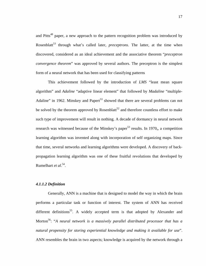
Figure 4.1 is a schematic representation of biologic nerve cell. The biological
neuron is mainly composed of three parts; dendrite, the soma, and the axon. A typical
neuron collects signals from others through a host of fine structure (dendrite). The soma
integrates its received input (over time and space) and thereafter activates an output
depending on the total input.
The neuron sends out spikes of electrical activity through a long, thin stand known
as an axon, which splits into thousands of branches (tree structure). At the end of each
branch, a synapse converts the activity from the axon into electrical effects that inhibit or

19
excite activity in the connected neurons. Learning occurs by changing the effectiveness of
synapses so that the influence of one neuron on another changes. Hence, artificial neuron
network, more or less, is an information processing system that can be considered as a
rough approximation of the above mentioned biological nerve system.
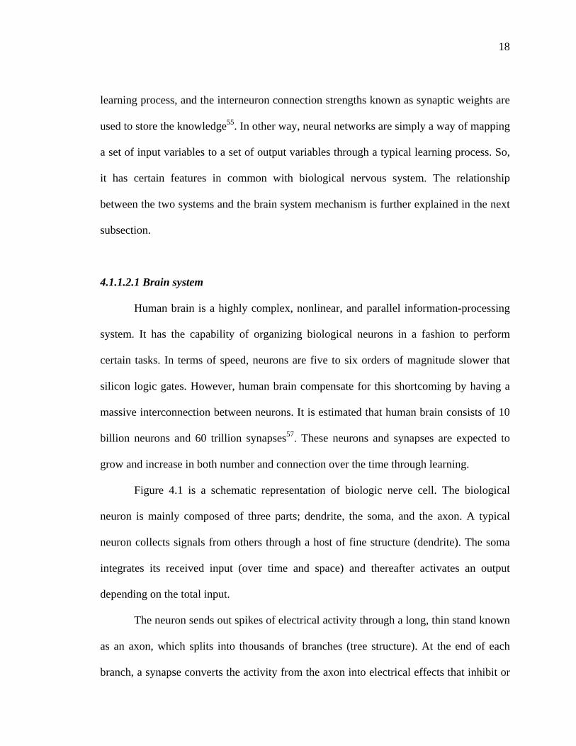
Figure 4.2 shows a typical neuron in an artificial neuron network. This
mathematical neuron is a much simpler than the biological one; the integrated information
received through input neurons take place only over space.
Output from other neurons is multiplied by the corresponding weight of the
connection and enters the neuron as an input; therefore, an artificial neuron has many
inputs and only one output. All signals in a neural network are typically normalized to
operate within certain limit. A neuron can have a threshold level that must be exceeded
before any signal is passed. The net input of the activation function may be increased by
employing a bias term rather than a threshold; the bias is the negative of threshold. The
inputs are summed and therefore applied to the activation function and finally the output
is produced51.
4.2 Fundamentals
In this section, artificial neural network basics will be presented, along with the close
relationship between the technology and the biological nervous system. A full
mathematical notation of the developed model and the network topology are also
provided.
20
AXON
TREE STRUCTURE
SOMADENDRITES
Figure 4.1: Major Structure of Biologic Nerve Cell (after Freeman58). F
F
Figure 4.2: Artificial Neuron (after Freeman58).
W1
W2
Wi
I2
.
.
.
.Ii
iW
j
i iI∑
= 1
I1

21
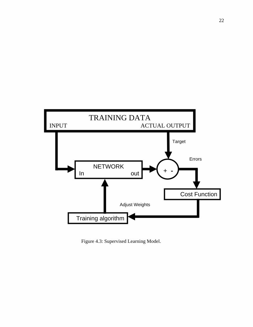
4.2.1 Network Learning
The network is trained using supervised learning “providing the network with
inputs and desired outputs”. The difference between the real outputs and the desired
outputs is used by the algorithm to adapt the weights in the network. Figure 4.3 illustrates
the supervised learning diagram. The net output is calculated and compared with the
actual one, if the error between the desired and actual output is within the desired
proximity, there will be no weights' changes; otherwise, the error will be back-propagated
to adjust the weights between connections (feed backward cycle). After the weights are
fixed the feed forward cycle will be utilized for the test set.
The other learning scheme is the unsupervised one where there is no feedback from the
environment to indicate if the outputs of the network are correct. The network must
discover features, rules, correlations, or classes in the input data by itself. As a matter of
fact, for most kinds of unsupervised learning, the targets are the same as inputs. In other
words, unsupervised learning usually performs the same task as an auto-associative
network, compressing the information from the inputs.
4.2.2 Network Architecture
Network topology (architecture) is an important feature in designing a successful
network. Typically, neurons are arranged in layers, each layer is responsible for
performing a certain task. Based on how interconnections between neurons and layers are;
neural network can be divided into two main categories (feed forward and recurrent).
22
Figure 4.3: Supervised Learning Model.
+ -
TRAINING DATA INPUT ACTUAL OUTPUT
Cost Function
Training algorithm
NETWORK In out
Adjust Weights
Target
Errors
23
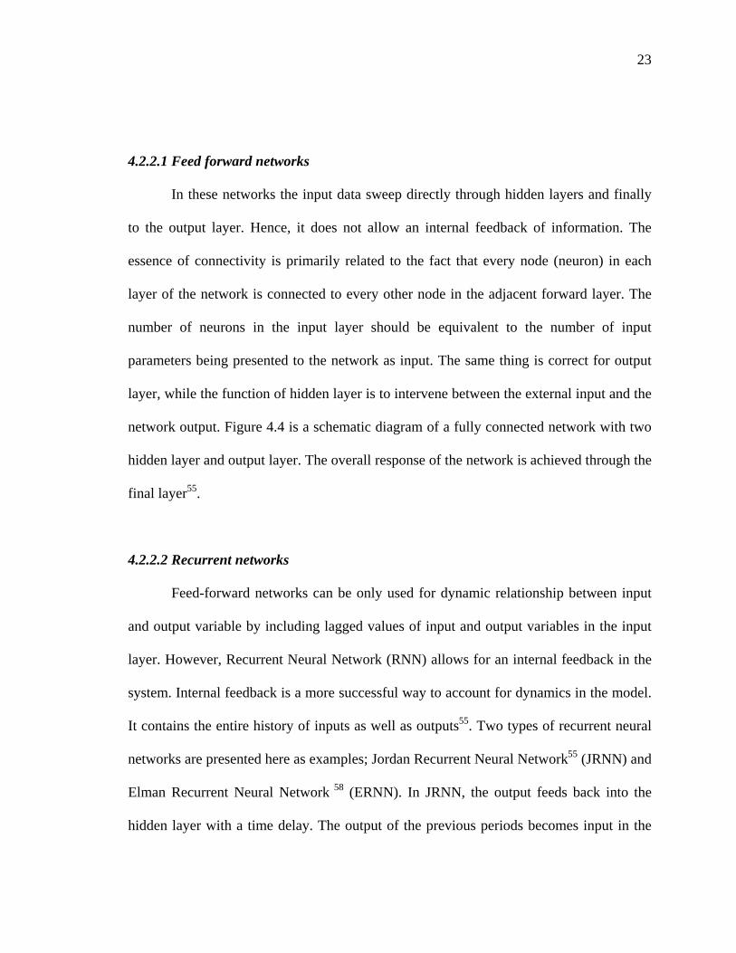
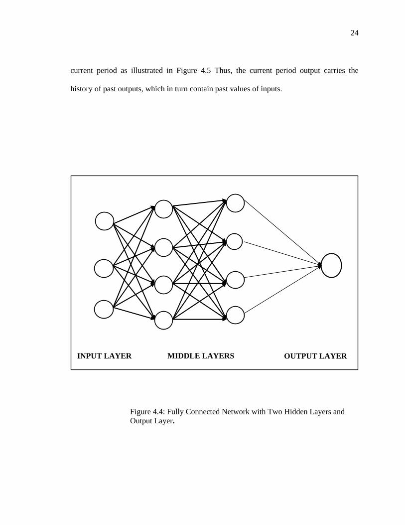
4.2.2.1 Feed forward networks
In these networks the input data sweep directly through hidden layers and finally
to the output layer. Hence, it does not allow an internal feedback of information. The
essence of connectivity is primarily related to the fact that every node (neuron) in each
layer of the network is connected to every other node in the adjacent forward layer. The
number of neurons in the input layer should be equivalent to the number of input
parameters being presented to the network as input. The same thing is correct for output
layer, while the function of hidden layer is to intervene between the external input and the
network output. Figure 4.4 is a schematic diagram of a fully connected network with two
hidden layer and output layer. The overall response of the network is achieved through the
final layer55.
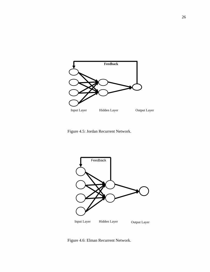
4.2.2.2 Recurrent networks
Feed-forward networks can be only used for dynamic relationship between input
and output variable by including lagged values of input and output variables in the input
layer. However, Recurrent Neural Network (RNN) allows for an internal feedback in the
system. Internal feedback is a more successful way to account for dynamics in the model.
It contains the entire history of inputs as well as outputs55. Two types of recurrent neural
networks are presented here as examples; Jordan Recurrent Neural Network55 (JRNN) and
Elman Recurrent Neural Network 58 (ERNN). In JRNN, the output feeds back into the
hidden layer with a time delay. The output of the previous periods becomes input in the
24
current period as illustrated in Figure 4.5 Thus, the current period output carries the
history of past outputs, which in turn contain past values of inputs.
Figure 4.4: Fully Connected Network with Two Hidden Layers and Output Layer.
INPUT LAYER MIDDLE LAYERS OUTPUT LAYER
25
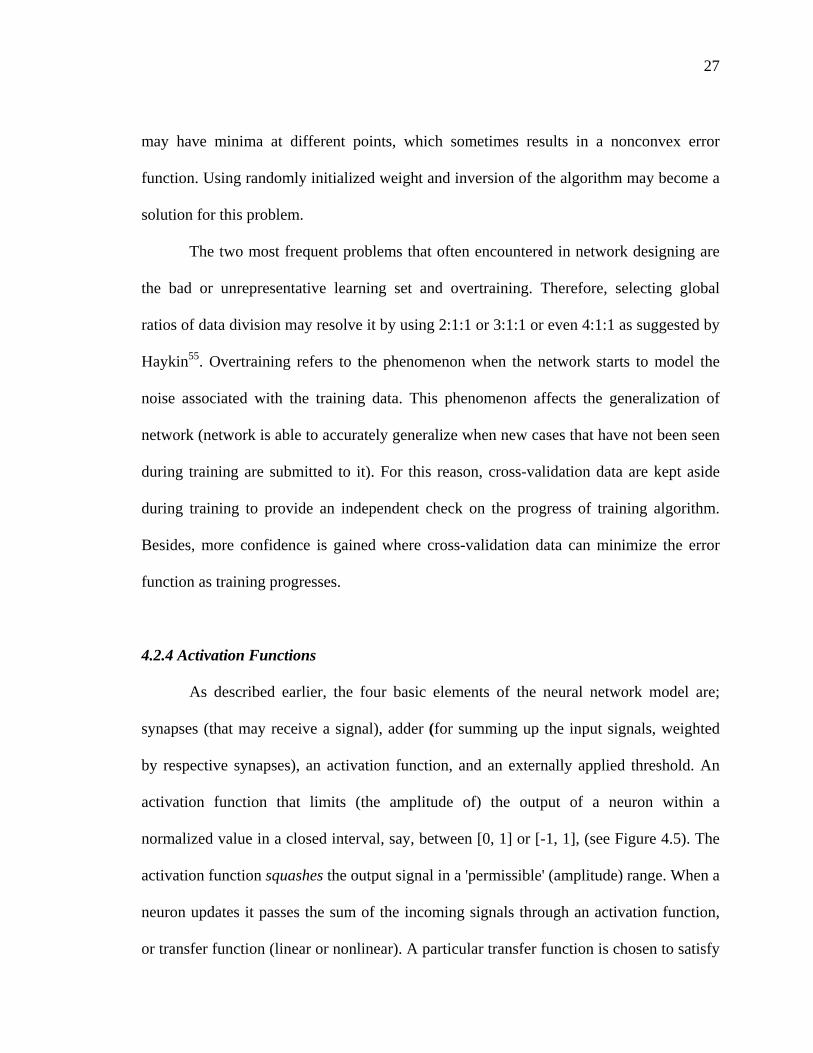
While a two-layer Elman Recurrent Neural Network (ERNN) is depicted in Figure
4.6. The ERNN accounts for internal feedback in such a way that the hidden layer output
feeds back in itself with a time delay before sending signals to the output layer. RNN,
however, requires complex computational processes that can only be performed by more
powerful software. The back-propagation algorithm is used during the training process in
the computation of estimates of parameters.
4.2.3 General Network Optimization
Any network should be well optimized in different senses in order to simulate the
true physical behavior of the property under study. Certain parameters can be well
optimized and rigorously manipulated such as selection of training algorithm, stages, and
weight estimation. An unsatisfactory performance of the network can be directly related
to an inadequacy of the selected network configuration or when the training algorithm
traps in a local minimum or an unsuitable learning set.
In designing network configuration, the main concern is the number of hidden
layers and neurons in each layer. Unfortunately, there is no sharp rule defining this feature
and how it can be estimated. Trial and error procedure remains the available way to do so,
while starting with small number of neurons and hidden layers “and monitoring the
performance” may help to resolve this problem efficiently. Regarding the training
algorithms, many algorithms are subjected to trapping in local minima where they stuck
on it unless certain design criteria are modified. The existence of local minima is due to
the fact that the error function is the superposition of nonlinear activation functions that
26
Figure 4.5: Jordan Recurrent Network.
Figure 4.6: Elman Recurrent Network.
Input Layer Hidden Layer Output Layer
Feedback
Input Layer Hidden Layer Output Layer
Feedback
27
may have minima at different points, which sometimes results in a nonconvex error
function. Using randomly initialized weight and inversion of the algorithm may become a
solution for this problem.
The two most frequent problems that often encountered in network designing are
the bad or unrepresentative learning set and overtraining. Therefore, selecting global
ratios of data division may resolve it by using 2:1:1 or 3:1:1 or even 4:1:1 as suggested by
Haykin55. Overtraining refers to the phenomenon when the network starts to model the
noise associated with the training data. This phenomenon affects the generalization of
network (network is able to accurately generalize when new cases that have not been seen
during training are submitted to it). For this reason, cross-validation data are kept aside
during training to provide an independent check on the progress of training algorithm.
Besides, more confidence is gained where cross-validation data can minimize the error
function as training progresses.
4.2.4 Activation Functions
As described earlier, the four basic elements of the neural network model are;
synapses (that may receive a signal), adder (for summing up the input signals, weighted
by respective synapses), an activation function, and an externally applied threshold. An
activation function that limits (the amplitude of) the output of a neuron within a
normalized value in a closed interval, say, between [0, 1] or [-1, 1], (see Figure 4.5). The
activation function squashes the output signal in a 'permissible' (amplitude) range. When a
neuron updates it passes the sum of the incoming signals through an activation function,
or transfer function (linear or nonlinear). A particular transfer function is chosen to satisfy
28
some specification of the problem that the neuron is attempting to solve. In mathematical
terms, a neuron j has two equations that can be written as follows55:
)2.4(..................................................................................... )(
)1.4(...................................................................................... 1
pjNETpjyand
N
i pixjiwpjNET
φϕ −=
∑=
=
Where; xp1, xp2, ..…, xpN are the input signals; wj1, wj2, …, wjk are the synaptic weights of
neuron j; NETpj is the linear combiner output, pjφ is the threshold, ϕ is the activation
function; and ypj is the output signal of the neuron.
Four types of activation functions are identified based on their internal features. A simple
threshold function has a form of:
)3.4(.............................................................................................)( pjNETkpjy =
Where k is a constant threshold function, i.e.:
pjy = 1 if pjNET )( > T
pjy = 0 otherwise.
T is a constant threshold value, or a function that more accurately simulates the
nonlinear transfer characteristics of the biological neuron and permits more general
network functions as proposed by McCulloch-Pitts model48. However, this function is not
widely used because it is not differentiable.
The second type of these transfer functions is the Gaussian function, which can be
represented as:
29
)4.4(..........................................................................................2
2
⎟⎟⎟
⎠
⎞
⎜⎜⎜
⎝
⎛
=
−
σ
pjNET
cepjy
Where:
σ is the standard deviation of the function.
The third type is the Sigmoid Function, which is being tried in the present study
for its performance. It applies a certain form of squashing or compressing the range of
pjNET )( to a limit that is never exceeded by pjy this function can be represented
mathematically by:
)5.4(............................................................... ..................
1
1
⎟⎟
⎠
⎞
⎜⎜
⎝
⎛ ×−+
=pjNETa
epjy
Where;
a is the slope parameter of the sigmoid function.
By varying the slope parameter, different sigmoid function slopes are obtained. Another
commonly used activation function is the hyperbolic function, which has the
mathematical form of:
)6.4(.........................................................................
1
1)tanh(⎟⎟⎟⎟
⎠
⎞
⎜⎜⎜⎜
⎝
⎛
−+
−−
==pjNET
e
pjNETexpjy
This function is symmetrically shaped about the origin and looks like the sigmoid
function in shape. However, this function produced good performance when compared to
30
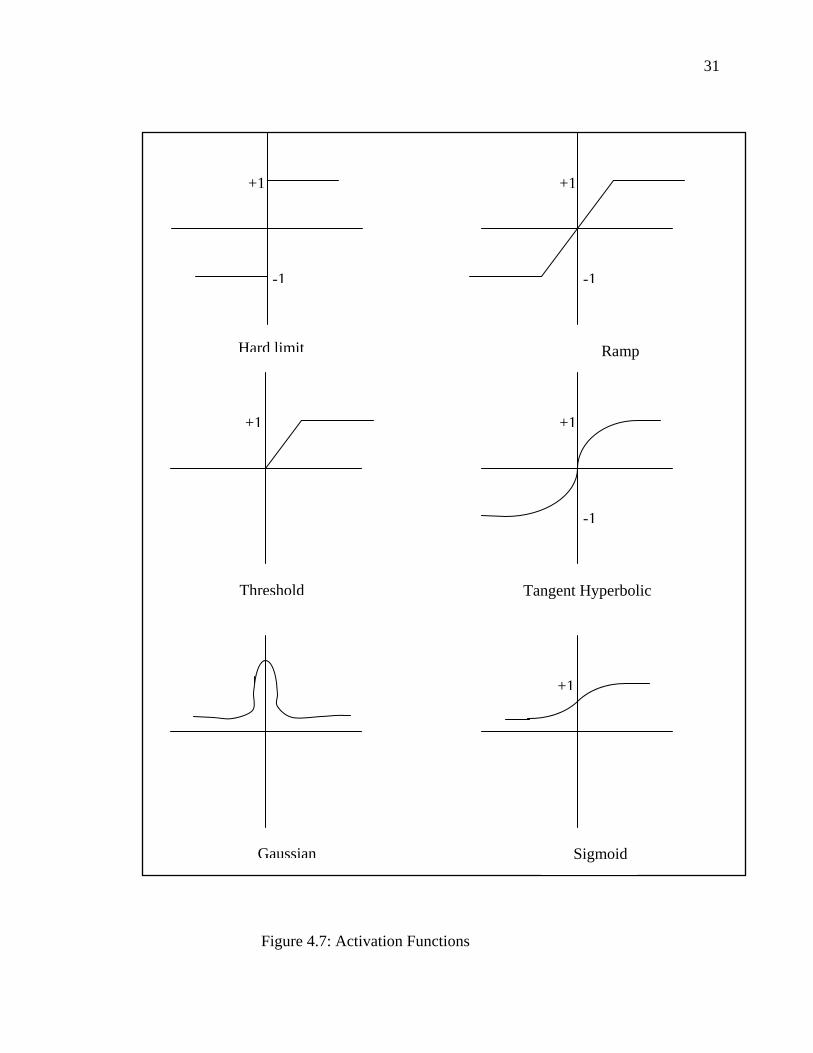
sigmoid function. Hence, it is used as an activation function for the present model. Other
functions are presented in Figure 4.7.
4.3 Back-Propagation Training Algorithm
Is probably the best known, and most widely used learning algorithm for neural
networks. It is a gradient based optimization procedure. In this scheme, the network learns
a predefined set of input-output sample pairs by using a two-phase propagate-adapt cycle.
After the input data are provided as stimulus to the first layer of network unit, it is
propagated through each upper layer until an output is generated. The latter, is then
compared to the desired output, and an error signal is computed for each output unit.
Furthermore, the error signals are transmitted backward from the output layer to each
node in the hidden layer that mainly contributes directly to the output.
However, each unit in the hidden layer receives only a portion of the total error
signal, based roughly on the relative contribution the unit made to the original output.
This process repeats layer by layer, until each node in the network has received an error
signal that describes its relative contribution to the total error. Based on the error signal
received, connection weights are then updated by each unit to cause the network to
converge toward a state that allows all the training set to be prearranged. After training,
different nodes learn how to recognize different features within the input space. The way
of updating the weights connections is done through the generalized delta rule "GDR". A
full mathematical notion is presented in the next subsection.
31
Figure 4.7: Activation Functions
Hard limit Ramp
Threshold Tangent Hyperbolic
Gaussian Sigmoid
+1
+1 +1
-1
+1
-1
+1
-1
32
4.3.1 Generalized Delta Rule
This section deals with the formal mathematical expression of Back-Propagation
Network operation. The learning algorithm, or generalized delta rule, and its derivation
will be discussed in details. This derivation is valid for any number of hidden layers.
Suppose the network has an input layer that contains an input vector;
( ) )7.4.(................................................................................,...,,, 321t
pNpppp xxxxx =
The input units distribute the values to the hidden layer units. The net output to the j th
hidden unit is:
)8.4......(................................................................................1∑=
+=N
i
hjpi
hji
hpj xwNET θ
Where;
hjiw is the weight of the connection from the i th input unit, and
hjθ is the bias term
h is a subscript refer to the quantities on the hidden layer.
Assuming that the activation of this node is equal to the net input; then the output of this
node is
( ) )8.4(....................................................................................................hpj
hjpj NETfi =
The equations for the output nodes are:
)10.4........(................................................................................1∑=
+=L
j
okpj
okj
opk iwNET θ

33
( ) )11.4.......(..........................................................................................opk
okpk NETfo =
Where:
o superscript refers to quantities of the output layer unit.
The basic procedure for training the network is embodied in the following description:
1. Apply an input vector to the network and calculate the corresponding output
values.
2. Compare the actual outputs with the correct outputs and determine a measure of
the error.
3. Determine in which direction (+ or -) to change each weight in order to reduce the
error.
4. Determine the amount by which to change each weight.
5. Apply the correction to the weights.
6. Repeat steps 1 to 5 with all the training vectors until the error for all vectors in the
training set is reduced to an acceptable tolerance.
4.3.1.1 Update of Output-Layer Weights
The general error for the kth input vector can be defined as;
( ) 12).......(4........................................................................................... kkk yd −=ε
Where:
kd = desired output
ky = actual output
34
Because the network consists of multiple units in a layer; the error at a single output unit
will be defined as
( ) ...(4.13).......................................................................................... pkpkpk oy −=δ
Where;
p subscript refers to the pth training vector
k subscript refers to the kth output unit
So,
pky = desired output value from the kth unit.
pko = actual output value from the kth unit.
The error that is minimized by the GDR is the sum of the squares of the errors for all
output units;
)14.4.......(..........................................................................................21
1
2∑=
=M
kpkpE δ
To determine the direction in which to change the weights, the negative of the gradient of
pE and pE∇ , with respect to the weights, kjw should be calculated.
The next step is to adjust the values of weights in such a way that the total error is
reduced.
From equation (4.14) and the definition of pkδ , each component of pE∇ can be
considered separately as follows;
( ) )15.4.....(................................................................................21 2∑ −=
kpkpkp oyE
and
35
( ) ( )( )
)16.4(.......................................................... okj
opk
opk
ok
pkpkokj
p
wNET
NETf
oywE
∂
∂
∂∂
−−=∂
∂
The chain rule is applied in equation (4.16)
The derivative of okf will be denoted as /o
kf
( ))17.4.....(............................................................
1pj
L
j
okpj
okjo
kjokj
opk iiw
wwNET
=+∂∂
=∂
∂∑=
θ
Combining equations (4.16) and (4.17) yields the negative gradient as follows
( ) ( ) )18.4........(............................................................/pj
opk
okpkpko
kj
p iNETfoywE
−=∂
∂−
As far as the magnitude of the weight change is concerned, it is proportional to the
negative gradient. Thus, the weights on the output layer are updated according to the
following equation;
( ) ( ) ( ) )19.4........(......................................................................1 twtwtw okjp
okj
okj ∆+=+
Where;
( ) ( ) ( ) )20.4...(............................................................/pj
opk
okpkpk
okjp iNETfoytw −=∆ η
The factor η is called the learning-rate parameter, ( 10 ppη ).
4.3.1.2 Output Function
The output function ( )ojk
ok NETf should be differentiable as suggested in section 4.2.4.
This requirement eliminates the possibility of using linear threshold unit since the output
36
function for such a unit is not differentiable at the threshold value. Output function is
usually selected as linear function as illustrated below
( ) ( ) ..(4.21).......................................................................................... ojk
ojk
ok NETNETf =
This defines the linear output unit.
In the first case:
1/ =okf
( ) ( ) ( ) )22.4.........(............................................................1 pjpkpkokj
okj ioytwtw −+=+ η
The last equation can be used for the linear output regardless of the functional form of the
output function okf .
4.3.1.3 Update of Hidden-Layer Weights
The same procedure will be followed to derive the update of the hidden-layer
weights. The problem arises when a measure of the error of the outputs of the hidden-
layer units is needed. The total error, pE , must be somehow related to the output values on
the hidden layer. To do this, back to equation (4.15):
( ) )15.4.....(................................................................................21 2∑ −=
kpkpkp oyE
( )( )∑ −=k
opk
okpkp NETfyE )23.4...(......................................................................2
1 2
37
)24.4.........(..................................................21
2
1∑ ∑ ⎟
⎟⎠
⎞⎜⎜⎝
⎛⎟⎟⎠
⎞⎜⎜⎝
⎛+−=
=k j
okpj
okj
okpkp iwfyE θ
Taking into consideration, pji depends on the weights of the hidden layer through
equations (4.10) and (4.11). This fact can be exploited to calculate the gradient of pE with
respect to the hidden-layer weights
( )
( ) ( )( )
( )( )
)25.4....(..............................
21 2
hji
hpj
hpj
pj
pj
opk
opk
pk
Kpkpk
pkpkK
hji
hji
p
wNET
NETi
iNET
NETo
oy
oyww
E
∂
∂
∂
∂
∂
∂
∂
∂−−
=−∂∂
=∂
∂
∑
∑
Each of the factors in equation (4.25) can be calculated explicitly from the previous
equations. The result is;
( ) ( ) ( ) )26.4(........................................//pi
hpj
hj
okj
opk
ok
Kpkpkh
ji
p xNETfwNETfoywE
∑ −−=∂
∂
4.3.2 Stopping Criteria
Since back-propagation algorithm is a first-order approximation of the steepest-
descent technique in the sense that it depends on the gradient of the instantaneous error
surface in weight space55. Weight adjustments can be terminated under certain
circumstances. Kramer and Sangiovanni-Vincentelli60 formulated sensible convergence
criterion for back-propagation learning; the back-propagation algorithm is considered to
have converged when:

38
1. The Euclidean norm of the gradient vector reaches a sufficiently small gradient
threshold.
2. The absolute rate of change in the average squared error per epoch is sufficiently
small.
3. The generalization performance is adequate, or when it is apparent that the
generalization performance has peaked.

39
CHAPTER 5
RESULTS AND DISCUSSIONS
In this chapter, first, data handling is discussed in terms of data collection and
partitioning, pre-processing, and post-processing. Then, a detailed discussion of the
developed neural network model, including model features, selected topology, and model
optimization is presented. Next, a detailed trend analysis of the new developed model is
presented to examine whether the model simulates the physical behavior. This is followed
by a detailed discussion of the model superiority and robustness against some of the best
available empirical correlations and mechanistic models. Finally, statistical and graphical
comparisons of the developed model against other correlations and mechanistic models
are presented.
5.1 Data Handling
Data handling is the most important step before feeding to the network
because it determines the success of any neural network model. Neural network training
can be made more efficient if certain pre-processing steps are performed on the network
inputs and targets. Another post-processing step is needed to transform the output of the
trained network to its original format. Theses two steps are explained below.
40
5.1.1 Data Pre-Processing (Normalization)
This step is needed to transform the data into a suitable form to the network inputs.
The approach used for scaling network inputs and targets was to normalize the mean and
standard deviation of the training set.
Normalizing the inputs and targets mean that they will have a zero mean and unity
standard deviation if sorted and plotted against their frequencies. This step also involves
selection of the most relevant data that network can take. The latter, was verified by most
relevant input parameters that are used extensively in deriving correlations and
mechanistic models. Normalized data are provided in Appendix B.
5.1.2 Post-processing of Results (Denormalization)
Presenting results in a way that is meaningful after model generation can be
challenging, yet perhaps the most important task. This was needed to transform the
outputs of the network to the required parameters. It is the stage that comes after the
analysis of the data and is basically the reverse process of data pre-processing.
5.2 Data Collection and Partitioning
A total of 386 data sets were collected from Middle East fields. Real emphasis was
drawn on selecting the most relevant parameters involved in estimation of bottomhole
pressure. Validity of the collected data was first examined to remove the data that are
suspected to be in error. For this purpose, the best available empirical correlations and
mechanistic models were used to obtain predictions of the flowing bottomhole pressures

41
for all data. These were the mechanistic models of Hasan and Kabir15, Ansari et al.18,
Chokshi et al.19, Gomez et al.20 and the correlations of Hagedorn and Brown2, Duns and
Ros3, Orkiszewski4, Beggs and Brill5, and Mukherjee and Brill7. The reason for selecting
the above mentioned models and correlations is that they represent the state-of-the-art in
vertical pressure drop calculations; they proved accuracies relative to other available
models and correlations as reported by several investigators1, 18, 20, 61.
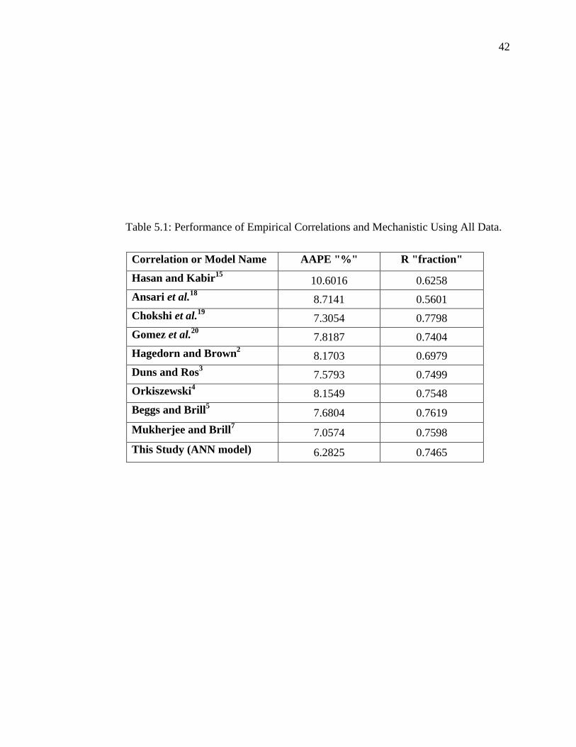
The measured (data) values of flowing bottomhole pressures were statistically
compared and cross-plotted against the predicted values. The results of this comparison
are summarized in Table 5.1. The data which consistently resulted in poor predictions by
all correlations and mechanistic models were considered to be invalid and were, therefore,
removed. A cut-off-error percentage (relative error) of 15% was implemented for the
whole data. After completion of data screening and filtering, the final number of data sets
used in developing the artificial neural network model was 206 data sets.
Partitioning the data is the process of dividing the data into three different sets:
training sets, validation sets, and test sets. By definition, the training set is used to
develop and adjust the weights in a network; the validation set is used to ensure the
generalization of the developed network during the training phase, and the test set is used
to examine the final performance of the network. The primary concerns should be to
ensure that: (a) the training set contains enough data, and suitable data distribution to
adequately cover the entire range of data, and (b) there is no unnecessary similarity
between data in different data sets. Different partitioning ratios were tested (2:1:1, 3:1:1,
and 4:1:1). The ratio of 4:1:1 (suggested by Haykin62) yielded better training and testing
results. The problem with this ratio is that it is not frequently used by researchers.
42
Table 5.1: Performance of Empirical Correlations and Mechanistic Using All Data.
Correlation or Model Name AAPE "%" R "fraction"
Hasan and Kabir15 10.6016 0.6258
Ansari et al.18 8.7141 0.5601
Chokshi et al.19 7.3054 0.7798
Gomez et al.20 7.8187 0.7404
Hagedorn and Brown2 8.1703 0.6979
Duns and Ros3 7.5793 0.7499
Orkiszewski4 8.1549 0.7548
Beggs and Brill5 7.6804 0.7619
Mukherjee and Brill7 7.0574 0.7598
This Study (ANN model) 6.2825 0.7465

43
Normally, the more training cases are submitted to the network the better
performance one can get, but the hazard of memorization becomes possible. Instead a
ratio of 3:1:1 was followed in this study. Training, validation, and testing sets are
presented in Appendix B.
5.3 Model Development 5.3.1 Introduction
Neural networks are used as computational tools with the capacity to learn, with or
without teacher, and with the ability to generalize, based on parallelism and strong
coherence between neurons in each layer. Among all types of available networks, the
most widely used are a multiple-layer feed forward networks that are capable of
representing non-linear functional mappings between inputs and outputs. The developed
model consists of one input layer (containing nine input neurons or nodes), which
represent the parameters involved in estimating bottomhole pressure (oil rate, water rate,
gas rate, diameter of the pipe, length of pipe, wellhead pressure, oil density "API", surface
temperature, and bottomhole temperature), three hidden layers (the first one contains six
nodes, the second and third hidden layer each contains three nodes) and one output layer
(contains one node) which is bottomhole pressure. This topology is achieved after a series
of optimization processes by monitoring the performance of the network until the best
network structure was accomplished.
44
5.3.2 Model Features
The developed model simply pivoted a set of processing units called neurons
equivalent to nine input variables: oil rate, water rate, gas rate, diameter of the pipe,
length of pipe, wellhead pressure, oil density "API", surface temperature, and bottomhole
temperature. In addition to these nine input parameters, one input parameter (gas specific
gravity) was discarded out because it was found insignificant.
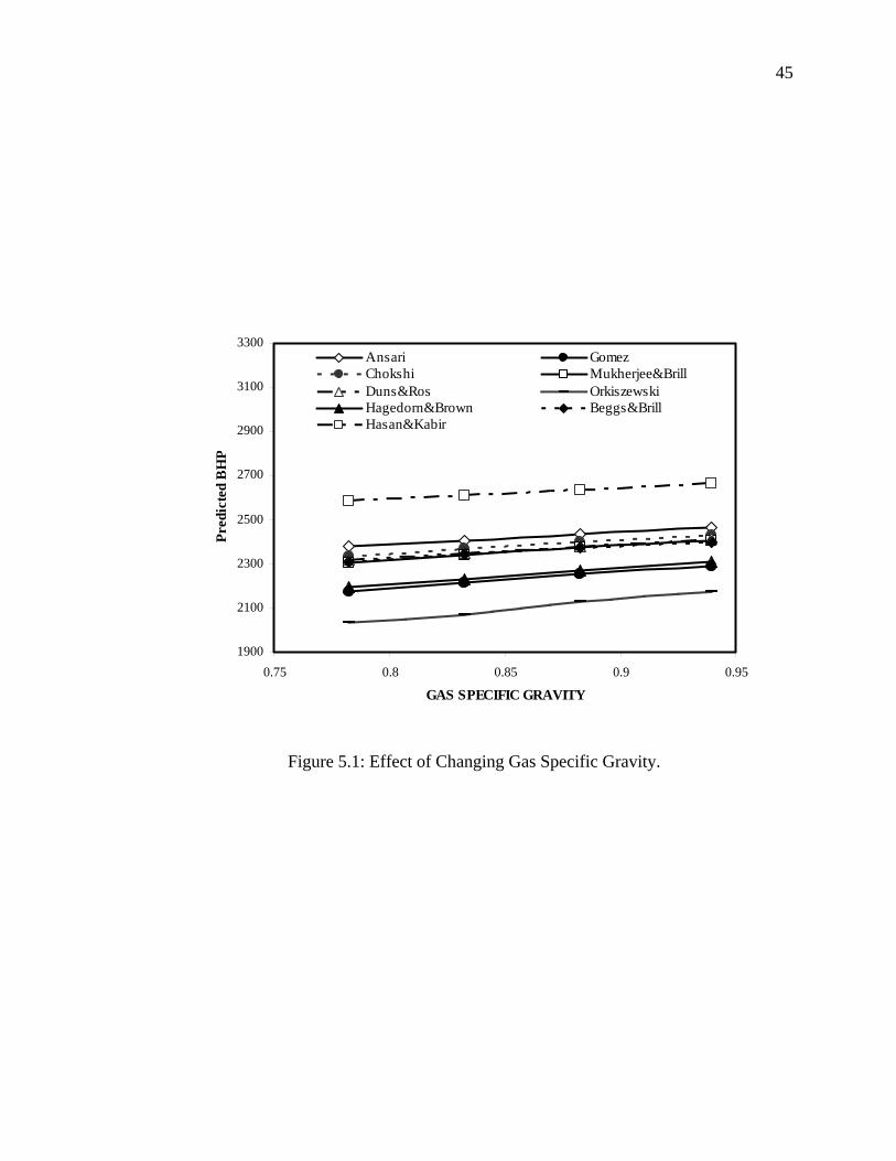
Figure 5.1 illustrates the insignificance of gas specific gravity. As shown in the
figure, predicted bottomhole pressure changes slightly for the entire range of gas specific
gravity. The model also contains an activation state for each unit, which is equivalent to
the output of the unit. Moreover, links between the units are utilized to determine the
effect of the signal of each unit. Besides, a propagation rule is used to determine the
effective input of the unit from its external inputs. An activation function (in this model
tangent hyperbolic is used for hidden units and linear for output unit), which are applied
to find out the new level of activation based on the effective input and the current
activation. Additional term was included, which is an external input bias for each hidden
layer to offer a constant offset and to minimize the number of iterations during training
process. The key feature of the model is the ability to learn from the input environment
through information gathering (learning rule).
5.3.3 Model Architecture
The number of layers, the number of processing units per layer, and the
interconnection patterns between layers defines the architecture of the model. Therefore,
45
1900
2100
2300
2500
2700
2900
3100
3300
0.75 0.8 0.85 0.9 0.95
GAS SPECIFIC GRAVITY
Pred
icte
d B
HP
Ansari GomezChokshi Mukherjee&BrillDuns&Ros OrkiszewskiHagedorn&Brown Beggs&BrillHasan&Kabir
Figure 5.1: Effect of Changing Gas Specific Gravity.
46
defining the optimal network that simulates the actual behavior within the data sets is not
an easy task. To achieve this task, certain performance criteria were followed. The design
started with small number of hidden units in the only hidden layer that it acts as a feature
detector. Some rules of thump were used as guides; for instance, the number of hidden units
should not be greater than twice the number of input variables. In addition to this rules,
several rules were suggested by different authors. Those rules can only be treated as a
rough estimation for defining hidden layers size. Those rules ignore several facts such as
the complexity and the discontinuities in the behavior under study. The basic approach
used in constructing the successful network was trial and error. The generalization error of
each inspected network design was visualized and monitored carefully through plotting the
average absolute percent error of each inspected topology. Another statistical criterion
(correlation coefficient) was utilized as a measure of tightness of estimated and measured
values to a 45 degree line. Besides, a trend analysis for each inspected model was
conducted to see whether that model simulates the real behavior. Data randomization is
necessary in constructing a successful model, while a frequently found suggestion is that
input data should describe events exhaustively; this rule of thumb can be translated into the
use of all input variables that are thought to have a problem-oriented relevance. These nine
selected input parameters were found to have pronounced effect in estimating pressure
drop.
5.3.4 Model Optimization
The optimum number of hidden units depends on many factors: the number of input
and output units, the number of training cases, the amount of noise in the targets, the
47
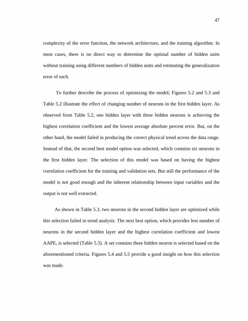
complexity of the error function, the network architecture, and the training algorithm. In
most cases, there is no direct way to determine the optimal number of hidden units
without training using different numbers of hidden units and estimating the generalization
error of each.
To further describe the process of optimizing the model; Figures 5.2 and 5.3 and
Table 5.2 illustrate the effect of changing number of neurons in the first hidden layer. As
observed from Table 5.2, one hidden layer with three hidden neurons is achieving the
highest correlation coefficient and the lowest average absolute percent error. But, on the
other hand, the model failed in producing the correct physical trend across the data range.
Instead of that, the second best model option was selected, which contains six neurons in
the first hidden layer. The selection of this model was based on having the highest
correlation coefficient for the training and validation sets. But still the performance of the
model is not good enough and the inherent relationship between input variables and the
output is not well extracted.
As shown in Table 5.3, two neurons in the second hidden layer are optimized while
this selection failed in trend analysis. The next best option, which provides less number of
neurons in the second hidden layer and the highest correlation coefficient and lowest
AAPE, is selected (Table 5.3). A set contains three hidden neuron is selected based on the
aforementioned criteria. Figures 5.4 and 5.5 provide a good insight on how this selection
was made.
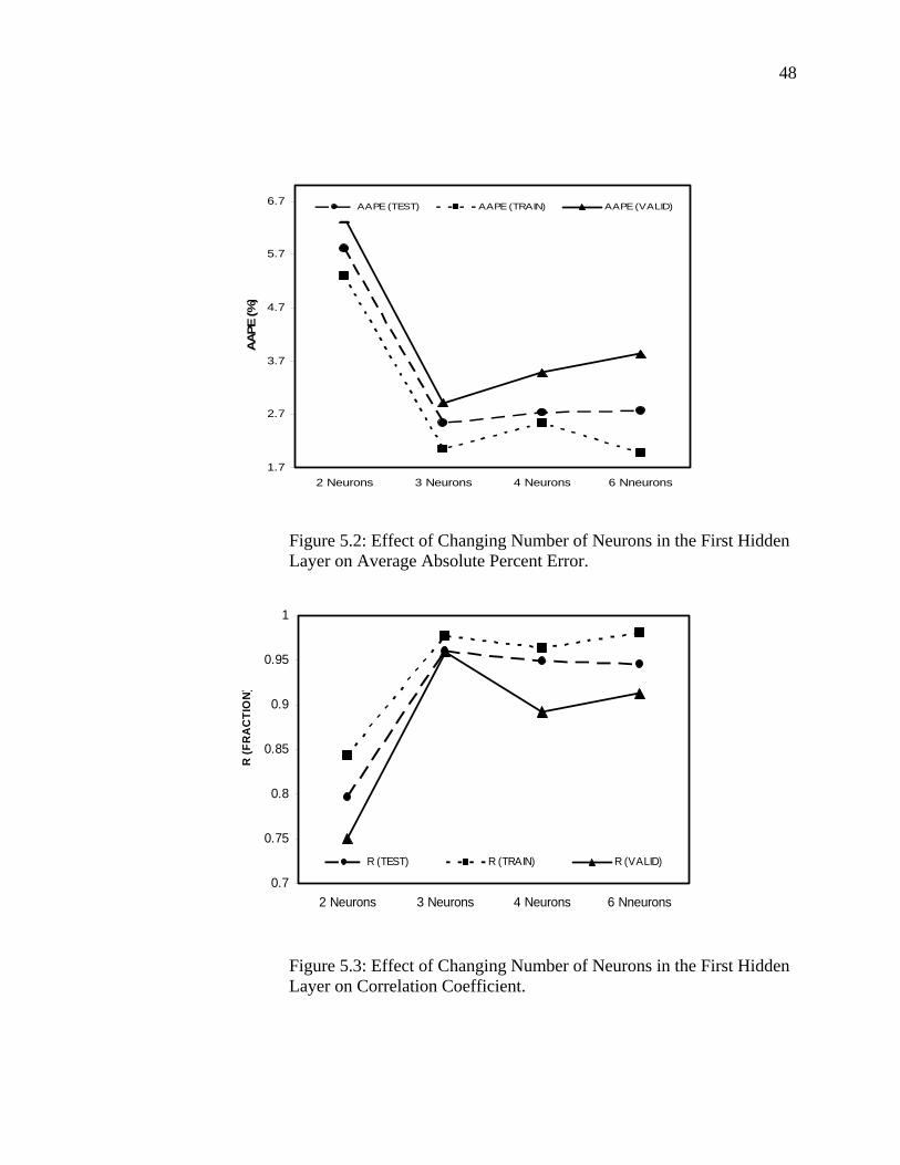
48
1.7
2.7
3.7
4.7
5.7
6.7
2 Neurons 3 Neurons 4 Neurons 6 Nneurons
AA
PE (%
)
AAPE (TEST) AAPE (TRAIN) AAPE (VALID)
Figure 5.2: Effect of Changing Number of Neurons in the First Hidden Layer on Average Absolute Percent Error.
0.7
0.75
0.8
0.85
0.9
0.95
1
2 Neurons 3 Neurons 4 Neurons 6 Nneurons
R (F
RA
CTI
ON
)
R (TEST) R (TRAIN) R (VALID)
Figure 5.3: Effect of Changing Number of Neurons in the First Hidden Layer on Correlation Coefficient.
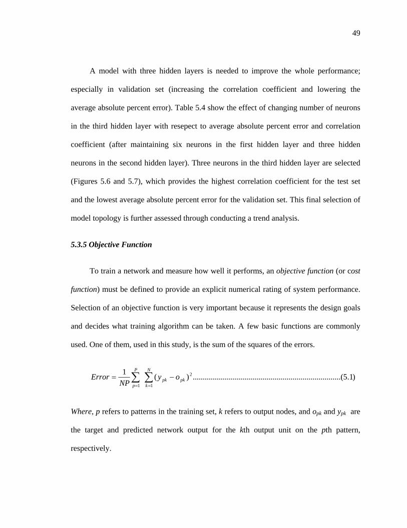
49
A model with three hidden layers is needed to improve the whole performance;
especially in validation set (increasing the correlation coefficient and lowering the
average absolute percent error). Table 5.4 show the effect of changing number of neurons
in the third hidden layer with resepect to average absolute percent error and correlation
coefficient (after maintaining six neurons in the first hidden layer and three hidden
neurons in the second hidden layer). Three neurons in the third hidden layer are selected
(Figures 5.6 and 5.7), which provides the highest correlation coefficient for the test set
and the lowest average absolute percent error for the validation set. This final selection of
model topology is further assessed through conducting a trend analysis.
5.3.5 Objective Function
To train a network and measure how well it performs, an objective function (or cost
function) must be defined to provide an explicit numerical rating of system performance.
Selection of an objective function is very important because it represents the design goals
and decides what training algorithm can be taken. A few basic functions are commonly
used. One of them, used in this study, is the sum of the squares of the errors.
)1.5....(......................................................................)(11
2
1∑∑==
−=N
kpkpk
P
poy
NPError
Where, p refers to patterns in the training set, k refers to output nodes, and opk and ypk are
the target and predicted network output for the kth output unit on the pth pattern,
respectively.

50
Table 5.2: Effect of Changing Number of Neurons in the First Hidden Layer with Resepect to Average Absolute Percent Error and Correlation Coefficient.
No of
Neurons AAPE
(TEST) AAPE
(TRAIN) AAPE
(VALID) R (TEST) R (TRAIN) R (VALID)
2 5.8079 5.2881 6.3708 0.79714 0.84343 0.75019 3 2.5378 2.048 2.9144 0.96057 0.97672 0.95937 4 2.7299 2.5421 3.4781 0.94874 0.9636 0.89206 6 2.7648 1.9733 3.8247 0.94586 0.98097 0.91255
Table 5.3: Effect of Changing Number of Neurons in the Second Hidden Layer with Resepect to Average Absolute Percent Error and Correlation Coefficient.
No of
Neurons AAPE
(TEST) AAPE
(TRAIN) AAPE
(VALID) R (TEST) R (TRAIN) R (VALID)
2 2.7576 1.2457 3.5384 0.94973 0.99167 0.92141 3 2.8539 0.61236 4.0736 0.94817 0.99749 0.90096 4 3.3088 2.2675 3.8332 0.9282 0.974 0.90242 6 3.0141 2.0547 3.5613 0.94907 0.97851 0.90973
Table 5.4: Effect of Changing Number of Neurons in the Third Hidden Layer with Resepect to Average Absolute Percent Error and Correlation Coefficient.
No of
Neurons AAPE
(TEST) AAPE
(TRAIN) AAPE
(VALID) R (TEST) R (TRAIN) R (VALID)
2 2.9799 1.5469 3.2156 0.94636 0.98593 0.94494 3 2.1598 1.7544 2.9275 0.97348 0.98461 0.93588 4 2.3929 1.9277 2.9769 0.96237 0.98072 0.95459 6 2.4878 1.1434 3.6175 0.96626 0.99265 0.91104
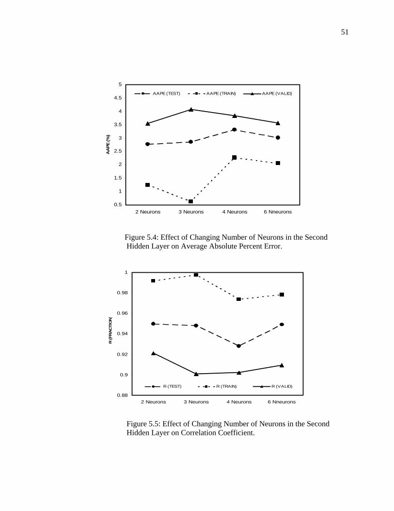
51
0.5
1
1.5
2
2.5
3
3.5
4
4.5
5
2 Neurons 3 Neurons 4 Neurons 6 Nneurons
AA
PE (%
)
AAPE (TEST) AAPE (TRAIN) AAPE (VALID)
Figure 5.4: Effect of Changing Number of Neurons in the Second Hidden Layer on Average Absolute Percent Error.
0.88
0.9
0.92
0.94
0.96
0.98
1
2 Neurons 3 Neurons 4 Neurons 6 Nneurons
R (F
RA
CTI
ON
)
R (TEST) R (TRAIN) R (VALID)
Figure 5.5: Effect of Changing Number of Neurons in the Second Hidden Layer on Correlation Coefficient.
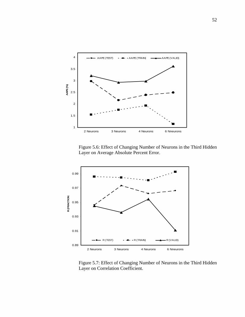
52
1
1.5
2
2.5
3
3.5
4
2 Neurons 3 Neurons 4 Neurons 6 Nneurons
AA
PE (%
)
AAPE (TEST) AAPE (TRAIN) AAPE (VALID)
Figure 5.6: Effect of Changing Number of Neurons in the Third Hidden Layer on Average Absolute Percent Error.
0.89
0.91
0.93
0.95
0.97
0.99
2 Neurons 3 Neurons 4 Neurons 6 Nneurons
R (F
RA
CTI
ON
)
R (TEST) R (TRAIN) R (VALID)
Figure 5.7: Effect of Changing Number of Neurons in the Third Hidden Layer on Correlation Coefficient.

53
5.4 Software Used
MatLab software63 (version 6.5) environment was utilized due its high range of
flexibility associated with programming and graphs visualization. Moreover, the software
offers a good way to monitor the performance of the three set of data (training, validation,
and testing) at the same time. A Matlab program is developed and training parameters
were modified in order to ensure that these parameters are well optimized. The final
model structure is shown in Figure 5.8. The problem encountered during training was the
trapping of the model in a local minima several times. The reason behind this problem
was found to be the low range of certain variables in the data. The concept of local and
global minima was discussed by several mathematicians and ANN researchers64, 65. It
defines the error gradient surface as if one look at it as a hyperbolic surface where the
global minima point lies at the bottom of this surface. Hence, beyond this point the error
starts to increase dramatically. The training session should be exactly stopped at this point
to assure the generalization of the developed model.
The default of the software is to escape only five local minima. This option has
been changed to fifteen in order to allow the network to capture the real behavior between
input parameters and output (flowing bottomhole pressure). The problem of underfitting
and overfitting (using too few; and too many units in hidden layer, respectively) was
avoided through the use of cross-validation data set. Cross-validation data set is presented
to the network after each epoch of training to check the generality (model succeeded to
capture minor relationships between input set and the desired output when new cases are
submitted to it) and stability of the model62. Input weight matrix (from input to the hidden
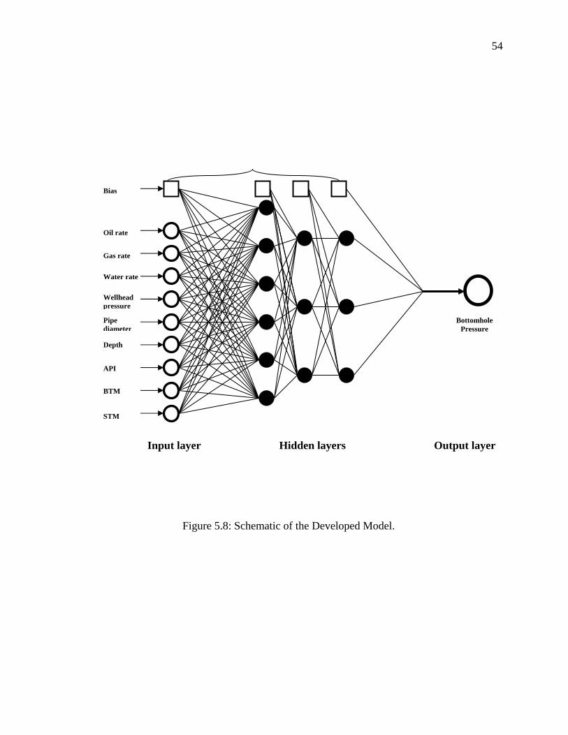
54
Figure 5.8: Schematic of the Developed Model.
Oil rate
Water rate
Gas rate
Pipe diameter
Depth
API
Wellhead pressure
BTM
STM
Bias
Output layer
BottomholePressure
Input layer Hidden layers
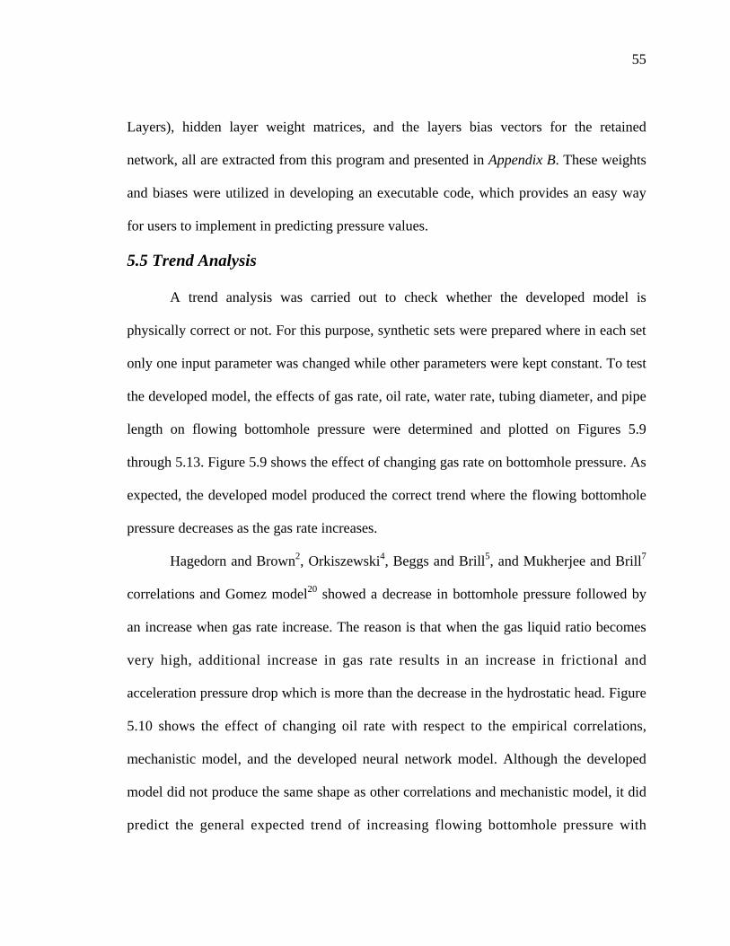
55
Layers), hidden layer weight matrices, and the layers bias vectors for the retained
network, all are extracted from this program and presented in Appendix B. These weights
and biases were utilized in developing an executable code, which provides an easy way
for users to implement in predicting pressure values.
5.5 Trend Analysis
A trend analysis was carried out to check whether the developed model is
physically correct or not. For this purpose, synthetic sets were prepared where in each set
only one input parameter was changed while other parameters were kept constant. To test
the developed model, the effects of gas rate, oil rate, water rate, tubing diameter, and pipe
length on flowing bottomhole pressure were determined and plotted on Figures 5.9
through 5.13. Figure 5.9 shows the effect of changing gas rate on bottomhole pressure. As
expected, the developed model produced the correct trend where the flowing bottomhole
pressure decreases as the gas rate increases.
Hagedorn and Brown2, Orkiszewski4, Beggs and Brill5, and Mukherjee and Brill7
correlations and Gomez model20 showed a decrease in bottomhole pressure followed by
an increase when gas rate increase. The reason is that when the gas liquid ratio becomes
very high, additional increase in gas rate results in an increase in frictional and
acceleration pressure drop which is more than the decrease in the hydrostatic head. Figure
5.10 shows the effect of changing oil rate with respect to the empirical correlations,
mechanistic model, and the developed neural network model. Although the developed
model did not produce the same shape as other correlations and mechanistic model, it did
predict the general expected trend of increasing flowing bottomhole pressure with
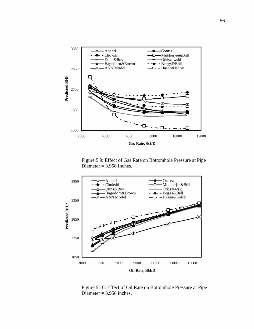
56
1350
1850
2350
2850
3350
2000 4000 6000 8000 10000 12000
Gas Rate, Scf/D
Pred
icte
d B
HP
Ansari GomezChokshi Mukherjee&BrillDuns&Ros OrkiszewskiHagedorn&Brown Beggs&BrillANN Model Hasan&Kabir
Figure 5.9: Effect of Gas Rate on Bottomhole Pressure at Pipe Diameter = 3.958 Inches.
1850
2350
2850
3350
3850
3000 5000 7000 9000 11000 13000 15000
Oil Rate, Bbl/D
Pred
icte
d B
HP
Ansari GomezChokshi Mukherjee&BrillDuns&Ros OrkiszewskiHagedorn&Brown Beggs&BrillANN Model Hasan&Kabir
Figure 5.10: Effect of Oil Rate on Bottomhole Pressure at Pipe Diameter = 3.958 inches.
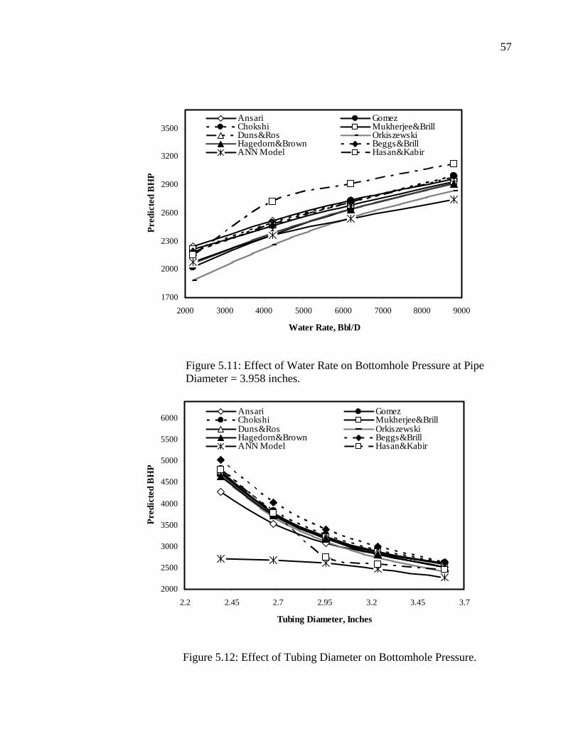
57
1700
2000
2300
2600
2900
3200
3500
2000 3000 4000 5000 6000 7000 8000 9000
Water Rate, Bbl/D
Pred
icte
d B
HP
Ansari GomezChokshi Mukherjee&BrillDuns&Ros OrkiszewskiHagedorn&Brown Beggs&BrillANN Model Hasan&Kabir
Figure 5.11: Effect of Water Rate on Bottomhole Pressure at Pipe Diameter = 3.958 inches.
2000
2500
3000
3500
4000
4500
5000
5500
6000
2.2 2.45 2.7 2.95 3.2 3.45 3.7
Tubing Diameter, Inches
Pred
icte
d B
HP
Ansari GomezChokshi Mukherjee&BrillDuns&Ros OrkiszewskiHagedorn&Brown Beggs&BrillANN Model Hasan&Kabir
Figure 5.12: Effect of Tubing Diameter on Bottomhole Pressure.
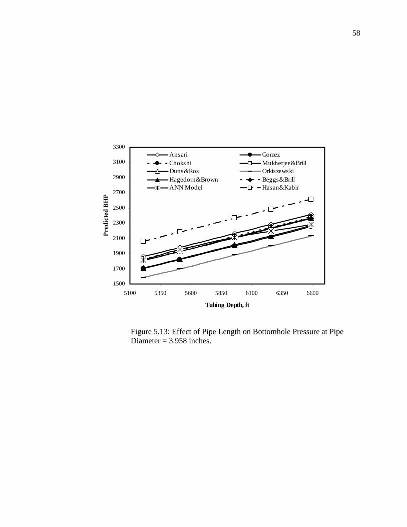
58
1500
1700
1900
2100
2300
2500
2700
2900
3100
3300
5100 5350 5600 5850 6100 6350 6600
Tubing Depth, ft
Pred
icte
d B
HP
Ansari GomezChokshi Mukherjee&BrillDuns&Ros OrkiszewskiHagedorn&Brown Beggs&BrillANN Model Hasan&Kabir
Figure 5.13: Effect of Pipe Length on Bottomhole Pressure at Pipe Diameter = 3.958 inches.
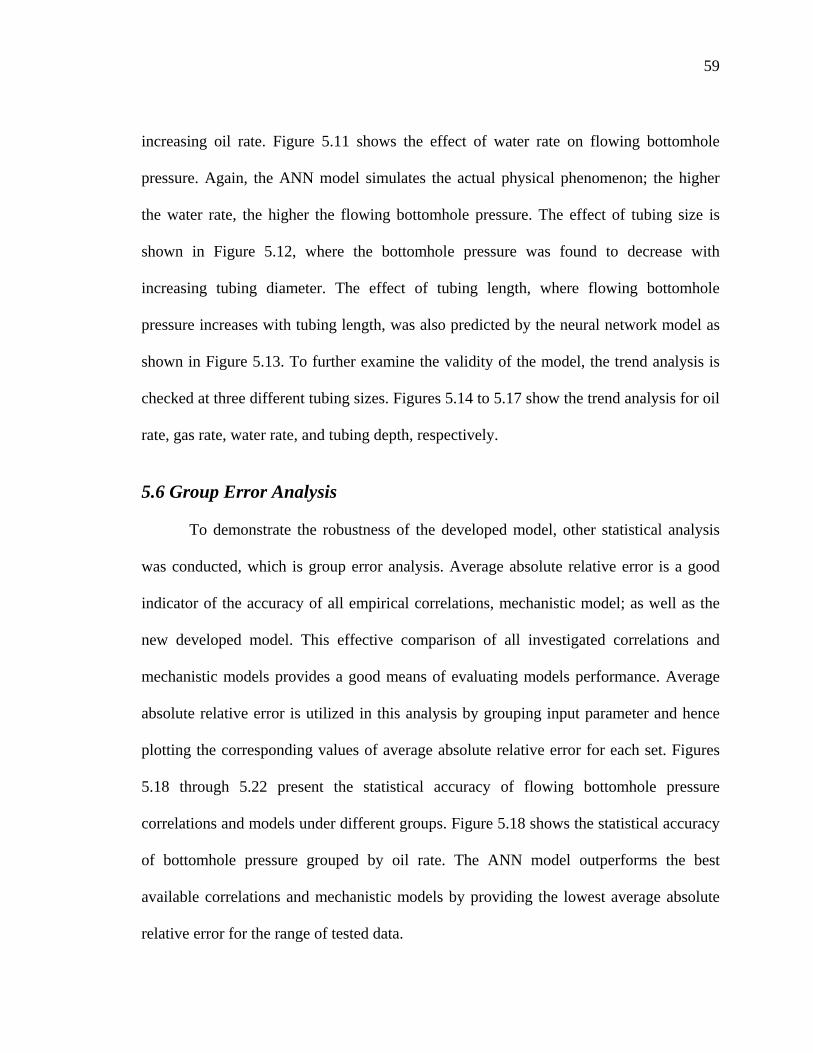
59
increasing oil rate. Figure 5.11 shows the effect of water rate on flowing bottomhole
pressure. Again, the ANN model simulates the actual physical phenomenon; the higher
the water rate, the higher the flowing bottomhole pressure. The effect of tubing size is
shown in Figure 5.12, where the bottomhole pressure was found to decrease with
increasing tubing diameter. The effect of tubing length, where flowing bottomhole
pressure increases with tubing length, was also predicted by the neural network model as
shown in Figure 5.13. To further examine the validity of the model, the trend analysis is
checked at three different tubing sizes. Figures 5.14 to 5.17 show the trend analysis for oil
rate, gas rate, water rate, and tubing depth, respectively.
5.6 Group Error Analysis
To demonstrate the robustness of the developed model, other statistical analysis
was conducted, which is group error analysis. Average absolute relative error is a good
indicator of the accuracy of all empirical correlations, mechanistic model; as well as the
new developed model. This effective comparison of all investigated correlations and
mechanistic models provides a good means of evaluating models performance. Average
absolute relative error is utilized in this analysis by grouping input parameter and hence
plotting the corresponding values of average absolute relative error for each set. Figures
5.18 through 5.22 present the statistical accuracy of flowing bottomhole pressure
correlations and models under different groups. Figure 5.18 shows the statistical accuracy
of bottomhole pressure grouped by oil rate. The ANN model outperforms the best
available correlations and mechanistic models by providing the lowest average absolute
relative error for the range of tested data.
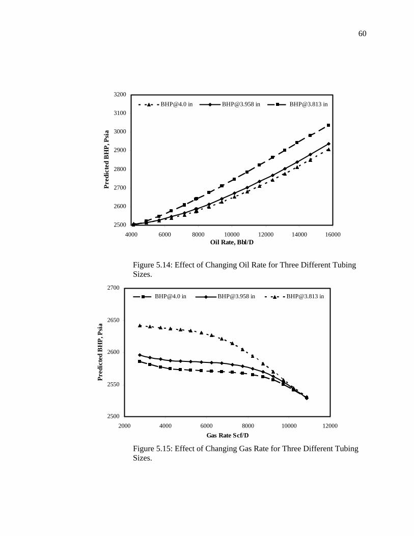
60
2500
2600
2700
2800
2900
3000
3100
3200
4000 6000 8000 10000 12000 14000 16000Oil Rate, Bbl/D
Pred
icte
d B
HP,
Psi
[email protected] in [email protected] in [email protected] in
Figure 5.14: Effect of Changing Oil Rate for Three Different Tubing Sizes.
2500
2550
2600
2650
2700
2000 4000 6000 8000 10000 12000Gas Rate Scf/D
Pred
icte
d B
HP,
Psi
a
[email protected] in [email protected] in [email protected] in
Figure 5.15: Effect of Changing Gas Rate for Three Different Tubing Sizes.
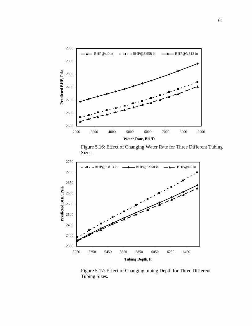
61
2600
2650
2700
2750
2800
2850
2900
2000 3000 4000 5000 6000 7000 8000 9000
Water Rate, Bbl/D
Pred
icte
d B
HP,
Psi
a
[email protected] in [email protected] in [email protected] in
Figure 5.16: Effect of Changing Water Rate for Three Different Tubing Sizes.
2350
2400
2450
2500
2550
2600
2650
2700
2750
5050 5250 5450 5650 5850 6050 6250 6450
Tubing Depth, ft
Pred
icte
d B
HP,
Psi
a
[email protected] in [email protected] in [email protected] in
Figure 5.17: Effect of Changing tubing Depth for Three Different Tubing Sizes.
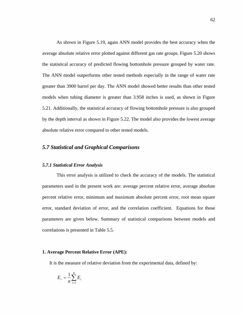
62
As shown in Figure 5.19, again ANN model provides the best accuracy when the
average absolute relative error plotted against different gas rate groups. Figure 5.20 shows
the statistical accuracy of predicted flowing bottomhole pressure grouped by water rate.
The ANN model outperforms other tested methods especially in the range of water rate
greater than 3900 barrel per day. The ANN model showed better results than other tested
models when tubing diameter is greater than 3.958 inches is used, as shown in Figure
5.21. Additionally, the statistical accuracy of flowing bottomhole pressure is also grouped
by the depth interval as shown in Figure 5.22. The model also provides the lowest average
absolute relative error compared to other tested models.
5.7 Statistical and Graphical Comparisons
5.7.1 Statistical Error Analysis
This error analysis is utilized to check the accuracy of the models. The statistical
parameters used in the present work are: average percent relative error, average absolute
percent relative error, minimum and maximum absolute percent error, root mean square
error, standard deviation of error, and the correlation coefficient. Equations for those
parameters are given below. Summary of statistical comparisons between models and
correlations is presented in Table 5.5.
1. Average Percent Relative Error (APE):
It is the measure of relative deviation from the experimental data, defined by:
∑=
=N
iir E
nE
1
1
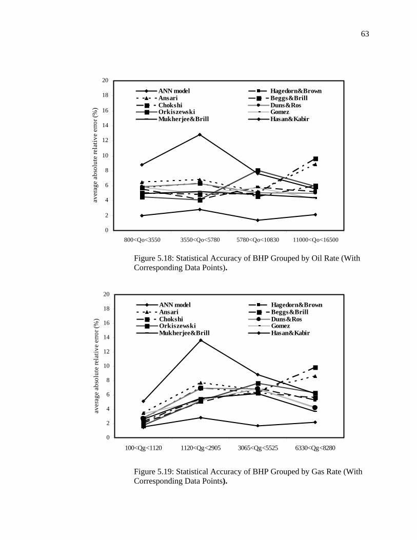
63
0
2
4
6
8
10
12
14
16
18
20
800<Qo<3550 3550<Qo<5780 5780<Qo<10830 11000<Qo<16500
aver
age
abso
lute
rela
tive
erro
r (%
)ANN model Hagedorn&BrownAnsari Beggs&BrillChokshi Duns&RosOrkiszewski GomezMukherjee&Brill Hasan&Kabir
Figure 5.18: Statistical Accuracy of BHP Grouped by Oil Rate (With Corresponding Data Points).
0
2
4
6
8
10
12
14
16
18
20
100<Qg<1120 1120<Qg<2905 3065<Qg<5525 6330<Qg<8280
aver
age
abso
lute
rela
tive
erro
r (%
)
ANN model Hagedorn&BrownAnsari Beggs&BrillChokshi Duns&RosOrkiszewski GomezMukherjee&Brill Hasan&Kabir
Figure 5.19: Statistical Accuracy of BHP Grouped by Gas Rate (With
Corresponding Data Points).
64
0
2
4
6
8
10
12
14
16
18
20
0<Qw<1015 1160<Qw<3905 4130<Qw<6500 6500<Qw<10500
aver
age
abso
lute
rela
tive
erro
r (%
)ANN model Hagedorn&BrownAnsari Beggs&BrillChokshi Duns&RosOrkiszewski GomezMukherjee&Brill Hasan&Kabir
Figure 5.20: Statistical Accuracy of BHP Grouped by Water Rate (With Corresponding Data Points).
0
2
4
6
8
10
12
14
16
18
20
Diam = 3.813 " Diam = 3.958 " Diam = 4.0 "
aver
age
abso
lute
rela
tive
erro
r (%
)
ANN model Hagedorn&BrownAnsari Beggs&BrillChokshi Duns&RosOrkiszewski GomezMukherjee&Brill Hasan&Kabir
Figure 5.21: Statistical Accuracy of BHP Grouped by Tubing Diameter (With Corresponding Data Points).
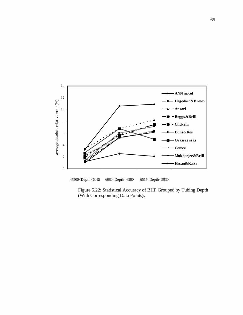
65
0
2
4
6
8
10
12
14
45500<Depth<6015 6080<Depth<6500 6515<Depth<5930
aver
age
abso
lute
rela
tive
erro
r (%
)
ANN model
Hagedorn&Brown
Ansari
Beggs&Brill
Chokshi
Duns&Ros
Orkiszewski
Gomez
Mukherjee&Brill
Hasan&Kabir
Figure 5.22: Statistical Accuracy of BHP Grouped by Tubing Depth (With Corresponding Data Points).
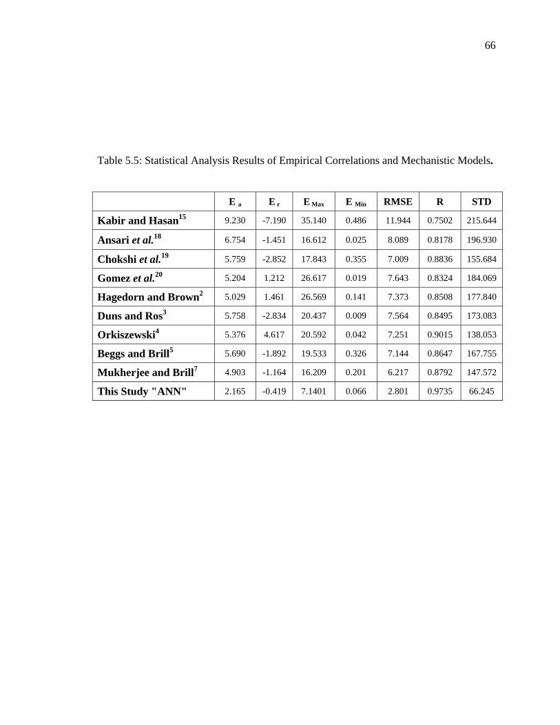
66
Table 5.5: Statistical Analysis Results of Empirical Correlations and Mechanistic Models.
E a E r E Max E Min RMSE R STD
Kabir and Hasan15 9.230 -7.190 35.140 0.486 11.944 0.7502 215.644
Ansari et al.18 6.754 -1.451 16.612 0.025 8.089 0.8178 196.930
Chokshi et al.19 5.759 -2.852 17.843 0.355 7.009 0.8836 155.684
Gomez et al.20 5.204 1.212 26.617 0.019 7.643 0.8324 184.069
Hagedorn and Brown2 5.029 1.461 26.569 0.141 7.373 0.8508 177.840
Duns and Ros3 5.758 -2.834 20.437 0.009 7.564 0.8495 173.083
Orkiszewski4 5.376 4.617 20.592 0.042 7.251 0.9015 138.053
Beggs and Brill5 5.690 -1.892 19.533 0.326 7.144 0.8647 167.755
Mukherjee and Brill7 4.903 -1.164 16.209 0.201 6.217 0.8792 147.572
This Study "ANN" 2.165 -0.419 7.1401 0.066 2.801 0.9735 66.245
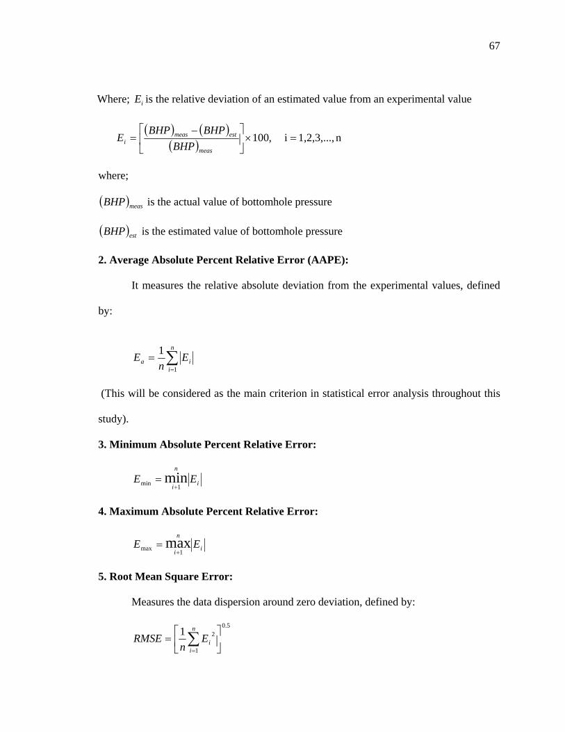
67
Where; iE is the relative deviation of an estimated value from an experimental value
( ) ( )( ) n1,2,3,...,i ,100 =×⎥
⎦
⎤⎢⎣
⎡ −=
meas
estmeasi BHP
BHPBHPE
where;
( )measBHP is the actual value of bottomhole pressure
( )estBHP is the estimated value of bottomhole pressure
2. Average Absolute Percent Relative Error (AAPE):
It measures the relative absolute deviation from the experimental values, defined
by:
∑=
=n
iia E
nE
1
1
(This will be considered as the main criterion in statistical error analysis throughout this
study).
3. Minimum Absolute Percent Relative Error:
i
n
iEE
1min min+
=
4. Maximum Absolute Percent Relative Error:
i
n
iEE
1max max+
=
5. Root Mean Square Error:
Measures the data dispersion around zero deviation, defined by:
5.0
1
21⎥⎦
⎤⎢⎣
⎡= ∑
=
n
iiE
nRMSE
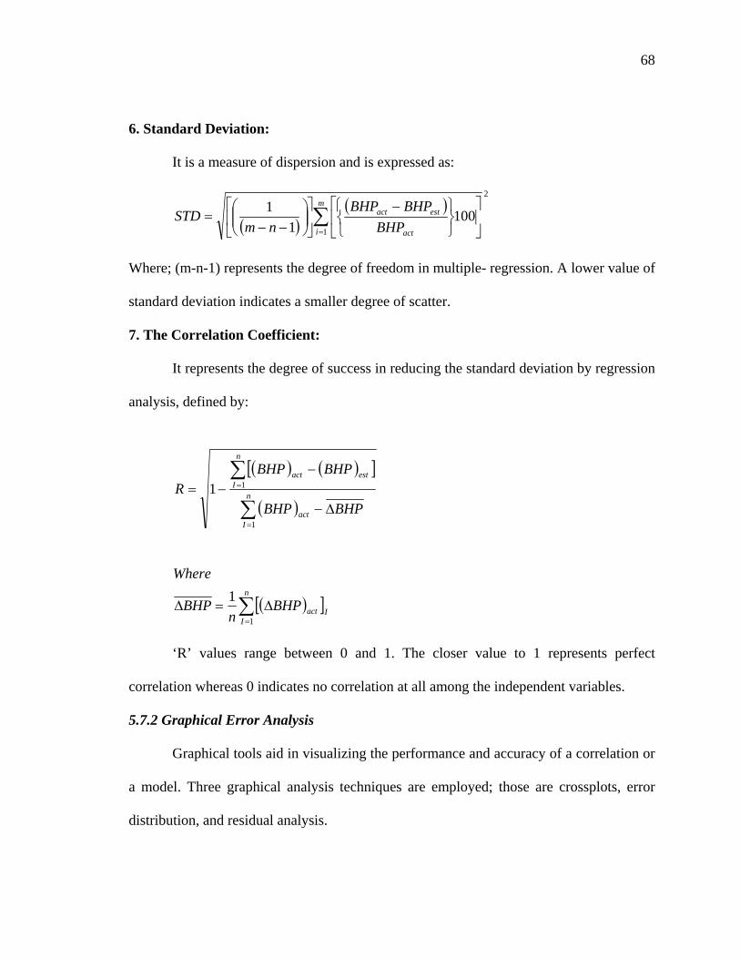
68
6. Standard Deviation:
It is a measure of dispersion and is expressed as:
( )( )
2
1100
11 ∑
=⎥⎦
⎤⎢⎣
⎡
⎭⎬⎫
⎩⎨⎧ −
⎥⎦
⎤⎢⎣
⎡⎟⎟⎠
⎞⎜⎜⎝
⎛−−
=m
i act
estact
BHPBHPBHP
nmSTD
Where; (m-n-1) represents the degree of freedom in multiple- regression. A lower value of
standard deviation indicates a smaller degree of scatter.
7. The Correlation Coefficient:
It represents the degree of success in reducing the standard deviation by regression
analysis, defined by:
( )[ ]∑=
∆=∆n
IIactBHP
nBHP
Where
1
1
‘R’ values range between 0 and 1. The closer value to 1 represents perfect
correlation whereas 0 indicates no correlation at all among the independent variables.
5.7.2 Graphical Error Analysis
Graphical tools aid in visualizing the performance and accuracy of a correlation or
a model. Three graphical analysis techniques are employed; those are crossplots, error
distribution, and residual analysis.
( ) ( )[ ]
( )∑
∑
=
=
∆−
−−= n
Iact
n
Iestact
BHPBHP
BHPBHPR
1
11
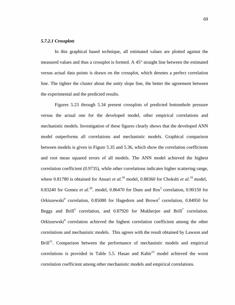
69
5.7.2.1 Crossplots
In this graphical based technique, all estimated values are plotted against the
measured values and thus a crossplot is formed. A 45° straight line between the estimated
versus actual data points is drawn on the crossplot, which denotes a perfect correlation
line. The tighter the cluster about the unity slope line, the better the agreement between
the experimental and the predicted results.
Figures 5.23 through 5.34 present crossplots of predicted bottomhole pressure
versus the actual one for the developed model, other empirical correlations and
mechanistic models. Investigation of these figures clearly shows that the developed ANN
model outperforms all correlations and mechanistic models. Graphical comparison
between models is given in Figure 5.35 and 5.36, which show the correlation coefficients
and root mean squared errors of all models. The ANN model achieved the highest
correlation coefficient (0.9735), while other correlations indicates higher scattering range,
where 0.81780 is obtained for Ansari et al.18 model, 0.88360 for Chokshi et al.19 model,
0.83240 for Gomez et al.20. model, 0.86470 for Duns and Ros3 correlation, 0.90150 for
Orkiszewski4 correlation, 0.85080 for Hagedorn and Brown2 correlation, 0.84950 for
Beggs and Brill5 correlation, and 0.87920 for Mukherjee and Brill7 correlation.
Orkiszewski4 correlation achieved the highest correlation coefficient among the other
correlations and mechanistic models. This agrees with the result obtained by Lawson and
Brill11. Comparison between the performance of mechanistic models and empirical
correlations is provided in Table 5.5. Hasan and Kabir15 model achieved the worst
correlation coefficient among other mechanistic models and empirical correlations.
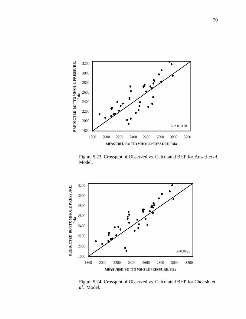
70
1800
2000
2200
2400
2600
2800
3000
3200
1800 2000 2200 2400 2600 2800 3000 3200
MEASURED BO TTO MHOLE PRESSURE, Psia
PRED
ICTE
D B
OTT
OM
HO
LE P
RES
SUR
E,
Psia
R = 0.8178
Figure 5.23: Crossplot of Observed vs. Calculated BHP for Ansari et al.
Model.
1800
2000
2200
2400
2600
2800
3000
3200
1800 2000 2200 2400 2600 2800 3000 3200
MEASURED BO TTO MHO LE PRESSURE, Psia
PRED
ICTE
D B
OTT
OM
HO
LE P
RES
SUR
E,
Psia
R=0.8836
Figure 5.24: Crossplot of Observed vs. Calculated BHP for Chokshi et
al. Model.
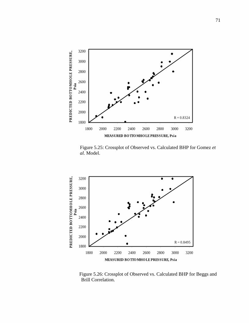
71
1800
2000
2200
2400
2600
2800
3000
3200
1800 2000 2200 2400 2600 2800 3000 3200
MEASURED BO TTO MHO LE PRESSURE, Psia
PRED
ICTE
D B
OTT
OM
HO
LE P
RES
SUR
E,
Psia
R = 0.8324
Figure 5.25: Crossplot of Observed vs. Calculated BHP for Gomez et
al. Model.
1800
2000
2200
2400
2600
2800
3000
3200
1800 2000 2200 2400 2600 2800 3000 3200
MEASURED BO TTO MHO LE PRESSURE, Psia
PRED
ICTE
D B
OTT
OM
HO
LE P
RES
SUR
E,
Psia
R = 0.8495
Figure 5.26: Crossplot of Observed vs. Calculated BHP for Beggs and
Brill Correlation.
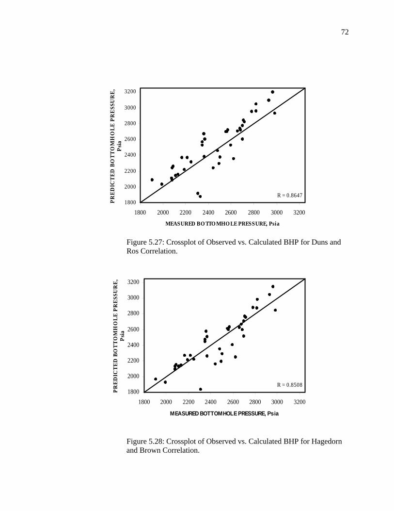
72
1800
2000
2200
2400
2600
2800
3000
3200
1800 2000 2200 2400 2600 2800 3000 3200
MEASURED BO TTO MHO LE PRESSURE, Psia
PRED
ICTE
D B
OTT
OM
HO
LE P
RES
SUR
E,
Psia
R = 0.8647
Figure 5.27: Crossplot of Observed vs. Calculated BHP for Duns and
Ros Correlation.
1800
2000
2200
2400
2600
2800
3000
3200
1800 2000 2200 2400 2600 2800 3000 3200
MEASURED BOTTOMHOLE PRESSURE, Psia
PRED
ICTE
D B
OTT
OM
HO
LE P
RES
SUR
E,
Psia
R = 0.8508
Figure 5.28: Crossplot of Observed vs. Calculated BHP for Hagedorn and Brown Correlation.
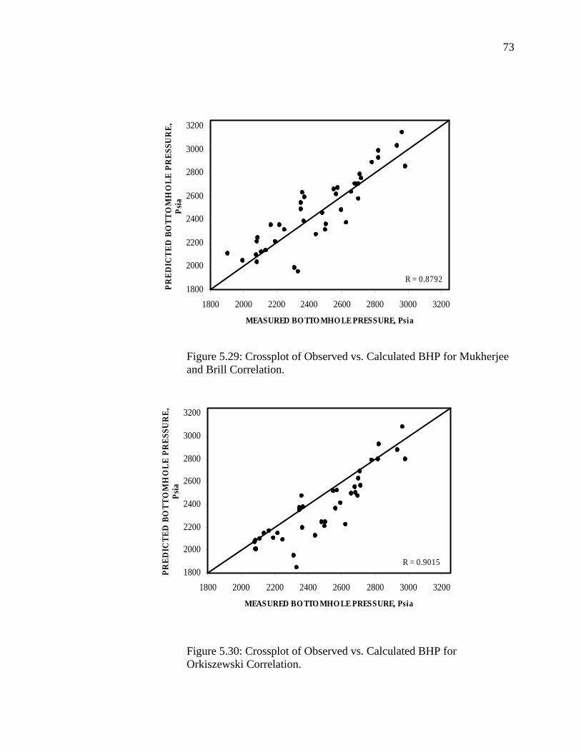
73
1800
2000
2200
2400
2600
2800
3000
3200
1800 2000 2200 2400 2600 2800 3000 3200
MEASURED BO TTO MHO LE PRESSURE, Psia
PRED
ICTE
D B
OTT
OM
HO
LE P
RES
SUR
E,
Psia
R = 0.8792
Figure 5.29: Crossplot of Observed vs. Calculated BHP for Mukherjee
and Brill Correlation.
1800
2000
2200
2400
2600
2800
3000
3200
1800 2000 2200 2400 2600 2800 3000 3200
MEASURED BO TTO MHO LE PRESSURE, Psia
PRED
ICTE
D B
OTT
OM
HO
LE P
RES
SUR
E,
Psia
R = 0.9015
Figure 5.30: Crossplot of Observed vs. Calculated BHP for Orkiszewski Correlation.
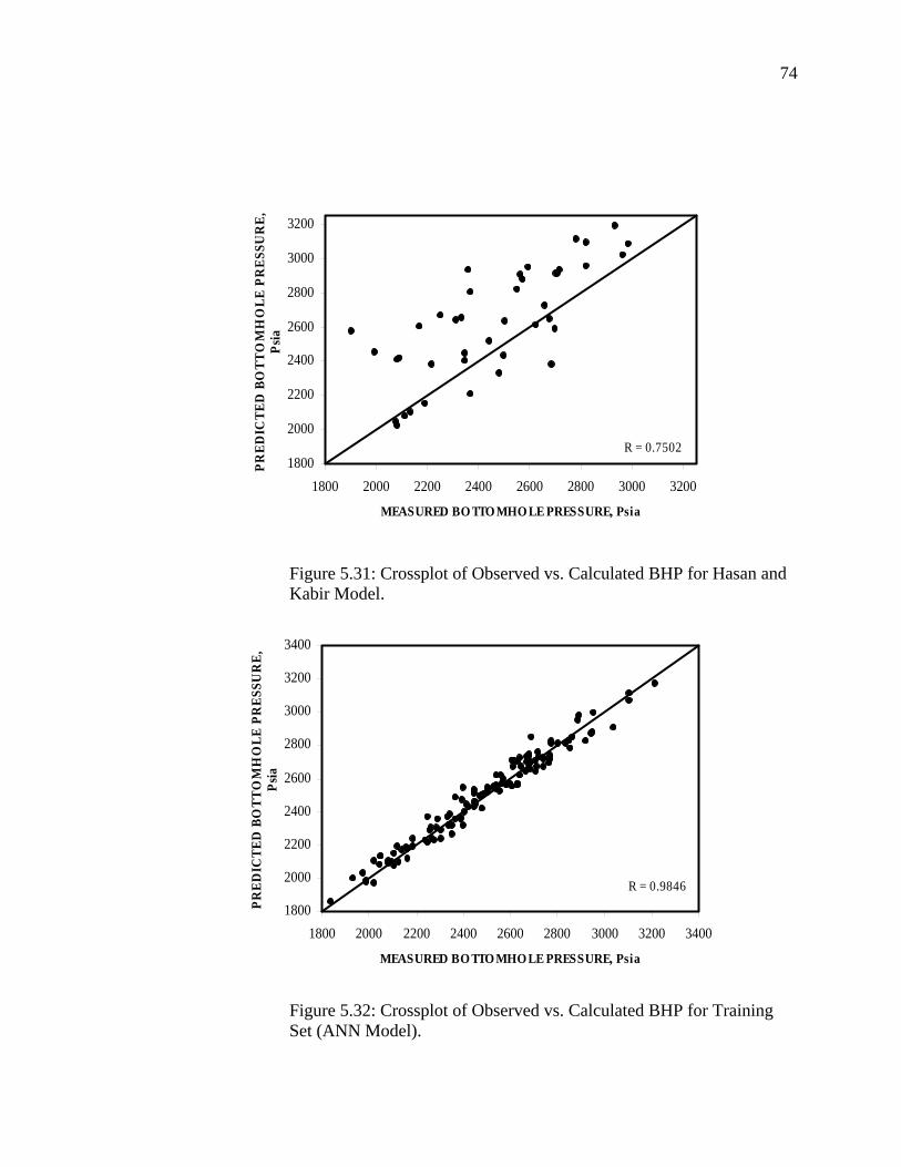
74
1800
2000
2200
2400
2600
2800
3000
3200
1800 2000 2200 2400 2600 2800 3000 3200
MEASURED BO TTO MHO LE PRESSURE, Psia
PRED
ICTE
D B
OTT
OM
HO
LE P
RES
SUR
E,
Psia
R = 0.7502
Figure 5.31: Crossplot of Observed vs. Calculated BHP for Hasan and Kabir Model.
1800
2000
2200
2400
2600
2800
3000
3200
3400
1800 2000 2200 2400 2600 2800 3000 3200 3400
MEASURED BO TTO MHO LE PRESSURE, Psia
PRED
ICTE
D B
OTT
OM
HO
LE P
RES
SUR
E,
Psia
R = 0.9846
Figure 5.32: Crossplot of Observed vs. Calculated BHP for Training
Set (ANN Model).
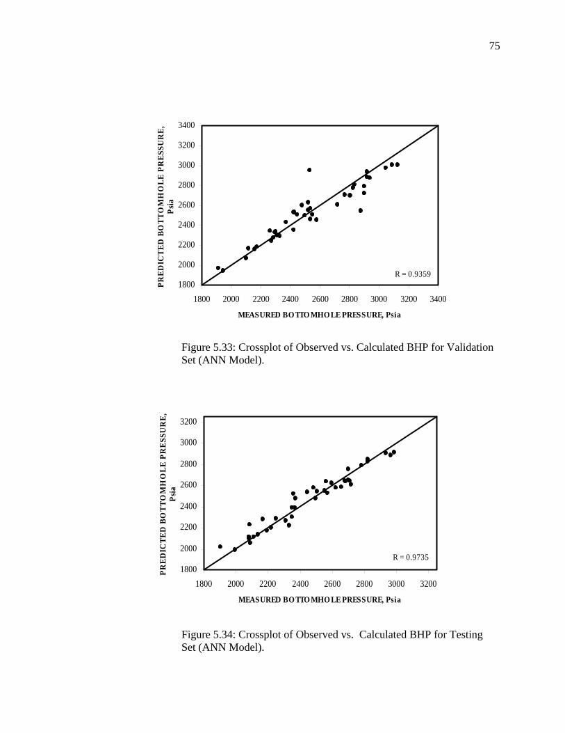
75
1800
2000
2200
2400
2600
2800
3000
3200
3400
1800 2000 2200 2400 2600 2800 3000 3200 3400
MEASURED BO TTO MHO LE PRESSURE, Psia
PRED
ICTE
D B
OTT
OM
HO
LE P
RES
SUR
E,
Psia
R = 0.9359
Figure 5.33: Crossplot of Observed vs. Calculated BHP for Validation
Set (ANN Model).
1800
2000
2200
2400
2600
2800
3000
3200
1800 2000 2200 2400 2600 2800 3000 3200
MEASURED BO TTO MHO LE PRESSURE, Psia
PRED
ICTE
D B
OTT
OM
HO
LE P
RES
SUR
E,
Psia
R = 0.9735
Figure 5.34: Crossplot of Observed vs. Calculated BHP for Testing
Set (ANN Model).
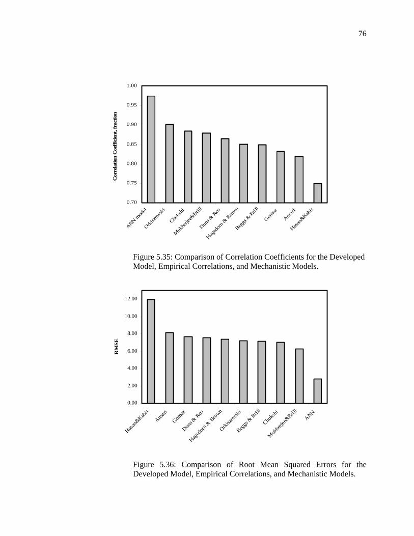
76
0.70
0.75
0.80
0.85
0.90
0.95
1.00
ANN mod
el
Orkisze
wski
Choks
hi
Muk
herje
e&Bril
l
Duns &
Ros
Haged
orn &
Brow
n
Beggs
& B
rill
Gomez
Ansari
Hasan&
Kabir
Cor
rela
tion
Coe
ffic
ient
, fra
ctio
n
Figure 5.35: Comparison of Correlation Coefficients for the Developed
Model, Empirical Correlations, and Mechanistic Models.
0.00
2.00
4.00
6.00
8.00
10.00
12.00
Hasan&
Kabir
Ansari
Gomez
Duns &
Ros
Haged
orn &
Brow
n
Orkisze
wski
Beggs
& B
rill
Choks
hi
Muk
herje
e&Bril
lANN
RM
SE
Figure 5.36: Comparison of Root Mean Squared Errors for the Developed Model, Empirical Correlations, and Mechanistic Models.
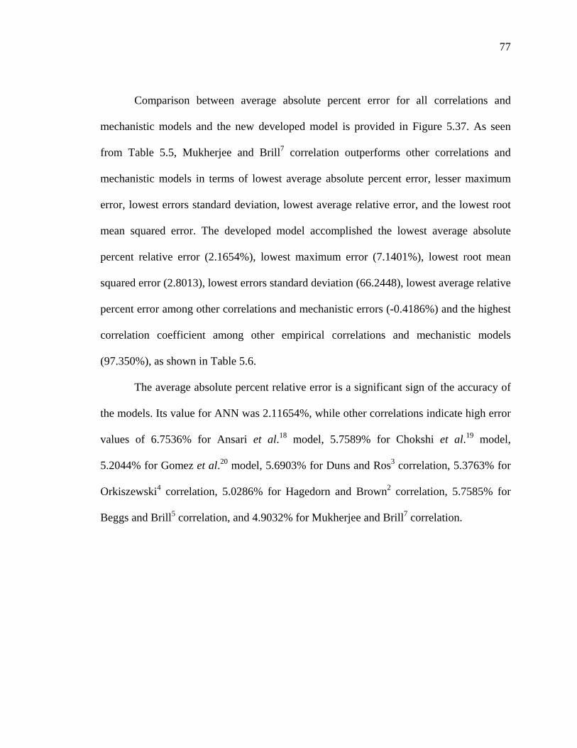
77
Comparison between average absolute percent error for all correlations and
mechanistic models and the new developed model is provided in Figure 5.37. As seen
from Table 5.5, Mukherjee and Brill7 correlation outperforms other correlations and
mechanistic models in terms of lowest average absolute percent error, lesser maximum
error, lowest errors standard deviation, lowest average relative error, and the lowest root
mean squared error. The developed model accomplished the lowest average absolute
percent relative error (2.1654%), lowest maximum error (7.1401%), lowest root mean
squared error (2.8013), lowest errors standard deviation (66.2448), lowest average relative
percent error among other correlations and mechanistic errors (-0.4186%) and the highest
correlation coefficient among other empirical correlations and mechanistic models
(97.350%), as shown in Table 5.6.
The average absolute percent relative error is a significant sign of the accuracy of
the models. Its value for ANN was 2.11654%, while other correlations indicate high error
values of 6.7536% for Ansari et al.18 model, 5.7589% for Chokshi et al.19 model,
5.2044% for Gomez et al.20 model, 5.6903% for Duns and Ros3 correlation, 5.3763% for
Orkiszewski4 correlation, 5.0286% for Hagedorn and Brown2 correlation, 5.7585% for
Beggs and Brill5 correlation, and 4.9032% for Mukherjee and Brill7 correlation.
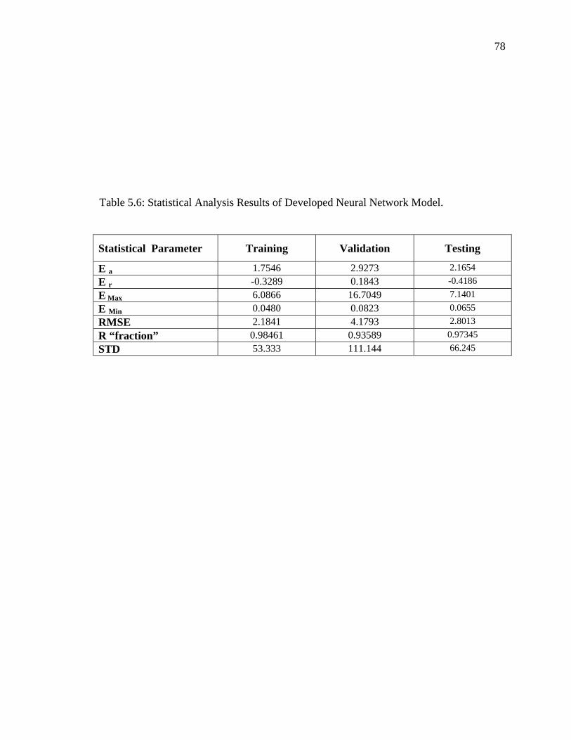
78
Table 5.6: Statistical Analysis Results of Developed Neural Network Model.
Statistical Parameter Training Validation Testing
E a 1.7546 2.9273 2.1654 E r -0.3289 0.1843 -0.4186 E Max 6.0866 16.7049 7.1401 E Min 0.0480 0.0823 0.0655 RMSE 2.1841 4.1793 2.8013 R “fraction” 0.98461 0.93589 0.97345 STD 53.333 111.144 66.245

79
5.7.2.2 Error Distributions
Figures 5.38 through 5.40 show the error distribution histograms for the neural
network model. Normal distribution curves are fitted to each one of them. The errors are
said to be normally distributed with a mean around the 0%. Hence, most investigated
correlations and mechanistic models show either slight negatively skewed error
distributed or positively ones.
Figure 5.41 shows the error distribution histogram and the normal distribution
curve for Ansari et al.18 model. It shows a slight shift of the mean of the errors towards
the negative side of the plot (about two degrees) indicating that the flowing bottomhole
pressure is overestimated. Figure 5.42 shows the error distribution histogram and the
normal distribution curve for Chokshi et al.19 model. The errors are normally distributed
with a mean approximately equals to -3%, indicating the model is overestimating the
flowing bottomhole pressure. Figure 5.43 shows the error distribution histogram and the
normal distribution curve for Gomez et al.20 model. The model shows good performance
with reasonable error distributed (shifted 0.5% to the positive side). Figure 5.44 shows the
error distribution histogram and the normal distribution curve for Beggs and Brill5
correlation. The correlation errors histogram suffered from a pronounced shift towards the
left (-3%), indicating that correlation overpredicted the flowing bottomhole pressure.
Figure 5.45 shows the error distribution histogram and the normal distribution curve for
Duns and Ros3 correlation. The correlation overestimates the pressure due to the shift of
its normal distribution curve towards the left (-2%). On contradictory, Hagedorn and
Brown2 correlation underestimates the pressure (Figure 5.46) due to the shift of the
normal distribution curve to the right side (1.5%). It is evident that, from Mukherjee and
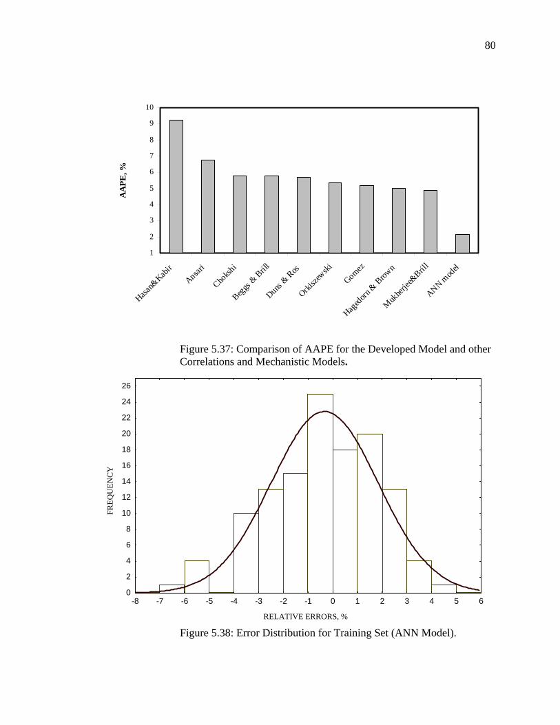
80
1
2
3
4
5
6
7
8
9
10
Hasan&
Kabir
Ansari
Choksh
i
Beggs & Brill
Duns & Ros
Orkisze
wski
Gomez
Hagedorn
& Brow
n
Mukher
jee&Brill
ANN mod
el
AA
PE, %
Figure 5.37: Comparison of AAPE for the Developed Model and other Correlations and Mechanistic Models.
RELATIVE ERRORS, %
FREQ
UEN
CY
0
2
4
6
8
10
12
14
16
18
20
22
24
26
-8 -7 -6 -5 -4 -3 -2 -1 0 1 2 3 4 5 6
Figure 5.38: Error Distribution for Training Set (ANN Model).
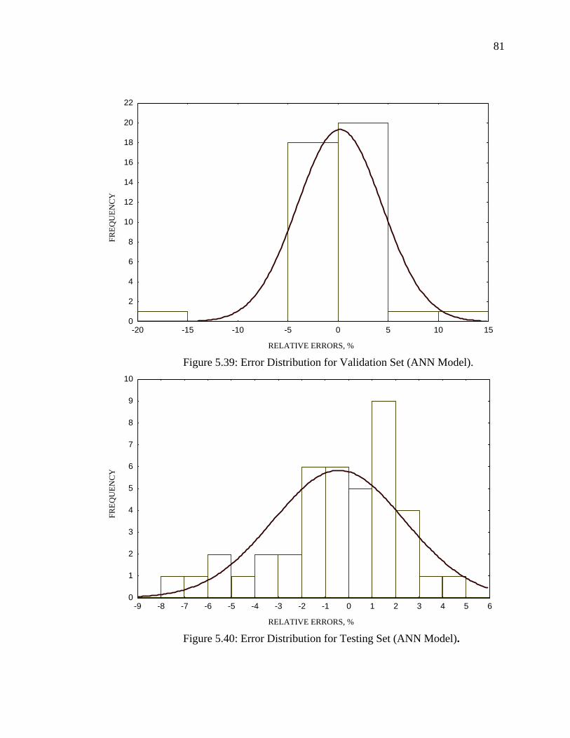
81
RELATIVE ERRORS, %
FREQ
UEN
CY
0
2
4
6
8
10
12
14
16
18
20
22
-20 -15 -10 -5 0 5 10 15
Figure 5.39: Error Distribution for Validation Set (ANN Model).
RELATIVE ERRORS, %
FREQ
UEN
CY
0
1
2
3
4
5
6
7
8
9
10
-9 -8 -7 -6 -5 -4 -3 -2 -1 0 1 2 3 4 5 6
Figure 5.40: Error Distribution for Testing Set (ANN Model).
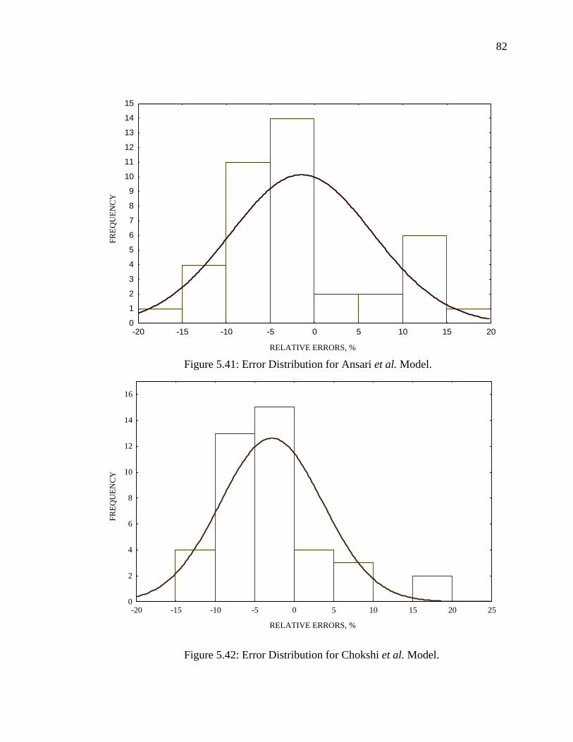
82
RELATIVE ERRORS, %
FREQ
UEN
CY
0
1
2
3
4
5
6
7
8
9
10
11
12
13
14
15
-20 -15 -10 -5 0 5 10 15 20
Figure 5.41: Error Distribution for Ansari et al. Model.
RELATIVE ERRORS, %
FREQ
UEN
CY
0
2
4
6
8
10
12
14
16
-20 -15 -10 -5 0 5 10 15 20 25
Figure 5.42: Error Distribution for Chokshi et al. Model.
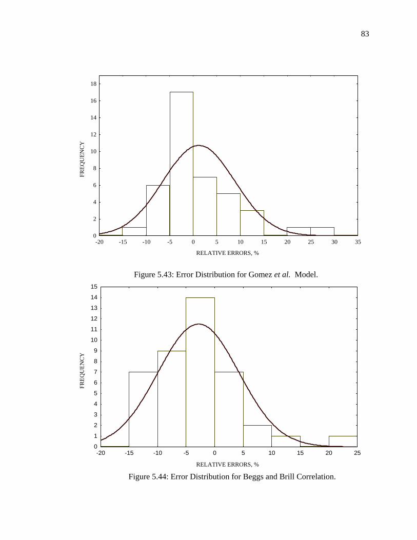
83
RELATIVE ERRORS, %
FREQ
UEN
CY
0
2
4
6
8
10
12
14
16
18
-20 -15 -10 -5 0 5 10 15 20 25 30 35
Figure 5.43: Error Distribution for Gomez et al. Model.
RELATIVE ERRORS, %
FREQ
UEN
CY
0
1
2
3
4
5
6
7
8
9
10
11
12
13
14
15
-20 -15 -10 -5 0 5 10 15 20 25
Figure 5.44: Error Distribution for Beggs and Brill Correlation.
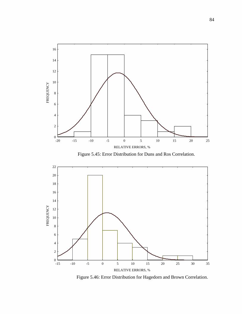
84
RELATIVE ERRORS, %
FREQ
UEN
CY
0
2
4
6
8
10
12
14
16
-20 -15 -10 -5 0 5 10 15 20 25
Figure 5.45: Error Distribution for Duns and Ros Correlation.
RELATIVE ERRORS, %
FREQ
UEN
CY
0
2
4
6
8
10
12
14
16
18
20
22
-15 -10 -5 0 5 10 15 20 25 30 35
Figure 5.46: Error Distribution for Hagedorn and Brown Correlation.
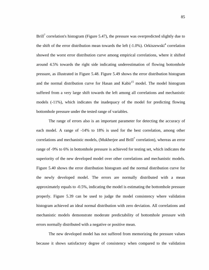
85
Brill7 correlation's histogram (Figure 5.47), the pressure was overpredicted slightly due to
the shift of the error distribution mean towards the left (-1.0%). Orkiszewski4 correlation
showed the worst error distribution curve among empirical correlations, where it shifted
around 4.5% towards the right side indicating underestimation of flowing bottomhole
pressure, as illustrated in Figure 5.48. Figure 5.49 shows the error distribution histogram
and the normal distribution curve for Hasan and Kabir15 model. The model histogram
suffered from a very large shift towards the left among all correlations and mechanistic
models (-11%), which indicates the inadequacy of the model for predicting flowing
bottomhole pressure under the tested range of variables.
The range of errors also is an important parameter for detecting the accuracy of
each model. A range of -14% to 18% is used for the best correlation, among other
correlations and mechanistic models, (Mukherjee and Brill7 correlation), whereas an error
range of -9% to 6% in bottomhole pressure is achieved for testing set, which indicates the
superiority of the new developed model over other correlations and mechanistic models.
Figure 5.40 shows the error distribution histogram and the normal distribution curve for
the newly developed model. The errors are normally distributed with a mean
approximately equals to -0.5%, indicating the model is estimating the bottomhole pressure
properly. Figure 5.39 can be used to judge the model consistency where validation
histogram achieved an ideal normal distribution with zero deviation. All correlations and
mechanistic models demonstrate moderate predictability of bottomhole pressure with
errors normally distributed with a negative or positive mean.
The new developed model has not suffered from memorizing the pressure values
because it shows satisfactory degree of consistency when compared to the validation

86
results. If the correlation coefficient is used as a main criterion for selecting the best
overall performance, Orkiszewski4 correlation could be selected based on this feature.
Because standard deviation is one of the measures of scattering tendencies, it is included
as a measure of how points are distributed and scattered. Based on this criterion,
Orkiszewski4 correlation performs the best (138.053) followed by Mukherjee and Brill7
correlation (147.572) and Chokshi et al.19 model (155.684).
Mukherjee and Brill7 correlation showed the lowest average absolute percent
error, the lowest RMSE, the lowest maximum error, the lowest average relative percent
error, and the second best in standard deviation measurement compared to the other
correlations and mechanistic models. Moreover, it is noted that at reasonably low gas-
liquid ratios and gas-oil ratios, Mukherjee and Brill7 correlation performs the best when
compared to the rest of correlations and mechanistic models.
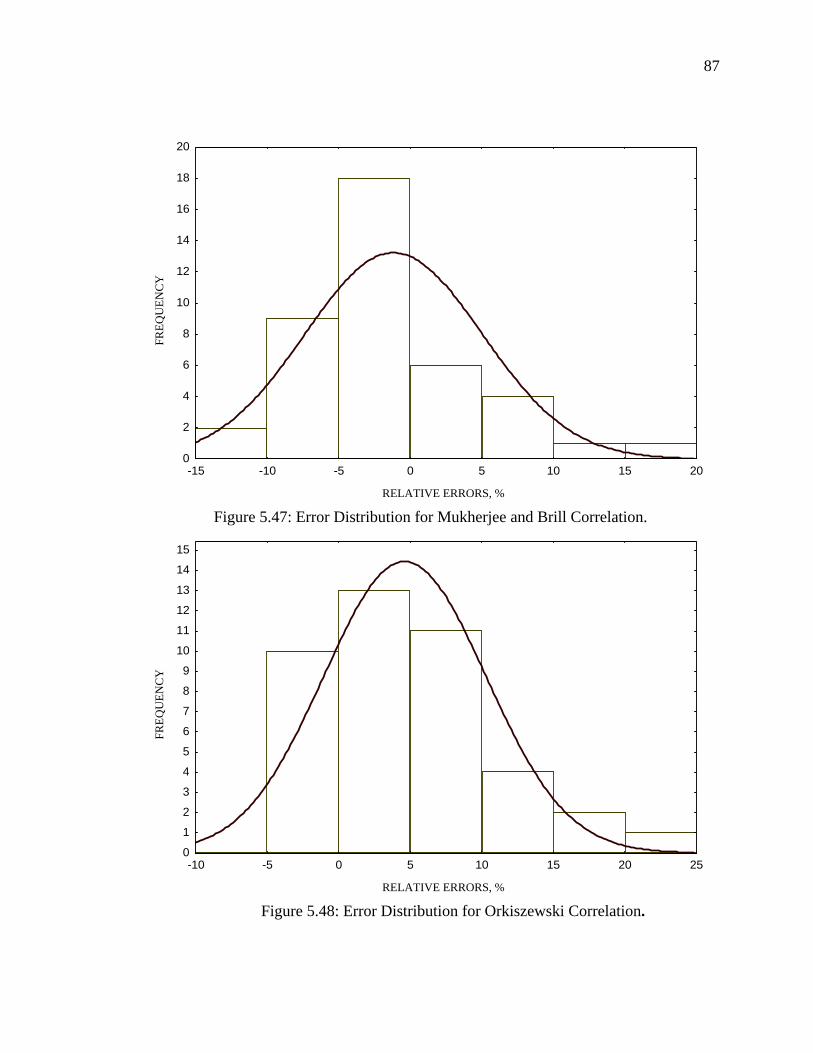
87
RELATIVE ERRORS, %
FREQ
UEN
CY
0
2
4
6
8
10
12
14
16
18
20
-15 -10 -5 0 5 10 15 20
Figure 5.47: Error Distribution for Mukherjee and Brill Correlation.
RELATIVE ERRORS, %
FREQ
UEN
CY
0
1
2
3
4
5
6
7
8
9
10
11
12
13
14
15
-10 -5 0 5 10 15 20 25
Figure 5.48: Error Distribution for Orkiszewski Correlation.
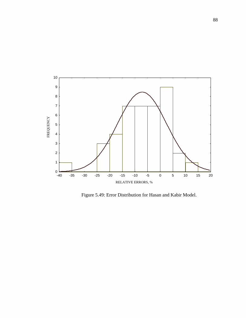
88
RELATIVE ERRORS, %
FREQ
UEN
CY
0
1
2
3
4
5
6
7
8
9
10
-40 -35 -30 -25 -20 -15 -10 -5 0 5 10 15 20
Figure 5.49: Error Distribution for Hasan and Kabir Model.
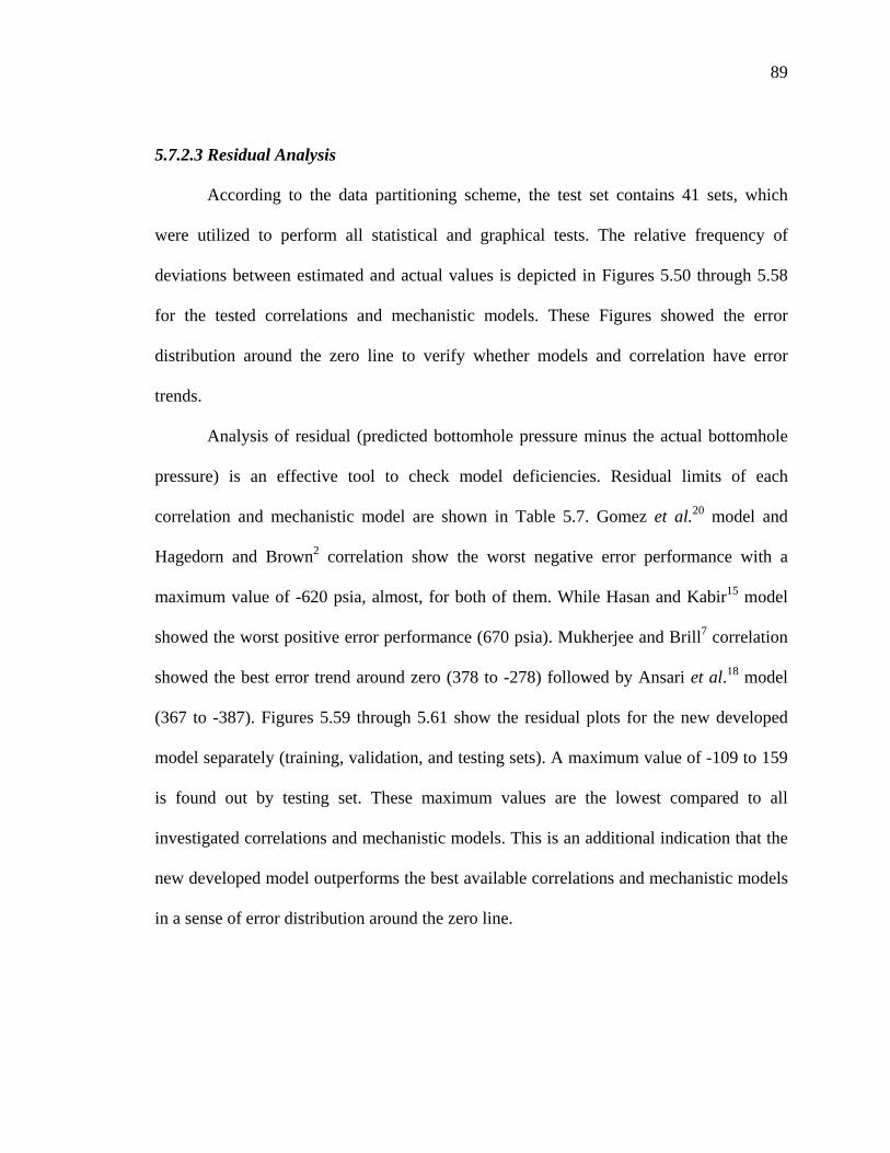
89
5.7.2.3 Residual Analysis
According to the data partitioning scheme, the test set contains 41 sets, which
were utilized to perform all statistical and graphical tests. The relative frequency of
deviations between estimated and actual values is depicted in Figures 5.50 through 5.58
for the tested correlations and mechanistic models. These Figures showed the error
distribution around the zero line to verify whether models and correlation have error
trends.
Analysis of residual (predicted bottomhole pressure minus the actual bottomhole
pressure) is an effective tool to check model deficiencies. Residual limits of each
correlation and mechanistic model are shown in Table 5.7. Gomez et al.20 model and
Hagedorn and Brown2 correlation show the worst negative error performance with a
maximum value of -620 psia, almost, for both of them. While Hasan and Kabir15 model
showed the worst positive error performance (670 psia). Mukherjee and Brill7 correlation
showed the best error trend around zero (378 to -278) followed by Ansari et al.18 model
(367 to -387). Figures 5.59 through 5.61 show the residual plots for the new developed
model separately (training, validation, and testing sets). A maximum value of -109 to 159
is found out by testing set. These maximum values are the lowest compared to all
investigated correlations and mechanistic models. This is an additional indication that the
new developed model outperforms the best available correlations and mechanistic models
in a sense of error distribution around the zero line.
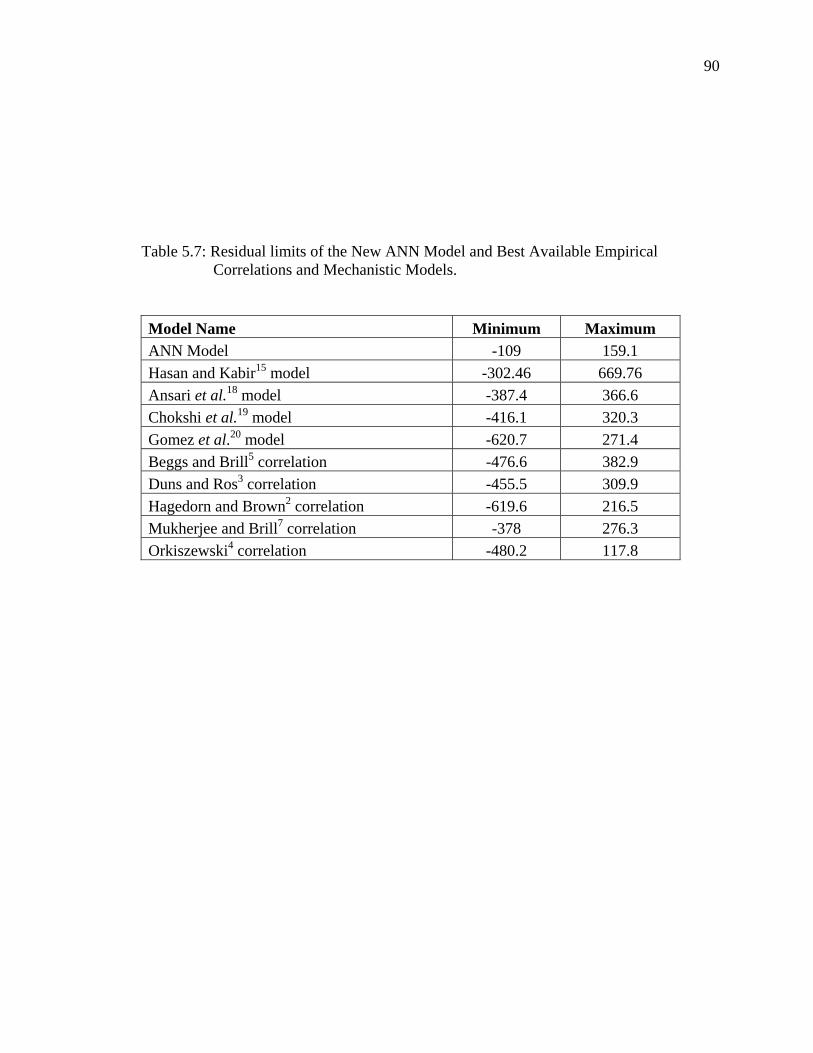
90
Table 5.7: Residual limits of the New ANN Model and Best Available Empirical Correlations and Mechanistic Models.
Model Name Minimum Maximum ANN Model -109 159.1 Hasan and Kabir15 model -302.46 669.76 Ansari et al.18 model -387.4 366.6 Chokshi et al.19 model -416.1 320.3 Gomez et al.20 model -620.7 271.4 Beggs and Brill5 correlation -476.6 382.9 Duns and Ros3 correlation -455.5 309.9 Hagedorn and Brown2 correlation -619.6 216.5 Mukherjee and Brill7 correlation -378 276.3 Orkiszewski4 correlation -480.2 117.8
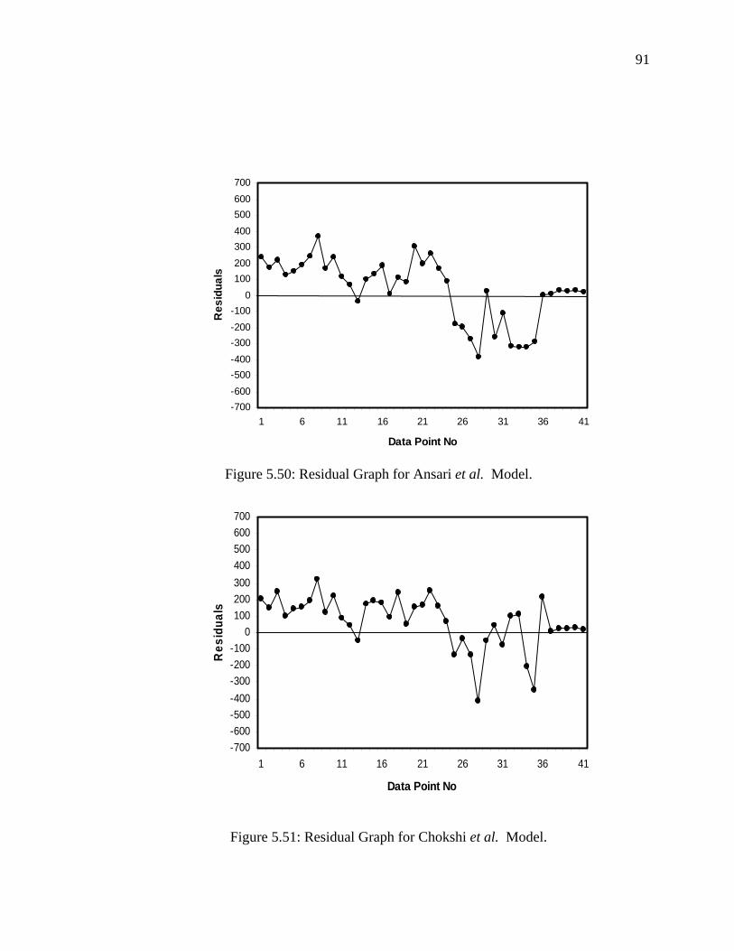
91
-700-600-500-400-300-200-100
0100200300400500600700
1 6 11 16 21 26 31 36 41
Data Point No
Res
idua
ls
Figure 5.50: Residual Graph for Ansari et al. Model.
-700-600-500-400-300-200-100
0100200300400500600700
1 6 11 16 21 26 31 36 41
Data Point No
Res
idua
ls
Figure 5.51: Residual Graph for Chokshi et al. Model.
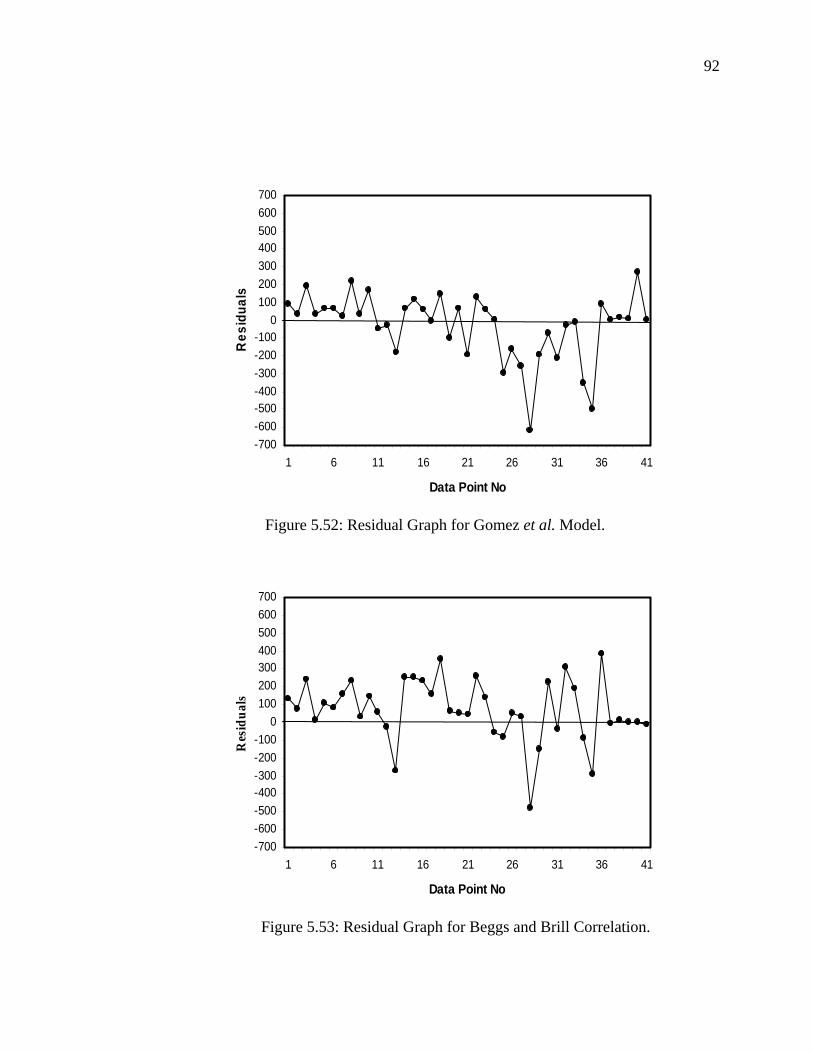
92
-700-600-500-400-300-200-100
0100200300400500600700
1 6 11 16 21 26 31 36 41
Data Point No
Res
idua
ls
Figure 5.52: Residual Graph for Gomez et al. Model.
-700-600-500-400-300-200-100
0100200300400500600700
1 6 11 16 21 26 31 36 41
Data Point No
Res
idua
ls
Figure 5.53: Residual Graph for Beggs and Brill Correlation.
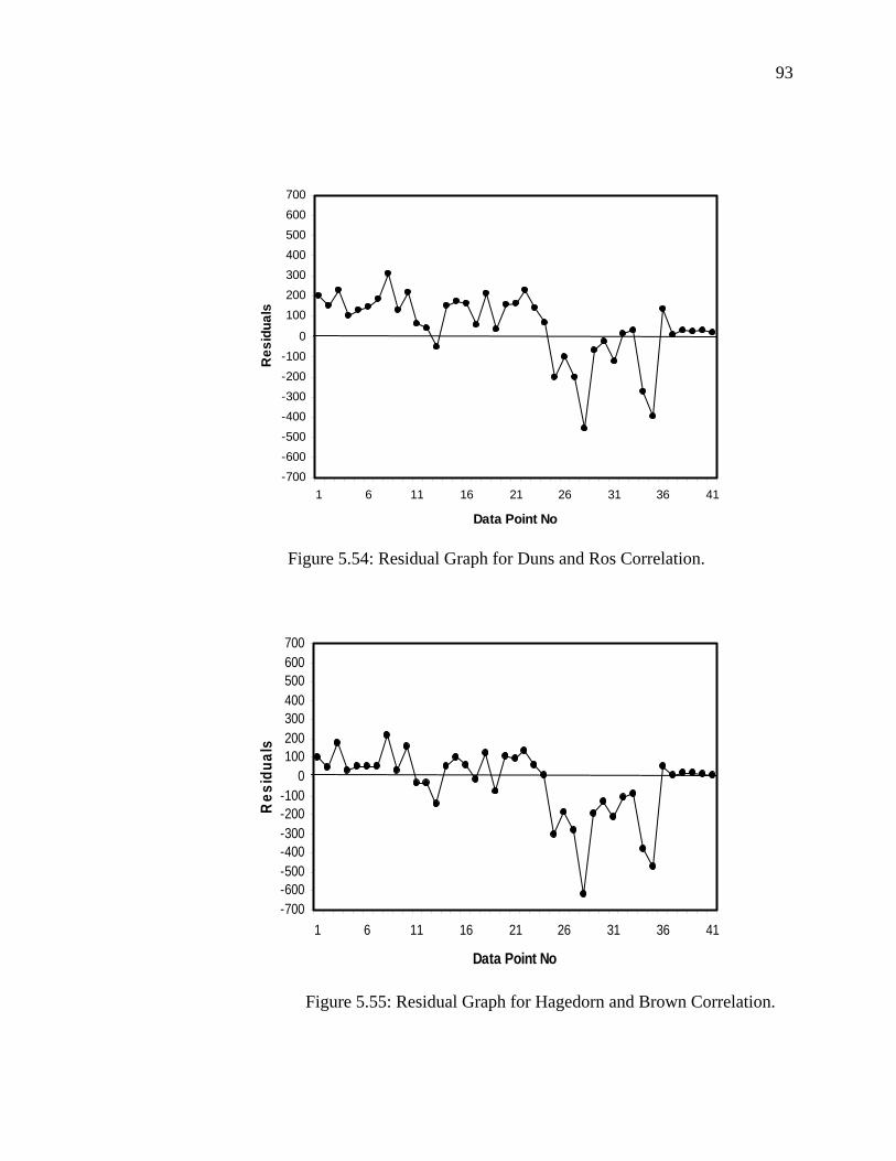
93
-700-600-500-400-300-200-100
0
100200300400500600700
1 6 11 16 21 26 31 36 41
Data Point No
Res
idua
ls
Figure 5.54: Residual Graph for Duns and Ros Correlation.
-700-600-500-400-300-200-100
0100200300400500600700
1 6 11 16 21 26 31 36 41
Data Point No
Res
idua
ls
Figure 5.55: Residual Graph for Hagedorn and Brown Correlation.
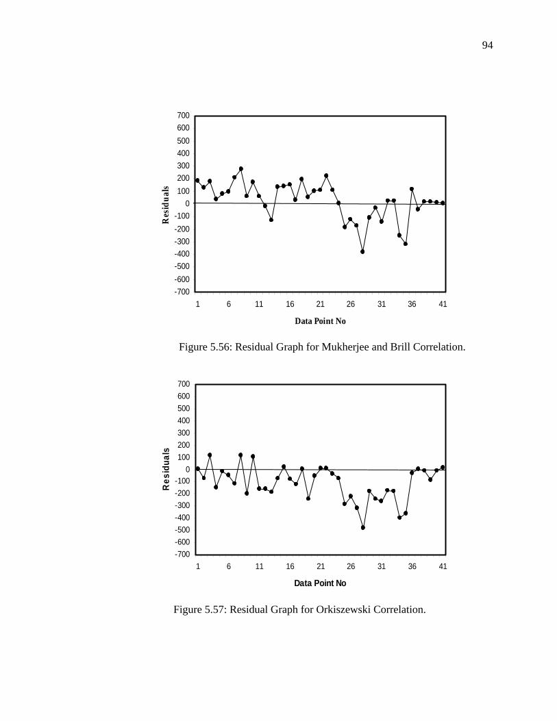
94
-700-600-500-400-300-200-100
0100200300400500600700
1 6 11 16 21 26 31 36 41
Data Point No
Res
idua
ls
Figure 5.56: Residual Graph for Mukherjee and Brill Correlation.
-700-600-500-400-300-200-100
0100200300400500600700
1 6 11 16 21 26 31 36 41
Data Point No
Res
idua
ls
Figure 5.57: Residual Graph for Orkiszewski Correlation.
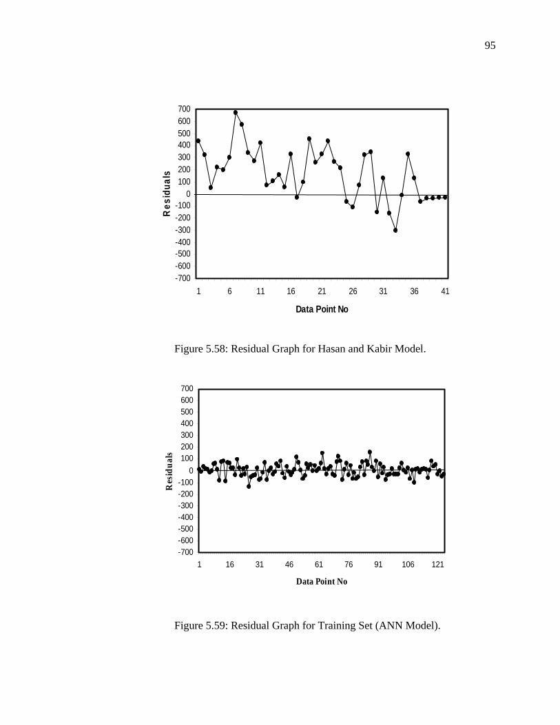
95
-700-600-500-400-300-200-100
0100200300400500600700
1 6 11 16 21 26 31 36 41
Data Point No
Res
idua
ls
Figure 5.58: Residual Graph for Hasan and Kabir Model.
-700-600-500-400-300-200-100
0100200300400500600700
1 16 31 46 61 76 91 106 121
Data Point No
Res
idua
ls
Figure 5.59: Residual Graph for Training Set (ANN Model).
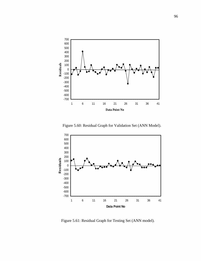
96
-700-600-500-400-300-200-100
0100200300400500600700
1 6 11 16 21 26 31 36 41
Data Point No
Res
idua
ls
Figure 5.60: Residual Graph for Validation Set (ANN Model).
-700-600-500-400-300-200-100
0100200300400500600700
1 6 11 16 21 26 31 36 41
Data Point No
Res
idua
ls
Figure 5.61: Residual Graph for Testing Set (ANN model).

97
CHAPTRE 6
CONCLUSIONS AND RECOMMENDATIONS
6.1 CONCLUSIONS
Based on the results and discussion presented in this study, the following conclusions
can be drawn:
1. Artificial Neural Network technique; specifically back-propagation learning
algorithm has been used successfully in developing a model for predicting flowing
bottomhole pressure in vertical wells.
2. The developed model outperformed the best available empirical correlations and
mechanistic models.
3. The developed model achieved best correlation coefficient (0.9735), the lowest
maximum absolute relative error (7.1401%), the lowest root mean squared error
(2.8013), the lowest standard error deviation (66.2448), and the lowest average
absolute percent error (2.1654%).
4. The model consistency has been checked through using a query data after training
and fixing the weights.

98
5. An executable program has been developed after obtaining the weights from the
original program. It can be used for estimating pressure drop in vertical multiphase
wells.
6. A trend analysis showed that the developed model accurately predicts the physical
process.
7. The developed model could perform better if redundancy in data does not exist.
8. The new developed model results can only be used within the range of used data.
Caution should be taken beyond the range of used input variables.
6.2 RECOMMENDATIONS
The following recommendations are made as a possible extension of the present work
1. The model performance can be more improved through using another data set with
a wider range of variables.
2. Commingling horizontal, vertical, and inclined multiphase flow data may
contribute a lot in developing a universal model.
3. The importance of all input variables can be further investigated in a future work
to determine the most important parameters that are involved in estimating
bottomhole pressure in vertical wells; this may result in reducing the number of
input variables.
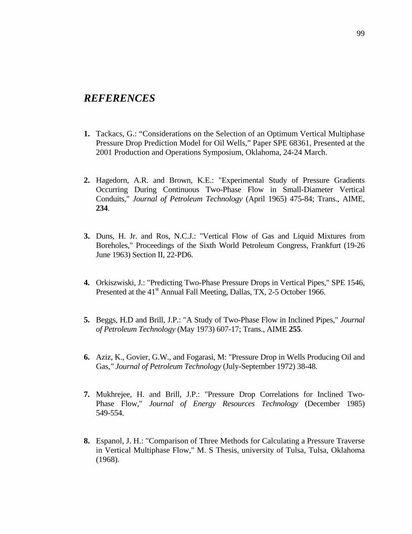
99
REFERENCES
1. Tackacs, G.: “Considerations on the Selection of an Optimum Vertical Multiphase
Pressure Drop Prediction Model for Oil Wells,” Paper SPE 68361, Presented at the 2001 Production and Operations Symposium, Oklahoma, 24-24 March.
2. Hagedorn, A.R. and Brown, K.E.: "Experimental Study of Pressure Gradients
Occurring During Continuous Two-Phase Flow in Small-Diameter Vertical Conduits," Journal of Petroleum Technology (April 1965) 475-84; Trans., AIME, 234.
3. Duns, H. Jr. and Ros, N.C.J.: "Vertical Flow of Gas and Liquid Mixtures from
Boreholes," Proceedings of the Sixth World Petroleum Congress, Frankfurt (19-26 June 1963) Section II, 22-PD6.
4. Orkiszwiski, J.: "Predicting Two-Phase Pressure Drops in Vertical Pipes," SPE 1546,
Presented at the 41st Annual Fall Meeting, Dallas, TX, 2-5 October 1966.
5. Beggs, H.D and Brill, J.P.: "A Study of Two-Phase Flow in Inclined Pipes," Journal
of Petroleum Technology (May 1973) 607-17; Trans., AIME 255. 6. Aziz, K., Govier, G.W., and Fogarasi, M: "Pressure Drop in Wells Producing Oil and
Gas," Journal of Petroleum Technology (July-September 1972) 38-48. 7. Mukhrejee, H. and Brill, J.P.: "Pressure Drop Correlations for Inclined Two-
Phase Flow," Journal of Energy Resources Technology (December 1985) 549-554.
8. Espanol, J. H.: "Comparison of Three Methods for Calculating a Pressure Traverse
in Vertical Multiphase Flow," M. S Thesis, university of Tulsa, Tulsa, Oklahoma (1968).
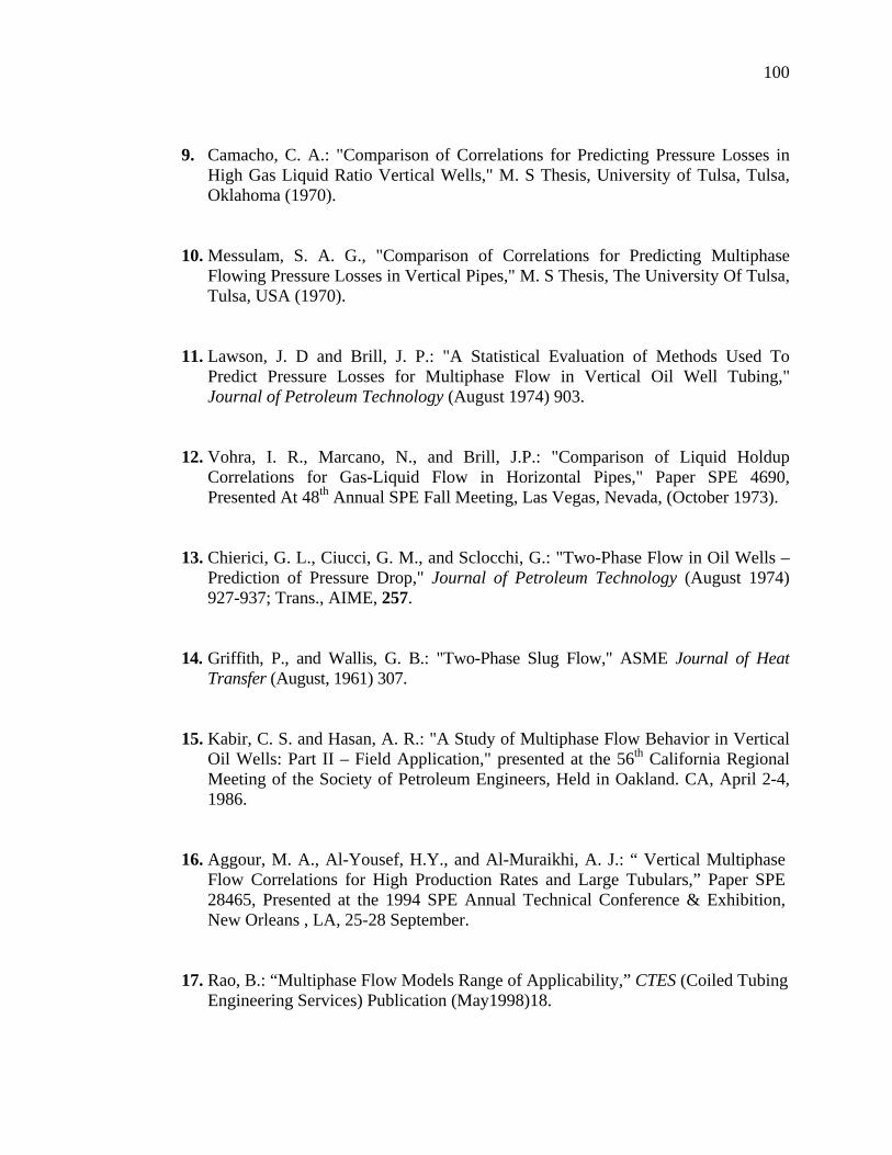
100
9. Camacho, C. A.: "Comparison of Correlations for Predicting Pressure Losses in High Gas Liquid Ratio Vertical Wells," M. S Thesis, University of Tulsa, Tulsa, Oklahoma (1970).
10. Messulam, S. A. G., "Comparison of Correlations for Predicting Multiphase
Flowing Pressure Losses in Vertical Pipes," M. S Thesis, The University Of Tulsa, Tulsa, USA (1970).
11. Lawson, J. D and Brill, J. P.: "A Statistical Evaluation of Methods Used To
Predict Pressure Losses for Multiphase Flow in Vertical Oil Well Tubing," Journal of Petroleum Technology (August 1974) 903.
12. Vohra, I. R., Marcano, N., and Brill, J.P.: "Comparison of Liquid Holdup
Correlations for Gas-Liquid Flow in Horizontal Pipes," Paper SPE 4690, Presented At 48th Annual SPE Fall Meeting, Las Vegas, Nevada, (October 1973).
13. Chierici, G. L., Ciucci, G. M., and Sclocchi, G.: "Two-Phase Flow in Oil Wells –
Prediction of Pressure Drop," Journal of Petroleum Technology (August 1974) 927-937; Trans., AIME, 257.
14. Griffith, P., and Wallis, G. B.: "Two-Phase Slug Flow," ASME Journal of Heat
Transfer (August, 1961) 307.
15. Kabir, C. S. and Hasan, A. R.: "A Study of Multiphase Flow Behavior in Vertical
Oil Wells: Part II – Field Application," presented at the 56th California Regional Meeting of the Society of Petroleum Engineers, Held in Oakland. CA, April 2-4, 1986.
16. Aggour, M. A., Al-Yousef, H.Y., and Al-Muraikhi, A. J.: “ Vertical Multiphase
Flow Correlations for High Production Rates and Large Tubulars,” Paper SPE 28465, Presented at the 1994 SPE Annual Technical Conference & Exhibition, New Orleans , LA, 25-28 September.
17. Rao, B.: “Multiphase Flow Models Range of Applicability,” CTES (Coiled Tubing
Engineering Services) Publication (May1998)18.
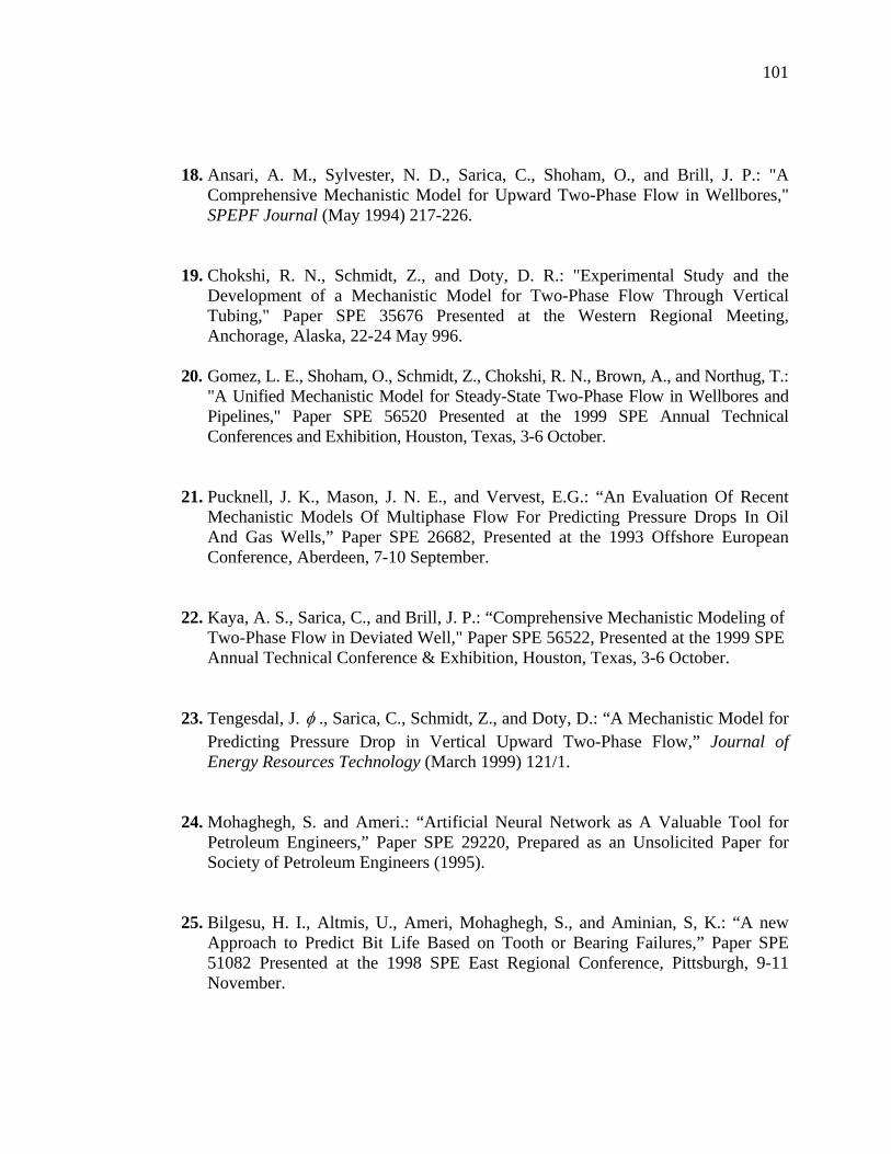
101
18. Ansari, A. M., Sylvester, N. D., Sarica, C., Shoham, O., and Brill, J. P.: "A
Comprehensive Mechanistic Model for Upward Two-Phase Flow in Wellbores," SPEPF Journal (May 1994) 217-226.
19. Chokshi, R. N., Schmidt, Z., and Doty, D. R.: "Experimental Study and the
Development of a Mechanistic Model for Two-Phase Flow Through Vertical Tubing," Paper SPE 35676 Presented at the Western Regional Meeting, Anchorage, Alaska, 22-24 May 996.
20. Gomez, L. E., Shoham, O., Schmidt, Z., Chokshi, R. N., Brown, A., and Northug, T.:
"A Unified Mechanistic Model for Steady-State Two-Phase Flow in Wellbores and Pipelines," Paper SPE 56520 Presented at the 1999 SPE Annual Technical Conferences and Exhibition, Houston, Texas, 3-6 October.
21. Pucknell, J. K., Mason, J. N. E., and Vervest, E.G.: “An Evaluation Of Recent
Mechanistic Models Of Multiphase Flow For Predicting Pressure Drops In Oil And Gas Wells,” Paper SPE 26682, Presented at the 1993 Offshore European Conference, Aberdeen, 7-10 September.
22. Kaya, A. S., Sarica, C., and Brill, J. P.: “Comprehensive Mechanistic Modeling of
Two-Phase Flow in Deviated Well," Paper SPE 56522, Presented at the 1999 SPE Annual Technical Conference & Exhibition, Houston, Texas, 3-6 October.
23. Tengesdal, J. φ ., Sarica, C., Schmidt, Z., and Doty, D.: “A Mechanistic Model for
Predicting Pressure Drop in Vertical Upward Two-Phase Flow,” Journal of Energy Resources Technology (March 1999) 121/1.
24. Mohaghegh, S. and Ameri.: “Artificial Neural Network as A Valuable Tool for
Petroleum Engineers,” Paper SPE 29220, Prepared as an Unsolicited Paper for Society of Petroleum Engineers (1995).
25. Bilgesu, H. I., Altmis, U., Ameri, Mohaghegh, S., and Aminian, S, K.: “A new
Approach to Predict Bit Life Based on Tooth or Bearing Failures,” Paper SPE 51082 Presented at the 1998 SPE East Regional Conference, Pittsburgh, 9-11 November.
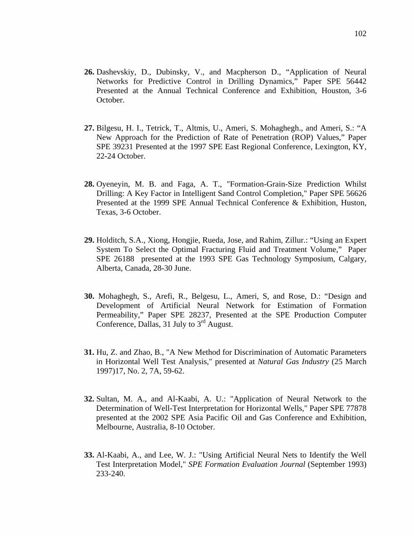
102
26. Dashevskiy, D., Dubinsky, V., and Macpherson D., “Application of Neural Networks for Predictive Control in Drilling Dynamics,” Paper SPE 56442 Presented at the Annual Technical Conference and Exhibition, Houston, 3-6 October.
27. Bilgesu, H. I., Tetrick, T., Altmis, U., Ameri, S. Mohaghegh., and Ameri, S.: “A New Approach for the Prediction of Rate of Penetration (ROP) Values,” Paper SPE 39231 Presented at the 1997 SPE East Regional Conference, Lexington, KY, 22-24 October.
28. Oyeneyin, M. B. and Faga, A. T., "Formation-Grain-Size Prediction Whilst Drilling: A Key Factor in Intelligent Sand Control Completion," Paper SPE 56626 Presented at the 1999 SPE Annual Technical Conference & Exhibition, Huston, Texas, 3-6 October.
29. Holditch, S.A., Xiong, Hongjie, Rueda, Jose, and Rahim, Zillur.: “Using an Expert
System To Select the Optimal Fracturing Fluid and Treatment Volume,” Paper SPE 26188 presented at the 1993 SPE Gas Technology Symposium, Calgary, Alberta, Canada, 28-30 June.
30. Mohaghegh, S., Arefi, R., Belgesu, L., Ameri, S, and Rose, D.: “Design and
Development of Artificial Neural Network for Estimation of Formation Permeability,” Paper SPE 28237, Presented at the SPE Production Computer Conference, Dallas, 31 July to 3rd August.
31. Hu, Z. and Zhao, B., "A New Method for Discrimination of Automatic Parameters
in Horizontal Well Test Analysis," presented at Natural Gas Industry (25 March 1997)17, No. 2, 7A, 59-62.
32. Sultan, M. A., and Al-Kaabi, A. U.: "Application of Neural Network to the Determination of Well-Test Interpretation for Horizontal Wells," Paper SPE 77878 presented at the 2002 SPE Asia Pacific Oil and Gas Conference and Exhibition, Melbourne, Australia, 8-10 October.
33. Al-Kaabi, A., and Lee, W. J.: "Using Artificial Neural Nets to Identify the Well Test Interpretation Model," SPE Formation Evaluation Journal (September 1993) 233-240.
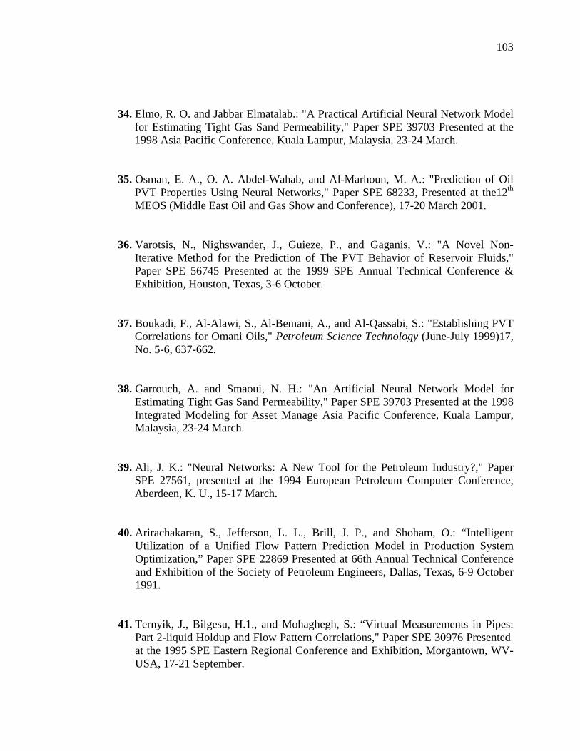
103
34. Elmo, R. O. and Jabbar Elmatalab.: "A Practical Artificial Neural Network Model
for Estimating Tight Gas Sand Permeability," Paper SPE 39703 Presented at the 1998 Asia Pacific Conference, Kuala Lampur, Malaysia, 23-24 March.
35. Osman, E. A., O. A. Abdel-Wahab, and Al-Marhoun, M. A.: "Prediction of Oil
PVT Properties Using Neural Networks," Paper SPE 68233, Presented at the12th MEOS (Middle East Oil and Gas Show and Conference), 17-20 March 2001.
36. Varotsis, N., Nighswander, J., Guieze, P., and Gaganis, V.: "A Novel Non-Iterative Method for the Prediction of The PVT Behavior of Reservoir Fluids," Paper SPE 56745 Presented at the 1999 SPE Annual Technical Conference & Exhibition, Houston, Texas, 3-6 October.
37. Boukadi, F., Al-Alawi, S., Al-Bemani, A., and Al-Qassabi, S.: "Establishing PVT Correlations for Omani Oils," Petroleum Science Technology (June-July 1999)17, No. 5-6, 637-662.
38. Garrouch, A. and Smaoui, N. H.: "An Artificial Neural Network Model for
Estimating Tight Gas Sand Permeability," Paper SPE 39703 Presented at the 1998 Integrated Modeling for Asset Manage Asia Pacific Conference, Kuala Lampur, Malaysia, 23-24 March.
39. Ali, J. K.: "Neural Networks: A New Tool for the Petroleum Industry?," Paper
SPE 27561, presented at the 1994 European Petroleum Computer Conference, Aberdeen, K. U., 15-17 March.
40. Arirachakaran, S., Jefferson, L. L., Brill, J. P., and Shoham, O.: “Intelligent Utilization of a Unified Flow Pattern Prediction Model in Production System Optimization,” Paper SPE 22869 Presented at 66th Annual Technical Conference and Exhibition of the Society of Petroleum Engineers, Dallas, Texas, 6-9 October 1991.
41. Ternyik, J., Bilgesu, H.1., and Mohaghegh, S.: “Virtual Measurements in Pipes:
Part 2-liquid Holdup and Flow Pattern Correlations," Paper SPE 30976 Presented at the 1995 SPE Eastern Regional Conference and Exhibition, Morgantown, WV-USA, 17-21 September.
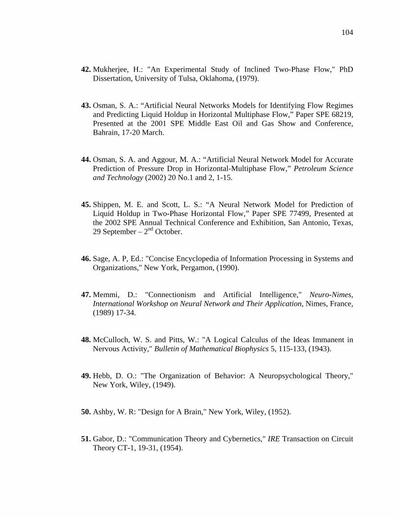
104
42. Mukherjee, H.: "An Experimental Study of Inclined Two-Phase Flow," PhD Dissertation, University of Tulsa, Oklahoma, (1979).
43. Osman, S. A.: “Artificial Neural Networks Models for Identifying Flow Regimes
and Predicting Liquid Holdup in Horizontal Multiphase Flow,” Paper SPE 68219, Presented at the 2001 SPE Middle East Oil and Gas Show and Conference, Bahrain, 17-20 March.
44. Osman, S. A. and Aggour, M. A.: “Artificial Neural Network Model for Accurate Prediction of Pressure Drop in Horizontal-Multiphase Flow,” Petroleum Science and Technology (2002) 20 No.1 and 2, 1-15.
45. Shippen, M. E. and Scott, L. S.: “A Neural Network Model for Prediction of
Liquid Holdup in Two-Phase Horizontal Flow,” Paper SPE 77499, Presented at the 2002 SPE Annual Technical Conference and Exhibition, San Antonio, Texas, 29 September – 2nd October.
46. Sage, A. P, Ed.: "Concise Encyclopedia of Information Processing in Systems and
Organizations," New York, Pergamon, (1990). 47. Memmi, D.: "Connectionism and Artificial Intelligence," Neuro-Nimes,
International Workshop on Neural Network and Their Application, Nimes, France, (1989) 17-34.
48. McCulloch, W. S. and Pitts, W.: "A Logical Calculus of the Ideas Immanent in
Nervous Activity," Bulletin of Mathematical Biophysics 5, 115-133, (1943). 49. Hebb, D. O.: "The Organization of Behavior: A Neuropsychological Theory,"
New York, Wiley, (1949).
50. Ashby, W. R: "Design for A Brain," New York, Wiley, (1952).
51. Gabor, D.: "Communication Theory and Cybernetics," IRE Transaction on Circuit Theory CT-1, 19-31, (1954).
105
52. Rosenblatt, F.: "The Preceptron: A Probabilistic Model for Information Storage and Organization in the Brain," Psychological Review 65, 386-408, (1958).
53. Minsky, M. L. and Papert, S. A.: "Preceptrons," Cambridge, MA. MT Press, (1969).
54. Rumelhart, D. E., Hinton, G. E., and Williams, R. J.: "Learning Representations by Back-Propagation Errors," Nature, London, 323 (1986) 533-536.
55. Haykin, S.: "Neural Network: A Comprehensive Foundation," Macmillan Publishing Company, NJ, Lehigh Press, (1994).
56. Aleksander. I. and Morton, H.: "An Introduction to Neural Computing," London, Chapman & Hall, (1990).
57. Shepherd, G. M. and Koch, C.: "Introduction to Synaptic Circuits," in the Synaptic Organization of the Brain. New York, Oxford University Press, (1990) 3-31.
58. James, A. Freeman and David, M. Skapura.: "Neural Networks: Algorithms, Applications, and Programming Techniques," Addison-Wesley Publishing Company, (1991).
59. Elman, J.L.: “Finding Structure in Time,” Cognitive Science, (1990) 14,179-211.
60. Kramer, A. H. and Sangiovanni, V. A.: "Efficient Parallel Learning Algorithms for Neural Networks," in Advances in Neural Information Processing Systems 1 (D. S. Touretzky, Edition), San Mateo, CA, Morgan Kaufmann. (1989) 40-78.
61. Rai, R., Singh, I., and Srini-Vasan, S.: "Comparison of Multiphase Flow
Correlations with Measured Field Data of Vertical and Deviated Oil Wells in India," SPE PE (August 1989) 341-8.
62. Simon Haykin.: "Neural Network: A Comprehensive Foundation," Upper Saddle River, NJ, Prentice Hall (1999).
106
63. "MATLAB," Mathwork, Neural Network Toolbox Tutorial, (http://www.mathtools.net/MATLAB/Neural_Networks/index.html).
64. Minsky, M. L. and Papert, S. A.: "Preceptrons," Expanded Edition. Cambridge, MA. MT Press, (1988).
65. Gori, M. and Tesi, A.: "On the Problem of Local Minima in Back-Propagation," IEEE Transactions on Pattern Analysis and Machine Intelligence (1992)14, 76-86.
66. Taitel, Y. and Duckler, A. E.: "A Model for Predicting Flow Regime Transitions in
Horizontal and Near Horizontal Gas-Liquid Flow," AIChE Journal (1976) 22, No. 1, 47-55.
67. Barnea, D.: "A Unified Model for Predicting Flow Pattern Transitions for the Whole
Range of Pipe Inclinations," International Journal of Multiphase Flow (1987)13, No. 1,1-12.
68. Taitel, Y. and Barnea, D.: "Two-Phase Slug Flow," Academic Press Inc. (1990). 69. Scott, S. L., Shoham, O., and Brill, J. P.: "Prediction of Slug Length in Horizontal
Large-Diameter Pipes," SPE Production Engineering (August 1989) 335-340.
70. Alves, I., N., Caetano, E. F., Minami, K., and Shoham, O.: "Modeling Annular Flow Behavior for Gas Wells," SPE Production Engineering (November 1991) 435-440.
APPENDIX A
EMPIRICAL CORRELATIONS AND
MECHANISTIC MODELS

A-1
APPENDIX A
EMPIRICAL CORRELATIONS AND MECHANISTIC MODELS
This appendix is divided into two sections. A detailed review of the most
commonly used vertical multiphase flow empirical correlations is presented in section
A.1 whereas a detailed discussion of the three evaluated mechanistic models is
presented in section A.2.
A.1 Vertical Multiphase Flow Empirical Correlations
Some of the most used vertical multiphase empirical correlations will be
discussed thoroughly in the next section. Those are; modified Hagedorn & Brown2,
Duns & Ros3, Orkiszweski4, Beggs & Brill5, Aziz & Govier6, and Mukhrejee & Brill7
A.1.1 Generalized Correlation of Hagedorn and Brown (1965):
Hagedorn and Brown2 correlation is a semi empirical method based on the
original work of Hagedorn and Brown in 1964 with the addition of a correlation for
liquid hold up. It incorporated general energy equation and 1500 ft test well data.
General energy equation defined summation of three terms to be equal to the total
pressure gradient in pipes, which includes hydrostatic gradient, friction gradient, and
acceleration gradient. These terms can be stated in Equation (1) below.
onacceleratifrictionelevationtotal dhdP
dhdP
dhdP
dhdP
⎟⎠⎞
⎜⎝⎛+⎟
⎠⎞
⎜⎝⎛+⎟
⎠⎞
⎜⎝⎛=⎟
⎠⎞
⎜⎝⎛
The previous equation can be written in a detailed form as;
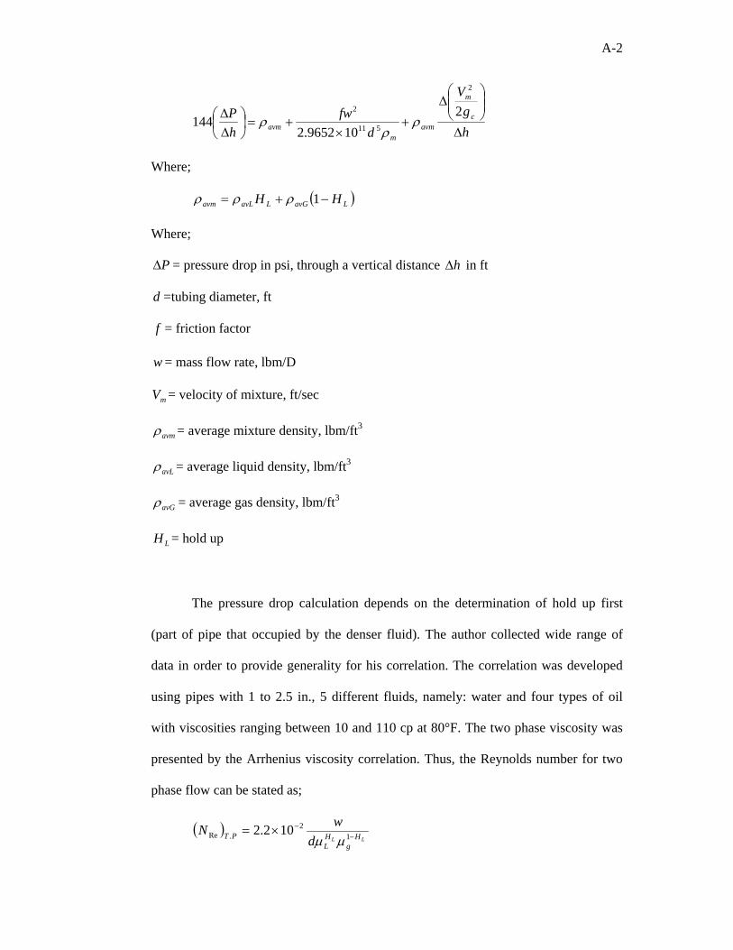
A-2
hg
V
dfw
hP c
m
avmm
avm ∆
⎟⎟⎠
⎞⎜⎜⎝
⎛∆
+×
+=⎟⎠⎞
⎜⎝⎛∆∆ 2
109652.2144
2
511
2
ρρ
ρ
Where;
( )LavGLavLavm HH −+= 1ρρρ
Where;
P∆ = pressure drop in psi, through a vertical distance h∆ in ft
d =tubing diameter, ft
f = friction factor
w = mass flow rate, lbm/D
mV = velocity of mixture, ft/sec
avmρ = average mixture density, lbm/ft3
avLρ = average liquid density, lbm/ft3
avGρ = average gas density, lbm/ft3
LH = hold up
The pressure drop calculation depends on the determination of hold up first
(part of pipe that occupied by the denser fluid). The author collected wide range of
data in order to provide generality for his correlation. The correlation was developed
using pipes with 1 to 2.5 in., 5 different fluids, namely: water and four types of oil
with viscosities ranging between 10 and 110 cp at 80°F. The two phase viscosity was
presented by the Arrhenius viscosity correlation. Thus, the Reynolds number for two
phase flow can be stated as;
( )LL H
gHL
PT dwN −
−×= 12
.Re 102.2µµ
A-3
Where;
( ) PTN .Re = Reynolds number for two phase flow
Lµ = liquid viscosity, Cp, and
gµ = gas viscosity, Cp
The developed correlation does not recognize flow regimes. However, assuming
one flow pattern for the whole pipe weakened the correlation where different flow
patterns are observed along the length of the pipe and the pressure losses vary
accordingly. In other words, the correlation ignored the variation of flow patterns,
which significantly affect the pressure loss calculations. The calculation of the liquid
holdup depends on four dimensionless numbers which are the liquid velocity number, the
gas velocity number, the pipe diameter number and the liquid viscosity number listed
below:
41
⎟⎟⎠
⎞⎜⎜⎝
⎛=
σρg
VN LsLLV
41
⎟⎟⎠
⎞⎜⎜⎝
⎛=
σρg
VN LsggV
21
⎟⎠⎞
⎜⎝⎛=σρ g
dN LD
41
3 ⎟⎟⎠
⎞⎜⎜⎝
⎛=
σρµ
LLL
gN
Where;
LVN = liquid-velocity number
gVN = gas-velocity number
DN = pipe-diameter number

A-4
LN = liquid-viscosity number
sLV = superficial liquid velocity, ft/sec
sgV = superficial gas velocity, ft/sec
Lρ = liquid density, lbm/ft3
σ = surface tension, lbm/sec2
The hold up is actually treated as a pseudo holdup that could be calculated by
taking into consideration the total pressure drop and friction factor that are calculated a
step before. Some modifications have been made to account for these shortcomings by
different investigators later on. Hagedorn and Brill made other adjustment including
calculation of mixture density using hold up correlation and comparing it with the
mixture density for no-slippage. The largest of these two values is then used.
A.1.2 Duns and Ros Correlation (1963):
The Duns & Ros3 correlation was developed using data from a large-scale,
carefully controlled laboratory facilities. The correlation was suitably modified using
field data for vertical flow of gas and liquid mixtures in wells. This correlation is valid
for a wide range of oil and gas mixtures and flow regimes. Based on the inlet
superficial gas and liquid velocities, the authors developed a chart to identify the various
flow regimes. The different flow regimes like single phase, bubble, plug, froth, slug,
transition and mist flow are grouped into three broad flow regions; these are; bubble
flow, slug flow, and mist flow. The different nature of these three main regions
necessitates separate correlations for friction and liquid holdup for each region. These
flow patterns could be defined using dimensionless groups described in the previous
A-5
section. Slippage effect and friction factor have been incorporated in the total pressure
gradient calculation for each flow pattern.
The following equations were used for each flow region:
Bubble Flow Region
Slip factor, 2
/321 1 ⎟⎟
⎠
⎞⎜⎜⎝
⎛−
++=LV
gVLV N
NFNFFs
dNFFF 4
3/
3 −=
Slip velocity, 5.0
938.1 ⎟⎟⎠
⎞⎜⎜⎝
⎛=
L
L
ssV
σρ
Where; groups essdimensionl are ,,,,,, 7654321 FFFFFFF
( ) ( )[ ]s
sLssLsgssLsgsL V
VVVVVVVVH
24
5.02 +−−+−−=
Duns and Ros suggested the following limit for bubble flow region:
( )LVgV NLLN 210 +≤≤
Slug Flow Region
Slip factor, ( ) ( )( )2
7
\6
982.0
5 11
LV
gV
NF
FNFs
+
++=
6\
6 029.0 FNFwhere
d +=
These dimensionless groups can be obtained from Figures A1 & A2
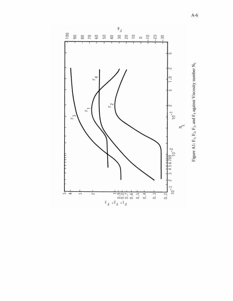
A-6
Figu
re A
1: F
1, F 2
, F3,
and
F 4 a
gain
st V
isco
sity
num
ber N
L
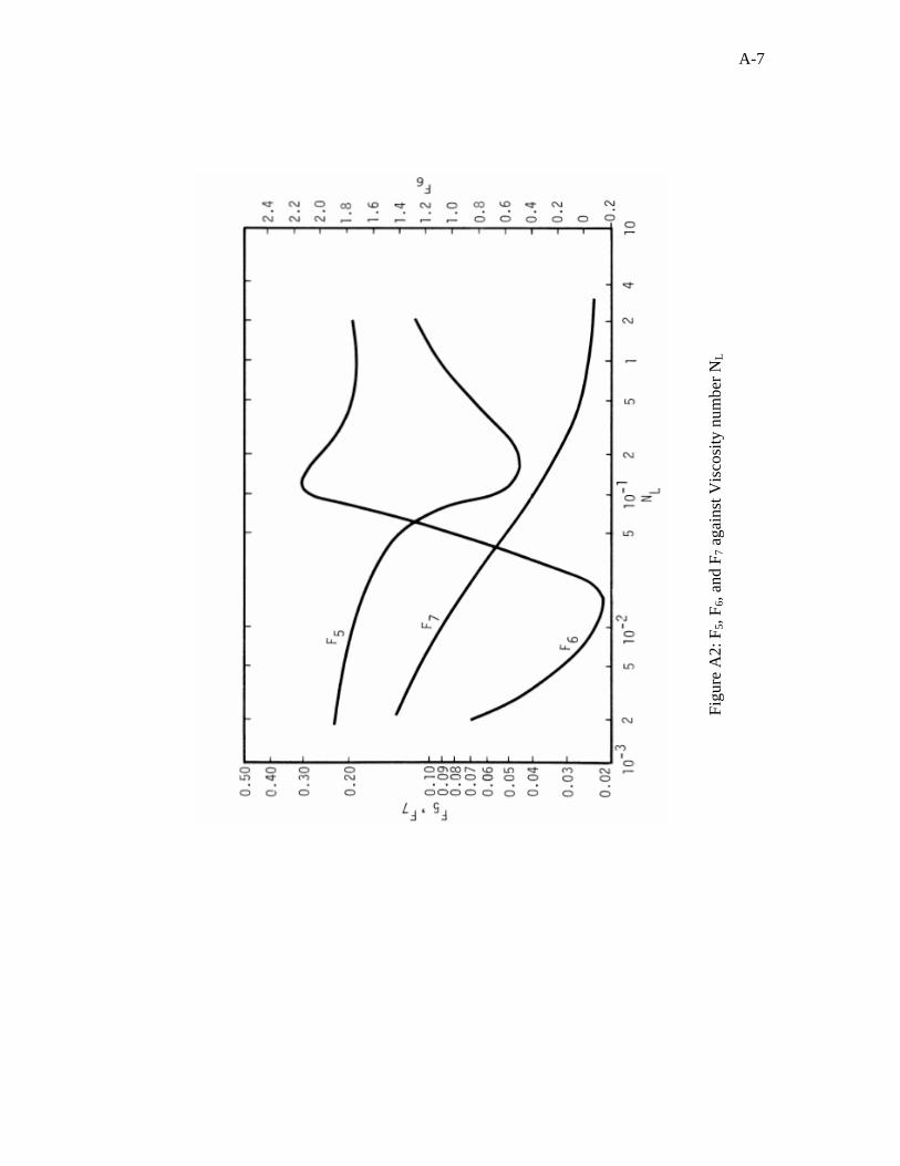
A-7
Figu
re A
2: F
5, F 6
, and
F7 a
gain
st V
isco
sity
num
ber N
L
A-8
The slip velocity and the holdup are similarly calculated using the bubble flow
regions corresponding equations.
Duns and Ros suggested the following limit for slug flow region:
( )LVgVLV NNNLL 365021 +<<+
Mist Flow Region:
Slip factor, zeros =
⎟⎟⎠
⎞⎜⎜⎝
⎛+
=
sL
sgL
VV
H1
1
The static gradient due to mixture flowing density is given by:
( )L
gLLst HHGρρ
−+= 1
Duns and Ros suggested the following limit for slug flow region:
( )75.08475 LVgV NN +>
d21 N offunction are , LL , and can be obtained from Figure A3
Each flow regime has its own friction factor correlation. For the bubble and slug
regimes, the friction gradient is calculated using the following equations:
⎟⎟⎠
⎞⎜⎜⎝
⎛+=⎟
⎠⎞
⎜⎝⎛
sL
sgsLLw
f VV
dVf
dzdP 1
24 2ρ
wf was formulated from the experimental data as follows:
3
21
fff
f w =
21 , ff can be obtained from Figures A4 & A5
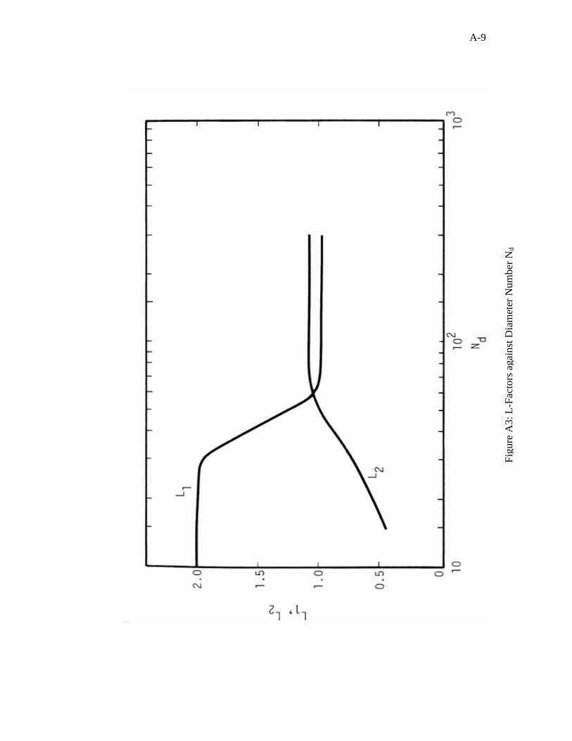
A-9
Figu
re A
3: L
-Fac
tors
aga
inst
Dia
met
er N
umbe
r Nd
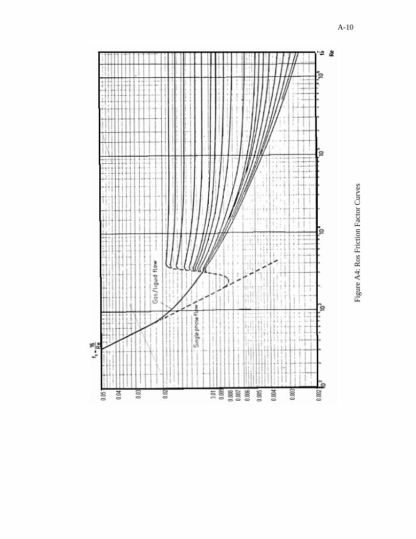
A-10
Figu
re A
4: R
os F
rictio
n Fa
ctor
Cur
ves
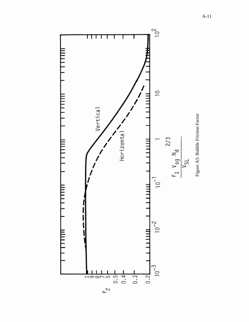
A-11
Figu
re A
5: B
ubbl
e Fr
ictio
n Fa
ctor
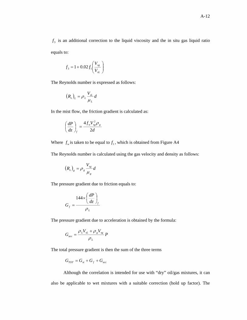
A-12
3f is an additional correction to the liquid viscosity and the in situ gas liquid ratio
equals to:
⎟⎟⎠
⎞⎜⎜⎝
⎛+=
sL
sg
VV
ff 13 02.01
The Reynolds number is expressed as follows:
( ) dV
RL
sLLLe µ
ρ=
In the mist flow, the friction gradient is calculated as:
dVf
dzdP gsgw
f 24 2 ρ
=⎟⎠⎞
⎜⎝⎛
Where wf is taken to be equal to 1f , which is obtained from Figure A4
The Reynolds number is calculated using the gas velocity and density as follows:
( ) dV
Rg
sggge µ
ρ=
The pressure gradient due to friction equals to:
L
ff
dzdP
Gρ
⎟⎠⎞
⎜⎝⎛×
=
144
The pressure gradient due to acceleration is obtained by the formula:
PVV
GL
sggsLLacc ρ
ρρ +=
The total pressure gradient is then the sum of the three terms
accfstTOT GGGG ++=
Although the correlation is intended for use with “dry” oil/gas mixtures, it can
also be applicable to wet mixtures with a suitable correction (hold up factor). The

A-13
method depends on assigning the flow region in order to better apply and obtain high
accuracy of flow profiles (pressure traverse). For water contents less than 10%, the
Duns-Ros correlation (with a correction factor) has been reported to work well in the
bubble, plug, and froth regions.
Pressure gradient was found to be independent of the gas flow rates at low liquid flow
rates but it varies considerably at higher liquid flow rates. Three types of correction
factors were proposed by Duns and Ros, which accounted for Reynolds number, high
gas-liquid ratios, and liquid viscosity. The pressure drop is over predicted at gas-liquid
ratios greater than 5000 scf/bbl.
A.1.3 Orkiszweski Correlation (1966):
In a detailed study of two-phase correlations, Orkiszweski4 compared the pressure
behavior predicted from various correlations using actual field data. He concluded that
no correlation worked sufficiently well for all flow regimes. He did, however, identify
several correlations that work well for specific flow regimes. He developed a correlation
which is basically an extension of Griffith & Wallis work. By using variations of
existing methods, he presented with an equation for pressure gradient calculation that
covered all four flow regimes (bubble, slug, annular-slug and mist). His method is
versatile and was validated using 148 measured pressure drops in actual wells.
Because slug flow is present in 95% of the studied cases, the author
recommended Griffith and Wallis for this flow pattern. It should be noted that the
liquid distribution coefficient (hold-up) is evaluated using the data from the Hagedorn
& Brown model. Duns and Ros correlation was used for transition and annular mist
flow, whenever it exists.
The pressure drop was expressed by Orkiszweski as:
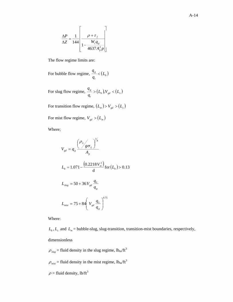
A-14
⎥⎥⎥⎥⎥
⎦
⎤
⎢⎢⎢⎢⎢
⎣
⎡
−
+=
∆∆
pAqWZ
P
p
gt
f
246371
1441 τρ
The flow regime limits are:
For bubble flow regime, ( )bt
g Lqq
<
For slug flow regime, ( ) ( )sgdbt
g LVLqq
<> ,
For transition flow regime, ( ) ( )sgdm LVL >>
For mist flow regime, ( )mgd LV >
Where;
p
L
L
ggd Ag
qV
41
⎟⎠⎞⎜
⎝⎛
=σ
ρ
( ) ( ) 13.0for d
2218.0071.1
2
>−= bm
b LV
L
g
Lgdslug q
qVL 3650 +=
75.0
8475 ⎟⎟⎠
⎞⎜⎜⎝
⎛+=
g
Lgdmist q
qVL
Where:
bL , sL and mL = bubble-slug, slug-transition, transition-mist boundaries, respectively,
dimensionless
slugρ = fluid density in the slug regime, lbm/ft3
mistρ = fluid density in the mist regime, lbm/ft3
ρ = fluid density, lb/ft3
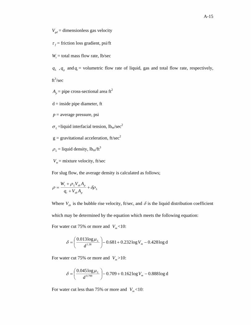
A-15
gdV = dimensionless gas velocity
fτ = friction loss gradient, psi/ft
tW = total mass flow rate, lb/sec
Lq , gq and tq = volumetric flow rate of liquid, gas and total flow rate, respectively,
ft3/sec
pA = pipe cross-sectional area ft2
d = inside pipe diameter, ft
p = average pressure, psi
Lσ =liquid interfacial tension, lbm/sec2
g = gravitational acceleration, ft/sec2
Lρ = liquid density, lbm/ft3
mV = mixture velocity, ft/sec
For slug flow, the average density is calculated as follows;
Lpsbt
psbLt
AVqAVW
δρρ
ρ ++
+=
Where sbV is the bubble rise velocity, ft/sec, and δ is the liquid distribution coefficient
which may be determined by the equation which meets the following equation:
For water cut 75% or more and mV <10:
d log428.0 log232.0681.0log013.0
38.1 −+−⎟⎠⎞
⎜⎝⎛= m
L Vd
µδ
For water cut 75% or more and mV >10:
d log888.0 log162.0709.0log045.0799.0 −+−⎟
⎠⎞
⎜⎝⎛= m
L Vd
µδ
For water cut less than 75% or more and mV <10:
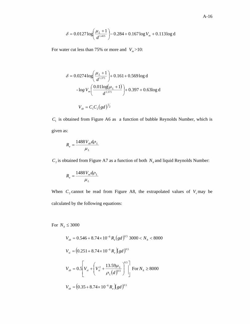
A-16
d log113.0 log167.0284.01
log0127.0 415.1 ++−⎟⎠⎞
⎜⎝⎛ +
= mL V
dµ
δ
For water cut less than 75% or more and mV >10:
( ) d 0.63log0.397
1log01.0 l -
d log569.0161.01log0274.0
571.1
371.1
++⎟⎠⎞
⎜⎝⎛ +
++⎟⎠⎞
⎜⎝⎛ +
=
dVog
d
Lm
L
µ
µδ
( ) 21
21 gdCCVsb =
1C is obtained from Figure A6 as a function of bubble Reynolds Number, which is
given as:
L
Lsbe
dVR
µρ 1488
=
2C is obtained from Figure A7 as a function of both bN and liquid Reynolds Number:
L
Lme
dVR
µρ 1488
=
When 2C cannot be read from Figure A8, the extrapolated values of sV may be
calculated by the following equations:
For 3000≤bN
( ) 5.061074.8546.0 gdRV esb−×+= 80003000 << bN
( )( ) 5.061074.8251.0 gdRV esi−×+=
( ) ⎥⎥⎦
⎤
⎢⎢⎣
⎡
⎟⎟⎠
⎞⎜⎜⎝
⎛++=
5.0
5.02 59.135.0
dVVV
L
Lsisisb ρ
µ For 8000≥bN
( )( ) 5.061074.835.0 gdRV esb−×+=
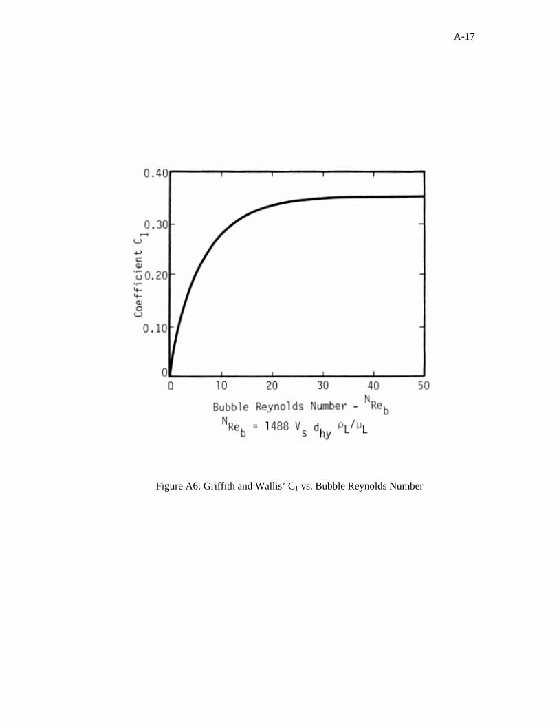
A-17
Figure A6: Griffith and Wallis’ C1 vs. Bubble Reynolds Number
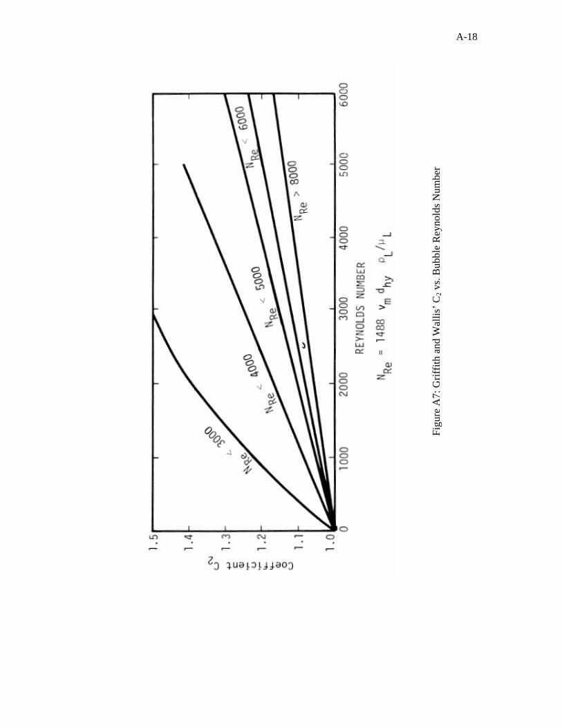
A-18
Figu
re A
7: G
riffit
h an
d W
allis
’ C2 v
s. B
ubbl
e R
eyno
lds N
umbe
r
A-19
The wall friction loss term is expressed as:
⎥⎥⎦
⎤
⎢⎢⎣
⎡+
+
+= δ
ρτ
psbt
psbL
c
mLf AVq
AVqdg
Vf2
2
The friction factor f is obtained from Moody Chart Figure A8
The Reynolds Number equation is as follows
L
Lme
dVR
µρ 1488
=
For mist flow regime, the wall friction loss term is expressed as:
dg
Vf
c
ggf 2
2ρτ =
In the bubble flow:
dg
Vf
c
LLf 2
2ρτ =
Where cg is the dimensionless conversion factor = 32.2 lbm/ft3
Griffith & Wallis14 and Duns and Ros4 correlations were found to be more
accurate than other tested methods. A combination of both methods was tested against
the 148 data set. Griffith & Wallis14 was shown more reliable in the lower flow rate
range of slug flow. However, Duns and Ros correlation gave the same result and failed
in higher viscosity oils in the low flow-rate range. Orkiszewski extended Griffith &
Wallis work to higher velocity ranges.
A.1.4 Aziz -Govier and Fogarasi Correlation (1972)
In this work, the authors conducted an extensive review of the best available
flow regimes formulae. Four flow patterns were recognized; those are bubble, slug,
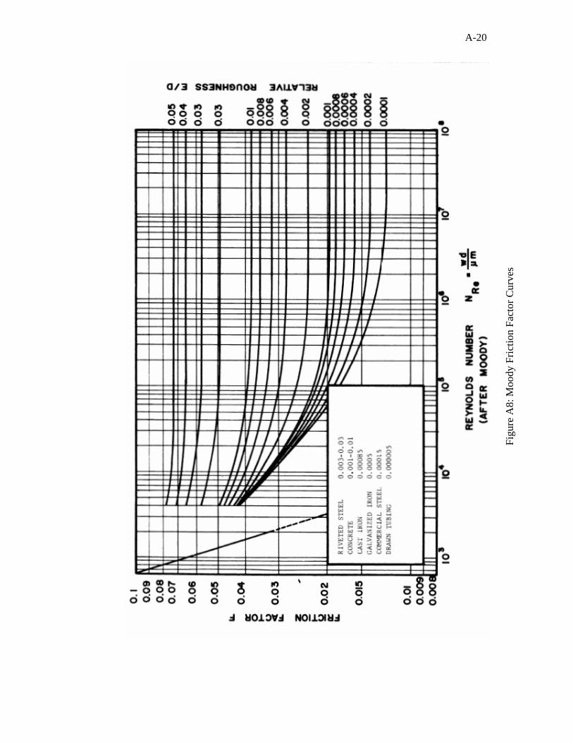
A-20
Figu
re A
8: M
oody
Fric
tion
Fact
or C
urve
s
A-21
transition, and mist. A flow pattern map was proposed as a result. The flow patterns
were identified based on dimensionless groups as follows:
41
31
4.6272
0764.0 ⎟⎟⎠
⎞⎜⎜⎝
⎛⎟⎟⎠
⎞⎜⎜⎝
⎛=
L
Lgsgx VN
σρρ
41
4.6272
⎟⎟⎠
⎞⎜⎜⎝
⎛=
L
LsLy VN
σρ
( ) 172.01 10051.0 yNN =
yNN 8.360.82 +=
( ) 152.03 10070 −= yNN
Where;
xN , yN are dimensionless group
321 ,, NNN are dimensionless boundary limits
Each flow regime had its own limit as follows:
Bubble Flow:
1NN y <
Slug Flow:
0.4Nfor y21 <<< NNN x
0.4Nfor 5.26 y1 ≥<< xNN
Transition Flow:
0.4Nfor y32 <<< NNN x
Mist Flow:
0.4Nfor y3 <> NN x
0.4Nfor 5.26 y >>yN
A-22
The two phase density for the bubble and slug flows was given by the following
equation:
ZdZdPP ms ∆⎟
⎠⎞
⎜⎝⎛=∆ ρ
( )LgLLm HH −+= 1ρρρ
⎥⎥⎦
⎤
⎢⎢⎣
⎡−=
bf
sgL V
VH 1
Where:
bfV is the bubble rise velocity under flowing condition, ft/sec
Various methods were used to obtain the rise velocity of the bubbles under
stagnant, bsV , and flowing, bfV , conditions
The acceleration was considered to be negligible in the bubble and slug flow
regimes.
To calculate the pressure gradient for the transition region, the pressure
gradients must be calculated using both the slug and mist flow equations; linear
interpolation is then performed as follows:
mistslugs dZ
dPBdZdPA
dZdPP ⎟
⎠⎞
⎜⎝⎛+⎟
⎠⎞
⎜⎝⎛=⎟
⎠⎞
⎜⎝⎛=∆
Where:
B& 23
2
23
3
NNNN
NNNN
A xx
−−
=−−
=
The Colebrook friction factor equation was used to calculate the pressure drop due to
frictions:
⎟⎟⎠
⎞⎜⎜⎝
⎛+−+=
fRdd
f eεε
235.91log448.3
2log41
Where ε is the wall roughness factor = 0.00015

A-23
To calculate the friction factor for the bubble flow, the friction gradient is given by the
following equation:
dgVf
dZdP
c
mm
f 2
2ρ=⎟
⎠⎞
⎜⎝⎛
The Reynolds number is given as;
( )L
mLe
dVR
µρ=
For the slug flow:
dgVHf
dZdP
c
mLL
s 2
2ρ=⎟
⎠⎞
⎜⎝⎛
The total pressure drop gradient is then can be expressed as:
sfTOT dZdP
dZdP
dZdP
⎟⎠⎞
⎜⎝⎛+⎟
⎠⎞
⎜⎝⎛=⎟
⎠⎞
⎜⎝⎛
A.1.5 Beggs & Brill Correlation (1973)
This method is probably the most widely used method because it can be applied
in vertical, horizontal, and inclined pipes. It was developed using experimental data in a
small scale experimental, test facility using 1 inch and 1.5 inches diameter pipes. This
correlation resulted from experiments using air and water as test fluids over a wide
range of parameters. The factors used for correlating are gas flow rate, liquid flow rate,
pipe diameter, inclination angle, liquid holdup, pressure gradient and horizontal flow
regime. The flow regime is determined based on the limits set for "no-slip" holdup and a
dimensionless number called the Froude number. A unique modification of the three
horizontal flow regime, as illustrated in Figure A9 was done. Further, different
correlations for liquid holdup are presented for each of the three horizontal flow regimes
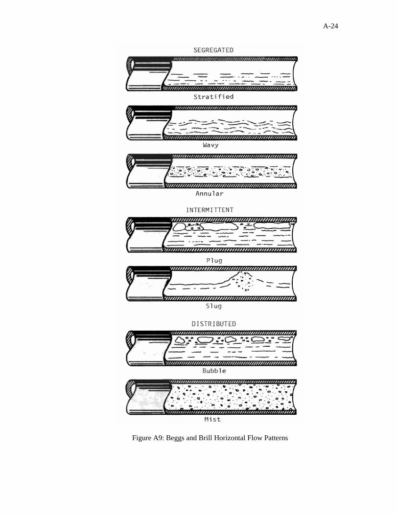
A-24
Figure A9: Beggs and Brill Horizontal Flow Patterns
A-25
(segregated, intermittent and distributed) with a correction for inclination angle of pipe.
A two-phase friction factor is calculated independent of flow regime but depends on
liquid holdup. Hold up factor is calculated as a function of horizontal hold up. Flow
patterns also were determined using dimensionless groups.
Figure C10 shows a normalized friction factor as a function of liquid holdup and input
liquid content.
cFR
bL
L NaH λ
=)0(
Where: )0(LH is the holdup, which would exist at the same conditions in a
horizontal pipe. a, b, and c are determined for each flow pattern from Table A1, with
the restriction that
LLH λ≥)0( .
No slip holdup:
m
sLL V
V=λ
Froude number can be obtained by the equation
gdV
N mFR
2
=
The dimensionless group of Beggs and Brill correlation can be stated as;
302.01 316 LL λ=
4684.22 0009252.0 −= LL λ
4516.13 10.0 −= LL λ
738.64 50.0 −= LL λ
In order to correct the holdup for the effect of pipe inclination ( )φ ; the
following equation is used
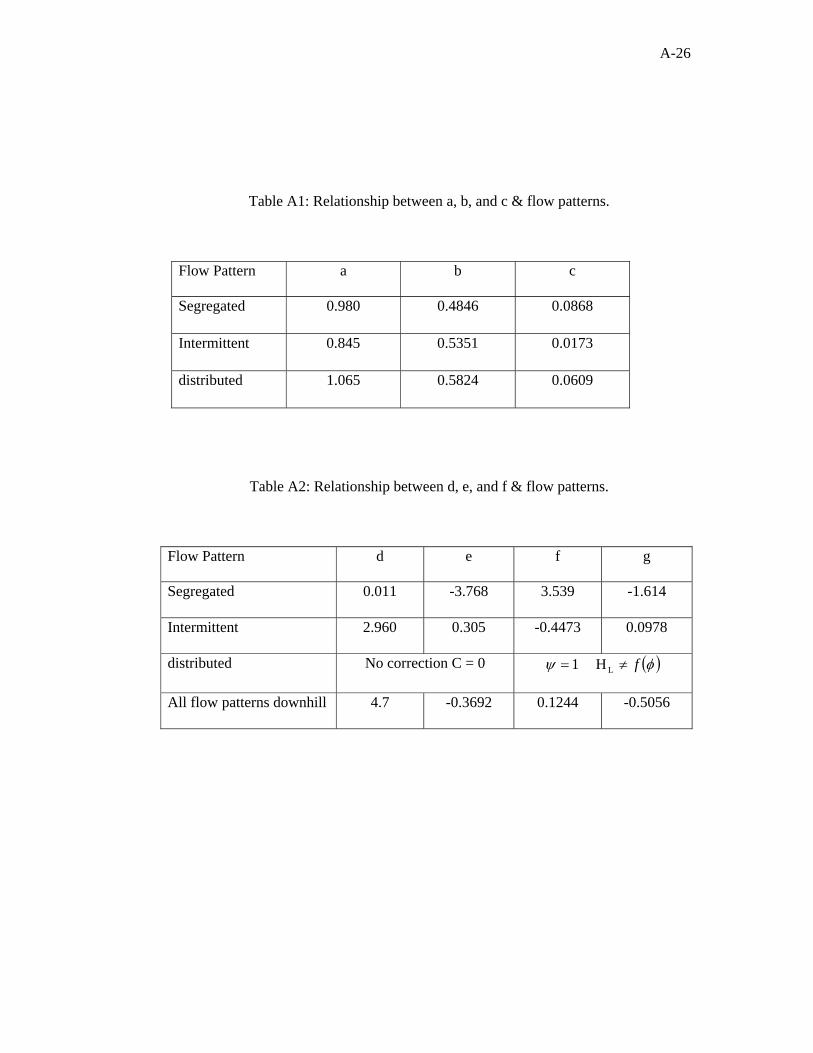
A-26
Table A1: Relationship between a, b, and c & flow patterns.
Flow Pattern a b c
Segregated 0.980 0.4846 0.0868
Intermittent 0.845 0.5351 0.0173
distributed 1.065 0.5824 0.0609
Table A2: Relationship between d, e, and f & flow patterns.
Flow Pattern d e f g
Segregated 0.011 -3.768 3.539 -1.614
Intermittent 2.960 0.305 -0.4473 0.0978
distributed No correction C = 0 ( )φψ f≠= LH 1
All flow patterns downhill 4.7 -0.3692 0.1244 -0.5056
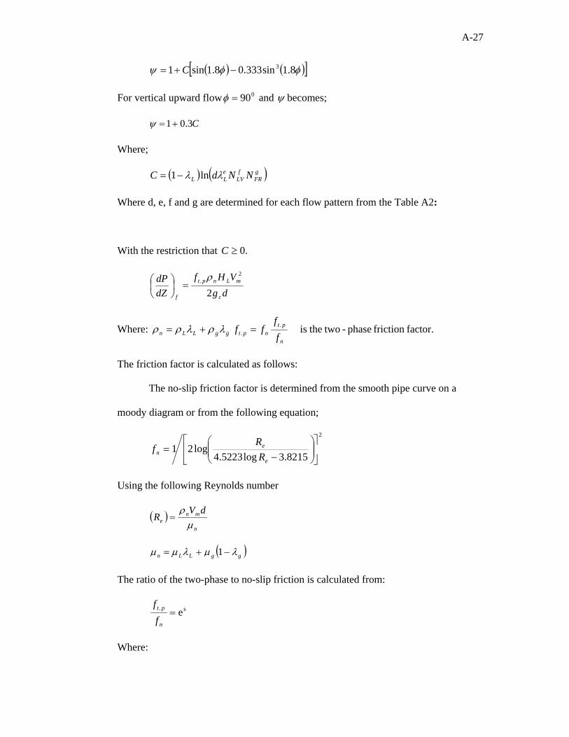
A-27
( ) ( )[ ]φφψ 8.1sin333.08.1sin1 3−+= C
For vertical upward flow 090=φ and ψ becomes;
C3.01+=ψ
Where;
( ) ( )gFR
fLV
eLL NNdC λλ ln1−=
Where d, e, f and g are determined for each flow pattern from the Table A2:
With the restriction that .0≥C
dgVHf
dZdP
c
mLnpt
f 2
2. ρ=⎟
⎠⎞
⎜⎝⎛
Where: ggLLn λρλρρ += factor.friction phase- two theis ..
n
ptnpt f
fff =
The friction factor is calculated as follows:
The no-slip friction factor is determined from the smooth pipe curve on a
moody diagram or from the following equation;
2
8215.3log5223.4log21 ⎥
⎦
⎤⎢⎣
⎡⎟⎟⎠
⎞⎜⎜⎝
⎛−
=e
en R
Rf
Using the following Reynolds number
( )n
mne
dVR
µρ
=
( )ggLLn λµλµµ −+= 1
The ratio of the two-phase to no-slip friction is calculated from:
es. =n
pt
ff
Where:
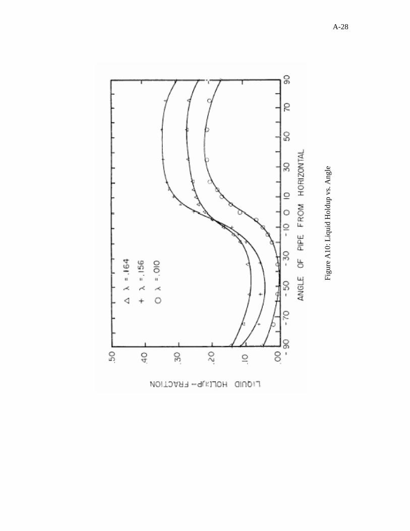
A-28
Figu
re A
10: L
iqui
d H
oldu
p vs
. Ang
le
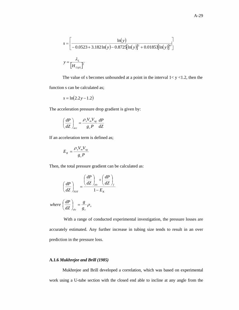
A-29
( )( ) ( )[ ] ( )[ ] ⎥
⎦
⎤⎢⎣
⎡
+−+−= 42 ln01853.0ln8725.0ln182.30523.0
lnyyy
ys
[ ]2)(φ
λ
L
L
Hy =
The value of s becomes unbounded at a point in the interval 1< y <1.2, then the
function s can be calculated as;
( )2.12.2ln −= ys
The acceleration pressure drop gradient is given by:
dZdP
PgVV
dZdP
c
sgms
acc
ρ=⎟
⎠⎞
⎜⎝⎛
If an acceleration term is defined as;
PgVV
Ec
sgmsK
ρ=
Then, the total pressure gradient can be calculated as:
K
felv
TOT EdZdP
dZdP
dZdP
−
⎟⎠⎞
⎜⎝⎛+⎟
⎠⎞
⎜⎝⎛
=⎟⎠⎞
⎜⎝⎛
1
scelv g
gdZdPwhere ρ=⎟
⎠⎞
⎜⎝⎛
With a range of conducted experimental investigation, the pressure losses are
accurately estimated. Any further increase in tubing size tends to result in an over
prediction in the pressure loss.
A.1.6 Mukhrejee and Brill (1985)
Mukhrejee and Brill developed a correlation, which was based on experimental
work using a U-tube section with the closed end able to incline at any angle from the

A-30
horizontal. The correlation developed from their work was tested, with good results, on
data from the Prudhoe Bay and North Sea. This method is applicable to both surface
pipelines and sub-surface tubing, as well. The two-phase fluid flow was divided into four
possible regimes - bubble, slug, stratified and annular-mist.
For the bubble and slug flow regimes, a no-slip friction factor calculated from the
Moody chart is accurate enough. For stratified flow, the friction pressure gradient is
calculated based on a momentum balance equation for either phase assuming a smooth
gas-liquid interface. For annular-mist flow, the friction factor is a function of both the
holdup ratio and the no-slip Moody friction factor. The mixture density is used for
elevation gradient calculation except for the stratified flow where gas density is used.
The acceleration gradient is neglected for the stratified flow.
A.2 Mechanistic Models
The first attempt of generating a mechanistic model was done by Aziz et al.6
who developed a model to calculate multiphase flow parameters and ended up with a
generation of flow pattern map. Rashid Hasan et al.15 addressed multiphase flow from
physical behavior point of view. He nominated four different flow patterns and how to
identify transition between these phases. Besides, void fraction and pressure drop
prediction were estimated in his study. Therefore, he concluded that 90 to 99% of
pressure gradient occurs due to hydrostatic head that is why the need of accurate
estimation of in-situ gas void fraction is much important
A.2.1 Kabir and Hasan (1986)
Kabir and Hasan15 developed a correlation that was based on theoretical
models to predict pressure drop. The hydrodynamic condition was studied carefully
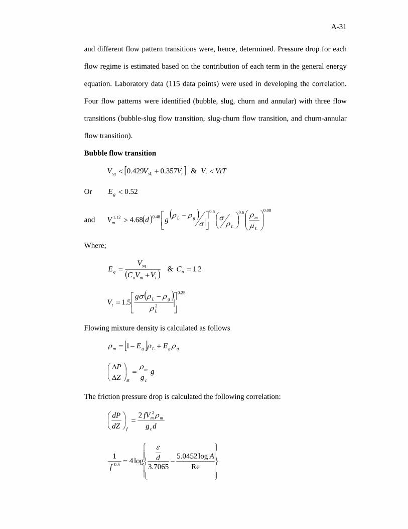
A-31
and different flow pattern transitions were, hence, determined. Pressure drop for each
flow regime is estimated based on the contribution of each term in the general energy
equation. Laboratory data (115 data points) were used in developing the correlation.
Four flow patterns were identified (bubble, slug, churn and annular) with three flow
transitions (bubble-slug flow transition, slug-churn flow transition, and churn-annular
flow transition).
Bubble flow transition
[ ]tsLsg VVV 357.0429.0 +< & VtTVt <
Or 52.0<gE
and ( ) ( ) 08.06.05.048.012.1 68.4 ⎟⎟
⎠
⎞⎜⎜⎝
⎛⎟⎠⎞⎜
⎝⎛
⎥⎦⎤
⎢⎣⎡ −
>L
m
L
gLm gdV
µρ
ρσ
σρρ
Where;
( ) 2.1 & =+
= otmo
sgg C
VVCV
E
( ) 25.0
25.1 ⎥⎦
⎤⎢⎣
⎡ −=
L
gLt
gV
ρρρσ
Flowing mixture density is calculated as follows
[ ] ggLgm EE ρρρ +−= 1
ggZ
P
c
m
st
ρ=⎟
⎠⎞
⎜⎝⎛∆∆
The friction pressure drop is calculated the following correlation:
dgfV
dZdP
c
mm
f
ρ22=⎟
⎠⎞
⎜⎝⎛
⎪⎪⎭
⎪⎪⎬
⎫
⎪⎪⎩
⎪⎪⎨
⎧
−=Re
log0452.57065.3
log415.0
Adf
ε
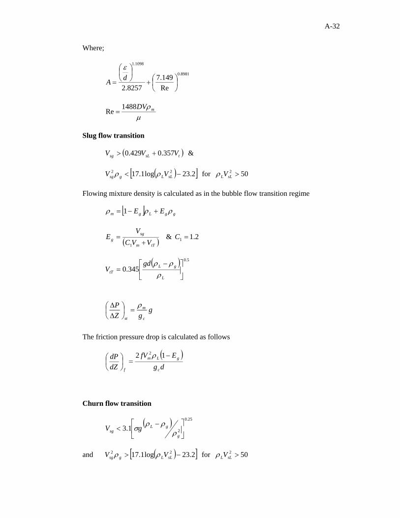
A-32
Where;
8981.0
1098.1
Re149.7
8257.2⎟⎠⎞
⎜⎝⎛+
⎟⎠⎞
⎜⎝⎛
= dA
ε
µρmDV1488
Re =
Slug flow transition
( ) & 357.0429.0 tsLsg VVV +>
( )[ ] 50for 2.23log1.17 222 >−< sLLsLLgsg VVV ρρρ
Flowing mixture density is calculated as in the bubble flow transition regime
[ ] ggLgm EE ρρρ +−= 1
( ) 2.1 & 11
=+
= CVVC
VE
tTm
sgg
( ) 5.0
345.0 ⎥⎦
⎤⎢⎣
⎡ −=
L
gLtT
gdV
ρρρ
The friction pressure drop is calculated as follows
( )dg
EfVdZdP
c
gLm
f
−=⎟
⎠⎞
⎜⎝⎛ 12 2ρ
Churn flow transition
( ) 1.30.25
2 ⎥⎦
⎤⎢⎣
⎡ −<
g
gLsg gV ρ
ρρσ
and ( )[ ] 50for 2.23log1.17 222 >−> sLLsLLgsg VVV ρρρ
ggZ
P
c
m
st
ρ=⎟
⎠⎞
⎜⎝⎛∆∆
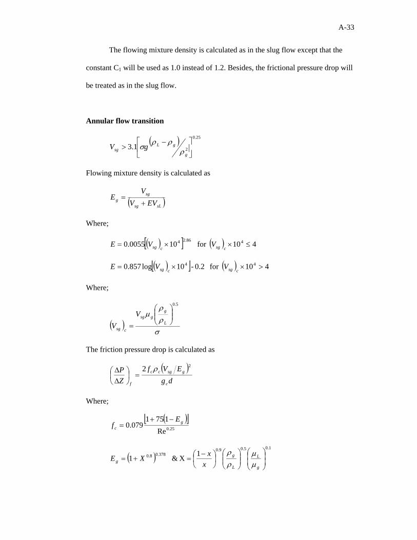
A-33
The flowing mixture density is calculated as in the slug flow except that the
constant C1 will be used as 1.0 instead of 1.2. Besides, the frictional pressure drop will
be treated as in the slug flow.
Annular flow transition
( ) 1.30.25
2 ⎥⎦
⎤⎢⎣
⎡ −>
g
gLsg gV ρ
ρρσ
Flowing mixture density is calculated as
( ) sLsg
sgg EVV
VE
+=
Where;
( )[ ] ( ) 410for 100055.0 486.24 ≤××=csgcsg VVE
( )[ ] ( ) 410for 0.2-10log857.0 44 >××=csgcsg VVE
Where;
( )σρρ
µ5.0
⎟⎟⎠
⎞⎜⎜⎝
⎛
= L
ggsg
csg
VV
The friction pressure drop is calculated as
( )dg
EVfZP
c
gsgcc
f
22 ρ=⎟
⎠⎞
⎜⎝⎛∆∆
Where;
( )[ ]25.0Re
1751079.0 g
c
Ef
−+=
( )1.05.09.0
378.08.0 1X & 1 ⎟⎟⎠
⎞⎜⎜⎝
⎛⎟⎟⎠
⎞⎜⎜⎝
⎛⎟⎠⎞
⎜⎝⎛ −
=+=g
L
L
gg x
xXEµµ
ρρ
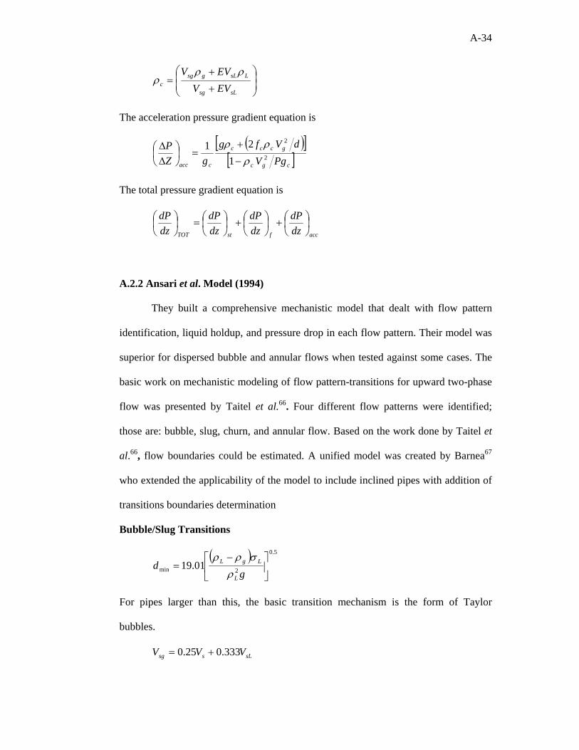
A-34
⎟⎟⎠
⎞⎜⎜⎝
⎛
+
+=
sLsg
LsLgsgc EVV
EVV ρρρ
The acceleration pressure gradient equation is
( )[ ]
[ ]cgc
gccc
cacc PgVdVfg
gZP
2
2
121ρ
ρρ−
+=⎟
⎠⎞
⎜⎝⎛∆∆
The total pressure gradient equation is
accfstTOT dzdP
dzdP
dzdP
dzdP
⎟⎠⎞
⎜⎝⎛+⎟
⎠⎞
⎜⎝⎛+⎟
⎠⎞
⎜⎝⎛=⎟
⎠⎞
⎜⎝⎛
A.2.2 Ansari et al. Model (1994)
They built a comprehensive mechanistic model that dealt with flow pattern
identification, liquid holdup, and pressure drop in each flow pattern. Their model was
superior for dispersed bubble and annular flows when tested against some cases. The
basic work on mechanistic modeling of flow pattern-transitions for upward two-phase
flow was presented by Taitel et al.66. Four different flow patterns were identified;
those are: bubble, slug, churn, and annular flow. Based on the work done by Taitel et
al.66, flow boundaries could be estimated. A unified model was created by Barnea67
who extended the applicability of the model to include inclined pipes with addition of
transitions boundaries determination
Bubble/Slug Transitions
( ) 5.0
2min 01.19 ⎥⎦
⎤⎢⎣
⎡ −=
gd
L
LgL
ρσρρ
For pipes larger than this, the basic transition mechanism is the form of Taylor
bubbles.
sLssg VVV 333.025.0 +=
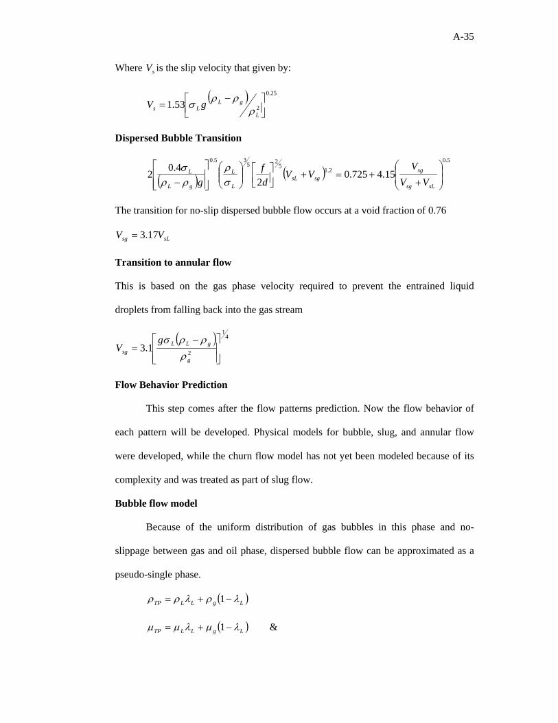
A-35
Where sV is the slip velocity that given by:
( ) 53.10.25
2 ⎥⎦⎤
⎢⎣⎡ −
=L
gLLs gV ρ
ρρσ
Dispersed Bubble Transition
( ) ( )5.0
2.15
2535.0
15.4725.02
4.02 ⎟⎟⎠
⎞⎜⎜⎝
⎛
++=+⎥⎦
⎤⎢⎣⎡
⎟⎟⎠
⎞⎜⎜⎝
⎛
⎥⎥⎦
⎤
⎢⎢⎣
⎡
− sLsg
sgsgsL
L
L
gL
L
VVV
VVdf
g σρ
ρρσ
The transition for no-slip dispersed bubble flow occurs at a void fraction of 0.76
sLsg VV 17.3=
Transition to annular flow
This is based on the gas phase velocity required to prevent the entrained liquid
droplets from falling back into the gas stream
( ) 41
21.3⎥⎥⎦
⎤
⎢⎢⎣
⎡ −=
g
gLLsg
gV
ρρρσ
Flow Behavior Prediction
This step comes after the flow patterns prediction. Now the flow behavior of
each pattern will be developed. Physical models for bubble, slug, and annular flow
were developed, while the churn flow model has not yet been modeled because of its
complexity and was treated as part of slug flow.
Bubble flow model
Because of the uniform distribution of gas bubbles in this phase and no-
slippage between gas and oil phase, dispersed bubble flow can be approximated as a
pseudo-single phase.
( )LgLLTP λρλρρ −+= 1
( )LgLLTP λµλµµ −+= 1 &
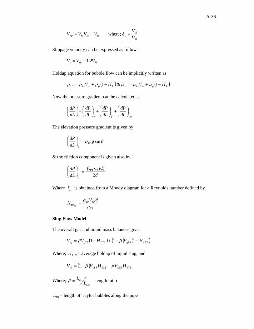
A-36
M
sLsgsLMTP V
VVVVV =+= L re; whe λ
Slippage velocity can be expressed as follows
Msgs VVV 2.1−=
Holdup equation for bubble flow can be implicitly written as
( ) ( )LgLLTPLgLLTP HHHH −+=−+= 1&1 µµµρρρ
Now the pressure gradient can be calculated as
accfe dLdP
dLdP
dLdP
dLdP
⎟⎠⎞
⎜⎝⎛+⎟
⎠⎞
⎜⎝⎛+⎟
⎠⎞
⎜⎝⎛=⎟
⎠⎞
⎜⎝⎛
The elevation pressure gradient is given by
θρ singdLdP
TPe
=⎟⎠⎞
⎜⎝⎛
& the friction component is given also by
dVf
dLdP TPTPTP
f 2
2ρ=⎟
⎠⎞
⎜⎝⎛
Where TPf is obtained from a Moody diagram for a Reynolds number defined by
TP
TPTP dVN
TP µρ
=Re
Slug Flow Model
The overall gas and liquid mass balances gives
( ) ( ) ( )LLSgLSLTBgTBsg HVHVV −−+−= 111 ββ
Where; LLSH = average holdup of liquid slug, and
( ) LTBLTBLLSLLSsL HVHVV ββ −−= 1
Where; SU
TBL
L=β = length ratio
TBL = length of Taylor bubbles along the pipe
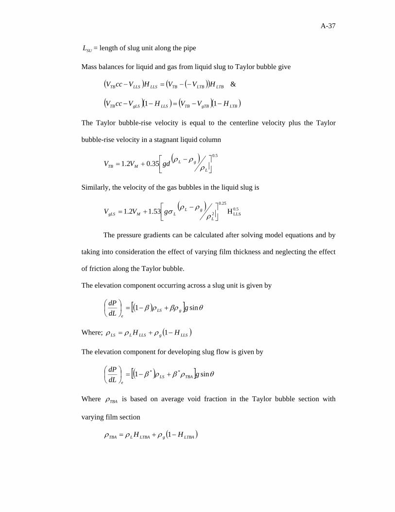
A-37
SUL = length of slug unit along the pipe
Mass balances for liquid and gas from liquid slug to Taylor bubble give
( ) ( )( ) LTBLTBTBLLSLLSTB HVVHVccV −−=− &
( )( ) ( )( )LTBgTBTBLLSgLSTB HVVHVccV −−=−− 11
The Taylor bubble-rise velocity is equal to the centerline velocity plus the Taylor
bubble-rise velocity in a stagnant liquid column
( ) 35.02.10.5
⎥⎦⎤
⎢⎣⎡ −
+=L
gLMTB gdVV ρ
ρρ
Similarly, the velocity of the gas bubbles in the liquid slug is
( ) H53.12.1 0.5LLS
0.25
2 ⎥⎦⎤
⎢⎣⎡ −
+=L
gLLMgLS gVV ρ
ρρσ
The pressure gradients can be calculated after solving model equations and by
taking into consideration the effect of varying film thickness and neglecting the effect
of friction along the Taylor bubble.
The elevation component occurring across a slug unit is given by
( )[ ] θβρρβ sin1 gdLdP
gLSe
+−=⎟⎠⎞
⎜⎝⎛
Where; ( )LLSgLLSLLS HH −+= 1ρρρ
The elevation component for developing slug flow is given by
( )[ ] θρβρβ sin1 ** gdLdP
TBALSe
+−=⎟⎠⎞
⎜⎝⎛
Where TBAρ is based on average void fraction in the Taylor bubble section with
varying film section
( )LTBAgLTBALTBA HH −+= 1ρρρ
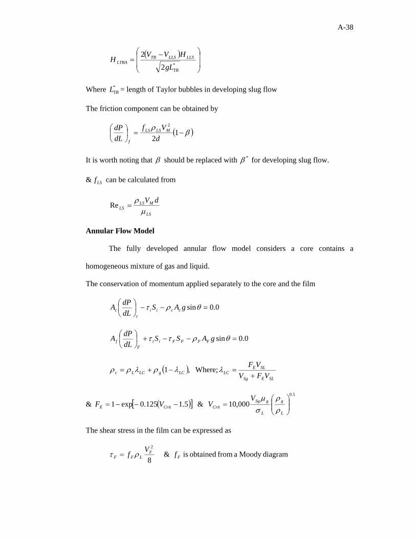
A-38
( )⎟⎟
⎠
⎞
⎜⎜
⎝
⎛ −=
*2
2
TB
LLSLLSTBLTBA
gL
HVVH
Where *TBL = length of Taylor bubbles in developing slug flow
The friction component can be obtained by
( )βρ−=⎟
⎠⎞
⎜⎝⎛ 1
2
2
dVf
dLdP MLSLS
f
It is worth noting that β should be replaced with *β for developing slug flow.
& LSf can be calculated from
LS
MLSLS
dVµ
ρ=Re
Annular Flow Model
The fully developed annular flow model considers a core contains a
homogeneous mixture of gas and liquid.
The conservation of momentum applied separately to the core and the film
0.0sin =−−⎟⎠⎞
⎜⎝⎛ θρτ gAS
dLdPA ccii
cc
0.0sin =−−+⎟⎠⎞
⎜⎝⎛ θρττ gASS
dLdPA FFFFii
Ff
( )SLESg
SLELCLCgLCLc VFV
VF+
=−+= λλρλρρ Where;,1
& ( )[ ]5.0
000,10 & 5.1125.0exp1 ⎟⎟⎠
⎞⎜⎜⎝
⎛=−−−=
L
g
L
gSgCritCritE
VVVF
ρρ
σµ
The shear stress in the film can be expressed as
diagramMoody a from obtained is & 8
2
FF
LFF fVf ρτ =
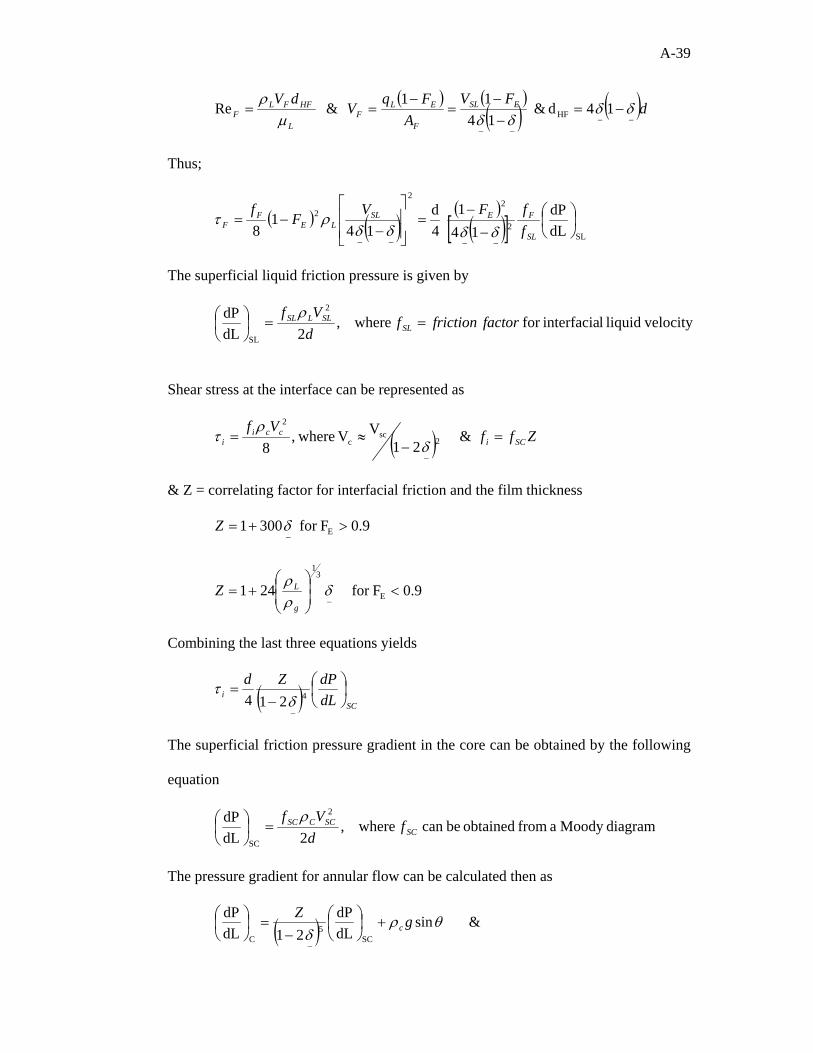
A-39
( ) ( )( ) ( )dFV
AFq
VdV ESL
F
ELF
L
HFFLF −−
−−
−=−−
=−
== δδδδµ
ρ14d&
1411
& Re HF
Thus;
( ) ( )( )( )[ ]
dLdP
141
4d
141
8 SL2
22
2 ⎟⎠⎞
⎜⎝⎛
−−
=⎥⎥⎦
⎤
⎢⎢⎣
⎡
−−=
−−−− SL
FESLLE
FF f
fFVF
fδδδδ
ρτ
The superficial liquid friction pressure is given by
velocityliquid linterfaciafor where,2dL
dP 2
SL
factorfrictionfdVf
SLSLLSL ==⎟
⎠⎞
⎜⎝⎛ ρ
Shear stress at the interface can be represented as
( ) ZffVf
SCicci
i =−
≈=−
& 21
V V where,8 2
scc
2
δρ
τ
& Z = correlating factor for interfacial friction and the film thickness
9.0Ffor 3001 E >+=−δZ
9.0Ffor 241 E
31
<⎟⎟⎠
⎞⎜⎜⎝
⎛+=
−δ
ρρ
g
LZ
Combining the last three equations yields
( ) SCi dL
dPZd⎟⎠⎞
⎜⎝⎛
−=
−
4214 δτ
The superficial friction pressure gradient in the core can be obtained by the following
equation
diagramMoody a from obtained becan where,2dL
dP 2
SCSC
SCCSC fd
Vf ρ=⎟
⎠⎞
⎜⎝⎛
The pressure gradient for annular flow can be calculated then as
( ) & sindLdP
21dLdP
SC5
C
θρδ
gZc+⎟
⎠⎞
⎜⎝⎛
−=⎟
⎠⎞
⎜⎝⎛
−
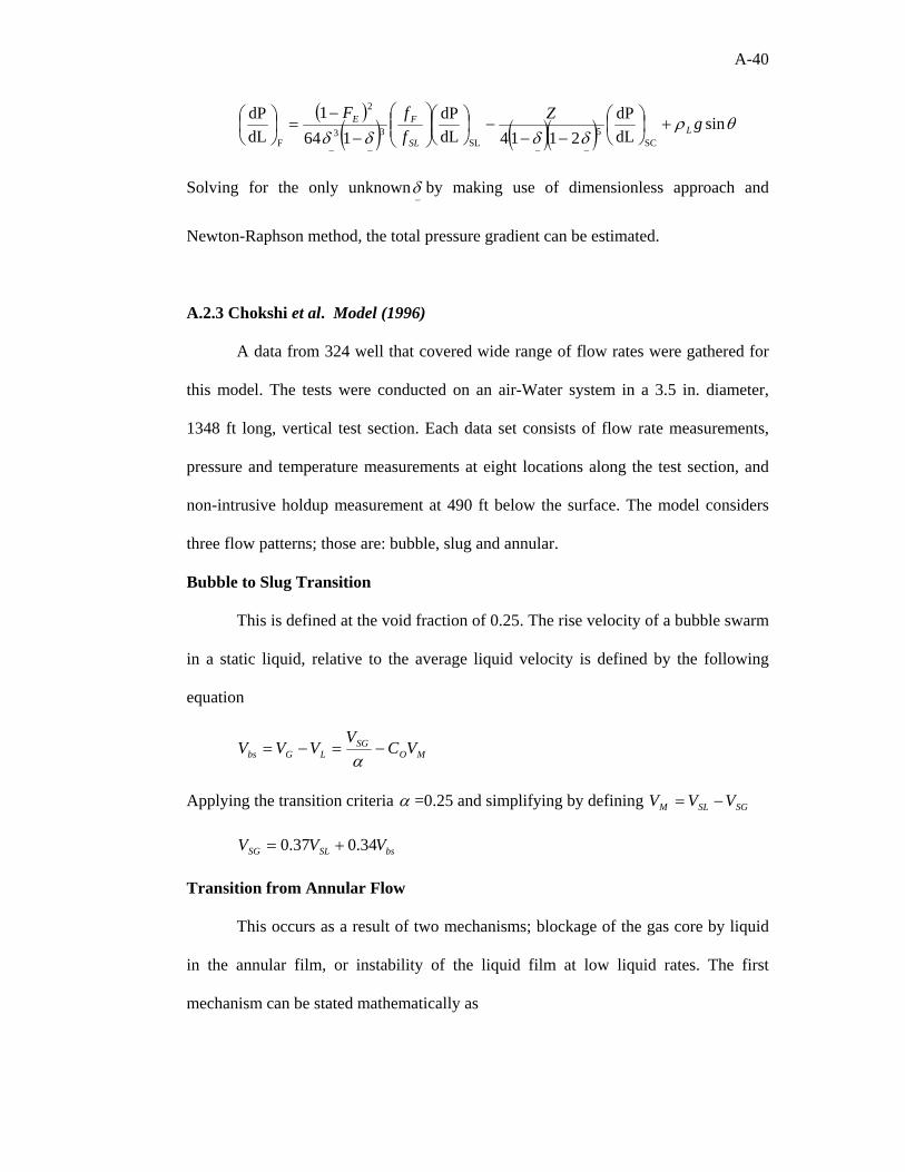
A-40
( )( ) ( )( ) sin
dLdP
2114dLdP
1641
dLdP
SC5
SL33
2
F
θρδδδδ
gZffF
LSL
FE +⎟⎠⎞
⎜⎝⎛
−−−⎟
⎠⎞
⎜⎝⎛⎟⎟⎠
⎞⎜⎜⎝
⎛
−−
=⎟⎠⎞
⎜⎝⎛
−−−−
Solving for the only unknown−δ by making use of dimensionless approach and
Newton-Raphson method, the total pressure gradient can be estimated.
A.2.3 Chokshi et al. Model (1996)
A data from 324 well that covered wide range of flow rates were gathered for
this model. The tests were conducted on an air-Water system in a 3.5 in. diameter,
1348 ft long, vertical test section. Each data set consists of flow rate measurements,
pressure and temperature measurements at eight locations along the test section, and
non-intrusive holdup measurement at 490 ft below the surface. The model considers
three flow patterns; those are: bubble, slug and annular.
Bubble to Slug Transition
This is defined at the void fraction of 0.25. The rise velocity of a bubble swarm
in a static liquid, relative to the average liquid velocity is defined by the following
equation
MOSG
LGbs VCV
VVV −=−=α
Applying the transition criteria α =0.25 and simplifying by defining SGSLM VVV −=
bsSLSG VVV 34.037.0 +=
Transition from Annular Flow
This occurs as a result of two mechanisms; blockage of the gas core by liquid
in the annular film, or instability of the liquid film at low liquid rates. The first
mechanism can be stated mathematically as
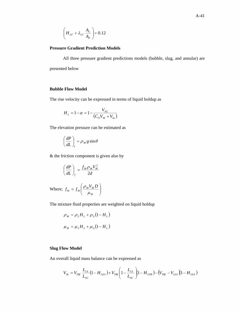
A-41
12.0=⎟⎟⎠
⎞⎜⎜⎝
⎛+
P
CLCLF A
AH λ
Pressure Gradient Prediction Models
All three pressure gradient predictions models (bubble, slug, and annular) are
presented below
Bubble Flow Model
The rise velocity can be expressed in terms of liquid holdup as
( )bsMO
SGL VVC
VH
+−=−= 11 α
The elevation pressure can be estimated as
θρ singdLdP
Me
=⎟⎠⎞
⎜⎝⎛
& the friction component is given also by
dVf
dLdP MMM
f 2
2ρ=⎟
⎠⎞
⎜⎝⎛
Where; ⎟⎟⎠
⎞⎜⎜⎝
⎛=
M
MMMM
DVffµ
ρ
The mixture fluid properties are weighted on liquid holdup
( )LGLLM HH −+= 1ρρρ
( )LGLLM HH −+= 1µµµ
Slug Flow Model
An overall liquid mass balance can be expressed as
( ) ( ) ( )( )GLSLLSTBfGTBSU
LSTBfGLS
SU
LSTBfSL HVVH
LL
VHLL
VV −−−−⎟⎟⎠
⎞⎜⎜⎝
⎛−+−= 1111
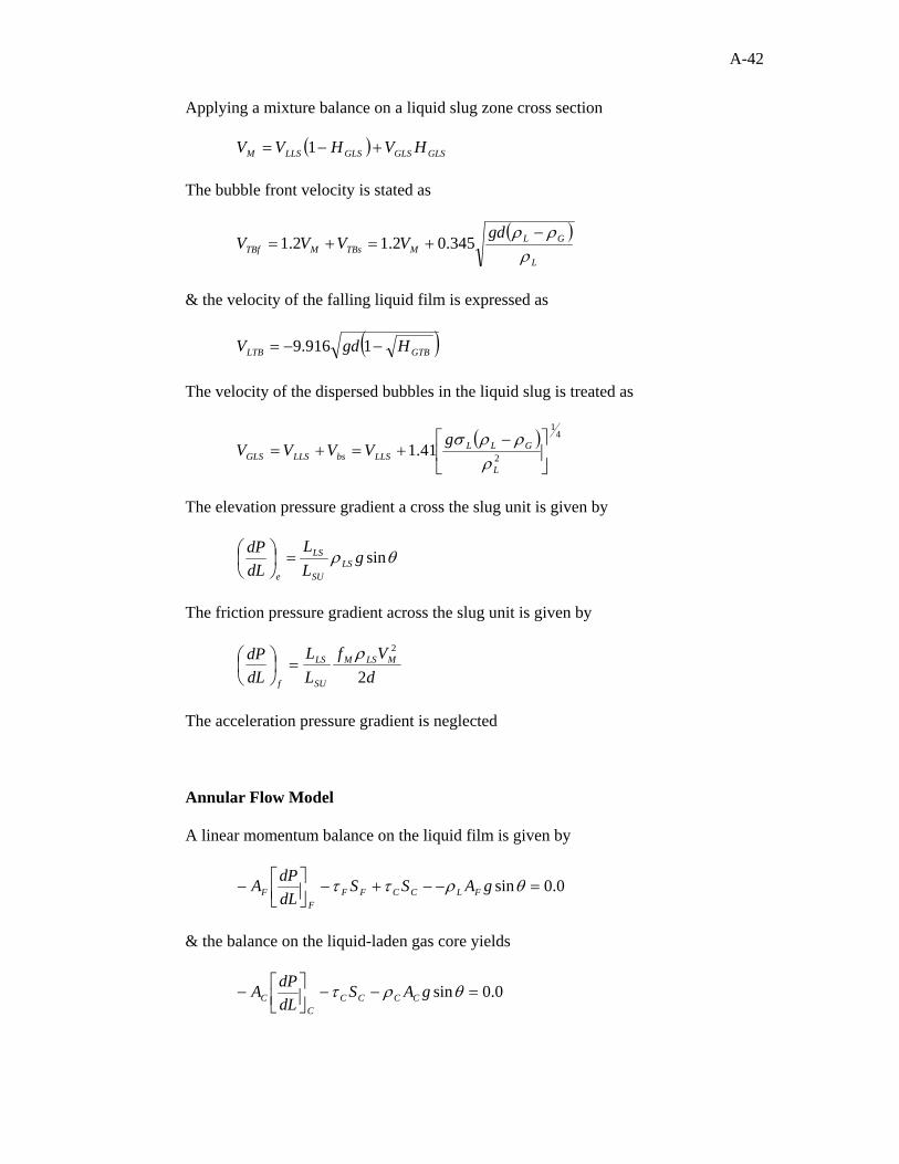
A-42
Applying a mixture balance on a liquid slug zone cross section
( ) GLSGLSGLSLLSM HVHVV +−= 1
The bubble front velocity is stated as
( )L
GLMTBsMTBf
gdVVVV
ρρρ −
+=+= 345.02.12.1
& the velocity of the falling liquid film is expressed as
( )GTBLTB HgdV −−= 1916.9
The velocity of the dispersed bubbles in the liquid slug is treated as
( ) 41
241.1 ⎥⎦
⎤⎢⎣
⎡ −+=+=
L
GLLLLSbsLLSGLS
gVVVV
ρρρσ
The elevation pressure gradient a cross the slug unit is given by
θρ singLL
dLdP
LSSU
LS
e
=⎟⎠⎞
⎜⎝⎛
The friction pressure gradient across the slug unit is given by
dVf
LL
dLdP MLSM
SU
LS
f 2
2ρ=⎟
⎠⎞
⎜⎝⎛
The acceleration pressure gradient is neglected
Annular Flow Model
A linear momentum balance on the liquid film is given by
0.0sin =−−+−⎥⎦⎤
⎢⎣⎡− θρττ gASS
dLdPA FLCCFF
FF
& the balance on the liquid-laden gas core yields
0.0sin =−−⎥⎦⎤
⎢⎣⎡− θρτ gAS
dLdPA CCCC
CC
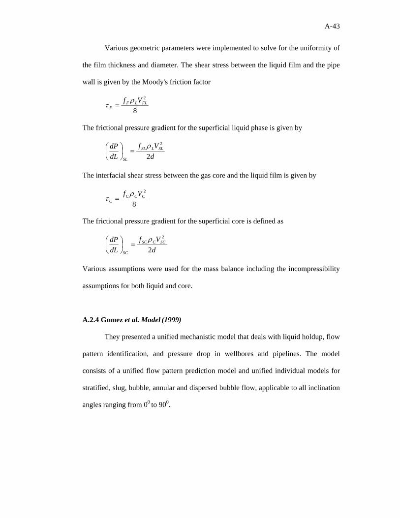
A-43
Various geometric parameters were implemented to solve for the uniformity of
the film thickness and diameter. The shear stress between the liquid film and the pipe
wall is given by the Moody's friction factor
8
2FLLF
FVf ρ
τ =
The frictional pressure gradient for the superficial liquid phase is given by
dVf
dLdP SLLSL
SL 2
2ρ=⎟
⎠⎞
⎜⎝⎛
The interfacial shear stress between the gas core and the liquid film is given by
8
2CCC
CVf ρ
τ =
The frictional pressure gradient for the superficial core is defined as
dVf
dLdP SCCSC
SC 2
2ρ=⎟
⎠⎞
⎜⎝⎛
Various assumptions were used for the mass balance including the incompressibility
assumptions for both liquid and core.
A.2.4 Gomez et al. Model (1999)
They presented a unified mechanistic model that deals with liquid holdup, flow
pattern identification, and pressure drop in wellbores and pipelines. The model
consists of a unified flow pattern prediction model and unified individual models for
stratified, slug, bubble, annular and dispersed bubble flow, applicable to all inclination
angles ranging from 00 to 900.
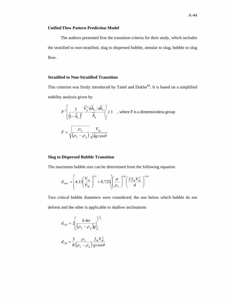
A-44
Unified Flow Pattern Prediction Model
The authors presented first the transition criteria for their study, which includes
the stratified to non-stratified, slug to dispersed bubble, annular to slug, bubble to slug
flow.
Stratified to Non-Stratified Transition
This criterion was firstly introduced by Taitel and Dukler66. It is based on a simplified
stability analysis given by
( ) group essdimensionl a is F where, 1~
~~~
~1
1 2
22 ≥
⎥⎥⎦
⎤
⎢⎢⎣
⎡
− g
LLg
LA
hdAdV
hF
( ) θρρρ
cosdg
VF sg
gL
g
−=
Slug to Dispersed Bubble Transition
The maximum bubble size can be determined from the following equation
4.036.05.0
max2
725.015.4−
⎟⎟⎠
⎞⎜⎜⎝
⎛⎟⎟⎠
⎞⎜⎜⎝
⎛
⎥⎥⎦
⎤
⎢⎢⎣
⎡+⎟⎟
⎠
⎞⎜⎜⎝
⎛=
dVf
VV
d MM
LM
sg
ρσ
Two critical bubble diameters were considered; the one below which bubble do not
deform and the other is applicable to shallow inclinations
( )2
1
4.02⎥⎥⎦
⎤
⎢⎢⎣
⎡
−=
gd
gLCD ρρ
σ
( ) θρρρ
cos83 2
gVfd MM
gL
LCB −
=
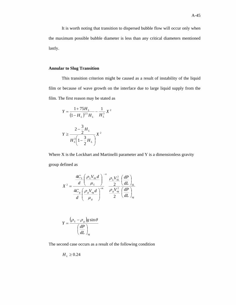
A-45
It is worth noting that transition to dispersed bubble flow will occur only when
the maximum possible bubble diameter is less than any critical diameters mentioned
lastly.
Annular to Slug Transition
This transition criterion might be caused as a result of instability of the liquid
film or because of wave growth on the interface due to large liquid supply from the
film. The first reason may be stated as
( )2
35.2
11
751X
HHHH
YLLL
L −−+
=
2
3
231
232
XHH
HY
LL
L
⎟⎠⎞
⎜⎝⎛ −
−≥
Where X is the Lockhart and Martinelli parameter and Y is a dimensionless gravity
group defined as
sg
SL
sgg
SLL
n
m
g
sggg
L
SLLL
dLdPdLdP
V
V
dVdC
dVdC
X⎟⎠⎞
⎜⎝⎛
⎟⎠⎞
⎜⎝⎛
⎟⎟⎠
⎞⎜⎜⎝
⎛
⎟⎟⎠
⎞⎜⎜⎝
⎛
=
−
−
2
24
4
2
2
2
ρ
ρ
µρ
µρ
( )
sg
gL
dLdP
gY
⎟⎠⎞
⎜⎝⎛
−=
θρρ sin
The second case occurs as a result of the following condition
24.0≥LH
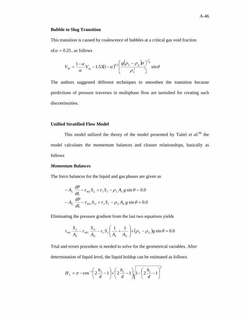
A-46
Bubble to Slug Transition
This transition is caused by coalescence of bubbles at a critical gas void fraction
of 25.0=α , as follows
( ) ( )θ
ρσρρ
ααα sin153.11 4
1
25.0
⎥⎦
⎤⎢⎣
⎡ −−−
−=
L
gLsgSL
gVV
The authors suggested different techniques to smoothen the transition because
predictions of pressure traverses in multiphase flow are tarnished for creating such
discontinuities.
Unified Stratified Flow Model
This model utilized the theory of the model presented by Taitel et al.66 the
model calculates the momentum balances and closure relationships, basically as
follows
Momentum Balances
The force balances for the liquid and gas phases are given as
0.0sin
0.0sin
=−+−−
=−+−−
θρττ
θρττ
gASSdLdPA
gASSdLdPA
GGIIGWGG
LLIILWLL
Eliminating the pressure gradient from the last two equations yields
( ) 0.0sin11=−+⎟⎟
⎠
⎞⎜⎜⎝
⎛+−− θρρτττ g
AAS
AS
AS
GLGL
IIG
GWG
L
LWL
Trial and errors procedure is needed to solve for the geometrical variables. After
determination of liquid level, the liquid holdup can be estimated as follows
21 1211212cos ⎟
⎠
⎞⎜⎝
⎛ −−⎟⎠
⎞⎜⎝
⎛ −+⎟⎠
⎞⎜⎝
⎛ −−= −
dh
dh
dh
H LLLL π
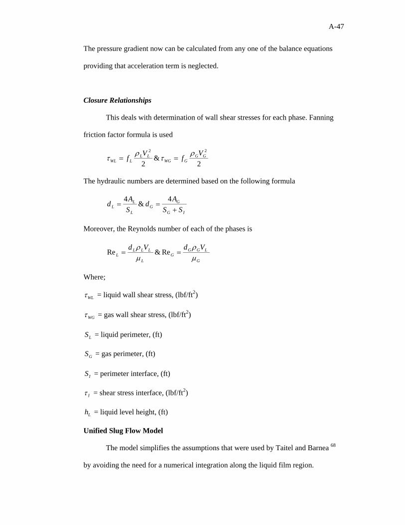
A-47
The pressure gradient now can be calculated from any one of the balance equations
providing that acceleration term is neglected.
Closure Relationships
This deals with determination of wall shear stresses for each phase. Fanning
friction factor formula is used
2&
2
22GG
GWGLL
LWLV
fVfρ
τρ
τ ==
The hydraulic numbers are determined based on the following formula
IG
GG
L
LL SS
Ad
SA
d+
==4
&4
Moreover, the Reynolds number of each of the phases is
G
LGGG
L
LLLL
VdVdµρ
µρ
== Re&Re
Where;
WLτ = liquid wall shear stress, (lbf/ft2)
WGτ = gas wall shear stress, (lbf/ft2)
LS = liquid perimeter, (ft)
GS = gas perimeter, (ft)
IS = perimeter interface, (ft)
Iτ = shear stress interface, (lbf/ft2)
Lh = liquid level height, (ft)
Unified Slug Flow Model
The model simplifies the assumptions that were used by Taitel and Barnea 68
by avoiding the need for a numerical integration along the liquid film region.
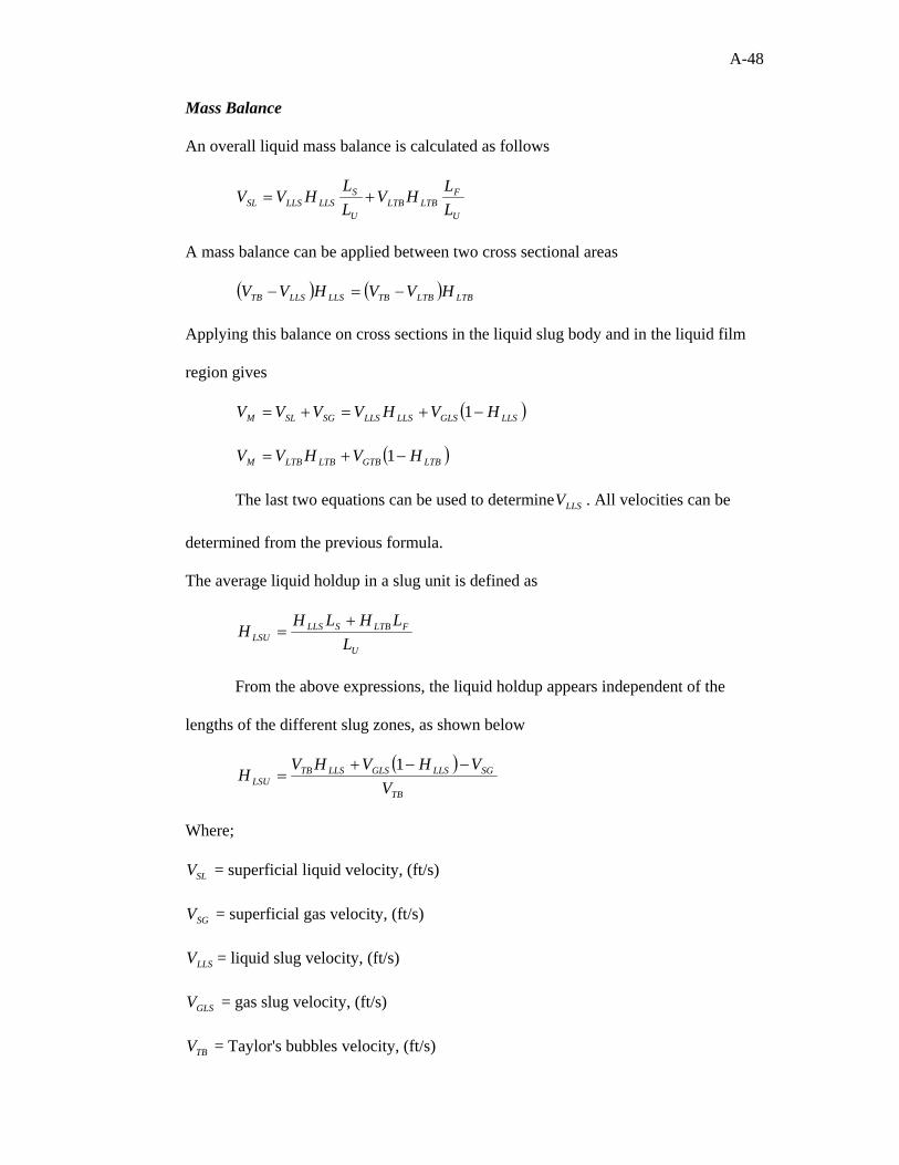
A-48
Mass Balance
An overall liquid mass balance is calculated as follows
U
FLTBLTB
U
SLLSLLSSL L
LHVLL
HVV +=
A mass balance can be applied between two cross sectional areas
( ) ( ) LTBLTBTBLLSLLSTB HVVHVV −=−
Applying this balance on cross sections in the liquid slug body and in the liquid film
region gives
( )LLSGLSLLSLLSSGSLM HVHVVVV −+=+= 1
( )LTBGTBLTBLTBM HVHVV −+= 1
The last two equations can be used to determine LLSV . All velocities can be
determined from the previous formula.
The average liquid holdup in a slug unit is defined as
U
FLTBSLLSLSU L
LHLHH
+=
From the above expressions, the liquid holdup appears independent of the
lengths of the different slug zones, as shown below
( )TB
SGLLSGLSLLSTBLSU V
VHVHVH
−−+=
1
Where;
SLV = superficial liquid velocity, (ft/s)
SGV = superficial gas velocity, (ft/s)
LLSV = liquid slug velocity, (ft/s)
GLSV = gas slug velocity, (ft/s)
TBV = Taylor's bubbles velocity, (ft/s)
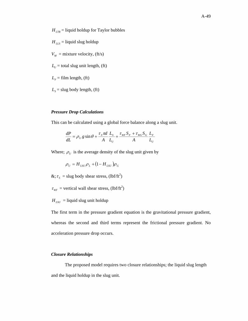
A-49
LTBH = liquid holdup for Taylor bubbles
LLSH = liquid slug holdup
MV = mixture velocity, (ft/s)
UL = total slug unit length, (ft)
FL = film length, (ft)
SL = slug body length, (ft)
Pressure Drop Calculations
This can be calculated using a global force balance along a slug unit.
U
FGWGFWF
U
SSU L
LA
SSLL
Ad
gdLdP ττπτ
θρ+
++= sin
Where; Uρ is the average density of the slug unit given by
( ) GLSULLSUU HH ρρρ −+= 1
&; Sτ = slug body shear stress, (lbf/ft2)
WFτ = vertical wall shear stress, (lbf/ft2)
LSUH = liquid slug unit holdup
The first term in the pressure gradient equation is the gravitational pressure gradient,
whereas the second and third terms represent the frictional pressure gradient. No
acceleration pressure drop occurs.
Closure Relationships
The proposed model requires two closure relationships; the liquid slug length
and the liquid holdup in the slug unit.
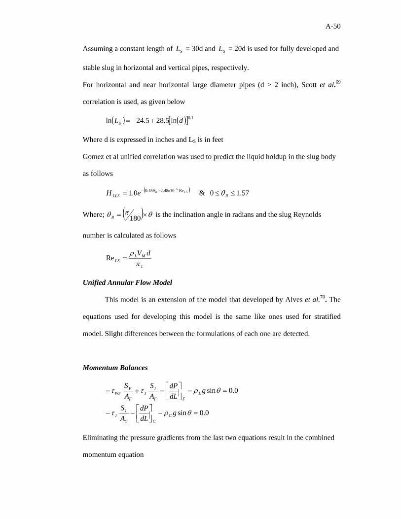
A-50
Assuming a constant length of SL = 30d and SL = 20d is used for fully developed and
stable slug in horizontal and vertical pipes, respectively.
For horizontal and near horizontal large diameter pipes (d > 2 inch), Scott et al.69
correlation is used, as given below
( ) ( )[ ] 1.0ln5.285.24ln dLS +−=
Where d is expressed in inches and LS is in feet
Gomez et al unified correlation was used to predict the liquid holdup in the slug body
as follows
( ) 57.10 & 0.1 Re1048.245.0 6
≤≤=−×+−
RLLSLSReH θθ
Where; ( ) θπθ ×= 180R is the inclination angle in radians and the slug Reynolds
number is calculated as follows
L
MLLS
dVπ
ρ=Re
Unified Annular Flow Model
This model is an extension of the model that developed by Alves et al.70. The
equations used for developing this model is the same like ones used for stratified
model. Slight differences between the formulations of each one are detected.
Momentum Balances
0.0sin
0.0sin
=−⎥⎦⎤
⎢⎣⎡−−
=−⎥⎦⎤
⎢⎣⎡−+−
θρτ
θρττ
gdLdP
AS
gdLdP
AS
AS
CCC
II
LFF
II
F
FWF
Eliminating the pressure gradients from the last two equations result in the combined
momentum equation
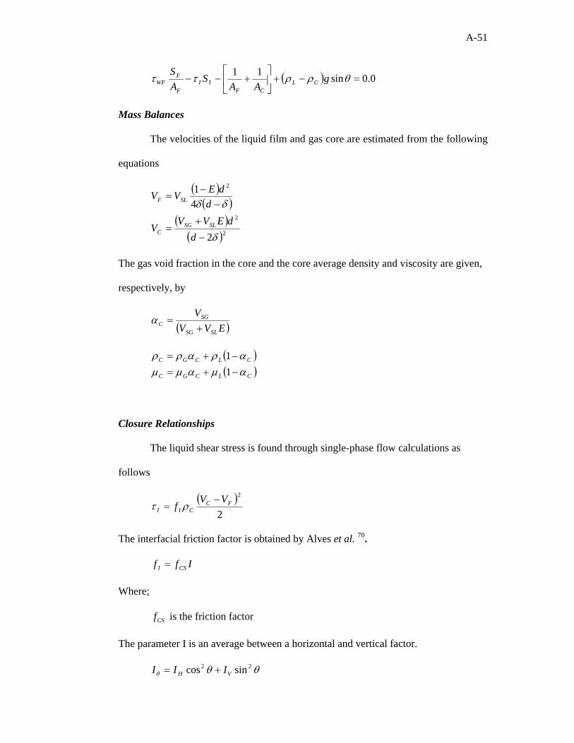
A-51
( ) 0.0sin11=−+⎥
⎦
⎤⎢⎣
⎡+−− θρρττ g
AAS
AS
CLCF
IIF
FWF
Mass Balances
The velocities of the liquid film and gas core are estimated from the following
equations
( )( )
( )( )2
2
2
2
41
δ
δδ
−
+=
−−
=
ddEVV
V
ddEVV
SLSGC
SLF
The gas void fraction in the core and the core average density and viscosity are given,
respectively, by
( )EVVV
SLSG
SGC +=α
( )( )CLCGC
CLCGC
αµαµµαραρρ
−+=−+=
11
Closure Relationships
The liquid shear stress is found through single-phase flow calculations as
follows
( )2
2FC
CIIVV
f−
= ρτ
The interfacial friction factor is obtained by Alves et al. 70.
Iff CSI =
Where;
CSf is the friction factor
The parameter I is an average between a horizontal and vertical factor.
θθθ22 sincos VH III +=
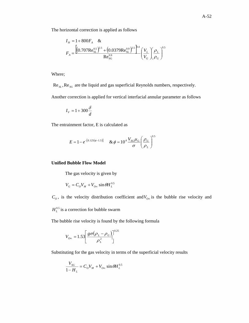
A-52
The horizontal correction is applied as follows
( ) ( )[ ] 5.0
0.9SG
4.05.20.9SL
5.20.5SL
Re0.0379Re0.707Re
& 8001
⎟⎟⎠
⎞⎜⎜⎝
⎛⎟⎟⎠
⎞⎜⎜⎝
⎛+=
+=
G
L
G
LA
AH
VVF
FI
ρρ
Where;
SGSL Re,Re are the liquid and gas superficial Reynolds numbers, respectively.
Another correction is applied for vertical interfacial annular parameter as follows
dIV
δ3001+=
The entrainment factor, E is calculated as
Unified Bubble Flow Model
The gas velocity is given by
5.0sin LOMOG HVVCV θ∞+=
OC , is the velocity distribution coefficient and ∞OV is the bubble rise velocity and
5.0LH is a correction for bubble swarm
The bubble rise velocity is found by the following formula
( ) 25.0
253.1 ⎥⎦
⎤⎢⎣
⎡ −=∞
L
GLO
gV
ρρρσ
Substituting for the gas velocity in terms of the superficial velocity results
5.0sin1 LOMO
L
SG HVVCH
Vθ∞+=
−
( )[ ]5.0
45.1125.0 10& 1 ⎟⎟⎠
⎞⎜⎜⎝
⎛=−= −−
L
GGSGVeEρρ
σµφφ

APPENDIX B
DATA ORGANIZATION
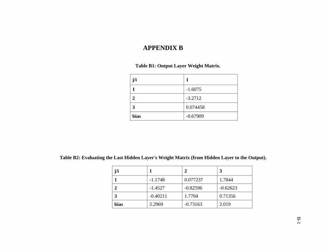
B-1
APPENDIX B
Table B1: Output Layer Weight Matrix.
j/i 1
1 -1.6075
2 -3.2712
3 0.074458
bias -0.67909
Table B2: Evaluating the Last Hidden Layer's Weight Matrix (from Hidden Layer to the Output).
j/i 1 2 3
1 -1.1748 0.077237 1.7844
2 -1.4527 -0.82596 -0.62623
3 -0.40211 1.7704 0.71356
bias 2.2969 -0.73163 2.019
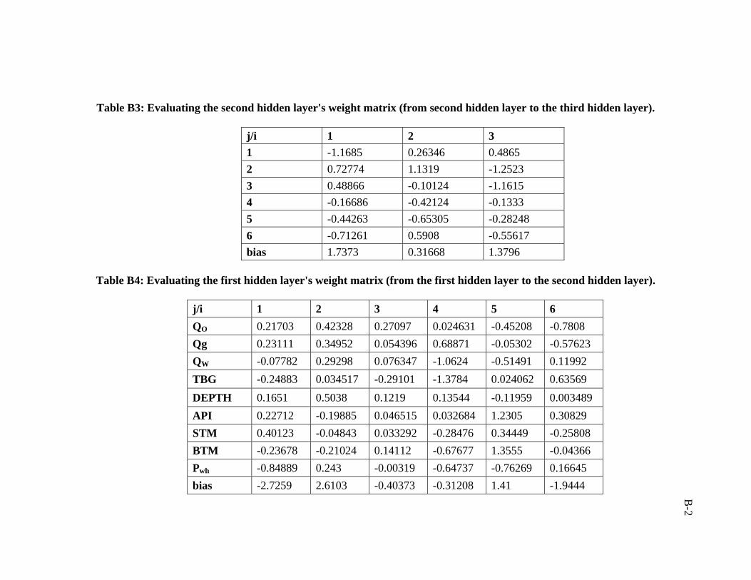
B-2
Table B3: Evaluating the second hidden layer's weight matrix (from second hidden layer to the third hidden layer).
j/i 1 2 3 1 -1.1685 0.26346 0.4865 2 0.72774 1.1319 -1.2523 3 0.48866 -0.10124 -1.1615 4 -0.16686 -0.42124 -0.1333 5 -0.44263 -0.65305 -0.28248 6 -0.71261 0.5908 -0.55617 bias 1.7373 0.31668 1.3796
Table B4: Evaluating the first hidden layer's weight matrix (from the first hidden layer to the second hidden layer).
j/i 1 2 3 4 5 6 QO 0.21703 0.42328 0.27097 0.024631 -0.45208 -0.7808 Qg 0.23111 0.34952 0.054396 0.68871 -0.05302 -0.57623 QW -0.07782 0.29298 0.076347 -1.0624 -0.51491 0.11992 TBG -0.24883 0.034517 -0.29101 -1.3784 0.024062 0.63569 DEPTH 0.1651 0.5038 0.1219 0.13544 -0.11959 0.003489 API 0.22712 -0.19885 0.046515 0.032684 1.2305 0.30829 STM 0.40123 -0.04843 0.033292 -0.28476 0.34449 -0.25808 BTM -0.23678 -0.21024 0.14112 -0.67677 1.3555 -0.04366 Pwh -0.84889 0.243 -0.00319 -0.64737 -0.76269 0.16645 bias -2.7259 2.6103 -0.40373 -0.31208 1.41 -1.9444
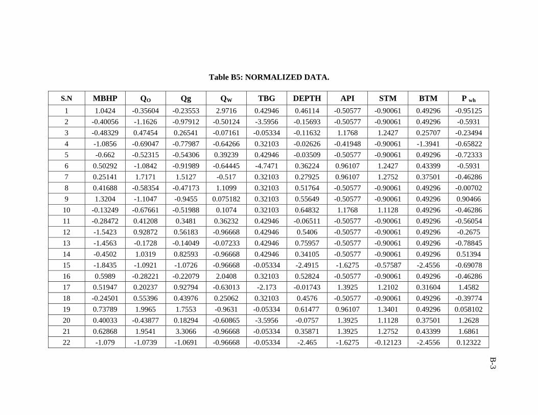
B-3
Table B5: NORMALIZED DATA.
S.N MBHP QO Qg QW TBG DEPTH API STM BTM P wh 1 1.0424 -0.35604 -0.23553 2.9716 0.42946 0.46114 -0.50577 -0.90061 0.49296 -0.95125 2 -0.40056 -1.1626 -0.97912 -0.50124 -3.5956 -0.15693 -0.50577 -0.90061 0.49296 -0.5931 3 -0.48329 0.47454 0.26541 -0.07161 -0.05334 -0.11632 1.1768 1.2427 0.25707 -0.23494 4 -1.0856 -0.69047 -0.77987 -0.64266 0.32103 -0.02626 -0.41948 -0.90061 -1.3941 -0.65822 5 -0.662 -0.52315 -0.54306 0.39239 0.42946 -0.03509 -0.50577 -0.90061 0.49296 -0.72333 6 0.50292 -1.0842 -0.91989 -0.64445 -4.7471 0.36224 0.96107 1.2427 0.43399 -0.5931 7 0.25141 1.7171 1.5127 -0.517 0.32103 0.27925 0.96107 1.2752 0.37501 -0.46286 8 0.41688 -0.58354 -0.47173 1.1099 0.32103 0.51764 -0.50577 -0.90061 0.49296 -0.00702 9 1.3204 -1.1047 -0.9455 0.075182 0.32103 0.55649 -0.50577 -0.90061 0.49296 0.90466
10 -0.13249 -0.67661 -0.51988 0.1074 0.32103 0.64832 1.1768 1.1128 0.49296 -0.46286 11 -0.28472 0.41208 0.3481 0.36232 0.42946 -0.06511 -0.50577 -0.90061 0.49296 -0.56054 12 -1.5423 0.92872 0.56183 -0.96668 0.42946 0.5406 -0.50577 -0.90061 0.49296 -0.2675 13 -1.4563 -0.1728 -0.14049 -0.07233 0.42946 0.75957 -0.50577 -0.90061 0.49296 -0.78845 14 -0.4502 1.0319 0.82593 -0.96668 0.42946 0.34105 -0.50577 -0.90061 0.49296 0.51394 15 -1.8435 -1.0921 -1.0726 -0.96668 -0.05334 -2.4915 -1.6275 -0.57587 -2.4556 -0.69078 16 0.5989 -0.28221 -0.22079 2.0408 0.32103 0.52824 -0.50577 -0.90061 0.49296 -0.46286 17 0.51947 0.20237 0.92794 -0.63013 -2.173 -0.01743 1.3925 1.2102 0.31604 1.4582 18 -0.24501 0.55396 0.43976 0.25062 0.32103 0.4576 -0.50577 -0.90061 0.49296 -0.39774 19 0.73789 1.9965 1.7553 -0.9631 -0.05334 0.61477 0.96107 1.3401 0.49296 0.058102 20 0.40033 -0.43877 0.18294 -0.60865 -3.5956 -0.0757 1.3925 1.1128 0.37501 1.2628 21 0.62868 1.9541 3.3066 -0.96668 -0.05334 0.35871 1.3925 1.2752 0.43399 1.6861 22 -1.079 -1.0739 -1.0691 -0.96668 -0.05334 -2.465 -1.6275 -0.12123 -2.4556 0.12322
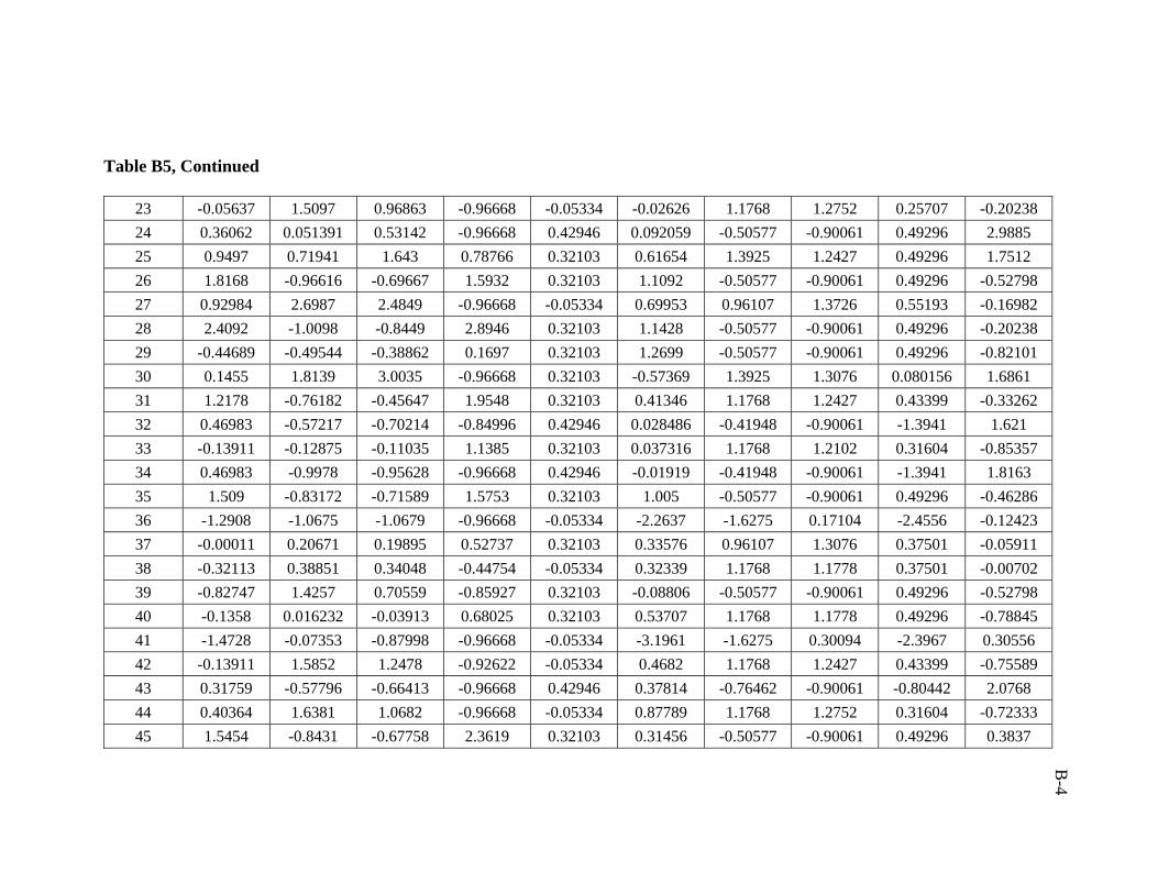
B-4
Table B5, Continued
23 -0.05637 1.5097 0.96863 -0.96668 -0.05334 -0.02626 1.1768 1.2752 0.25707 -0.20238 24 0.36062 0.051391 0.53142 -0.96668 0.42946 0.092059 -0.50577 -0.90061 0.49296 2.9885 25 0.9497 0.71941 1.643 0.78766 0.32103 0.61654 1.3925 1.2427 0.49296 1.7512 26 1.8168 -0.96616 -0.69667 1.5932 0.32103 1.1092 -0.50577 -0.90061 0.49296 -0.52798 27 0.92984 2.6987 2.4849 -0.96668 -0.05334 0.69953 0.96107 1.3726 0.55193 -0.16982 28 2.4092 -1.0098 -0.8449 2.8946 0.32103 1.1428 -0.50577 -0.90061 0.49296 -0.20238 29 -0.44689 -0.49544 -0.38862 0.1697 0.32103 1.2699 -0.50577 -0.90061 0.49296 -0.82101 30 0.1455 1.8139 3.0035 -0.96668 0.32103 -0.57369 1.3925 1.3076 0.080156 1.6861 31 1.2178 -0.76182 -0.45647 1.9548 0.32103 0.41346 1.1768 1.2427 0.43399 -0.33262 32 0.46983 -0.57217 -0.70214 -0.84996 0.42946 0.028486 -0.41948 -0.90061 -1.3941 1.621 33 -0.13911 -0.12875 -0.11035 1.1385 0.32103 0.037316 1.1768 1.2102 0.31604 -0.85357 34 0.46983 -0.9978 -0.95628 -0.96668 0.42946 -0.01919 -0.41948 -0.90061 -1.3941 1.8163 35 1.509 -0.83172 -0.71589 1.5753 0.32103 1.005 -0.50577 -0.90061 0.49296 -0.46286 36 -1.2908 -1.0675 -1.0679 -0.96668 -0.05334 -2.2637 -1.6275 0.17104 -2.4556 -0.12423 37 -0.00011 0.20671 0.19895 0.52737 0.32103 0.33576 0.96107 1.3076 0.37501 -0.05911 38 -0.32113 0.38851 0.34048 -0.44754 -0.05334 0.32339 1.1768 1.1778 0.37501 -0.00702 39 -0.82747 1.4257 0.70559 -0.85927 0.32103 -0.08806 -0.50577 -0.90061 0.49296 -0.52798 40 -0.1358 0.016232 -0.03913 0.68025 0.32103 0.53707 1.1768 1.1778 0.49296 -0.78845 41 -1.4728 -0.07353 -0.87998 -0.96668 -0.05334 -3.1961 -1.6275 0.30094 -2.3967 0.30556 42 -0.13911 1.5852 1.2478 -0.92622 -0.05334 0.4682 1.1768 1.2427 0.43399 -0.75589 43 0.31759 -0.57796 -0.66413 -0.96668 0.42946 0.37814 -0.76462 -0.90061 -0.80442 2.0768 44 0.40364 1.6381 1.0682 -0.96668 -0.05334 0.87789 1.1768 1.2752 0.31604 -0.72333 45 1.5454 -0.8431 -0.67758 2.3619 0.32103 0.31456 -0.50577 -0.90061 0.49296 0.3837
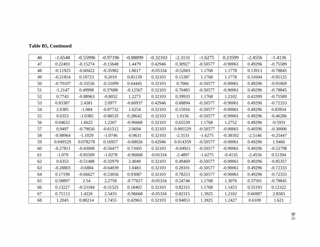
B-5
Table B5, Continued
46 -1.6548 -0.55996 -0.97196 -0.88899 -0.32103 -2.3131 -1.6275 0.23599 -2.4556 -1.4136 47 0.22493 -0.15274 -0.15648 1.4479 0.42946 0.30927 -0.50577 -0.90061 0.49296 -0.75589 48 -0.11925 -0.60422 -0.35982 1.8617 -0.05334 -0.52601 1.1768 1.1778 0.13913 -0.78845 49 -0.21854 0.10723 0.2019 0.85139 0.32103 0.15387 1.1768 1.1778 0.31604 -0.95125 50 -0.79107 -0.33536 -0.32099 0.64445 0.32103 0.7066 -0.50577 -0.90061 0.49296 -0.91869 51 -1.2147 0.49998 0.37688 -0.12567 0.32103 0.70483 -0.50577 -0.90061 0.49296 -0.78845 52 0.7743 -0.88963 -0.8052 1.2273 0.32103 0.39933 1.1768 1.2102 0.43399 -0.75589 53 0.83387 2.4381 2.0977 -0.60937 0.42946 0.68894 -0.50577 -0.90061 0.49296 -0.72333 54 2.0385 -1.084 -0.87732 1.6254 0.32103 0.15916 -0.50577 -0.90061 0.49296 0.83954 55 0.6353 -1.0385 -0.88535 0.28642 0.32103 1.0156 -0.50577 -0.90061 0.49296 -0.46286 56 0.04622 1.6625 1.2267 -0.96668 0.32103 0.65539 1.1768 1.2752 0.49296 -0.5931 57 0.9497 -0.79656 -0.61512 2.0694 0.32103 0.005529 -0.50577 -0.90061 0.49296 -0.30006 58 -0.98964 -1.1029 -1.0746 -0.9631 0.32103 -2.3131 -1.6275 -0.38102 -2.5146 -0.25447 59 0.049529 0.078278 0.16957 -0.68026 0.42946 0.014359 -0.50577 -0.90061 0.49296 1.9466 60 -0.27811 -0.43608 -0.56477 0.71605 0.32103 -0.04921 -0.50577 -0.90061 0.49296 -0.52798 61 -1.079 -0.85509 -1.0278 -0.96668 -0.05334 -2.4897 -1.6275 -0.4135 -2.4556 0.51394 62 0.6353 -0.51488 -0.32979 2.4049 0.32103 0.49469 -0.50577 -0.90061 0.49296 -0.85357 63 -0.28803 -0.6884 -0.64039 1.0483 0.32103 0.28101 -0.50577 -0.90061 0.49296 -0.72333 64 0.17198 -0.66627 -0.53056 0.93087 0.32103 0.78253 -0.50577 -0.90061 0.49296 -0.72333 65 0.58897 2.54 2.2758 -0.77657 -0.05334 0.24746 1.1768 1.3076 0.37501 -0.78845 66 0.13227 -0.53184 -0.31525 0.18402 0.32103 0.82315 1.1768 1.1453 0.55193 0.12322 67 0.75113 1.4226 2.5433 -0.96668 -0.05334 0.82315 1.3925 1.2102 0.66987 2.8583 68 1.2045 0.80214 1.7455 0.42963 0.32103 0.94853 1.3925 1.2427 0.6109 1.621
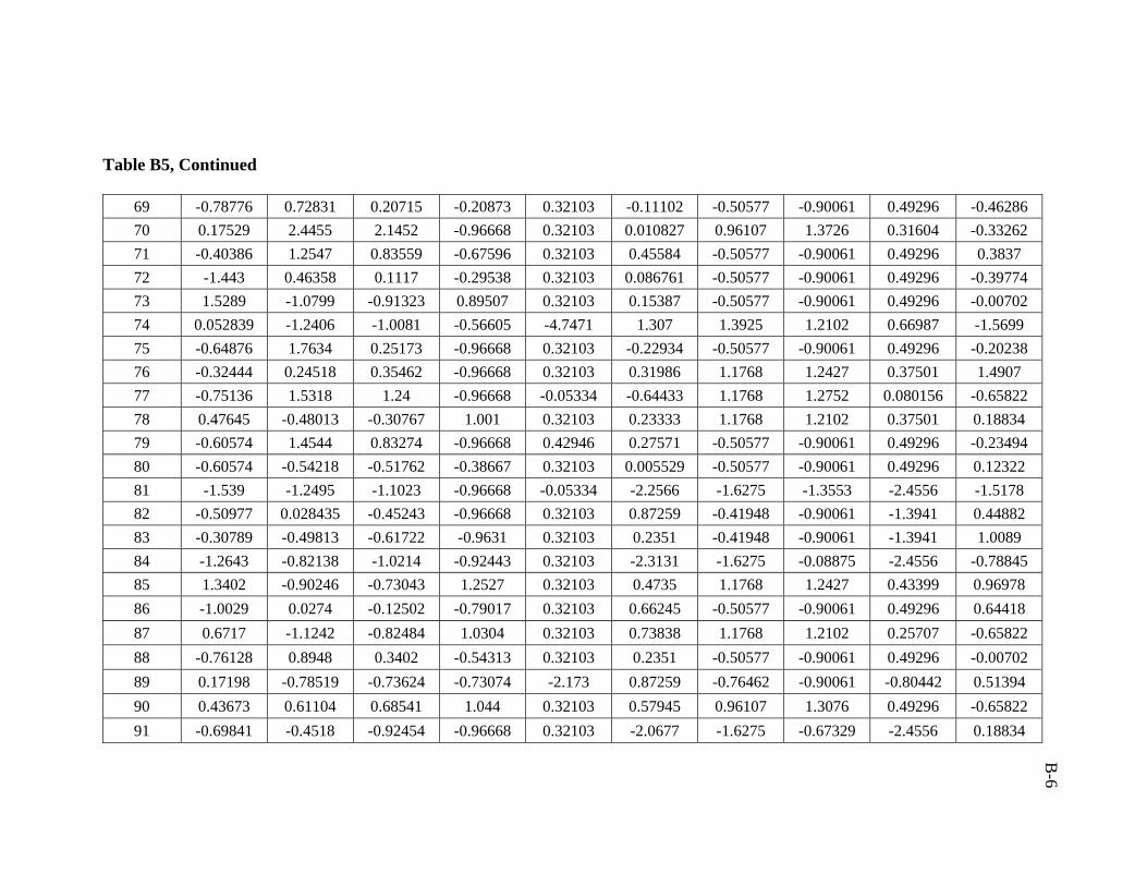
B-6
Table B5, Continued
69 -0.78776 0.72831 0.20715 -0.20873 0.32103 -0.11102 -0.50577 -0.90061 0.49296 -0.46286 70 0.17529 2.4455 2.1452 -0.96668 0.32103 0.010827 0.96107 1.3726 0.31604 -0.33262 71 -0.40386 1.2547 0.83559 -0.67596 0.32103 0.45584 -0.50577 -0.90061 0.49296 0.3837 72 -1.443 0.46358 0.1117 -0.29538 0.32103 0.086761 -0.50577 -0.90061 0.49296 -0.39774 73 1.5289 -1.0799 -0.91323 0.89507 0.32103 0.15387 -0.50577 -0.90061 0.49296 -0.00702 74 0.052839 -1.2406 -1.0081 -0.56605 -4.7471 1.307 1.3925 1.2102 0.66987 -1.5699 75 -0.64876 1.7634 0.25173 -0.96668 0.32103 -0.22934 -0.50577 -0.90061 0.49296 -0.20238 76 -0.32444 0.24518 0.35462 -0.96668 0.32103 0.31986 1.1768 1.2427 0.37501 1.4907 77 -0.75136 1.5318 1.24 -0.96668 -0.05334 -0.64433 1.1768 1.2752 0.080156 -0.65822 78 0.47645 -0.48013 -0.30767 1.001 0.32103 0.23333 1.1768 1.2102 0.37501 0.18834 79 -0.60574 1.4544 0.83274 -0.96668 0.42946 0.27571 -0.50577 -0.90061 0.49296 -0.23494 80 -0.60574 -0.54218 -0.51762 -0.38667 0.32103 0.005529 -0.50577 -0.90061 0.49296 0.12322 81 -1.539 -1.2495 -1.1023 -0.96668 -0.05334 -2.2566 -1.6275 -1.3553 -2.4556 -1.5178 82 -0.50977 0.028435 -0.45243 -0.96668 0.32103 0.87259 -0.41948 -0.90061 -1.3941 0.44882 83 -0.30789 -0.49813 -0.61722 -0.9631 0.32103 0.2351 -0.41948 -0.90061 -1.3941 1.0089 84 -1.2643 -0.82138 -1.0214 -0.92443 0.32103 -2.3131 -1.6275 -0.08875 -2.4556 -0.78845 85 1.3402 -0.90246 -0.73043 1.2527 0.32103 0.4735 1.1768 1.2427 0.43399 0.96978 86 -1.0029 0.0274 -0.12502 -0.79017 0.32103 0.66245 -0.50577 -0.90061 0.49296 0.64418 87 0.6717 -1.1242 -0.82484 1.0304 0.32103 0.73838 1.1768 1.2102 0.25707 -0.65822 88 -0.76128 0.8948 0.3402 -0.54313 0.32103 0.2351 -0.50577 -0.90061 0.49296 -0.00702 89 0.17198 -0.78519 -0.73624 -0.73074 -2.173 0.87259 -0.76462 -0.90061 -0.80442 0.51394 90 0.43673 0.61104 0.68541 1.044 0.32103 0.57945 0.96107 1.3076 0.49296 -0.65822 91 -0.69841 -0.4518 -0.92454 -0.96668 0.32103 -2.0677 -1.6275 -0.67329 -2.4556 0.18834
B-7
Table B5, Continued
92 0.23817 1.2565 2.3532 -0.36806 -0.05334 -0.34765 1.3925 1.2427 0.1981 1.621 93 0.8438 -0.68695 -0.33114 -0.96668 -4.7471 0.16623 1.3925 1.1453 0.1981 0.96978 94 -1.1518 0.2398 0.008314 0.12602 0.32103 -0.03332 -0.50577 -0.90061 0.49296 -0.72333 95 0.9166 -1.2363 -1.0556 0.44968 0.32103 0.1627 1.1768 1.0479 0.37501 -0.88613 96 -1.1981 0.35397 -0.79914 -0.96668 -0.05334 -2.2248 -1.6275 0.56074 -2.4556 -1.1792 97 0.83056 -1.0607 -0.80731 -0.96668 -4.7471 0.41875 1.3925 1.1778 0.43399 1.5559 98 -0.01666 -0.74093 -0.66697 0.24238 0.32103 0.30573 1.1768 1.1453 0.37501 -0.23494 99 1.1549 0.30371 0.67087 0.9971 0.32103 0.89025 -0.50577 -0.90061 0.49296 0.35114
100 0.65185 -0.1182 0.19845 1.2889 -0.05334 0.60241 1.1768 1.1128 0.49296 -0.65822 101 -0.4866 1.0483 0.5571 -0.53346 -0.05334 -0.08453 1.1768 1.2752 0.25707 -0.78845 102 0.60221 2.75 2.0579 -0.96668 -0.05334 0.24569 0.96107 1.0479 0.37501 -0.33262 103 -4.1766 -1.124 -0.94939 -0.87645 -0.05334 -0.28231 1.1768 1.0479 0.1981 -1.1141 104 -0.11925 -0.33536 -0.29446 1.0383 0.32103 0.31986 -0.50577 -0.90061 0.49296 -0.65822 105 1.2376 0.67805 1.5304 0.25062 -0.05334 1.1799 1.3925 1.2102 0.66987 1.9466 106 0.27126 0.098546 -0.0602 1.0394 0.32103 0.79313 -0.50577 -0.90061 0.49296 -0.56054 107 0.73127 -0.69688 -0.60821 -0.92013 -4.7471 0.47703 0.96107 1.3076 0.43399 -0.91869 108 -1.3471 -0.82138 -1.0888 -0.96668 0.32103 -2.276 -1.6275 0.30094 -2.4556 -0.62566 109 1.4362 -0.07394 -0.05184 2.2634 0.32103 0.95206 -0.50577 -0.90061 0.49296 -0.65822 110 0.64854 1.567 1.5364 -0.95128 -0.05334 0.39226 1.1768 1.2102 0.43399 1.7512 111 -2.1579 -1.1833 -1.0156 -0.68026 0.42946 -1.3118 -0.76462 -0.90061 -0.80442 -0.78845 112 -1.6482 -0.86812 -0.7636 -0.68885 0.32103 0.24393 -0.50577 -0.90061 0.49296 -0.75589 113 -0.01666 -0.32295 -0.31438 1.3032 0.32103 0.24746 1.1768 1.2427 0.37501 -0.91869 114 -1.3404 -0.28572 -0.9201 -0.96668 -0.05334 -3.0195 -1.6275 0.17104 -2.7505 0.44882
B-8
Table B5, Continued
115 2.0385 -1.084 -0.89401 1.6254 0.32103 0.14857 1.1768 1.0479 0.31604 0.83954 116 -0.02328 0.76078 0.61397 0.14321 -0.05334 -0.04215 1.1768 1.2102 0.25707 -0.78845 117 0.6353 -1.0385 -0.8074 0.33081 -0.05334 1.005 1.1768 1.0803 0.6109 -0.46286 118 0.50623 -0.32233 -0.17544 0.40672 0.32103 0.96442 -0.50577 -0.90061 0.49296 1.1651 119 -1.2544 1.021 -0.67302 -0.96668 0.32103 -2.3131 -1.6275 -0.47845 -2.4556 -1.2443 120 -1.7012 -1.1126 -1.0765 -0.96668 -0.05334 -2.4915 -1.6275 -0.60834 -2.4556 -0.56054 121 0.92653 -0.71942 -0.62848 -0.29538 0.42946 0.64832 -0.50577 -0.90061 0.49296 1.2954 122 0.72135 1.7328 2.9588 -0.68026 0.32103 0.74368 1.3925 1.2427 0.55193 1.4256 123 0.9166 -0.6762 -0.54137 -0.92801 -4.7471 0.51941 0.96107 1.3401 0.49296 -0.13726 124 -0.72819 1.5167 1.361 -0.96668 0.32103 -0.40946 1.1768 1.2102 0.13913 -0.65822 125 1.3667 -0.9796 -0.78338 -0.05442 0.42946 0.35695 -0.50577 -0.90061 0.49296 0.7093 126 -0.59581 0.98683 0.77873 -0.40171 0.32103 0.15563 -0.50577 -0.90061 0.49296 -0.13726 127 0.10579 -0.97918 -0.83796 -0.69923 0.32103 -0.71143 -0.50577 -0.90061 0.49296 1.1651 128 0.29112 -0.63214 -0.42116 -0.28285 0.42946 -0.17283 -0.50577 -0.90061 0.49296 0.83954 129 0.20176 -0.09069 -0.04538 1.233 0.32103 0.26865 -0.50577 -0.90061 0.49296 -0.5931 130 0.13888 -1.0476 -0.84928 -0.02363 -0.05334 -0.13221 0.96107 1.0479 0.25707 2.8583 131 -1.913 -0.91652 -1.0394 -0.96668 0.32103 -2.2248 -1.6275 -0.31607 -2.4556 -1.4722 132 0.92653 1.8983 2.9885 -0.96668 0.32103 0.91144 1.3925 1.3076 0.6109 1.4256 133 1.1119 1.7535 2.9865 -0.96668 -0.05334 0.83727 1.3925 1.2102 0.66987 3.1187 134 -0.19868 1.9303 1.3254 -0.86392 0.32103 -0.0916 1.1768 1.3076 0.25707 -0.2675 135 -0.71826 -0.48013 -0.4054 0.15896 0.32103 0.41346 -0.50577 -0.90061 0.49296 -0.65822 136 1.4792 -0.98332 -0.69673 1.6512 0.32103 0.71896 -0.50577 -0.90061 0.49296 -0.52798 137 0.75775 -0.35604 -0.34426 1.5037 0.32103 0.25982 -0.50577 -0.90061 0.49296 -0.36518
B-9
Table B5, Continued
138 0.15874 -0.50185 -0.03107 -0.21482 0.32103 0.83727 -0.50577 -0.90061 0.49296 0.77442 139 -1.8004 -0.74548 -1.085 -0.96668 0.32103 -2.276 -1.6275 0.56074 -2.4556 -1.3094 140 -1.2378 0.77505 0.49959 -0.32438 0.32103 0.13621 -0.50577 -0.90061 0.49296 -0.52798 141 2.1014 -1.1626 -0.97937 0.89507 0.32103 1.1269 -0.50577 -0.90061 0.49296 -0.20238 142 -0.66531 1.3159 0.91222 -0.80449 0.32103 -0.51012 1.1768 1.2752 0.13913 -0.13726 143 -1.2809 -0.72314 -1.0028 -0.96668 -0.05334 -2.465 -1.6275 0.00867 -2.4556 -0.20238 144 -1.0459 -1.1668 -1.0867 -0.96668 -0.05334 -2.2637 -1.6275 -0.25113 -2.4556 0.29253 145 -0.52962 0.34714 0.10869 -0.96668 0.32103 0.49822 -0.50577 -0.90061 0.49296 0.96978 146 -0.21854 0.2396 0.3664 -0.96632 -2.173 0.081464 0.96107 1.2427 0.31604 -0.91869 147 -0.1358 1.2437 0.89669 -0.58251 -0.05334 0.40816 1.1768 1.2427 0.43399 -0.65822 148 -0.62891 0.6582 1.3801 -0.56569 -0.05334 -0.34765 1.3925 1.2102 0.1981 0.83954 149 -0.02328 -0.749 -0.62154 1.3963 0.42946 -0.0916 -0.50577 -0.90061 0.49296 -0.72333 150 1.4263 -0.70763 -0.61415 2.363 0.32103 0.78253 -0.50577 -0.90061 0.49296 -0.72333 151 1.2806 -1.1833 -1.0582 -0.17902 0.32103 0.95559 -0.41948 -0.90061 -1.3941 -1.1792 152 0.1091 0.015405 0.27703 0.91511 -0.05334 0.74192 1.1768 1.2102 0.55193 -0.85357 153 -1.0988 0.73306 -0.66315 -0.96668 0.32103 -2.0677 -1.6275 0.20352 -2.4556 -0.8666 154 1.9822 -1.2104 -1.0037 0.92908 0.32103 0.67481 -0.50577 -0.90061 0.49296 -0.1047 155 1.4263 0.70287 1.1666 1.0257 0.32103 0.86023 -0.50577 -0.90061 0.49296 0.31858 156 1.1383 -0.76968 -0.67179 0.39383 0.32103 0.66422 -0.50577 -0.90061 0.49296 0.90466 157 -0.75136 -1.0514 -0.88569 -0.15252 0.32103 -0.97102 -0.50577 -0.90061 0.49296 -0.00702 158 1.0457 2.2588 1.8931 -0.71749 -0.05334 0.62537 0.96107 1.3726 0.49296 -0.00702 159 0.026363 -0.14922 0.043778 0.96667 -0.05334 0.24393 1.1768 1.1128 0.37501 -0.78845 160 -0.21854 0.10723 0.10642 0.85139 0.42946 0.15387 -0.50577 -0.90061 0.49296 -0.95125
B-10
Table B5, Continued
161 -0.39394 -0.85282 -0.7729 0.18975 0.32103 0.34458 -0.50577 -0.90061 0.49296 -0.72333 162 1.8499 -1.1459 -0.97869 -0.56175 0.32103 0.60064 -0.50577 -0.90061 0.49296 1.5559 163 1.3535 -0.92376 -0.59339 -0.96668 -3.5956 1.2064 1.3925 1.0479 0.37501 4.1606 164 0.15212 -0.27331 -0.3231 0.89507 0.32103 0.49292 -0.50577 -0.90061 0.49296 -0.07214 165 -0.63884 -0.23195 -0.26751 0.42963 0.32103 0.73662 -0.50577 -0.90061 0.49296 -0.78845 166 -0.98302 -0.81993 -1.0211 -0.96668 -0.05334 -2.1789 -1.6275 -0.08875 -2.4556 0.28602 167 1.4726 -0.92893 -0.77307 0.057281 0.32103 0.50881 -0.50577 -0.90061 0.49296 1.6535 168 -1.2478 -0.47868 -0.95659 -0.96668 -0.05334 -2.1789 -1.6275 0.17104 -2.4556 -0.16982 169 -0.46343 1.4985 0.94948 -0.60435 0.32103 0.19095 -0.50577 -0.90061 0.49296 -0.39774 170 0.96625 -0.80711 -0.70432 1.001 0.42946 0.98561 -0.50577 -0.90061 0.49296 -0.30006 171 -0.42703 -0.5732 -0.54425 0.66235 0.32103 0.86376 -0.50577 -0.90061 0.49296 -0.5931 172 -1.3206 0.93244 0.55817 -0.96668 0.42946 0.27218 -0.50577 -0.90061 0.49296 -0.20238 173 0.70149 -0.93513 -0.74728 1.3605 0.32103 -0.1587 -0.50577 -0.90061 0.49296 -0.2675 174 0.55918 0.31364 0.26597 -0.76905 0.32103 -0.13398 -0.50577 -0.90061 0.49296 2.2071 175 -0.89697 1.392 0.68697 -0.91691 0.42946 0.081464 -0.50577 -0.90061 0.49296 -0.52798 176 -0.5197 -0.75313 -0.64165 -0.13212 0.32103 0.27571 1.1768 1.0803 0.37501 -0.85357 177 0.21169 -0.19431 -0.16662 1.1897 0.32103 0.63949 -0.50577 -0.90061 0.49296 -0.5931 178 -1.3537 -0.47496 -0.95588 -0.96668 -0.05334 -2.4897 -1.6275 0.20352 -2.4556 -0.00702 179 0.64523 1.9742 1.4774 -0.72071 -0.05334 0.47526 1.1768 1.2752 0.43399 -0.52798 180 0.62868 0.22305 0.23106 1.8259 0.32103 0.000231 -0.50577 -0.90061 0.49296 -0.72333 181 0.006506 0.44848 0.32548 0.95271 -0.05334 -0.49246 1.1768 1.1778 0.13913 -0.82101 182 -1.9295 -0.39265 -0.45301 -0.14751 0.32103 0.17329 -0.50577 -0.90061 0.49296 -0.91869 183 -0.79107 -0.33536 -0.31235 0.64445 0.32103 0.15916 -0.50577 -0.90061 0.49296 -0.91869
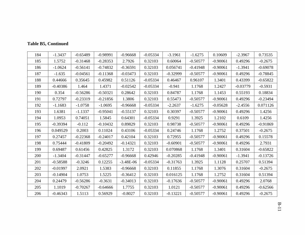
B-11
Table B5, Continued
184 -1.3437 -0.65489 -0.98991 -0.96668 -0.05334 -3.1961 -1.6275 0.10609 -2.3967 0.73535 185 1.5752 -0.31468 -0.28353 2.7926 0.32103 0.60064 -0.50577 -0.90061 0.49296 -0.2675 186 -1.0624 -0.56141 -0.74832 -0.36591 0.32103 0.056741 -0.41948 -0.90061 -1.3941 -0.69078 187 -1.635 -0.04561 -0.11368 -0.03473 0.32103 -0.32999 -0.50577 -0.90061 0.49296 -0.78845 188 0.44666 0.35645 0.45982 0.51126 -0.05334 0.46467 0.96107 1.3401 0.43399 -0.65822 189 -0.40386 1.464 1.4371 -0.02542 -0.05334 -0.941 1.1768 1.2427 -0.03779 -0.5931 190 0.354 -0.56286 -0.50321 0.28642 0.32103 0.84787 1.1768 1.1453 0.55193 0.18834 191 0.72797 -0.23319 -0.21856 1.3806 0.32103 0.55473 -0.50577 -0.90061 0.49296 -0.23494 192 -1.1683 -1.0758 -1.0695 -0.96668 -0.05334 -2.2637 -1.6275 -0.05628 -2.4556 0.071126 193 1.6381 -1.1337 -0.95041 -0.55137 0.32103 0.30397 -0.50577 -0.90061 0.49296 1.4256 194 1.0953 0.74051 1.5845 0.64301 -0.05334 0.9291 1.3925 1.2102 0.6109 1.4256 195 -0.39394 -0.112 -0.10432 0.89829 0.32103 0.98738 -0.50577 -0.90061 0.49296 -0.91869 196 0.049529 0.2003 0.11024 0.43106 -0.05334 0.24746 1.1768 1.2752 0.37501 -0.2675 197 0.27457 -0.22368 -0.24017 0.42104 0.32103 0.72955 -0.50577 -0.90061 0.49296 0.15578 198 0.75444 -0.41809 -0.20492 -0.14321 0.32103 -0.60901 -0.50577 -0.90061 0.49296 2.7931 199 0.69487 0.61456 0.42825 1.3172 0.32103 0.070868 1.1768 1.3401 0.31604 -0.65822 200 -1.3404 -0.31447 -0.65277 -0.96668 0.42946 -0.20285 -0.41948 -0.90061 -1.3941 -0.13726 201 -0.58588 -0.3246 0.12255 -3.48E-06 -0.05334 -0.31763 1.3925 1.1128 0.25707 0.51394 202 -0.01997 2.0921 1.5383 -0.96668 0.32103 0.11855 1.1768 1.3076 0.31604 -0.2675 203 -0.14904 1.0753 1.5225 -0.36412 0.32103 0.016125 1.1768 1.2752 0.31604 0.51394 204 0.24479 -0.56286 -0.3631 -0.34013 0.32103 -0.17636 -0.50577 -0.90061 0.49296 2.0768 205 1.1019 -0.70267 -0.64666 1.7755 0.32103 1.0121 -0.50577 -0.90061 0.49296 -0.62566 206 -0.46343 1.5113 0.56929 -0.8027 0.32103 -0.13221 -0.50577 -0.90061 0.49296 -0.2675
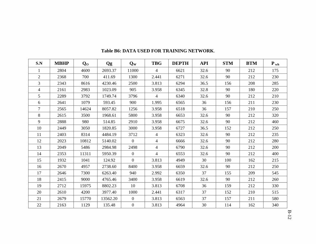
B-12
Table B6: DATA USED FOR TRAINING NETWORK.
S.N MBHP QO Qg QW TBG DEPTH API STM BTM P wh
1 2804 4600 2693.37 11000 4 6621 32.6 90 212 175 2 2368 700 411.69 1300 2.441 6271 32.6 90 212 230 3 2343 8616 4230.46 2500 3.813 6294 36.5 156 208 285 4 2161 2983 1023.09 905 3.958 6345 32.8 90 180 220 5 2289 3792 1749.74 3796 4 6340 32.6 90 212 210 6 2641 1079 593.45 900 1.995 6565 36 156 211 230 7 2565 14624 8057.82 1256 3.958 6518 36 157 210 250 8 2615 3500 1968.61 5800 3.958 6653 32.6 90 212 320 9 2888 980 514.85 2910 3.958 6675 32.6 90 212 460
10 2449 3050 1820.85 3000 3.958 6727 36.5 152 212 250 11 2403 8314 4484.19 3712 4 6323 32.6 90 212 235 12 2023 10812 5140.02 0 4 6666 32.6 90 212 280 13 2049 5486 2984.98 2498 4 6790 32.6 90 212 200 14 2353 11311 5950.39 0 4 6553 32.6 90 212 400 15 1932 1041 124.92 0 3.813 4949 30 100 162 215 16 2670 4957 2738.60 8400 3.958 6659 32.6 90 212 250 17 2646 7300 6263.40 940 2.992 6350 37 155 209 545 18 2415 9000 4765.46 3400 3.958 6619 32.6 90 212 260 19 2712 15975 8802.23 10 3.813 6708 36 159 212 330 20 2610 4200 3977.40 1000 2.441 6317 37 152 210 515 21 2679 15770 13562.20 0 3.813 6563 37 157 211 580 22 2163 1129 135.48 0 3.813 4964 30 114 162 340
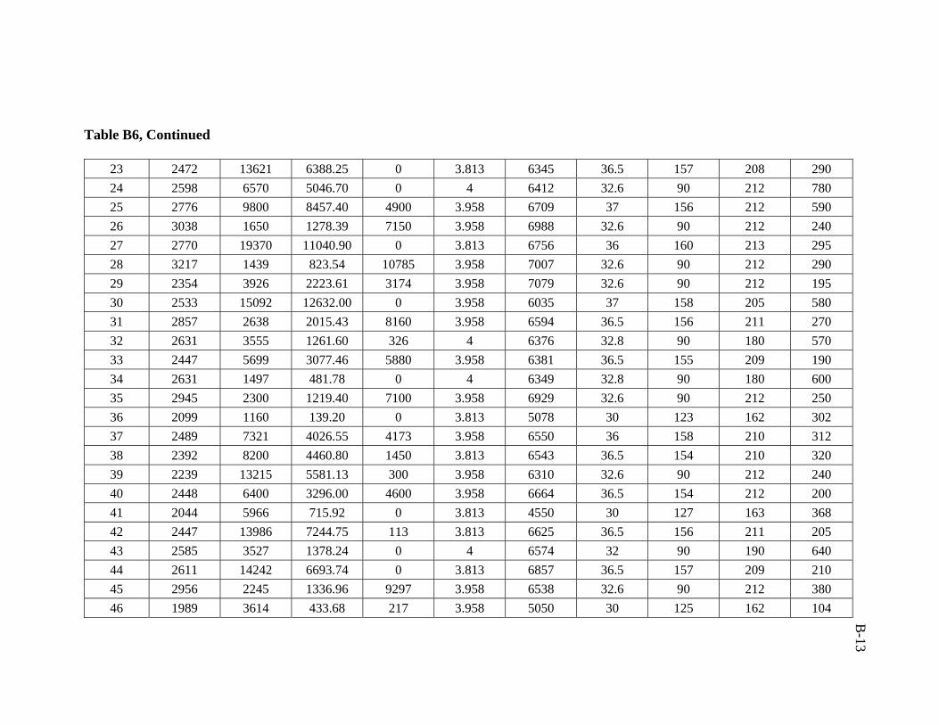
B-13
Table B6, Continued
23 2472 13621 6388.25 0 3.813 6345 36.5 157 208 290 24 2598 6570 5046.70 0 4 6412 32.6 90 212 780 25 2776 9800 8457.40 4900 3.958 6709 37 156 212 590 26 3038 1650 1278.39 7150 3.958 6988 32.6 90 212 240 27 2770 19370 11040.90 0 3.813 6756 36 160 213 295 28 3217 1439 823.54 10785 3.958 7007 32.6 90 212 290 29 2354 3926 2223.61 3174 3.958 7079 32.6 90 212 195 30 2533 15092 12632.00 0 3.958 6035 37 158 205 580 31 2857 2638 2015.43 8160 3.958 6594 36.5 156 211 270 32 2631 3555 1261.60 326 4 6376 32.8 90 180 570 33 2447 5699 3077.46 5880 3.958 6381 36.5 155 209 190 34 2631 1497 481.78 0 4 6349 32.8 90 180 600 35 2945 2300 1219.40 7100 3.958 6929 32.6 90 212 250 36 2099 1160 139.20 0 3.813 5078 30 123 162 302 37 2489 7321 4026.55 4173 3.958 6550 36 158 210 312 38 2392 8200 4460.80 1450 3.813 6543 36.5 154 210 320 39 2239 13215 5581.13 300 3.958 6310 32.6 90 212 240 40 2448 6400 3296.00 4600 3.958 6664 36.5 154 212 200 41 2044 5966 715.92 0 3.813 4550 30 127 163 368 42 2447 13986 7244.75 113 3.813 6625 36.5 156 211 205 43 2585 3527 1378.24 0 4 6574 32 90 190 640 44 2611 14242 6693.74 0 3.813 6857 36.5 157 209 210 45 2956 2245 1336.96 9297 3.958 6538 32.6 90 212 380 46 1989 3614 433.68 217 3.958 5050 30 125 162 104
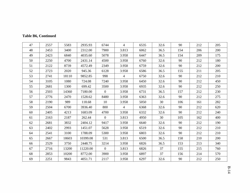
B-14
Table B6, Continued
47 2557 5583 2935.93 6744 4 6535 32.6 90 212 205 48 2453 3400 2312.00 7900 3.813 6062 36.5 154 206 200 49 2423 6840 4035.60 5078 3.958 6447 36.5 154 209 175 50 2250 4700 2431.14 4500 3.958 6760 32.6 90 212 180 51 2122 8739 4572.49 2349 3.958 6759 32.6 90 212 200 52 2723 2020 945.36 6128 3.958 6586 36.5 155 211 205 53 2741 18110 9852.85 998 4 6750 32.6 90 212 210 54 3105 1080 724.08 7240 3.958 6450 32.6 90 212 450 55 2681 1300 699.42 3500 3.958 6935 32.6 90 212 250 56 2503 14360 7180.00 0 3.958 6731 36.5 157 212 230 57 2776 2470 1528.62 8480 3.958 6363 32.6 90 212 275 58 2190 989 118.68 10 3.958 5050 30 106 161 282 59 2504 6700 3936.40 800 4 6368 32.6 90 212 620 60 2405 4213 1683.09 4700 3.958 6332 32.6 90 212 240 61 2163 2187 262.44 0 3.813 4950 30 105 162 400 62 2681 3832 2404.12 9417 3.958 6640 32.6 90 212 190 63 2402 2993 1451.07 5628 3.958 6519 32.6 90 212 210 64 2541 3100 1788.09 5300 3.958 6803 32.6 90 212 210 65 2667 18603 10399.08 531 3.813 6500 36.5 158 210 200 66 2529 3750 2448.75 3214 3.958 6826 36.5 153 213 340 67 2716 13200 11220.00 0 3.813 6826 37 155 215 760 68 2853 10200 8772.00 3900 3.958 6897 37 156 214 570 69 2251 9843 4051.71 2117 3.958 6297 32.6 90 212 250
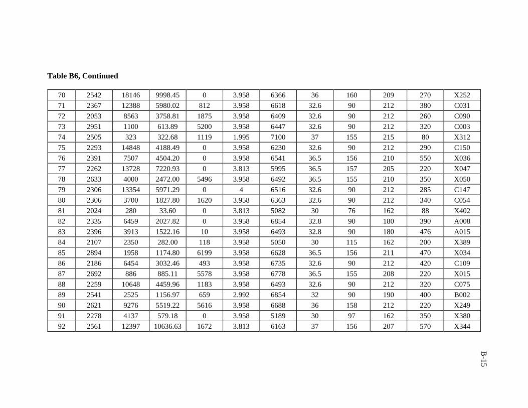
B-15
Table B6, Continued
70 2542 18146 9998.45 0 3.958 6366 36 160 209 270 X252 71 2367 12388 5980.02 812 3.958 6618 32.6 90 212 380 C031 72 2053 8563 3758.81 1875 3.958 6409 32.6 90 212 260 C090 73 2951 1100 613.89 5200 3.958 6447 32.6 90 212 320 C003 74 2505 323 322.68 1119 1.995 7100 37 155 215 80 X312 75 2293 14848 4188.49 0 3.958 6230 32.6 90 212 290 C150 76 2391 7507 4504.20 0 3.958 6541 36.5 156 210 550 X036 77 2262 13728 7220.93 0 3.813 5995 36.5 157 205 220 X047 78 2633 4000 2472.00 5496 3.958 6492 36.5 155 210 350 X050 79 2306 13354 5971.29 0 4 6516 32.6 90 212 285 C147 80 2306 3700 1827.80 1620 3.958 6363 32.6 90 212 340 C054 81 2024 280 33.60 0 3.813 5082 30 76 162 88 X402 82 2335 6459 2027.82 0 3.958 6854 32.8 90 180 390 A008 83 2396 3913 1522.16 10 3.958 6493 32.8 90 180 476 A015 84 2107 2350 282.00 118 3.958 5050 30 115 162 200 X389 85 2894 1958 1174.80 6199 3.958 6628 36.5 156 211 470 X034 86 2186 6454 3032.46 493 3.958 6735 32.6 90 212 420 C109 87 2692 886 885.11 5578 3.958 6778 36.5 155 208 220 X015 88 2259 10648 4459.96 1183 3.958 6493 32.6 90 212 320 C075 89 2541 2525 1156.97 659 2.992 6854 32 90 190 400 B002 90 2621 9276 5519.22 5616 3.958 6688 36 158 212 220 X249 91 2278 4137 579.18 0 3.958 5189 30 97 162 350 X380 92 2561 12397 10636.63 1672 3.813 6163 37 156 207 570 X344
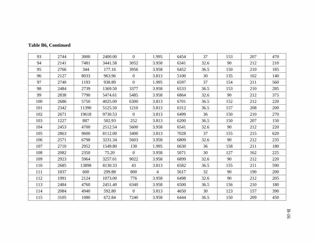
B-16
Table B6, Continued
93 2744 3000 2400.00 0 1.995 6454 37 153 207 470 94 2141 7481 3441.58 3052 3.958 6341 32.6 90 212 210 95 2766 344 177.16 3956 3.958 6452 36.5 150 210 185 96 2127 8033 963.96 0 3.813 5100 30 135 162 140 97 2740 1193 938.89 0 1.995 6597 37 154 211 560 98 2484 2739 1369.50 3377 3.958 6533 36.5 153 210 285 99 2838 7790 5474.61 5485 3.958 6864 32.6 90 212 375
100 2686 5750 4025.00 6300 3.813 6701 36.5 152 212 220 101 2342 11390 5125.50 1210 3.813 6312 36.5 157 208 200 102 2671 19618 9730.53 0 3.813 6499 36 150 210 270 103 1227 887 502.93 252 3.813 6200 36.5 150 207 150 104 2453 4700 2512.54 5600 3.958 6541 32.6 90 212 220 105 2863 9600 8112.00 3400 3.813 7028 37 155 215 620 106 2571 6798 3231.34 5603 3.958 6809 32.6 90 212 235 107 2710 2952 1549.80 130 1.995 6630 36 158 211 180 108 2082 2350 75.20 0 3.958 5071 30 127 162 225 109 2923 5964 3257.01 9022 3.958 6899 32.6 90 212 220 110 2685 13898 8130.33 43 3.813 6582 36.5 155 211 590 111 1837 600 299.88 800 4 5617 32 90 190 200 112 1991 2124 1073.00 776 3.958 6498 32.6 90 212 205 113 2484 4760 2451.40 6340 3.958 6500 36.5 156 210 180 114 2084 4940 592.80 0 3.813 4650 30 123 157 390 115 3105 1080 672.84 7240 3.958 6444 36.5 150 209 450
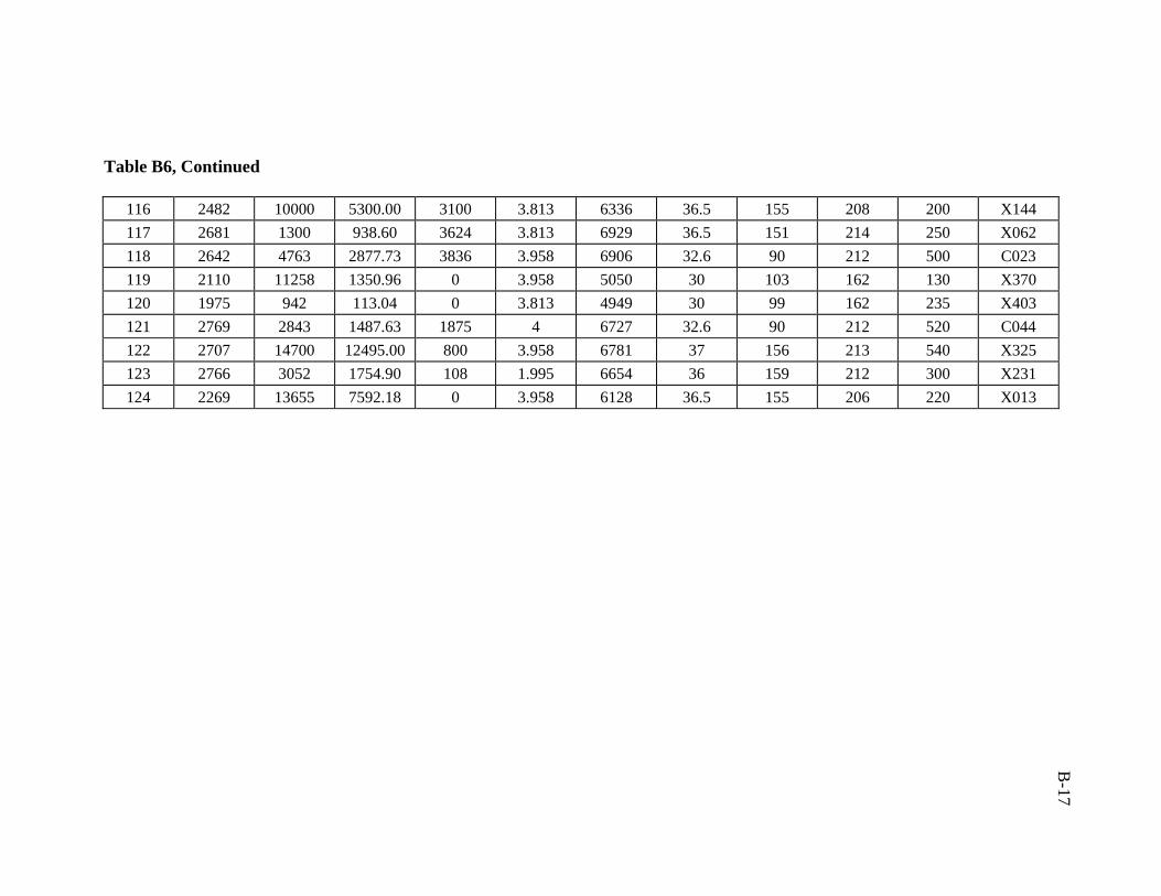
B-17
Table B6, Continued
116 2482 10000 5300.00 3100 3.813 6336 36.5 155 208 200 X144 117 2681 1300 938.60 3624 3.813 6929 36.5 151 214 250 X062 118 2642 4763 2877.73 3836 3.958 6906 32.6 90 212 500 C023 119 2110 11258 1350.96 0 3.958 5050 30 103 162 130 X370 120 1975 942 113.04 0 3.813 4949 30 99 162 235 X403 121 2769 2843 1487.63 1875 4 6727 32.6 90 212 520 C044 122 2707 14700 12495.00 800 3.958 6781 37 156 213 540 X325 123 2766 3052 1754.90 108 1.995 6654 36 159 212 300 X231 124 2269 13655 7592.18 0 3.958 6128 36.5 155 206 220 X013
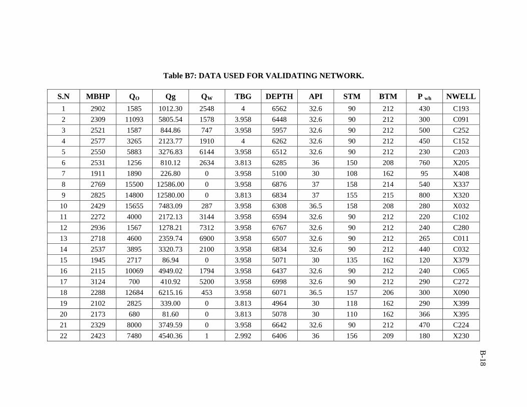
B-18
Table B7: DATA USED FOR VALIDATING NETWORK.
S.N MBHP QO Qg QW TBG DEPTH API STM BTM P wh NWELL1 2902 1585 1012.30 2548 4 6562 32.6 90 212 430 C193 2 2309 11093 5805.54 1578 3.958 6448 32.6 90 212 300 C091 3 2521 1587 844.86 747 3.958 5957 32.6 90 212 500 C252 4 2577 3265 2123.77 1910 4 6262 32.6 90 212 450 C152 5 2550 5883 3276.83 6144 3.958 6512 32.6 90 212 230 C203 6 2531 1256 810.12 2634 3.813 6285 36 150 208 760 X205 7 1911 1890 226.80 0 3.958 5100 30 108 162 95 X408 8 2769 15500 12586.00 0 3.958 6876 37 158 214 540 X337 9 2825 14800 12580.00 0 3.813 6834 37 155 215 800 X320
10 2429 15655 7483.09 287 3.958 6308 36.5 158 208 280 X032 11 2272 4000 2172.13 3144 3.958 6594 32.6 90 212 220 C102 12 2936 1567 1278.21 7312 3.958 6767 32.6 90 212 240 C280 13 2718 4600 2359.74 6900 3.958 6507 32.6 90 212 265 C011 14 2537 3895 3320.73 2100 3.958 6834 32.6 90 212 440 C032 15 1945 2717 86.94 0 3.958 5071 30 135 162 120 X379 16 2115 10069 4949.02 1794 3.958 6437 32.6 90 212 240 C065 17 3124 700 410.92 5200 3.958 6998 32.6 90 212 290 C272 18 2288 12684 6215.16 453 3.958 6071 36.5 157 206 300 X090 19 2102 2825 339.00 0 3.813 4964 30 118 162 290 X399 20 2173 680 81.60 0 3.813 5078 30 110 162 366 X395 21 2329 8000 3749.59 0 3.958 6642 32.6 90 212 470 C224 22 2423 7480 4540.36 1 2.992 6406 36 156 209 180 X230
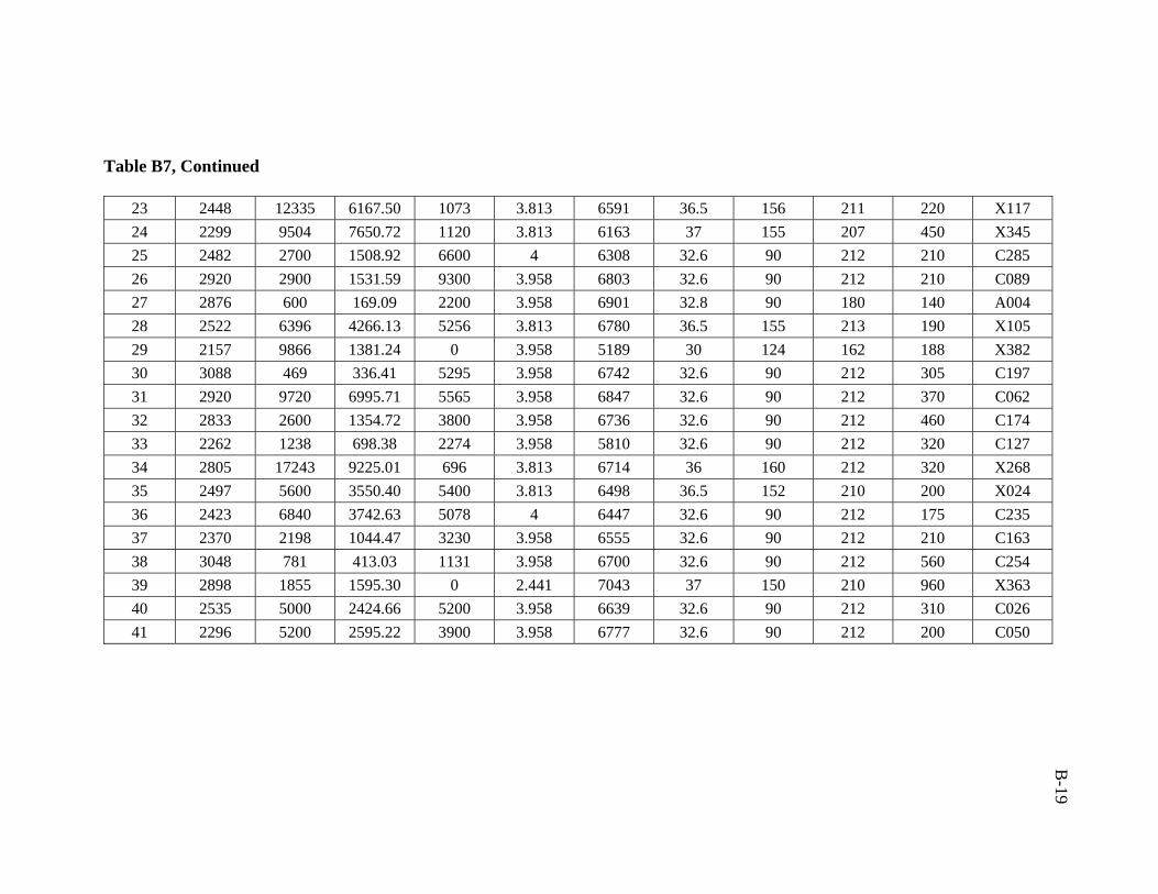
B-19
Table B7, Continued
23 2448 12335 6167.50 1073 3.813 6591 36.5 156 211 220 X117 24 2299 9504 7650.72 1120 3.813 6163 37 155 207 450 X345 25 2482 2700 1508.92 6600 4 6308 32.6 90 212 210 C285 26 2920 2900 1531.59 9300 3.958 6803 32.6 90 212 210 C089 27 2876 600 169.09 2200 3.958 6901 32.8 90 180 140 A004 28 2522 6396 4266.13 5256 3.813 6780 36.5 155 213 190 X105 29 2157 9866 1381.24 0 3.958 5189 30 124 162 188 X382 30 3088 469 336.41 5295 3.958 6742 32.6 90 212 305 C197 31 2920 9720 6995.71 5565 3.958 6847 32.6 90 212 370 C062 32 2833 2600 1354.72 3800 3.958 6736 32.6 90 212 460 C174 33 2262 1238 698.38 2274 3.958 5810 32.6 90 212 320 C127 34 2805 17243 9225.01 696 3.813 6714 36 160 212 320 X268 35 2497 5600 3550.40 5400 3.813 6498 36.5 152 210 200 X024 36 2423 6840 3742.63 5078 4 6447 32.6 90 212 175 C235 37 2370 2198 1044.47 3230 3.958 6555 32.6 90 212 210 C163 38 3048 781 413.03 1131 3.958 6700 32.6 90 212 560 C254 39 2898 1855 1595.30 0 2.441 7043 37 150 210 960 X363 40 2535 5000 2424.66 5200 3.958 6639 32.6 90 212 310 C026 41 2296 5200 2595.22 3900 3.958 6777 32.6 90 212 200 C050
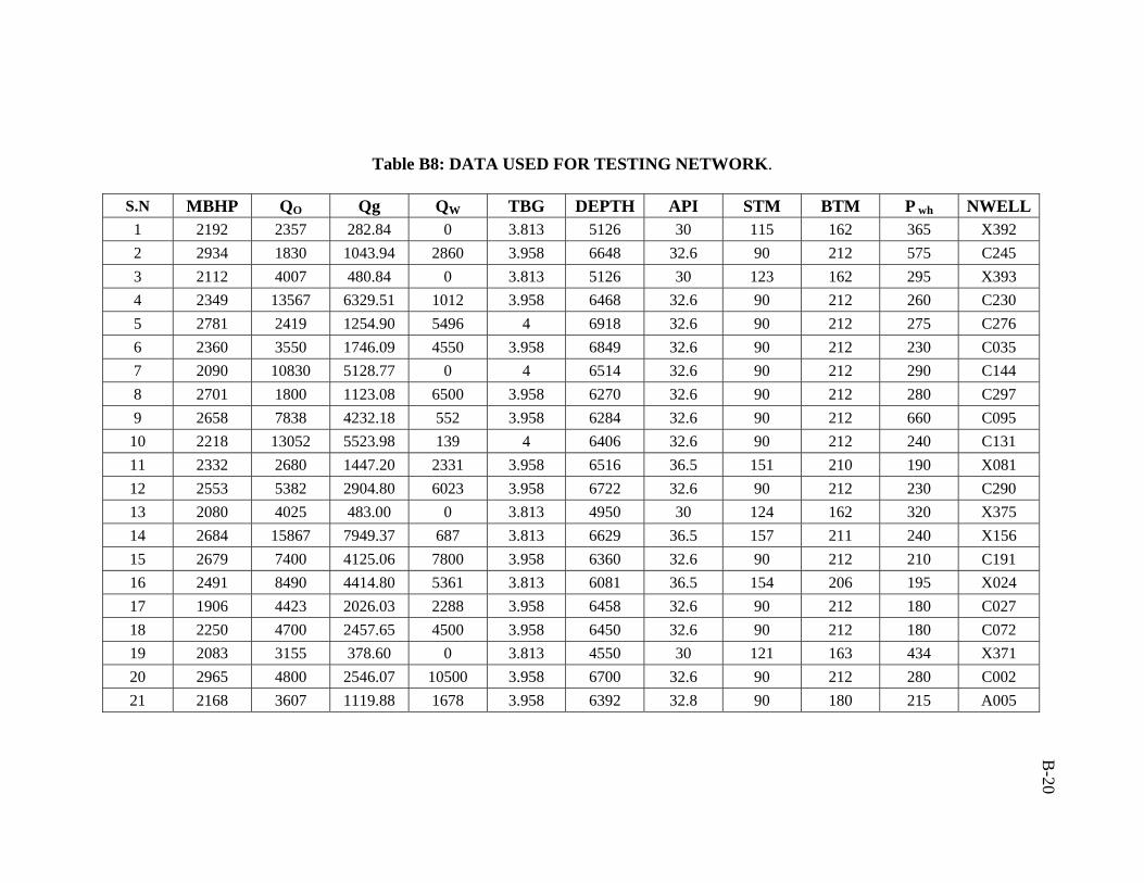
B-20
Table B8: DATA USED FOR TESTING NETWORK.
S.N MBHP QO Qg QW TBG DEPTH API STM BTM P wh NWELL1 2192 2357 282.84 0 3.813 5126 30 115 162 365 X392 2 2934 1830 1043.94 2860 3.958 6648 32.6 90 212 575 C245 3 2112 4007 480.84 0 3.813 5126 30 123 162 295 X393 4 2349 13567 6329.51 1012 3.958 6468 32.6 90 212 260 C230 5 2781 2419 1254.90 5496 4 6918 32.6 90 212 275 C276 6 2360 3550 1746.09 4550 3.958 6849 32.6 90 212 230 C035 7 2090 10830 5128.77 0 4 6514 32.6 90 212 290 C144 8 2701 1800 1123.08 6500 3.958 6270 32.6 90 212 280 C297 9 2658 7838 4232.18 552 3.958 6284 32.6 90 212 660 C095
10 2218 13052 5523.98 139 4 6406 32.6 90 212 240 C131 11 2332 2680 1447.20 2331 3.958 6516 36.5 151 210 190 X081 12 2553 5382 2904.80 6023 3.958 6722 32.6 90 212 230 C290 13 2080 4025 483.00 0 3.813 4950 30 124 162 320 X375 14 2684 15867 7949.37 687 3.813 6629 36.5 157 211 240 X156 15 2679 7400 4125.06 7800 3.958 6360 32.6 90 212 210 C191 16 2491 8490 4414.80 5361 3.813 6081 36.5 154 206 195 X024 17 1906 4423 2026.03 2288 3.958 6458 32.6 90 212 180 C027 18 2250 4700 2457.65 4500 3.958 6450 32.6 90 212 180 C072 19 2083 3155 378.60 0 3.813 4550 30 121 163 434 X371 20 2965 4800 2546.07 10500 3.958 6700 32.6 90 212 280 C002 21 2168 3607 1119.88 1678 3.958 6392 32.8 90 180 215 A005
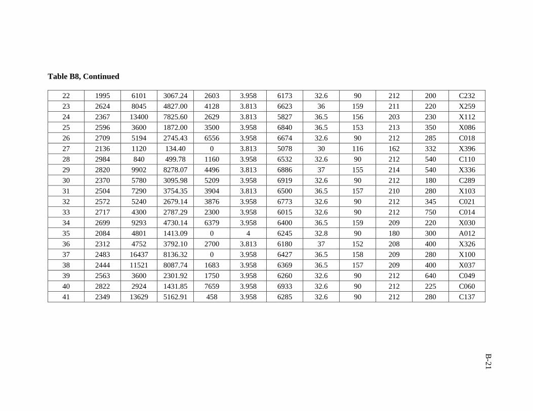
B-21
Table B8, Continued
22 1995 6101 3067.24 2603 3.958 6173 32.6 90 212 200 C232 23 2624 8045 4827.00 4128 3.813 6623 36 159 211 220 X259 24 2367 13400 7825.60 2629 3.813 5827 36.5 156 203 230 X112 25 2596 3600 1872.00 3500 3.958 6840 36.5 153 213 350 X086 26 2709 5194 2745.43 6556 3.958 6674 32.6 90 212 285 C018 27 2136 1120 134.40 0 3.813 5078 30 116 162 332 X396 28 2984 840 499.78 1160 3.958 6532 32.6 90 212 540 C110 29 2820 9902 8278.07 4496 3.813 6886 37 155 214 540 X336 30 2370 5780 3095.98 5209 3.958 6919 32.6 90 212 180 C289 31 2504 7290 3754.35 3904 3.813 6500 36.5 157 210 280 X103 32 2572 5240 2679.14 3876 3.958 6773 32.6 90 212 345 C021 33 2717 4300 2787.29 2300 3.958 6015 32.6 90 212 750 C014 34 2699 9293 4730.14 6379 3.958 6400 36.5 159 209 220 X030 35 2084 4801 1413.09 0 4 6245 32.8 90 180 300 A012 36 2312 4752 3792.10 2700 3.813 6180 37 152 208 400 X326 37 2483 16437 8136.32 0 3.958 6427 36.5 158 209 280 X100 38 2444 11521 8087.74 1683 3.958 6369 36.5 157 209 400 X037 39 2563 3600 2301.92 1750 3.958 6260 32.6 90 212 640 C049 40 2822 2924 1431.85 7659 3.958 6933 32.6 90 212 225 C060 41 2349 13629 5162.91 458 3.958 6285 32.6 90 212 280 C137
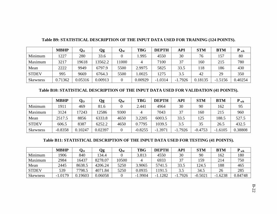
B-22
Table B9: STATISTICAL DESCRIPTION OF THE INPUT DATA USED FOR TRAINING (124 POINTS).
MBHP QO Qg QW TBG DEPTH API STM BTM P wh Minimum 1227 280 33.6 0 1.995 4550 30 76 157 80 Maximum 3217 19618 13562.2 11000 4 7100 37 160 215 780 Mean 2222 9949 6797.9 5500 2.9975 5825 33.5 118 186 430 STDEV 995 9669 6764.3 5500 1.0025 1275 3.5 42 29 350 Skewness 0.71362 0.05316 0.00913 0 0.00929 -1.0314 -1.7926 0.18135 -1.5156 0.40254
Table B10: STATISTICAL DESCRIPTION OF THE INPUT DATA USED FOR VALIDATION (41 POINTS).
MBHP QO Qg QW TBG DEPTH API STM BTM P wh
Minimum 1911 469 81.6 0 2.441 4964 30 90 162 95 Maximum 3124 17243 12586 9300 4 7043 37 160 215 960 Mean 2517.5 8856 6333.8 4650 3.2205 6003.5 33.5 125 188.5 527.5 STDEV 606.5 8387 6252.2 4650 0.7795 1039.5 3.5 35 26.5 432.5 Skewness -0.8358 0.10247 0.02397 0 -0.8255 -1.3971 -1.7926 -0.4753 -1.6105 0.38808
Table B11: STATISTICAL DESCRIPTION OF THE INPUT DATA USED FOR TESTING (41 POINTS).
MBHP QO Qg QW TBG DEPTH API STM BTM P wh
Minimum 1906 840 134.4 0 3.813 4550 30 90 162 180 Maximum 2984 16437 8278.07 10500 4 6933 37 159 214 750 Mean 2445 8638.5 4206.24 5250 3.9065 5741.5 33.5 124.5 188 465 STDEV 539 7798.5 4071.84 5250 0.0935 1191.5 3.5 34.5 26 285 Skewness -1.0179 0.19603 0.06058 0 -1.9904 -1.1282 -1.7926 -0.5021 -1.6238 0.84748

APPENDIX C
PROGRAM LISTING

C-1
APPENDIX C
PROGRAM LISTING
MAIN MODEL PROGRAM
close all; %close all figure windows clear all; %Clears all variables and other classes of data too. % To reduce the risk of confusing errors. % Step(1) Processing of the data: % =============================== % Step (2) Reading the input file % =============================== % Loads data and prepares it for a neural network. ndata= xlsread('main_file.xls'); % % Step (3) Normalizing the trainning data % ======================================= % Putting the data in the range of zero and one. % ********************************************** for i=1:10 meana(1,i)=mean(ndata(1:165,i)); stda(1,i)=std(ndata(1:165,i)); anormal(:,i)=(ndata(:,i)-meana(1,i))/stda(1,i); end % %60% of data will be used for trainning %20% of data will be used for cross-validation %20% of data will be used for testing for i=1:124 atr(i,:)=anormal(i,:); end for i=125:165 aval(i-124,:)=anormal(i,:); end % for i=166:length(anormal) atest(i-165,:)=anormal(i,:); end % Step (4) Generating Network structure % ==================================== % Back propagation: Batch gradient descent method with momentum % **************************************************************** % T=atr(:,1)';
C-2
P=atr(:,2:10)'; TV.P=atest(:,2:10)'; TV.T=atest(:,1)'; VV.T=aval(:,1)'; VV.P=aval(:,2:10)'; % S1=6; % Number of neurons in the first hidden layer S2=3; % Number of neurons in the second hidden layer S3=3; % Number of neurons in the third hidden layer S4=1; % Number of output variables (in our case PBHP) net=newff(minmax(P),[S1 S2 S3 S4],{'tansig' 'tansig' 'tansig' 'purelin'},'trainbfg'); net=init(net); net.trainParam.epochs = 350; %Max number of iterations net.trainParam.goal = 0.0; %Error tolerance; stopping criterion net.trainParam.max_fail =15 ; %Maximum validation failures net.trainParam.mem_reduc = 3 %Factor to use for memory/speed tradeoff net.trainParam.min_grad = 1e-15 %Minimum performance gradient net.trainParam.mu = 0.5 %Initial Mu net.trainParam.mu_dec = 0.9 %Mu decrease factor net.trainParam.mu_inc = 10 %Mu increase factor net.trainParam.mu_max = 1e10 %Maximum Mu net.trainParam.show = 5; %The result is shown at every 5th iteration
(epoch) net.trainParam.time = inf %Maximum time to train in seconds net.trainParam.lr_inc = 0.25 net.trainParam.lr = 0.750; %Learning rate used in some gradient schemes [net,tr]=train(net,P,T,[],[],VV,TV); % Plotting the network error progress for training, testing, and validation % data figure plot(tr.epoch,tr.perf,tr.epoch,tr.vperf,tr.epoch,tr.tperf) legend('Training','Validation','Test',-1); title('Training, Validation, Test Progress') ylabel('Squared Error'); xlabel('Epoch') set(gcf, 'color', 'white') grid off % % Detect whether the net simulates the input data % for testing data only % ********************* figure y1=sim(net,TV.P); plot(TV.T,'-r*'); refline(0,0) hold
C-3
plot(y1,':ko'); grid off set(gcf, 'color', 'white') title('Graph of Simulated network for Testing set') xlabel('Data Point No') ylabel('output of network and errors') legend('Actual BHP','ref. line','Predicted BHP') % Detect whether the net simulates the input data % for training data only % ********************** figure y2=sim(net,P); plot(T,'-r*'); refline(0,0) hold plot(y2,':ko'); grid off set(gcf, 'color', 'white') title('Graph of Simulated network for Training set') xlabel('Data Point No') ylabel('output of network and errors') legend('Actual BHP','ref. line','Predicted BHP') % Detect whether the net simulates the input data % for validation data only % ********************** figure y3=sim(net,VV.P); plot(VV.T,'-r*'); refline(0,0) hold plot(y3,':ko'); grid off set(gcf, 'color', 'white') title('Graph of Simulated network for Validation set') xlabel('Data Point No') ylabel('output of network and errors') legend('Actual BHP','ref. line','Predicted BHP') colormap gray % Evaluation of actual and estimated targets % ------------------------------------------ % firstly, for testing set: % ========================= Pred_tt=(y1*stda(1,1))+meana(1,1); Calc_tt=ndata(166:length(ndata),1);
C-4
% secondly, for validation set: % ============================ Pred_v=(y3*stda(1,1))+meana(1,1); Calc_v=ndata(125:165,1); % thirdly, for training set: % ============================ Pred_t=(y2*stda(1,1))+meana(1,1); Calc_t=ndata(1:124,1); % Evaluating Relative Error for training set: %=========================================== Et=(Calc_t'-Pred_t)./Calc_t'*100; [q,z] = size(Et); figure % plot(Calc_t',Pred_t,'o') grid off set(gcf, 'color', 'white') %axis ([1500,3500,1500,3500]) title('Graph of Predicted HP vs. Calculated HP'); xlabel('Calculated BHP "psig"'); ylabel('Predicted BHP "psig"') legend('Training set') % Addding Reference Line with 45 degree slope refline(1,0) % Evaluating the correlation coefficient for training set: % ======================================================== Rt=corrcoef(Pred_t,Calc_t); Rt2=min(Rt(:,2)); gtext(['correlation coefficient = (' num2str(Rt2) ')']); % Evaluating Relative Error for validation set: %=========================================== Ev=(Calc_v'-Pred_v)./Calc_v'*100; [m,n] = size(Ev); figure % plot(Calc_v',Pred_v,'o') grid off set(gcf, 'color', 'white') %axis ([1500,3500,1500,3500]) title('Graph of Predicted BHP vs. Calculated BHP'); xlabel('Calculated BHP "psig"');
C-5
ylabel('Predicted BHP "psig"') legend('Validation set') % Addding Reference Line with 45 degree slope refline(1,0) % Evaluating the correlation coefficient for validation set: % ======================================================== Rv=corrcoef(Pred_v,Calc_v); Rv2=min(Rv(:,2)); gtext(['correlation coefficient = (' num2str(Rv2) ')']); % Evaluating Relative Error for testing set: %=========================================== Ett=(Calc_tt'-Pred_tt)./Calc_tt'*100; [m,n] = size(Ett); figure % plot(Calc_tt',Pred_tt,'o') grid off set(gcf, 'color', 'white') %axis ([1500,3500,1500,3500]) title('Graph of BHP vs.Calculated BHP'); xlabel('Calculated BHP "psig"'); ylabel('Predicted BHP "psig"') legend('Testing set') % Addding Reference Line with 45 degree slope refline(1,0) % Evaluating the correlation coefficient for testing set: % ======================================================== Rtt=corrcoef(Pred_tt,Calc_tt); Rtt2=min(Rtt(:,2)); gtext(['correlation coefficient = (' num2str(Rtt2) ')']); % plotting the histogram of the errors for training set: % ====================================================== figure histfit(Et,10) h = findobj(gca,'Type','patch'); set(h,'FaceColor','w','EdgeColor','k') title('Graph of Histogram'); legend('Training set') xlabel('Error'); ylabel('Frequency') set(gcf, 'color', 'white') % plotting the histogram of the errors for validation set: % ======================================================

C-6
figure histfit(Ev,10) h = findobj(gca,'Type','patch'); set(h,'FaceColor','w','EdgeColor','k') title('Graph of Histogram'); legend('Validation set') xlabel('Error'); ylabel('Frequency') set(gcf, 'color', 'white') % plotting the histogram of the errors for testing set: % ====================================================== figure histfit(Ett,10) h = findobj(gca,'Type','patch'); set(h,'FaceColor','w','EdgeColor','k') title('Graph of Histogram'); legend('Testing set') xlabel('Error'); ylabel('Frequency') set(gcf, 'color', 'white') % % Estimating the residuals for training set: % ========================================= figure Errort = Pred_t-Calc_t'; plot(Errort,':ro'); grid off set(gcf, 'color', 'white') title('Neural Network Model') legend('training set') xlabel('Data Point No') ylabel('Errors') % Estimating the residuals for validation set: % ========================================= figure Errorv = Pred_v-Calc_v'; plot(Errorv,':ro'); grid off set(gcf, 'color', 'white') title('Neural Network Model') legend('validation set') xlabel('Data Point No') ylabel('Errors') % Estimating the residuals for testing set: % ========================================= figure Errortt = Pred_tt-Calc_tt'; plot(Errortt,':ro');

C-7
grid off set(gcf, 'color', 'white') title('Neural Network Model') legend('testing set') xlabel('Data Point No') ylabel('Errors') % ******************** % STATISTICAL ANALYSIS: % ******************** % Training set: % ============= % Determining the Maximum Absolute Percent Relative Error MaxErrt = max(abs(Et)); % Evaluating the average error Etavg = 1/z*sum(Et); % Evaluating the standard deviation STDT = std(Errort) % Determining the Minimum Absolute Percent Relative Error MinErrt = min(abs(Et)); % Evaluating Average Absolute Percent Relative Error % ================================================== AAPET = sum(abs(Et))/z; % Evaluating Average Percent Relative Error % ========================================= APET = 1/z*sum(Et); % Evaluating Root Mean Square % ========================== RMSET = sqrt(sum(abs(Et).^2)/z); % Validation set: % =============== % Determining the Maximum Absolute Percent Relative Error MaxErrv = max(abs(Ev)); % Determining the Minimum Absolute Percent Relative Error MinErrv = min(abs(Ev)); % Evaluating the average error Evavg = 1/n*sum(Ev);

C-8
% Evaluating the standard deviation STDV = std(Errorv) % Evaluating Average Absolute Percent Relative Error % ================================================== AAPEV = sum(abs(Ev))/n; % Evaluating Average Percent Relative Error % ========================================= APEV = 1/n*sum(Ev); % Evaluating Root Mean Square % ========================== RMSEV = sqrt(sum(abs(Ev).^2)/n); % Testing set: % ============ % Determining the Maximum Absolute Percent Relative Error MaxErrtt = max(abs(Ett)); % Determining the Minimum Absolute Percent Relative Error MinErrtt = min(abs(Ett)); % Evaluating the average error Ettavg = 1/n*sum(Ett); % Evaluating the standard deviation STDTT = std(Errortt) % Evaluating Average Absolute Percent Relative Error % ================================================== AAPETT = sum(abs(Ett))/n; % Evaluating Average Percent Relative Error % ========================================= APETT = 1/n*sum(Ett); % Evaluating Root Mean Square % ========================== RMSETT = sqrt(sum(abs(Ett).^2)/n); % net parameters: % * * * * * * * * % Evaluating the input weight matrix (from input to hidden laeyrs) X1=net.IW{1,1};
C-9
% Evaluating the first hidden layer's weight matrix (from the first hidden layer to the 2nd one) X2=net.LW{2,1}; % Evaluating the second hidden layer's weight matrix (from 2nd hidden layer to the 3rd one) X3=net.LW{3,2}; % Evaluating the last hidden layer's weight matrix (from hidden layer to the output) X4=net.LW{4,3}; % Evaluating the input bias vector X5=net.b{1}; % Evaluating the first hidden layer's bias vector X6=net.b{2}; % Evaluating the second hidden layer's bias vector X7=net.b{3}; % Evaluating the third hidden layer's bias vector X8=net.b{4};

C-10
Executable Program
load data % Enter the bottomhole pressure or leave the first column empty % Enter the oil rate in the second column % Enter the gas rate in the third column % Enter the water rate in the fourth column % Enter the tubing diameter in the fifth column % Eneter the depth in the sixth column % Enter the API in the seventh column % Enter the surface temperature in the eighth column % Enter the bottomhole temperature in the ninth column % Enter the surface (wellhead)pressure in the tenth column %Loads data and prepares it for a neural network from the mat file. % Step (3) Normalizing the trainning data % ======================================= for i=1:10 % meana=mean(ndata(:,i)); % stda=std(ndata(:,i)); anormal(:,i)=(ndata(:,i)-meana(1,i))/stda(1,i); end for i=1:length(anormal) atest(i,:)=anormal(i,:); end P = ndata(:,2:10)'; TV.P = atest(:,2:10)'; %Insert the network parameters S1 = 6; % Number of neurons in the first hidden layer S2 = 3; % Number of neurons in the 2ND hidden layer S3 = 3; % Number of neurons in the 3RD hidden layer S4 = 1; % Number of output variables (in our case PBHP) net=newff(minmax(P),[S1 S2 S3 S4],{'tansig' 'tansig' 'tansig' 'purelin'});

C-11
net.IW{1,1} = X1; % Evaluating the first hidden layer's weight matrix (from the first hidden layer to the 2nd one) net.LW{2,1} = X2; % Evaluating the second hidden layer's weight matrix (from 2nd hidden layer to the 3rd one) net.LW{3,2} = X3; % Evaluating the last hidden layer's weight matrix (from hidden layer to the output) net.LW{4,3} = X4; % Evaluating the input bias vector net.b{1} = X5; % Evaluating the first hidden layer's bias vector net.b{2} = X6; % Evaluating the second hidden layer's bias vector net.b{3} = X7; % Evaluating the third hidden layer's bias vector net.b{4} = X8; % Detect whether the net simulates the input data % for testing data only % ********************* figure y1=sim(net,TV.P); plot(y1,':ko'); grid off set(gcf, 'color', 'white') title('Graph of Simulated network for Testing set') xlabel('Data Point No') ylabel('output of network and errors') legend('Actual BHP','ref. line','Predicted BHP') Pred_BHP=(y1*stda(1,1))+meana(1,1); % Remove the comment from the next lines if you have the value of BHP %Calc_BHP=ndata(1:length(ndata),1); %plot(Calc_t',Pred_t,'o') %grid off %set(gcf, 'color', 'white') %title('Graph of Predicted HP vs. Calculated HP'); %xlabel('Calculated BHP "psia"');

C-12
%ylabel('Predicted BHP "psia"') %legend('Training set') %Addding Reference Line with 45 degree slope %refline(1,0) % Evaluating Relative Error for testing set: %=========================================== %Ett=(Calc_tt'-Pred_tt)./Calc_tt'*100; %[m,n] = size(Ett); %figure % %plot(Calc_tt',Pred_tt,'o') %grid off %set(gcf, 'color', 'white') % plotting the histogram of the errors for testing set: % ====================================================== %figure %histfit(Ett,10) %h = findobj(gca,'Type','patch'); %set(h,'FaceColor','w','EdgeColor','k') %title('Graph of Histogram'); %legend('Testing set') %xlabel('Error'); %ylabel('Frequency') %set(gcf, 'color', 'white') % Estimating the residuals for testing set: % ========================================= %figure %Errortt = Pred_tt-Calc_tt'; %plot(Errortt,':ro'); %grid off %set(gcf, 'color', 'white') %title('Neural Network Model') %legend('testing set') %xlabel('Data Point No') %ylabel('Errors') % Stattistical Analysis: %======================= % Testing set: % ============ % Determining the Maximum Absolute Percent Relative Error %MaxErrtt = max(abs(Ett)); % Determining the Minimum Absolute Percent Relative Error %MinErrtt = min(abs(Ett)); % Evaluating the average error

C-13
%Ettavg = 1/n*sum(Ett); % Evaluating the standard deviation %STDTT = std(Errortt) % Evaluating Average Absolute Percent Relative Error % ================================================== %AAPETT = sum(abs(Ett))/n; % Evaluating Average Percent Relative Error % ========================================= %APETT = 1/n*sum(Ett); % Evaluating Root Mean Square % ========================== %RMSETT = sqrt(sum(abs(Ett).^2)/n);


![Error HandlingPHPMay-2007 : [#] PHP Error Handling](https://img.pdfslide.net/doc/110x75/5515d289550346dd6f8b46d1/error-handlingphpmay-2007-php-error-handling.jpg)