Embed Size (px)
Citation preview
8/10/10 2-1
Chapter 2 OPERATORS AND MEASUREMENT
In Chapter 1 we used the results of experiments to deduce a mathematical
description of the spin-1/2 system. The Stern-Gerlach experiments demonstrated that
spin component measurements along the x-, y-, or z-axes yield only ±! 2 as possible
results. We learned how to predict the probabilities of these measurements using the
basis kets of the spin component observables Sx, Sy, and Sz, and these predictions agreed
with the experiments. However, the real power of a theory is its ability to predict results
of experiments that you haven't yet done. For example, what are the possible spin
components Sn along an arbitrary direction n and what are the predicted probabilities? In
order to make these predictions, we need to learn about the operators of quantum
mechanics.
2.1 Operators, Eigenvalues, and Eigenvectors
The mathematical theory we developed in Chapter 1 used only quantum state
vectors. We said that the state vector represents all the information we can know about
the system and we used the state vectors to calculate probabilities. With each observable
Sx, Sy, and Sz we associated a pair of kets corresponding to the possible measurement
results of that observable. The observables themselves are not yet included in our
mathematical theory, but the distinct association between an observable and its
measurable kets provides the means to do so.
The role of physical observables in the mathematics of quantum theory is
described by the two postulates listed below. Postulate 2 states that physical observables
are represented by mathematical operators, in the same sense that physical states are
represented by mathematical vectors or kets (postulate 1). An operator is a mathematical
object that acts or operates on a ket and transforms it into a new ket, for example
A ! = " . However, there are special kets that are not changed by the operation of a
particular operator, except for a possible multiplicative constant, which we know does not
change anything measurable about the state. An example of a ket that is not changed by
an operator would be A ! = a ! . Such kets are known as eigenvectors of the operator
A and the multiplicative constants are known as the eigenvalues of the operator. These
are important because postulate 3 states that the only possible result of a measurement of
a physical observable is one of the eigenvalues of the corresponding operator.
Postulate 2
A physical observable is represented mathematically by an operator A
that acts on kets.
Chap. 2 Operators and Measurement
8/10/10
2-2
Postulate 3
The only possible result of a measurement of an observable is one of
the eigenvalues an of the corresponding operator A.
We now have a mathematical description of that special relationship we saw in
Chapter 1 between a physical observable, Sz say, the possible results ±! 2 , and the kets
± corresponding to those results. This relationship is known as the eigenvalue
equation and is depicted in Fig. 2.1 for the case of the spin up state in the z-direction. In
the eigenvalue equation, the observable is represented by an operator, the eigenvalue is
one of the possible measurement results of the observable, and the eigenvector is the ket
corresponding to the chosen eigenvalue of the operator. The eigenvector appears on both
sides of the equation because it is unchanged by the operator.
This eigenvalue equations for the Sz operator in a spin-! system are:
Sz+ =
!
2+
Sz! = !
!
2!
, (2.1)
These equations tells us that +! 2 is the eigenvalue of Sz corresponding to the
eigenvector + and !! 2 is the eigenvalue of Sz corresponding to the eigenvector ! .
Equations (2.1) are sufficient to define how the Sz operator acts mathematically on kets.
However, it is useful to use matrix notation to represent operators in the same sense that
we used column vectors and row vectors in Chap. 1 to represent bras and kets,
respectively. In order for Eqs. (2.1) to be satisfied using matrix algebra with the kets
represented as column vectors of size 1! 2 , the operator Sz must be represented by a
2 ! 2 matrix. The eigenvalue equations (Eqs. (2.1)) provide sufficient information to
determine this matrix.
To determine the matrix representing the operator Sz, assume the most general
form for a 2 ! 2 matrix
Sz!
a b
c d
!
"#$
%& (2.2)
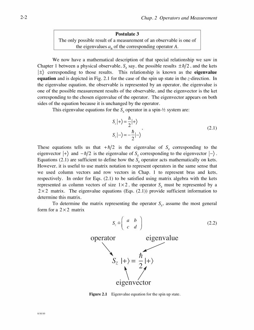
eigenvalue
eigenvector
operator
Sz |+Ú =—2 |+Ú
Figure 2.1 Eigenvalue equation for the spin up state.
Chap. 2 Operators and Measurement
8/10/10
2-3
where we are again using the ! symbol to mean "is represented by." Now write the
eigenvalue equations in matrix form:
a b
c d
!
"#$
%&1
0
!
"#$
%&= +!
2
1
0
!
"#$
%&
a b
c d
!
"#$
%&0
1
!
"#$
%&= '!
2
0
1
!
"#$
%&
. (2.3)
Note that we are still using the convention that the ± kets are used as the basis for the
representation. It is crucial that the rows and columns of the operator matrix are ordered
in the same manner as used for the ket column vectors; anything else would amount to
nonsense. An explicit labeling of the rows and columns of the operator and the basis kets
makes this clear:
Sz
+ !
+ a b
! c d
!!!!!!!!!!
+
+ 1
! 0
!!!!!!!!!!
!
+ 0
! 1
(2.4)
Carrying through the multiplication in Eqs. (2.3) yields
a
c
!
"#$
%&= +!
2
1
0
!
"#$
%&
b
d
!
"#$
%&= '!
2
0
1
!
"#$
%&
, (2.5)
which results in
a = +!
2 b = 0
c = 0 d = !!
2
. (2.6)
Thus the matrix representation of the operator Sz is
Sz!" 2 0
0 !" 2
"
#$$
%
&''
!"
2
1 0
0 !1"
#$%
&'
. (2.7)
Note two important features of this matrix: (1) it is a diagonal matrix—it has only
diagonal elements—and (2) the diagonal elements are the eigenvalues of the operator,
ordered in the same manner as the corresponding eigenvectors. In this example, the basis
used for the matrix representation is that formed by the eigenvectors ± of the operator
Chap. 2 Operators and Measurement
8/10/10
2-4
Sz. That the matrix representation of the operator in this case is a diagonal matrix is a
necessary and general result of linear algebra that will prove valuable as we study
quantum mechanics. In simple terms, we say that an operator is always diagonal in its
own basis. This special form of the matrix representing the operator is similar to the
special form that the eigenvectors ± take in this same representation—the eigenvectors
are unit vectors in their own basis. These ideas cannot be overemphasized, so we repeat
them:
An operator is always diagonal in its own basis.
Eigenvectors are unit vectors in their own basis.
Let's also summarize the matrix representations of the Sz operator and its
eigenvectors:
Sz!"
2
1 0
0 !1"
#$%
&'!!!!!!! + !
1
0
"
#$%
&'!!!!!!! ! ! 0
1
"
#$%
&'. (2.8)
2.1.1 Matrix Representation of Operators
Now consider how matrix representation works in general. Consider a general
operator A describing a physical observable (still in the two-dimensional spin-1/2
system), which we represent by the general matrix
A !a b
c d
!
"#$
%& (2.9)
in the Sz basis. The operation of A on the basis ket + yields
A + !a b
c d
!
"#$
%&1
0
!
"#$
%&=
a
c
!
"#$
%&. (2.10)
The inner product of this new ket A + with the ket + (converted to a bra following the
rules) results in
+ A + = 1 0( ) a
c
!
"#$
%&= a . (2.11)
Chap. 2 Operators and Measurement
8/10/10
2-5
HaLbra ket
operatorXf»A»y\
‚bra |OPERATOR|ketÚ
HbLrow column
operatorXn»A»m\
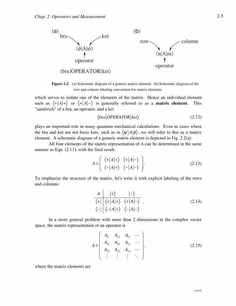
Figure 2.2 (a) Schematic diagram of a generic matrix element. (b) Schematic diagram of the
row and column labeling convention for matrix elements.
which serves to isolate one of the elements of the matrix. Hence an individual element
such as + A + or + A ! is generally referred to as a matrix element. This
"sandwich" of a bra, an operator, and a ket
bra OPERATOR ket (2.12)
plays an important role in many quantum mechanical calculations. Even in cases where
the bra and ket are not basis kets, such as in ! A " , we still refer to this as a matrix
element. A schematic diagram of a generic matrix element is depicted in Fig. 2.2(a).
All four elements of the matrix representation of A can be determined in the same
manner as Eqn. (2.11), with the final result
A !+ A + + A !
! A + ! A !
"
#$$
%
&''
. (2.13)
To emphasize the structure of the matrix, let's write it with explicit labeling of the rows
and columns:
A + !
+ + A + + A !
! ! A + ! A !
. (2.14)
In a more general problem with more than 2 dimensions in the complex vector
space, the matrix representation of an operator is
A !
A11
A12
A13"
A21
A22
A23"
A31
A32
A33"
# # # $
!
"
####
$
%
&&&&
, (2.15)
where the matrix elements are
Chap. 2 Operators and Measurement
8/10/10
2-6
Aij = i A j (2.16)
and the basis is assumed to be the states labeled i , with the subscripts i and j labeling
the rows and columns respectively, as depicted in Fig. 2.2(b). Using this matrix
representation, the action of this operator on a general ket ! = cii
i
" is
A ! !
A11
A12
A13"
A21
A22
A23"
A31
A32
A33"
# # # $
"
#
$$$$
%
&
''''
c1
c2
c3
#
"
#
$$$$
%
&
''''
=
A11c1+ A
12c2+ A
13c3+"
A21c1+ A
22c2+ A
23c3+"
A31c1+ A
32c2+ A
33c3+"
#
"
#
$$$$
%
&
''''
. (2.17)
If we write the new ket ! = A " as ! = bii
i
" , then from Eqn. (2.17) the
coefficients bi are
bi = Aijj
! cj (2.18)
in summation notation.
2.1.2 Diagonalization of Operators
In the case of the operator Sz above, we used the experimental results and the
eigenvalue equations to find the matrix representation of the operator in Eqn. (2.7). It is
more common to work the other way. That is, one is given the matrix representation of
an operator and is asked to find the possible results of a measurement of the
corresponding observable. According to the 3rd postulate, the possible results are the
eigenvalues of the operator, and the eigenvectors are the quantum states representing
them. In the case of a general operator A in a two-state system, the eigenvalue equation
is
A an= a
nan
, (2.19)
where we have labeled the eigenvalues an
and we have labeled the eigenvectors with the
corresponding eigenvalues. In matrix notation, the eigenvalue equation is
A11
A12
A21
A22
!
"##
$
%&&
cn1
cn2
!
"##
$
%&&= a
n
cn1
cn2
!
"##
$
%&&
, (2.20)
where cn1
and cn2
are the unknown coefficients of the eigenvector an
corresponding to
the eigenvalue an
. This matrix equation yields the set of homogeneous equations
A11! a
n( )cn1 + A12cn2 = 0
A21cn1+ A
22! a
n( )cn2 = 0. (2.21)
The rules of linear algebra dictate that a set of homogeneous equations has solutions for
the unknowns cn1
and cn2
only if the determinant of the coefficients vanishes:
Chap. 2 Operators and Measurement
8/10/10
2-7
A11! a
nA12
A21
A22! a
n
= 0 . (2.22)
It is common notation to use the symbol ! for the eigenvalues, in which case this
equation is
det A ! "I( ) = 0 , (2.23)
where I is the identity matrix
I =1 0
0 1
!
"#$
%&. (2.24)
Equation (2.23) is known as the secular or characteristic equation. It is a second order
equation in the parameter ! and the two roots are identified as the two eigenvalues a1 and
a2 that we are trying to find. Once these eigenvalues are found, they are then individually
substituted back into Eqs. (2.21), which are solved to find the coefficients of the
corresponding eigenvector.
Example 2.1
Assume that we know (e.g., from Problem 2.1) that the matrix representation for
the operator Sy is
Sy !"
2
0 !ii 0
"
#$%
&' (2.25)
Find the eigenvalues and eigenvectors of the operator Sy.
The general eigenvalue equation is
Sy ! = ! ! , (2.26)
and the possible eigenvalues ! are found using the secular equation
det Sy ! "I = 0 . (2.27)
The secular equation is
!" !i!
2
i!
2!"
= 0 . (2.28)
and solving yields the eigenvalues
Chap. 2 Operators and Measurement
8/10/10
2-8
!2 + i2!
2
"#$
%&'2
= 0
!2 (!
2
"#$
%&'2
= 0
!2 =!
2
"#$
%&'2
! = ±!
2
, (2.29)
which was to be expected, because we know that the only possible results of a
measurement of any spin component are ±! 2 .
As before, we label the eigenvectors ±y. The eigenvalue equation for the
positive eigenvalue is
Sy + y= +!
2+
y, (2.30)
or in matrix notation
!
2
0 !ii 0
"
#$%
&'a
b
"
#$%
&'= +!
2
a
b
"
#$%
&', (2.31)
where we must solve for a and b to determine the eigenvector. Multiplying through and
canceling the common factor yields
!ibia
"
#$%
&'=
a
b
"
#$%
&'. (2.32)
This results in two equations, but they are not linearly independent, so we need some
more information. The normalization condition provides what we need. Thus we have 2
equations that determine the eigenvector coefficients:
b = ia
a2
+ b2
= 1. (2.33)
Solving these yields
a2
+ ia2
= 1
a2
=1
2
. (2.34)
Again we follow the convention of choosing the first coefficient to be real and positive,
resulting in
a =
1
2
b = i1
2
. (2.35)
Chap. 2 Operators and Measurement
8/10/10
2-9
Thus the eigenvector corresponding to the positive eigenvalue is
+y!
1
2
1
i
!
"#$
%&. (2.36)
Likewise, one can find the eigenvector for the negative eigenvalue to be
!y!
1
2
1
!i"
#$%
&'. (2.37)
These are, of course, the same states we found in Chapter 1 (Eqn. 1.57).
This procedure of finding the eigenvalues and eigenvectors of a matrix is known
as diagonalization of the matrix and is the key step in many quantum mechanics
problems. Generally if we find a new operator, the first thing we do is diagonalize it to
find its eigenvalues and eigenvectors. However, we stop short of the mathematical
exercise of finding the matrix that transforms the original matrix to its new diagonal
form. This would amount to a change of basis from the original basis to a new basis of
the eigenvectors we have just found, much like a rotation in three dimensions changes
from one coordinate system to another. We don’t want to make this change of basis. In
the example above, the Sy matrix is not diagonal, whereas the Sz matrix is diagonal,
because we are using the Sz basis. It is common practice to use the Sz basis as the default
basis, so you can assume that is the case unless you are told otherwise.
In summary, we now know three operators and their eigenvalues and
eigenvectors. The spin component operators Sx, Sy, and Sz all have eigenvalues ±! 2 .
The matrix representations of the operators and eigenvectors are (see Problem 2.1)
Sx !"
2
0 1
1 0
!
"#$
%&!!!!!!! +
x!1
2
1
1
!
"#$
%&!!!!!!! '
x!1
2
1
'1!
"#$
%&
Sy !"
2
0 'ii 0
!
"#$
%&!!!!!! +
y!1
2
1
i
!
"#$
%&!!!!!!! '
y!1
2
1
'i!
"#$
%&
Sz !"
2
1 0
0 '1!
"#$
%&!!!!!! + !
1
0
!
"#$
%&!!!!!!!!!!!!!!! ' ! 0
1
!
"#$
%&
. (2.38)
2.2 New Operators
2.2.1 Spin Component in General Direction
Now that we know the three operators corresponding to the spin components
along the three Cartesian axes, we can use them to find the operator Sn for the spin
component along a general direction n . This new operator will allow us to predict
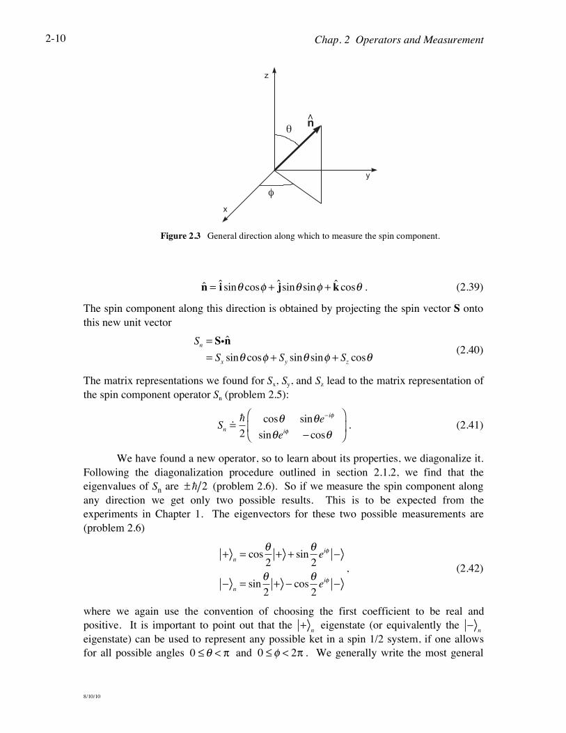
results of experiments we have not yet performed. The direction n is specified by the
polar and azimuthal angles ! and " as shown in Fig. 2.3. The unit vector n is
Chap. 2 Operators and Measurement
8/10/10
2-10
!
" n#
Figure 2.3 General direction along which to measure the spin component.
n = i sin! cos" + jsin! sin" + kcos! . (2.39)
The spin component along this direction is obtained by projecting the spin vector S onto
this new unit vector
Sn = Sin
= Sx sin! cos" + Sy sin! sin" + Sz cos! (2.40)
The matrix representations we found for Sx, Sy, and Sz lead to the matrix representation of
the spin component operator Sn (problem 2.5):
Sn!"
2
cos! sin!e" i#
sin!ei# " cos!
$
%&
'
() . (2.41)
We have found a new operator, so to learn about its properties, we diagonalize it.
Following the diagonalization procedure outlined in section 2.1.2, we find that the
eigenvalues of Sn are ±! 2 (problem 2.6). So if we measure the spin component along
any direction we get only two possible results. This is to be expected from the
experiments in Chapter 1. The eigenvectors for these two possible measurements are
(problem 2.6)
+n= cos
!
2+ + sin
!
2ei" #
#n= sin
!
2+ # cos
!
2ei" #
, (2.42)
where we again use the convention of choosing the first coefficient to be real and
positive. It is important to point out that the +n
eigenstate (or equivalently the !n
eigenstate) can be used to represent any possible ket in a spin 1/2 system, if one allows
for all possible angles 0 !" < # and 0 !" < 2# . We generally write the most general
Chap. 2 Operators and Measurement
8/10/10
2-11
state as ! = a + + b " , where a and b are complex. Requiring that the state be
normalized and using the freedom to choose the first coefficient real and positive reduces
this to
! = a + + 1" a2
ei# " . (2.43)
If we change the parametrization of a to cos ! 2( ) , we see that +n
is equivalent to the
most general state ! . This correspondence between the +n
eigenstate and the most
general state is only valid in a two-state system such as spin 1/2. In systems with more
dimensionality, it does not hold because more parameters are needed to specify the most
general state than are afforded by the two angles ! and ".
Example 2.2
Find the probabilities of the measurements shown in Fig. 2.4, assuming that the 1st
Stern-Gerlach analyzer is aligned along the direction n defined by the angles ! = 2" 3
and ! = " 4 .
The measurement by the 1st Stern-Gerlach analyzer prepares the system in the
spin up state +n
along the direction n . This state is then the input state to the 2nd Stern-
Gerlach analyzer. The input state is
!in
= +n= cos
"
2+ + sin
"
2ei# $
= cos%
3+ + sin
%
3ei% 4 $
=1
2+ !+!
3
2ei% 4 $
, (2.44)
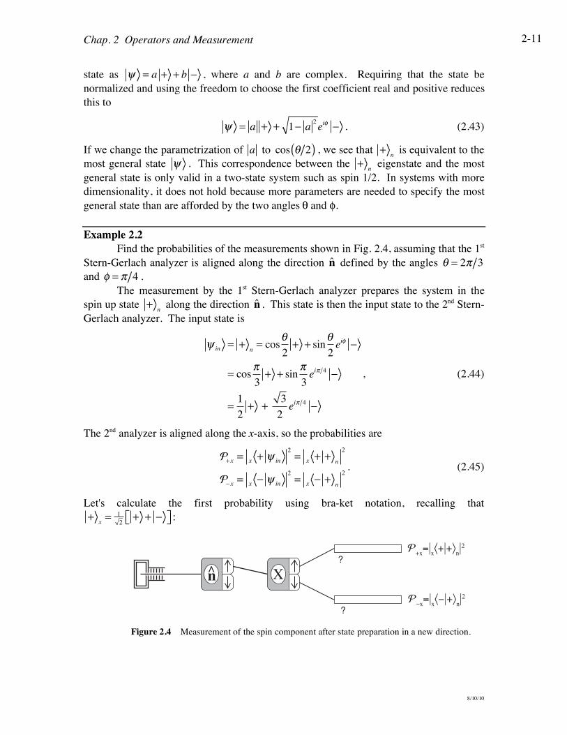
The 2nd analyzer is aligned along the x-axis, so the probabilities are
!+ x=
x+ !
in
2
=x+ +
n
2
!" x = x" !
in
2
=x" +
n
2. (2.45)
Let's calculate the first probability using bra-ket notation, recalling that
+x=
1
2+ + !"# $% :
X?
?
n!+x=|x$+|+%n|
2
!!x=|x$&|+%n|2
Figure 2.4 Measurement of the spin component after state preparation in a new direction.
Chap. 2 Operators and Measurement
8/10/10
2-12
!+ x=
x+ +
n
2
= 1
2+ + !"# $%
1
2+ + 3e
i& 4 !"#
$%
2
= 1
2 21+ 3e
i& 4"#
$%
2
= 1
81+ 3e
i& 4"#
$% 1+ 3e
! i& 4"#
$%
= 1
81+ 3 e
i& 4+ e
! i& 4( ) + 3"#
$%
= 1
84 + 2 3cos & 4( )"#
$%
= 1
84 + 2 3 2"#
$% ' 0.806
. (2.46)
Let's calculate the second probability using matrix notation, recalling that
!x=
1
2+ ! !"# $% :
!! x = x! +
n
2
= 1
21 !1( ) 1
2
1
3ei" 4
#
$%
&
'(
2
= 1
2 21! 3e
i" 4)* +,2
= 1
84 ! 2 3 cos " 4( ))* +,
= 1
84 ! 2 3 2)* +, - 0.194
. (2.47)
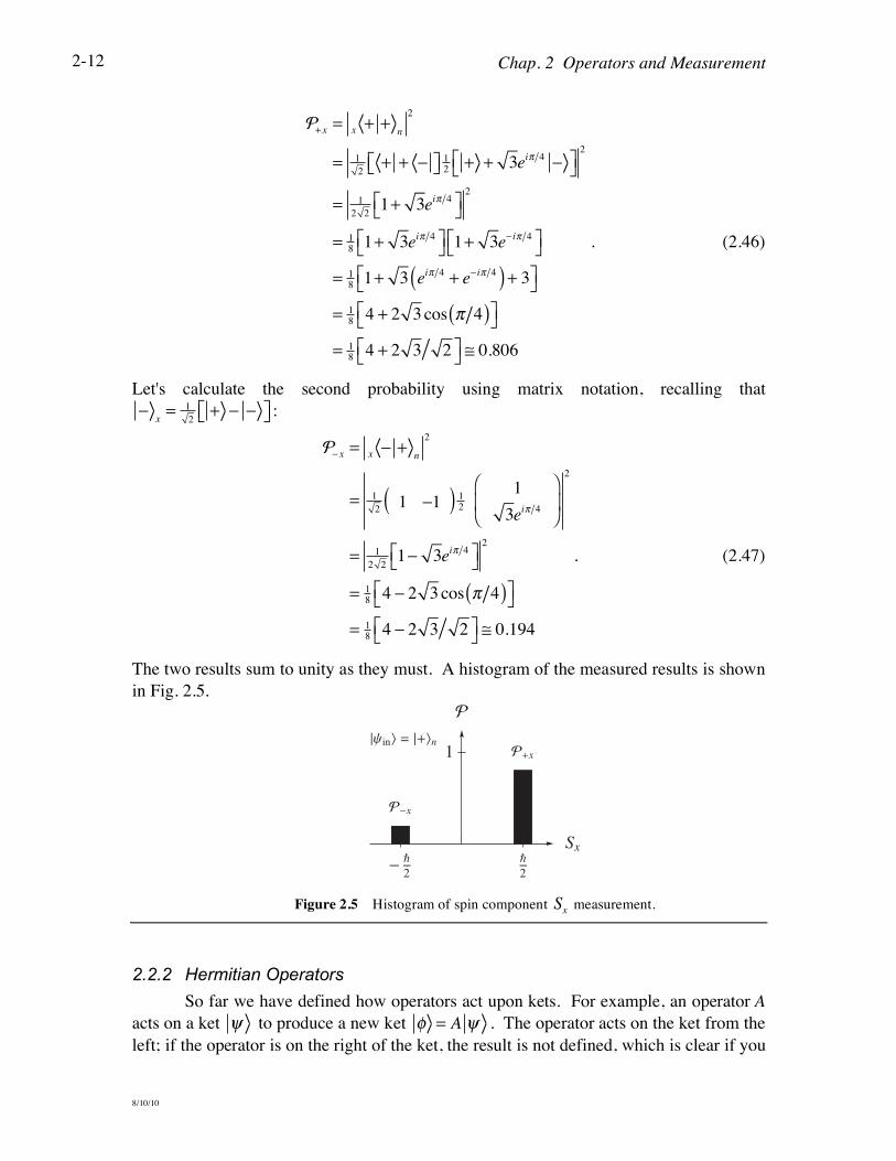
The two results sum to unity as they must. A histogram of the measured results is shown
in Fig. 2.5.
- —2
—2
Sx
1
!
!-x
!+x†yin\ = †+\n
Figure 2.5 Histogram of spin component Sx
measurement.
2.2.2 Hermitian Operators
So far we have defined how operators act upon kets. For example, an operator A
acts on a ket ! to produce a new ket ! = A " . The operator acts on the ket from the
left; if the operator is on the right of the ket, the result is not defined, which is clear if you
Chap. 2 Operators and Measurement
8/10/10
2-13
try to use matrix representation. Similarly, an operator acting on a bra must be on the
right side of the bra
! = " A (2.48)
and the result is another bra. However, the bra ! = " A is not the bra ! that
corresponds to the ket ! = A " . Rather the bra ! is found by defining a new
operator A† that obeys
! = " A† . (2.49)
This new operator A† is called the Hermitian adjoint of the operator A. We can learn
something about the Hermitian adjoint by taking the inner product of the state ! = A "
with another (unspecified) state !
! " = " ! *
# A+$% &' " = " A #$% &'{ }
*
# A+ " = " A #
*
, (2.50)
which relates the matrix elements of A and A†. Equation (2.50) tells us that the matrix
representing the Hermitian adjoint A† is found by transposing and complex conjugating
the matrix representing A. This is consistent with the definition of Hermitian adjoint used
in matrix algebra.
An operator A is said to be Hermitian if it is equal to its Hermitian adjoint A†. If
an operator is Hermitian, then the bra ! A is equal to the bra ! that corresponds to the
ket ! = A " . That is, a Hermitian operator can act to the right on a ket or to the left on
a bra with the same result. In quantum mechanics, all operators that correspond to
physical observables are Hermitian. This includes the spin operators we have already
encountered as well as the energy, position, and momentum operators that we will
introduce in later chapters. The Hermiticity of physical observables is important in light
of two features of Hermitian matrices. (1) Hermitian matrices have real eigenvalues,
which ensures that results of measurements are always real. (2) The eigenvectors of a
Hermitian matrix comprise a complete set of basis states, which ensures that we can use
the eigenvectors of any observable as a valid basis.
2.2.3 Projection Operators
For the spin-1/2 system, we now know four operators: Sx, Sy, Sz, and Sn. Let's
look for some other operators. Consider the ket ! written in terms of its coefficients in
the Sz basis
! = a + + b "
= + !( ) + + " !( ) ". (2.51)
Looking for the moment only at the first term, we can write it as a number times a ket, or
as a ket times a number:
Chap. 2 Operators and Measurement
8/10/10
2-14
+ !( ) + = + + !( ) (2.52)
without changing its meaning. Using the second form, we can separate the bra and ket
that form the inner product and obtain
+ + !( ) = + +( ) ! (2.53)
The term in parentheses is a product of a ket and a bra, but in the opposite order
compared to the inner product defined earlier. This new object must be an operator
because it acts on the ket ! and produces another ket: + !( ) + . This new type of
operator is known as an outer product.
Returning now to Eqn. (2.51), we write ! using these new operators:
! = + ! + + " ! "
= + + ! + " " !
= + + + " "( ) !
. (2.54)
The term in parentheses is a sum of two outer products, and is clearly an operator because
it acts on a ket to produce another ket. In this special case, the result is the same as the
original ket, so the operator must be the identity operator 1. This relationship is often
written as
+ + + ! ! = 1 , (2.55)
and is known as the completeness relation or closure. It expresses the fact that the basis
states ± comprise a complete set of states, meaning any arbitrary ket can be written in
terms of them. To make it obvious that outer products are operators, it is useful to
express Eqn. (2.55) in matrix notation using the standard rules of matrix multiplication:
+ + + ! ! !1
0
"
#$%
&'1 0( ) + 0
1
"
#$%
&'0 1( )
!1 0
0 0
"
#$%
&'+
0 0
0 1
"
#$%
&'
!1 0
0 1
"
#$%
&'
, (2.56)
Each outer product is represented by a matrix, as we expect for operators, and the sum of
these two outer products is represented by the identity matrix, which we expected from
Eqn. (2.54).
Now consider the individual operators + + and ! ! . These operators are
called projection operators, and for spin 1/2 they are given by
Chap. 2 Operators and Measurement
8/10/10
2-15
P+= + + !
1 0
0 0
!
"#$
%&
P' = ' ' ! 0 0
0 1
!
"#$
%&
. (2.57)
In terms of these new operators the completeness relation can also be written as
P++ P
!= 1 . (2.58)
When a projection operator for a particular eigenstate acts on a state ! , it produces a
new ket that is aligned along the eigenstate and has a magnitude equal to the amplitude
(including the phase) for the state ! to be in that eigenstate. For example,
P+! = + + ! = + !( ) +
P" ! = " " ! = " !( ) ". (2.59)
Note also that a projector acting on its corresponding eigenstate results in that eigenstate,
and a projector acting on an orthogonal state results in zero:
P++ = + + + = +
P!+ = ! ! + = 0
. (2.60)
Because the projection operator produces the probability amplitude, we expect that it
must be intimately tied to measurement in quantum mechanics.
We found in Chap. 1 that the probability of a measurement is given by the square
of the inner product of initial and final states (postulate 4). Using the new projection
operators, we rewrite the probability as
!+= + !
2
= + !*
+ !
= ! + + !
= ! P+!
. (2.61)
Thus we say that the probability of the measurement Sz= ! 2 can be calculated as a
matrix element of the projection operator, using the input state ! and the projector P+
corresponding to the result.
The other important aspect of quantum measurement that we learned in Chap. 1
was that a measurement disturbs the system. That is, if an input state ! is measured to
have Sz= +! 2 , then the output state is no longer ! , but is changed to + . We saw
above that the projection operator does this operation for us, with a multiplicative
constant of the probability amplitude. Thus if we divide by this amplitude, which is the
square root of the probability, then we can describe the abrupt change of the input state as
Chap. 2 Operators and Measurement
8/10/10
2-16
!" =P+"
" P+"
= + , (2.62)
where !" is the output state. This effect is described by the fifth postulate, which is
presented below and is often referred to as the projection postulate.
Postulate 5
After a measurement of A that yields the result an, the quantum system
is in a new state that is the normalized projection of the original
system ket onto the ket (or kets) corresponding to the result of the
measurement:
!" =Pn"
" Pn"
.
The projection postulate is at the heart of quantum measurement. This effect is
often referred to as the collapse (or reduction or projection) of the quantum state vector.
The projection postulate clearly states that quantum measurements cannot be made
without disturbing the system (except in the case where the input state is the same as the
output state), in sharp contrast to classical measurements. The collapse of the quantum
state makes quantum mechanics irreversible, again in contrast to classical mechanics.
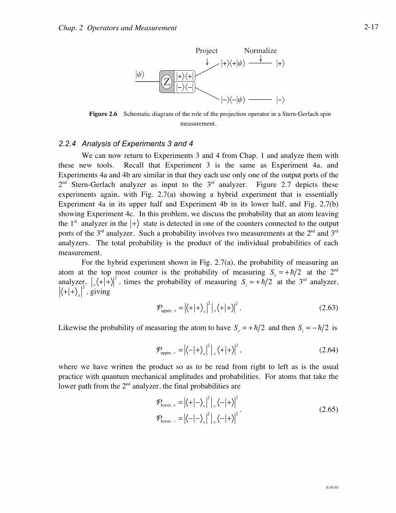
We can use the projection postulate to make a model of quantum measurement, as
shown in the revised depiction of a Stern-Gerlach measurement system in Fig. 2.6. The
projection operators act on the input state to produce output states with probabilities
given by the squares of the amplitudes that the projection operations yield. For example,
the input state !in
is acted on the projection operator P+= + + , producing an output
ket !out
= + + !in( ) with probability
!+= + !
in
2
. The output ket
!out
= + + !in( ) is really just a + ket that is not properly normalized, so we
normalize it for use in any further calculations. We do not really know what is going on
in the measurement process, so we cannot explain the mechanism of the collapse of the
quantum state vector. This lack of understanding makes some people uncomfortable with
this aspect of quantum mechanics, and has been the source of much controversy
surrounding quantum mechanics. Trying to better understand the measurement process
in quantum mechanics is an ongoing research problem. However, despite our lack of
understanding, the theory for predicting the results of experiments has been proven with
very high accuracy.
Chap. 2 Operators and Measurement
8/10/10
2-17
|y% Z |+%$+||&%$&|
|+%$+|y%
|&%$&|y%
|+%
|&%
Project Normalize' '
Figure 2.6 Schematic diagram of the role of the projection operator in a Stern-Gerlach spin
measurement.
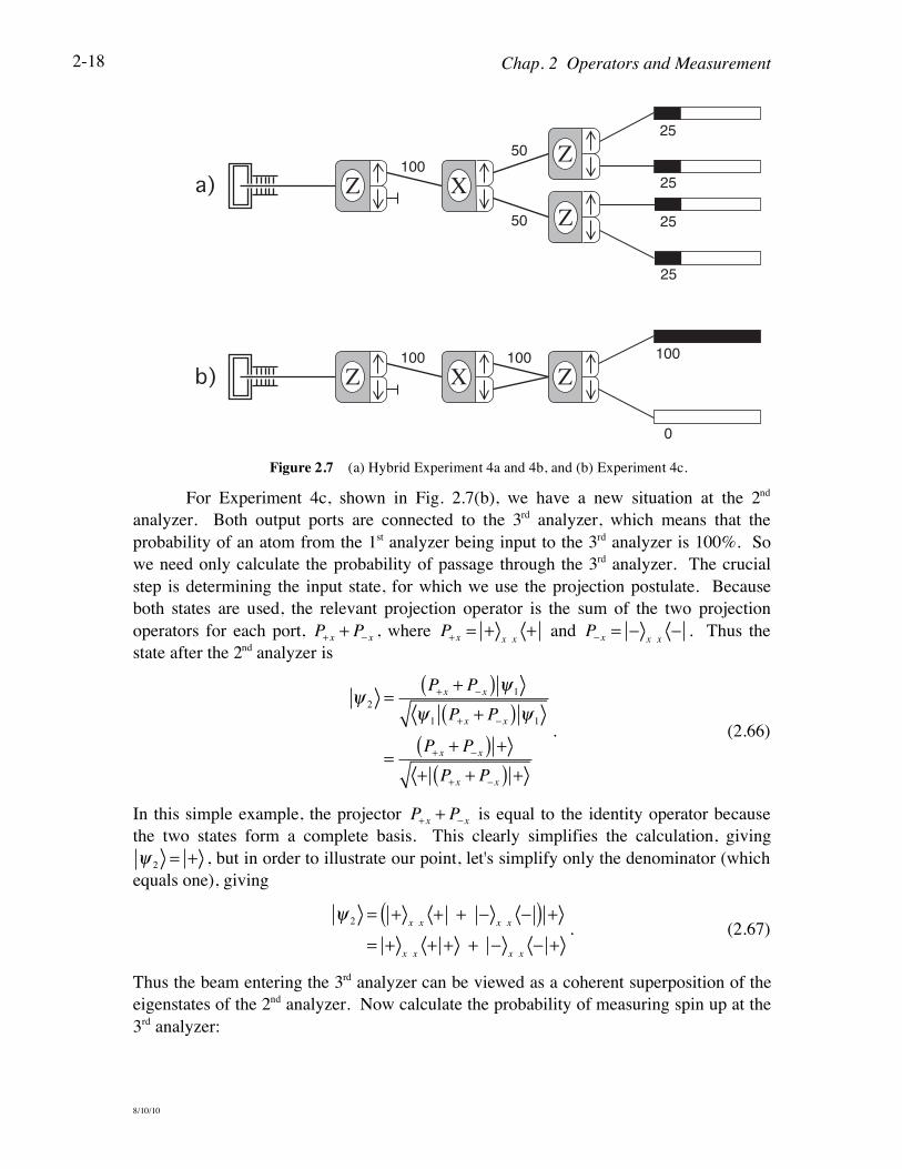
2.2.4 Analysis of Experiments 3 and 4
We can now return to Experiments 3 and 4 from Chap. 1 and analyze them with
these new tools. Recall that Experiment 3 is the same as Experiment 4a, and
Experiments 4a and 4b are similar in that they each use only one of the output ports of the
2nd Stern-Gerlach analyzer as input to the 3rd analyzer. Figure 2.7 depicts these
experiments again, with Fig. 2.7(a) showing a hybrid experiment that is essentially
Experiment 4a in its upper half and Experiment 4b in its lower half, and Fig. 2.7(b)
showing Experiment 4c. In this problem, we discuss the probability that an atom leaving
the 1st analyzer in the + state is detected in one of the counters connected to the output
ports of the 3rd analyzer. Such a probability involves two measurements at the 2nd and 3rd
analyzers. The total probability is the product of the individual probabilities of each
measurement.
For the hybrid experiment shown in Fig. 2.7(a), the probability of measuring an
atom at the top most counter is the probability of measuring Sx= +! 2 at the 2nd
analyzer, x+ +
2
, times the probability of measuring Sz= +! 2 at the 3rd analyzer,
+ +x
2
, giving
!upper, + = + +
x
2
x+ +
2
. (2.63)
Likewise the probability of measuring the atom to have Sx= +! 2 and then S
z= !! 2 is
!upper, ! = ! +
x
2
x+ +
2
, (2.64)
where we have written the product so as to be read from right to left as is the usual
practice with quantum mechanical amplitudes and probabilities. For atoms that take the
lower path from the 2nd analyzer, the final probabilities are
!lower, +
= + !x
2
x! +
2
!lower, !
= ! !x
2
x! +
2. (2.65)
Chap. 2 Operators and Measurement
8/10/10
2-18
100
0
XZ Z100 100
25
25Z
XZ100
50
25
25
Z50
Figure 2.7 (a) Hybrid Experiment 4a and 4b, and (b) Experiment 4c.
For Experiment 4c, shown in Fig. 2.7(b), we have a new situation at the 2nd
analyzer. Both output ports are connected to the 3rd analyzer, which means that the
probability of an atom from the 1st analyzer being input to the 3rd analyzer is 100%. So
we need only calculate the probability of passage through the 3rd analyzer. The crucial
step is determining the input state, for which we use the projection postulate. Because
both states are used, the relevant projection operator is the sum of the two projection
operators for each port, P+ x+ P
! x, where P
+ x= +
x x+ and P
! x= !
x x! . Thus the
state after the 2nd analyzer is
!2=
P+ x+ P" x( ) ! 1
!1P+ x+ P" x( ) ! 1
=P+ x+ P" x( ) +
+ P+ x+ P" x( ) +
. (2.66)
In this simple example, the projector P+ x+ P
! x is equal to the identity operator because
the two states form a complete basis. This clearly simplifies the calculation, giving
!2= + , but in order to illustrate our point, let's simplify only the denominator (which
equals one), giving
!2= +
x x+ + "
x x"( ) +
= +x x
+ + + "x x
" +. (2.67)
Thus the beam entering the 3rd analyzer can be viewed as a coherent superposition of the
eigenstates of the 2nd analyzer. Now calculate the probability of measuring spin up at the
3rd analyzer:
Chap. 2 Operators and Measurement
8/10/10
2-19
!+= + !
2
2
= + +x x
+ + + + "x x
" +2
. (2.68)
The probability of measuring spin down at the 3rd analyzer is similarly
!! = ! "2
2
= ! +x x
+ + + ! !x x
! +2
. (2.69)
In each case, the probability is a square of a sum of amplitudes, each amplitude being the
amplitude for a successive pair of measurements. For example, in !!
the amplitude
! +x x
+ + refers to the upper path that the initial + state takes as it is first measured
to be in the +x state, and then measured to be in the ! state (read from right to left).
This amplitude is added to the amplitude for the lower path because the beams of the 2nd
analyzer are combined, in the proper fashion, to create the input beam to the 3rd analyzer.
When the sum of amplitudes is squared, four terms are obtained, two squares and two
cross terms, giving
!!= ! +
x x+ +
2
+ ! !x x
! +2
+ ! +x
*
x+ +
*! !
x x! +
+ ! +x x
+ + ! !x
*
x! +
*
= !upper, ! + !lower, ! + interference terms
. (2.70)
This tells us that the probability of detecting an atom to have spin down when both paths
are used is the sum of the probabilities for detecting a spin down atom when either the
upper path or the lower path is used alone plus additional cross terms involving both
amplitudes, which are commonly called interference terms. It is these additional terms,
which are not complex squares and so could be positive or negative, that allow the total
probability to become zero in this case, illustrating the phenomenon of interference.
This interference arises from the nature of the superposition of states that enters
the 3rd analyzer. To illustrate, consider what happens if we change the superposition state
to a mixed state as we discussed previously (Sec. 1.2.3). Recall that a superposition state
implies a beam with each atom in the same state, which is a combination of states, while
a mixed state implies that the beam consists of atoms in separate states. As we have
described it so far, Experiment 4c involves a superposition state as the input to the 3rd
analyzer. We can change this to a mixed state by "watching" to see which of the two
output ports of the 2nd analyzer each atom travels through. There are a variety of ways to
imagine doing this experimentally. The usual idea proposed is to illuminate the paths
with light and watch for the scattered light from the atoms. With proper design of the
optics, the light can be localized sufficiently to determine which path the atom takes.
Hence, such experiments are generally referred to as "Which Path" or "Welcher Weg"
experiments. Such experiments can be performed in the SPINS program by selecting the
Chap. 2 Operators and Measurement
8/10/10
2-20
"Watch" feature. Once we know which path the atom takes, the state is not the
superposition !2
described above, but is either +x or !
x, depending on which path
produces the light signal. To find the probability that atoms are detected at the spin down
counter of the 3rd analyzer, we add the probabilities for atoms to follow the path
+ ! +x! " to the probability for other atoms to follow the path + ! "
x! "
because these are independent events, giving
!watch, ! = ! +
x x+ +
2
+ ! !x x
! +2
= !upper, ! + !lower, !
, (2.71)
in which no interference terms are present.
This interference example illustrates again the important distinction between a
coherent superposition state and a statistical mixed state. In a coherent superposition,
there is a definite relative phase between the different states, which gives rise to
interference effects that are dependent on that phase. In a statistical mixed state, the
phase relationship between the states has been destroyed and the interference is washed
out. Now we can understand what it takes to have the beams "properly" combined after
the 2nd analyzer of Experiment 4c. The relative phases of the two paths must be
preserved. Anything that randomizes the phase is equivalent to destroying the
superposition and leaving only a statistical mixture. If the beams are properly combined
to leave the superposition intact, the results of Experiment 4c are the same as if no
measurement were made at the 2nd analyzer. So even though we have used a measuring
device in the middle of Experiment 4c, we generally say that no measurement was made
there. We can summarize our conclusions by saying that if no measurement is made at
the intermediate state, then we add amplitudes and then square to find the probability,
while if an intermediate measurement is performed (i.e., watching), then we square the
amplitudes first and then add to find the probability. One is the square of a sum and the
other is the sum of squares, and only the former exhibits interference.
2.3 Measurement
Lets' discuss how the probabilistic nature of quantum mechanics affects the way
experiments are performed and compared with theory. In classical physics, a theoretical
prediction can be reliably compared to a single experimental result. For example, a
prediction of the range of a projectile can be tested by doing an experiment. The
experiment may be repeated several times in order to understand and possibly reduce any
systematic errors (e.g., wind) and measurement errors (e.g., misreading the tape
measure). In quantum mechanics, a single measurement is meaningless. If we measure
an atom to have spin up in a Stern-Gerlach analyzer, we cannot discern whether the
original state was + or !x or any arbitrary state ! (except ! ). Moreover, we
cannot repeat the measurement on the same atom, because the original measurement
changed the state, per the projection postulate.
Thus, one must, by necessity, perform identical measurements on identically
prepared systems. In the spin 1/2 example, an initial Stern-Gerlach analyzer is used to
Chap. 2 Operators and Measurement
8/10/10
2-21
prepare atoms in a particular state ! . Then a second Stern-Gerlach analyzer is used to
perform the same experiment on each identically prepared atom. Consider performing a
measurement of Sz on N identically prepared atoms. Let N+ be the number of times the
result +! 2 is recorded and N- be the number of times the result
!! 2 is recorded.
Because there are only two possible results for each measurement, we must have
N = N+ + N-. The probability postulate (postulate 4) predicts that the probability of
measuring +! 2 is
!+= + !
2
. (2.72)
For a finite number N of atoms, we expect that N+ is only approximately equal to !+ !N
due to the statistical fluctuations inherent in a random process. Only in the limit of an
infinite number N do we expect exact agreement:
limN!"
N+
N= !
+= + #
2
. (2.73)
It is useful to characterize a data set in terms of the mean and standard deviation
(see Appendix A for further information on probability). The mean value of a data set is
the average of all the measurements. The expected or predicted mean value of a
measurement is the sum of the products of each possible result and its probability, which
for this spin-! measurement is
Sz= +
!
2
!"#
$%&!+!!+!! '
!
2
!"#
$%&!' . (2.74)
where the angle brackets signify average or mean value. Using the rules of quantum
mechanics we rewrite this mean value as
Sz= +!
2+ !
2
!!+!! "!
2
#$%
&'(
" !2
= +!
2! + + ! !!+ ! "
!
2
#$%
&'(! " " !
= ! +!
2+ + ! !!+!! "
!
2
#$%
&'(" " !)
*+,
-.
= ! Sz+ + ! !!+!!S
z" " !)* ,-
= ! Sz
+ + !!+!! " ")* ,- !
. (2.75)
According to the completeness relation, the term in square brackets in the last line is
unity, so we obtain
Sz= ! S
z! . (2.76)
We now have two ways to calculate the predicted mean value, Eqn. (2.74) and
Eqn. (2.76). Which you use generally depends on what quantities you have readily
Chap. 2 Operators and Measurement
8/10/10
2-22
available. The matrix element version in Eqn. (2.76) is more common and is especially
useful in systems that are more complicated than the 2-level spin-! system. This
predicted mean value is commonly called the expectation value, but it is not the
expected value of any single experiment. Rather it is the expected mean value of a large
number of experiments. It is not a time average, but an average over many identical
experiments. For a general quantum mechanical observable, the expectation value is
A = ! A ! = an!an
n
" (2.77)
where an
are the eigenvalues of the operator A .
To see how the concept of expectation values applies to our study of spin-1/2
systems, consider two examples. First consider a system prepared in the state + . The
expectation value of Sz is
Sz= + S
z+ , (2.78)
which we calculate with bra-ket notation
Sz= + S
z+
= +!
2+
=!
2+ +
=!
2
. (2.79)
This result should seem obvious because +! 2 is the only possible result of a
measurement of Sz for the + state, so it must be the expectation value.
Next consider a system prepared in the state +x. In this case, the expectation
value of Sz is
Sz=
x+ S
z+
x. (2.80)
Using matrix notation, we obtain
Sz= 1
21 1( )
!
2
1 0
0 !1"
#$%
&'1
2
1
1
"
#$%
&'
=!
41 1( ) 1
!1"
#$%
&'= 0!
. (2.81)
Again this is what you expect, because the two possible measurement results ±! 2 each
have 50% probability, so the average value is zero. Note that the value of zero is never
measured, so it is not the value "expected" for any given measurement, but rather the
expected mean value of an ensemble of measurements.
Chap. 2 Operators and Measurement
8/10/10
2-23
In addition to the mean value, it is common to characterize a measurement by the
standard deviation, which quantifies the spread of measurements about the mean or
expectation value. The standard deviation is defined as the square root of the mean of
the square of the deviations from the mean, and for an observable A is given by
!A = A " A( )2
, (2.82)
where the angle brackets signify average value as used in the definition of an expectation
value. This result is also often called the root-mean-square deviation, or r.m.s.
deviation. We need to square the deviations because the deviations from the mean are
equally distributed above and below the mean in such a way that the average of the
deviations themselves is zero. This expression can be simplified by expanding the square
and performing the averages, resulting in
!A = A2" 2A A + A
2( )
= A2" 2 A A + A
2
= A2" A
2
, (2.83)
where one must be clear to distinguish between the square of the mean A2
and the
mean of the square A2
. While the mean of the square of an observable may not be a
common experimental quantity, it can be calculated using the definition of the
expectation value
A2= ! A
2 ! . (2.84)
The square of an operator means that the operator acts twice in succession:
A2 ! = AA ! = A A !( ) . (2.85)
To gain experience with the standard deviation, return to the two examples used
above. To calculate the standard deviation, we need to find the mean of the square of the
operator Sz. In the first case ( + initial state), we get
Sz
2= + S
z
2+ = + S
zSz+ = + S
z
!
2+
= +!
2
!"#
$%&2
+
=!
2
!"#
$%&2
. (2.86)
We already have the mean of the operator Sz in Eqn. (2.79) so the standard deviation is
Chap. 2 Operators and Measurement
8/10/10
2-24
!Sz= S
z
2 " Sz
2
=!
2
#$%
&'(2
"!
2
#$%
&'(2
= 0!
, (2.87)
which is to be expected because there is only one possible result, and hence no spread in
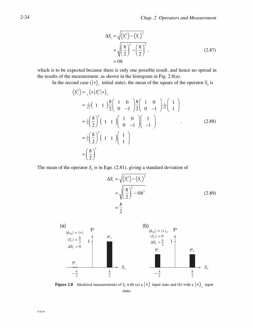
the results of the measurement, as shown in the histogram in Fig. 2.8(a).
In the second case ( +x initial state), the mean of the square of the operator Sz is
Sz
2=
x+ S
z
2+
x
= 1
21 1( )
!
2
1 0
0 !1"
#$%
&'!
2
1 0
0 !1"
#$%
&'1
2
1
1
"
#$%
&'
= 1
2
!
2
"#$
%&'2
1 1( ) 1 0
0 !1"
#$%
&'1
!1"
#$%
&'
= 1
2
!
2
"#$
%&'2
1 1( ) 1
1
"
#$%
&'
=!
2
"#$
%&'2
. (2.88)
The mean of the operator Sz is in Eqn. (2.81), giving a standard deviation of
!Sz= S
z
2 " Sz
2
=!
2
#$%
&'(2
" 0!2
=!
2
(2.89)
(a) (b)
- —2
—2
Sz
1
!
!-
!+
DSz = 0
†yin\ = †+\
- —2
—2
Sz
1
!
!- !+
XSz\ = 0†yin\ = †+\xXSz\ = —
2 DSz = —2
Figure 2.8 Idealized measurements of Sz with (a) a + input state and (b) with a +x
input
state.
Chap. 2 Operators and Measurement
8/10/10
2-25
Again this makes sense because each measurement deviates from the mean ( 0! ) by the
same value of ! 2 , as shown in the histogram in Fig. 2.8(b).
The standard deviation !A represents the uncertainty in the results of an
experiment. In quantum mechanics, this uncertainty is inherent and fundamental,
meaning that you cannot design the experiment any better to improve the result. What
we have calculated then, is the minimum uncertainty allowed by quantum mechanics.
Any actual uncertainty may be larger due to experimental error. This is another
ramification of the probabilistic nature of quantum mechanics and will lead us to the
Heisenberg uncertainty relation in Section 2.5.
2.4 Commuting Observables
We found in Experiment 3 that two incompatible observables could not be known
or measured simultaneously, because measurement of one somehow erased knowledge of
the other. Let us now explore further what it means for two observables to be
incompatible and how incompatibility affects the results of measurements. First we need
to define a new object called a commutator. The commutator of two operators is
defined as the difference between the products of the two operators taken in alternate
orders:
[A,B] = AB ! BA . (2.90)
If the commutator is equal to zero, we say that the operators or observables commute; if
it is not zero, we say they don't commute. Whether or not two operators commute has
important ramifications in analyzing a quantum system and in making measurements of
the two observables represented by those operators.
Consider what happens when two operators A and B do commute:
[A,B] = 0
AB ! BA = 0
AB = BA
. (2.91)
Thus for commuting operators, the order of operation does not matter, whereas it does for
noncommuting operators. Now let a be an eigenstate of the operator A with eigenvalue
a:
A a = a a . (2.92)
Operate on both sides of this equation with the operator B and use the fact that A and B
commute:
BA a = Ba a
AB a = aB a
A B a( ) = a B a( )
. (2.93)
The last equation says that the state B a is also an eigenstate of the operator A with the
same eigenvalue a. Assuming that each eigenvalue has a unique eigenstate (which is true
Chap. 2 Operators and Measurement
8/10/10
2-26
if there is no degeneracy, but we haven't discussed degeneracy yet), the state B a must
be some scalar multiple of the state a . If we call this multiple b, then we can write
B a = b a , (2.94)
which is just an eigenvalue equation for the operator B. Thus we must conclude that the
state a is also an eigenstate of the operator B, with the eigenvalue b. The assumption
that the operators A and B commute has led us to the result that A and B have common or
simultaneous sets of eigenstates. This result bears repeating:
Commuting operators share common eigenstates.
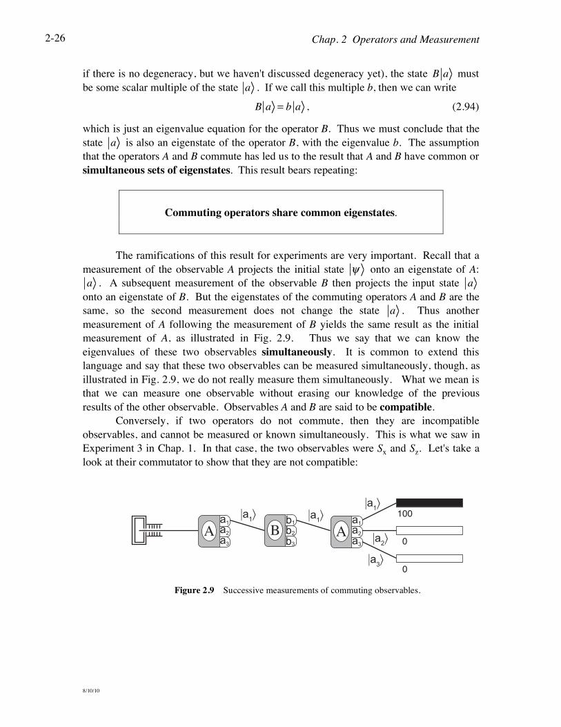
The ramifications of this result for experiments are very important. Recall that a
measurement of the observable A projects the initial state ! onto an eigenstate of A:
a . A subsequent measurement of the observable B then projects the input state a
onto an eigenstate of B. But the eigenstates of the commuting operators A and B are the
same, so the second measurement does not change the state a . Thus another
measurement of A following the measurement of B yields the same result as the initial
measurement of A, as illustrated in Fig. 2.9. Thus we say that we can know the
eigenvalues of these two observables simultaneously. It is common to extend this
language and say that these two observables can be measured simultaneously, though, as
illustrated in Fig. 2.9, we do not really measure them simultaneously. What we mean is
that we can measure one observable without erasing our knowledge of the previous
results of the other observable. Observables A and B are said to be compatible.
Conversely, if two operators do not commute, then they are incompatible
observables, and cannot be measured or known simultaneously. This is what we saw in
Experiment 3 in Chap. 1. In that case, the two observables were Sx and Sz. Let's take a
look at their commutator to show that they are not compatible:
100
0
0ABA
|a1% |a1%|a1%
|a2%
|a3%
Figure 2.9 Successive measurements of commuting observables.
Chap. 2 Operators and Measurement
8/10/10
2-27
[Sz ,Sx ] !"
2
1 0
0 !1
"
#$%
&'"
2
0 1
1 0
"
#$%
&'!!!!!"
2
0 1
1 0
"
#$%
&'"
2
1 0
0 !1
"
#$%
&'
!"
2
"#$
%&'
2
0 1
!1 0
"
#$%
&'! 0 !1
1 0
"
#$%
&'(
)**
+
,--
!"
2
"#$
%&'
2
0 2
!2 0
"
#$%
&'
= i"Sy
(2.95)
As expected, these two operators do not commute. In fact, none of the spin component
operators commute with each other. The complete commutation relations are
[Sx ,Sy ] = i!Sz
[Sy ,Sz ] = i!Sx
[Sz ,Sx ] = i!Sy
, (2.96)
so written to make the cyclic relations clear.
When we represent operators as matrices, we can often decide whether two
operators commute by inspection of the matrices. Recall the important statement: An
operator is always diagonal in its own basis. If you are presented with two matrices that
are both diagonal, they must share a common basis, and so they commute with each
other. To be explicit, the product of two diagonal matrices
AB !
a1
0 0 "
0 a2
0 "
0 0 a3"
# # # $
!
"
####
$
%
&&&&
b1
0 0 "
0 b2
0 "
0 0 b3"
# # # $
!
"
####
$
%
&&&&
!
a1b1
0 0 "
0 a2b2
0 "
0 0 a3b3"
# # # $
!
"
####
$
%
&&&&
, (2.97)
is clearly independent of the order of the product. Note, however, that you may not
conclude that two operators do not commute if one is diagonal and one is not, nor if both
are not diagonal.
2.5 Uncertainty Principle
The intimate connection between the commutator of two observables and the
possible precision of measurements of the two corresponding observables is reflected in
an important relation that we simply state here (see more advanced texts for a derivation).
Chap. 2 Operators and Measurement
8/10/10
2-28
The product of the uncertainties or standard deviations of two observables is related to
the commutator of the two observables:
!A!B "1
2[A,B] . (2.98)
This is the uncertainty principle of quantum mechanics. Consider what it says about a
simple Stern-Gerlach experiment. The uncertainty principle for the Sx and Sy spin
components is
!Sx!Sy "1
2[Sx ,Sy ]
"1
2i!Sz
"!
2Sz
. (2.99)
These uncertainties are the minimal quantum mechanical uncertainties that would arise in
any experiment. Any experimental uncertainties, due for example to experimenter error,
apparatus errors, and statistical limitations, would be additional.
Let's now apply the uncertainty principle to Experiment 3 where we first learned
of the impact of measurements in quantum mechanics. If the initial state is + , then a
measurement of Sz results in an expectation value Sz= ! 2 with an uncertainty
!Sz= 0 , as illustrated in Fig. 2.8(a). Thus the uncertainty principle dictates that the
product of the other uncertainties for measurements of the + state is
!Sx!Sy "!
2
#$%
&'(2
, (2.100)
or simply
!Sx!Sy " 0 . (2.101)
This implies that
!Sx " 0
!Sy " 0. (2.102)
The conclusion to draw from this is that while we can know one spin component
absolutely (!Sz= 0 ), we can never know all three, nor even two, simultaneously. This is
in agreement with our results from Experiment 3. This lack of ability to measure all spin
components simultaneously implies that the spin does not really point in a given
direction, as a classical spin or angular momentum does. So when we say that we have
measured "spin up," we really mean only that the spin component along that axis is up, as
opposed to down, and not that the complete spin angular momentum vector points up
along that axis.
Chap. 2 Operators and Measurement
8/10/10
2-29
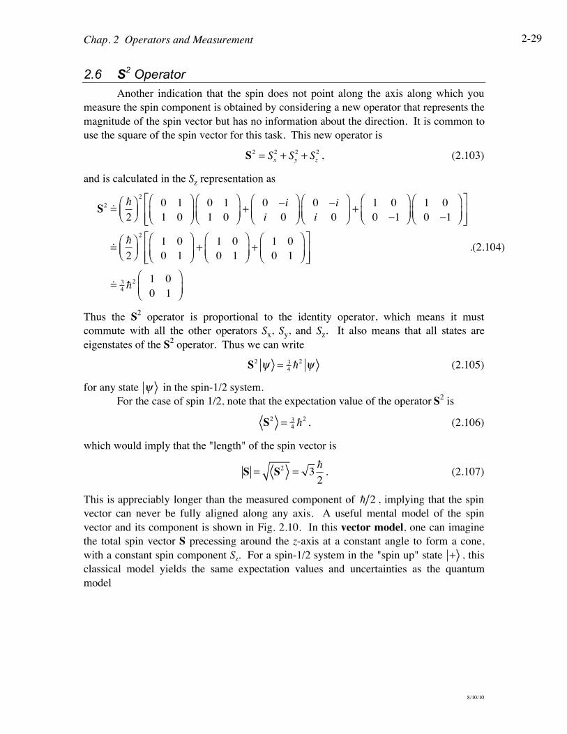
2.6 S2 Operator
Another indication that the spin does not point along the axis along which you
measure the spin component is obtained by considering a new operator that represents the
magnitude of the spin vector but has no information about the direction. It is common to
use the square of the spin vector for this task. This new operator is
S2= Sx
2+ Sy
2+ Sz
2 , (2.103)
and is calculated in the Sz representation as
S2!"
2
!"#
$%&2
0 1
1 0
!
"#$
%&0 1
1 0
!
"#$
%&+
0 'ii 0
!
"#$
%&0 'ii 0
!
"#$
%&+
1 0
0 '1!
"#$
%&1 0
0 '1!
"#$
%&(
)**
+
,--
!"
2
!"#
$%&2
1 0
0 1
!
"#$
%&+
1 0
0 1
!
"#$
%&+
1 0
0 1
!
"#$
%&(
)**
+
,--
!3
4"2 1 0
0 1
!
"#$
%&
.(2.104)
Thus the S2 operator is proportional to the identity operator, which means it must
commute with all the other operators Sx, Sy, and Sz. It also means that all states are
eigenstates of the S2 operator. Thus we can write
S2 ! =
3
4!2 ! (2.105)
for any state ! in the spin-1/2 system.
For the case of spin 1/2, note that the expectation value of the operator S2 is
S2=
3
4!2, (2.106)
which would imply that the "length" of the spin vector is
S = S2
= 3!
2. (2.107)
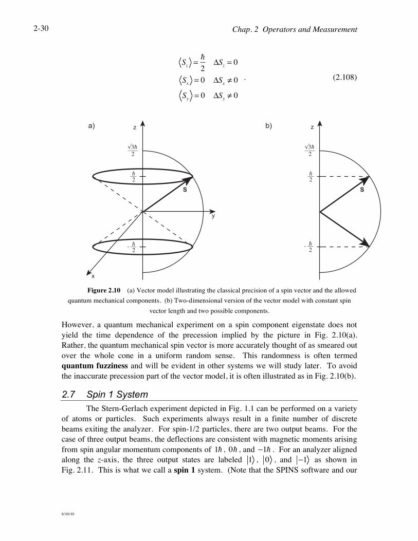
This is appreciably longer than the measured component of ! 2 , implying that the spin
vector can never be fully aligned along any axis. A useful mental model of the spin
vector and its component is shown in Fig. 2.10. In this vector model, one can imagine
the total spin vector S precessing around the z-axis at a constant angle to form a cone,
with a constant spin component Sz. For a spin-1/2 system in the "spin up" state + , this
classical model yields the same expectation values and uncertainties as the quantum
model
Chap. 2 Operators and Measurement
8/10/10
2-30
Sz =!
2!Sz = 0
Sx = 0 !Sx " 0
Sy = 0 !Sy " 0
. (2.108)
S
z
y
x
a)
!2
"3!2
S
b)
!2
"3!2
!2-
!2-
z
Figure 2.10 (a) Vector model illustrating the classical precision of a spin vector and the allowed
quantum mechanical components. (b) Two-dimensional version of the vector model with constant spin
vector length and two possible components.
However, a quantum mechanical experiment on a spin component eigenstate does not
yield the time dependence of the precession implied by the picture in Fig. 2.10(a).
Rather, the quantum mechanical spin vector is more accurately thought of as smeared out
over the whole cone in a uniform random sense. This randomness is often termed
quantum fuzziness and will be evident in other systems we will study later. To avoid
the inaccurate precession part of the vector model, it is often illustrated as in Fig. 2.10(b).
2.7 Spin 1 System
The Stern-Gerlach experiment depicted in Fig. 1.1 can be performed on a variety
of atoms or particles. Such experiments always result in a finite number of discrete
beams exiting the analyzer. For spin-1/2 particles, there are two output beams. For the
case of three output beams, the deflections are consistent with magnetic moments arising
from spin angular momentum components of 1! , 0! , and !1! . For an analyzer aligned
along the z-axis, the three output states are labeled 1 , 0 , and !1 as shown in
Fig. 2.11. This is what we call a spin 1 system. (Note that the SPINS software and our
Chap. 2 Operators and Measurement
8/10/10
2-31
Stern-Gerlach schematics use arrows for the 1 and !1 output beams, but these outputs
are not the same as the spin-1/2 states that are also denoted with arrows.)
The three eigenvalue equations for the spin component operator Sz of a spin-1
system are
Sz1 = ! 1
Sz0 = 0! 0
Sz!1 = !! !1
. (2.109)
As we did in the spin-1/2 case, we choose the Sz basis as the standard basis in which to
express kets and operators using matrix representation. In section 2.1, we found that
eigenvectors are unit vectors in their own basis and an operator is always diagonal in its
own basis. Using the first rule, we can immediately write down the eigenvectors of the Sz
operator:
1 !
1
0
0
!
"
##
$
%
&&
0 !
0
1
0
!
"
##
$
%
&&
'1 !
0
0
1
!
"
##
$
%
&&
(2.110)
where we again use the convention that the ordering of the rows follows the eigenvalues
in descending order. Using the second rule, we write down the Sz operator
Sz!
1" 0 0
0 0" 0
0 0 !1"
"
#
$$
%
&
''= "
1 0 0
0 0 0
0 0 !1
"
#
$$
%
&
''
(2.111)
with the eigenvalues 1! , 0! , and !1! ordered along the diagonal. The value zero is a
perfectly valid eigenvalue in some systems.
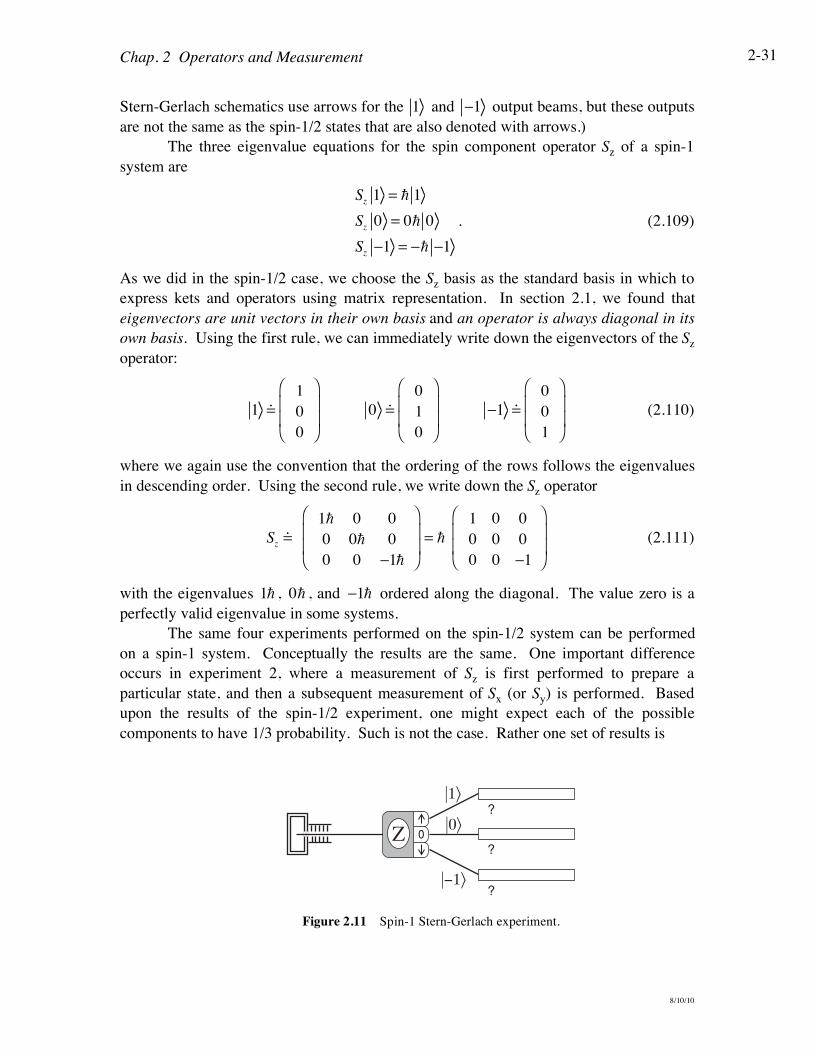
The same four experiments performed on the spin-1/2 system can be performed
on a spin-1 system. Conceptually the results are the same. One important difference
occurs in experiment 2, where a measurement of Sz is first performed to prepare a
particular state, and then a subsequent measurement of Sx (or Sy) is performed. Based
upon the results of the spin-1/2 experiment, one might expect each of the possible
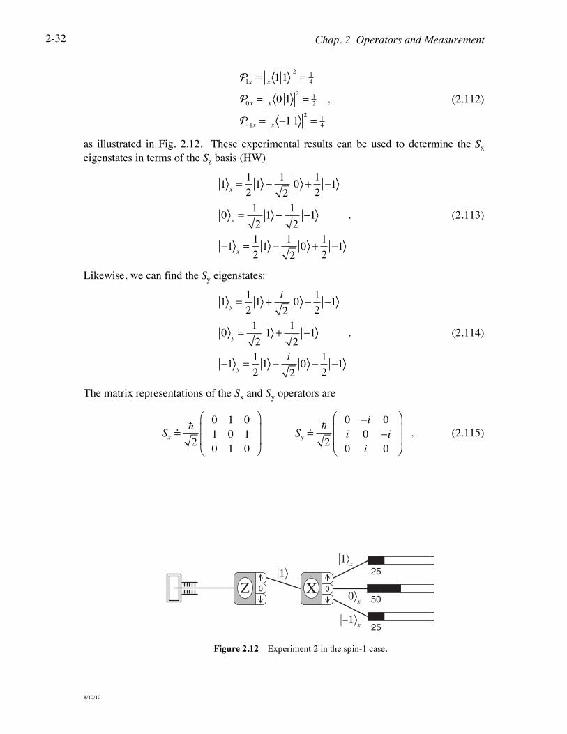
components to have 1/3 probability. Such is not the case. Rather one set of results is
?
?
|1%
|&1%
Z 0 |0%
?
Figure 2.11 Spin-1 Stern-Gerlach experiment.
Chap. 2 Operators and Measurement
8/10/10
2-32
!1x=
x1 1
2
=1
4
!0x=
x0 1
2
=1
2
!!1x
=x!1 1
2
=1
4
, (2.112)
as illustrated in Fig. 2.12. These experimental results can be used to determine the Sx
eigenstates in terms of the Sz basis (HW)
1x=1
21 +
1
20 +
1
2!1
0x=1
21 !
1
2!1
!1x=1
21 !
1
20 +
1
2!1
. (2.113)
Likewise, we can find the Sy eigenstates:
1y=1
21 +
i
20 !
1
2!1
0y=1
21 +
1
2!1
!1y=1
21 !
i
20 !
1
2!1
. (2.114)
The matrix representations of the Sx and Sy operators are
Sx !"
2
0 1 0
1 0 1
0 1 0
!
"
##
$
%
&&
!!!!!!!!Sy !"
2
0 'i 0
i 0 'i0 i 0
!
"
##
$
%
&&
, (2.115)
25
25
|1%x
X 050
|1%
|0%x
|&1%x
Z 0
Figure 2.12 Experiment 2 in the spin-1 case.
Chap. 2 Operators and Measurement
8/10/10
2-33
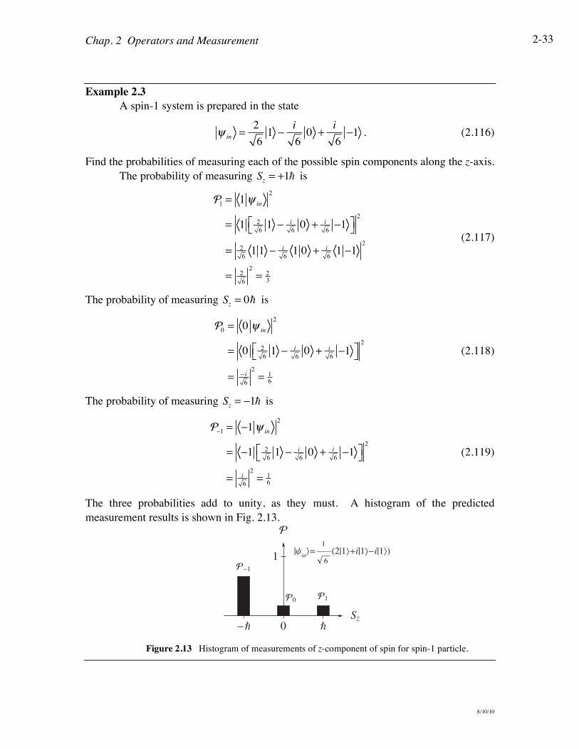
Example 2.3
A spin-1 system is prepared in the state
!in
=2
61 "
i
60 +
i
6"1 . (2.116)
Find the probabilities of measuring each of the possible spin components along the z-axis.
The probability of measuring Sz= +1! is
!1= 1!
in
2
= 12
61 " i
60 +
i
6"1#$ %&
2
=2
61 1 " i
61 0 +
i
61 "1
2
=2
6
2
=2
3
(2.117)
The probability of measuring Sz= 0! is
!0= 0 !
in
2
= 02
61 " i
60 +
i
6"1#$ %&
2
=" i6
2
=1
6
(2.118)
The probability of measuring Sz= !1! is
!!1 = !1"in
2
= !1 2
61 ! i
60 +
i
6!1#$ %&
2
=i
6
2
=1
6
(2.119)
The three probabilities add to unity, as they must. A histogram of the predicted
measurement results is shown in Fig. 2.13.
-— 0 —Sz
1
!
!-1
!0 !1
1
6|yinÚ= (2|1Ú+i|1Ú-i|1Ú)
Figure 2.13 Histogram of measurements of z-component of spin for spin-1 particle.
Chap. 2 Operators and Measurement
8/10/10
2-34
To generalize to other possible spin systems, we need to introduce new labels.
We use the label s to denote the spin of the system, such as spin 1/2, spin 1, spin 3/2. The
number of beams exiting a Stern-Gerlach analyzer is 2s +1 . In each of these cases, a
measurement of a spin component along any axis yields results ranging from a maximum
value of s! to a minimum value of !s! , in unit steps of the value ! . We denote the
possible values of the spin component along the z-axis by the label m, the integer or half-
integer multiplying ! . A quantum state with specific values of s and m is denoted as
sm , yielding the eigenvalue equations
S2sm = s s +1( )!2 sm
Szsm = m! sm
. (2.120)
The label s is referred to as the spin angular momentum quantum number or the spin
quantum number for short. The label m is referred to as the spin component quantum
number or the magnetic quantum number because of its role in magnetic field
experiments like the Stern-Gerlach experiment. The connection between this new sm
notation and the spin-1/2 ± notation is
1
2
1
2= +
1
2,! 1
2= !
. (2.121)
For the spin-1 case, the connection to this new notation is
11 = 1
10 = 0
1,!1 = !1
. (2.122)
We will continue to use the ± notation, but will find the new notation useful later
(Chap. 7).
2.8 General Quantum Systems
Let's extend the important results of this chapter to general quantum mechanical
systems. For a general observable A with quantized measurement results an
, the
eigenvalue equation is
A an= a
nan
(2.123)
In the basis formed by the eigenstates an
, the operator A is represented by a matrix
with the eigenvalues along the diagonal
A !
a1
0 0 "
0 a2
0 "
0 0 a3"
# # # $
!
"
####
$
%
&&&&
, (2.124)
Chap. 2 Operators and Measurement
8/10/10
2-35
whose size depends on the dimensionality of the system. In this same basis, the
eigenstates are represented by the column vectors
a1!
1
0
0
"
!
"
####
$
%
&&&&
,!! a2!
0
1
0
"
!
"
####
$
%
&&&&
,!! a3!
0
0
1
"
!
"
####
$
%
&&&&
,!# , (2.125)
The projection operators corresponding to measurement of the eigenvalues an
are
Pan
= anan
. (2.126)
The completeness of the basis states is expressed by saying that the sum of the projection
operators is the identity operator
Pan
n
! = anan
n
! = 1 . (2.127)
2.9 Summary
In this chapter we have extended the mathematical description of quantum
mechanics by using operators to represent physical observables. The only possible
results of measurements are the eigenvalues of operators. The eigenvectors of the
operator are the basis states corresponding to each possible eigenvalue. We find the
eigenvalues and eigenvectors by diagonalizing the matrix representing the operator,
which allows us to predict the results of measurements. The eigenvalue equations for the
spin-1/2 component operator Sz are
Sz+ =
!
2+
Sz! = !
!
2!
, (2.128)
The matrices representing the spin-1/2 operators are
Sx !"
2
0 1
1 0
!
"#$
%&!!!!!!!!!!!!!!Sy !
"
2
0 'ii 0
!
"#$
%&
Sz !"
2
1 0
0 '1!
"#$
%&!!!!!!!!!!!!S
2!3"
2
4
1 0
0 1
!
"#$
%&
. (2.129)
We characterized quantum mechanical measurements of an observable A by the
expectation value
A = ! A ! = an!an
n
" (2.130)
and the uncertainty
Chap. 2 Operators and Measurement
8/10/10
2-36
!A = A2" A
2
. (2.131)
We made a connection between the commutator A,B[ ] = AB ! BA of two
operators and the ability to measure the two observables. If two operators commute, then
we can measure both observables simultaneously, but if they do not commute, then we
cannot measure simultaneously. We quantified this disturbance that measurement inflicts
on quantum systems through the quantum mechanical uncertainty principle
!A!B "1
2[A,B] . (2.132)
We also introduced the projection postulate, which states how the quantum state
vector is changed after a measurement.
2.10 Problems
2.1 Given the following information:
Sx±
x= ±!
2±
x
Sy ±y= ±!
2±
y
±x=1
2+ ± !"# $% ±
y=1
2+ ± i !"# $%
find the matrix representations of Sx and Sy in the Sz basis.
2.2 From the previous problem we know that the matrix representation of Sx in the Sz
basis is
Sx!"
2
0 1
1 0
!
"#$
%&
Diagonalize this matrix to find the eigenvalues and the eigenvectors of Sx.
2.3 Find the matrix representation of Sz in the Sx basis, for spin 1/2. Diagonalize this
matrix to find the eigenvalues and the eigenvectors in this basis. Show that the
eigenvalue equations for Sz are satisfied in this new representation.
2.4 Show by explicit matrix calculation that the matrix elements of a general operator
A (within a spin-1/2 system) are as shown in Eqn. (2.13).
2.5 Calculate the commutators of the spin-1/2 operators Sx, Sy, and Sz, thus verifying
Eqns. (2.96).
Chap. 2 Operators and Measurement
8/10/10
2-37
2.6 Verify that the spin component operator Sn along the direction n has the matrix
representation shown in Eqn. (2.41).
2.7 Diagonalize the spin component operator Sn along the direction n to find its
eigenvalues and the eigenvectors.
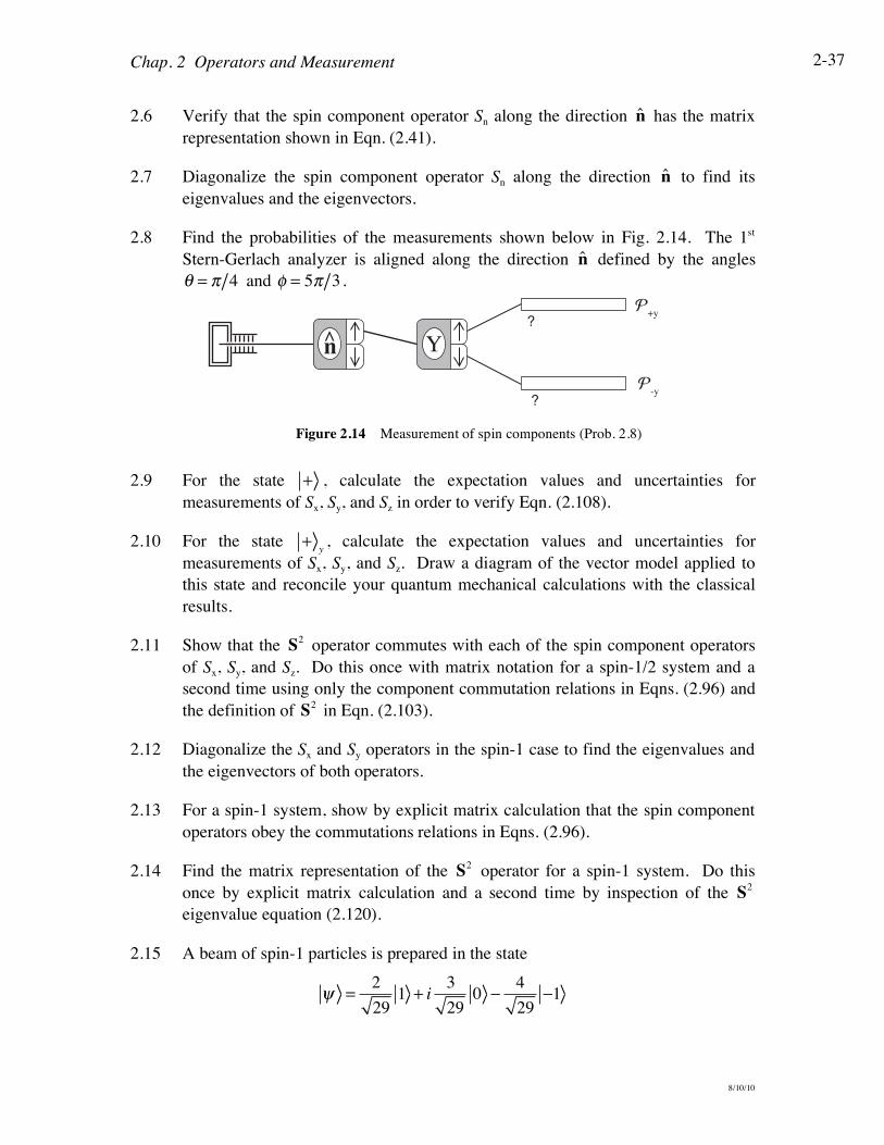
2.8 Find the probabilities of the measurements shown below in Fig. 2.14. The 1st
Stern-Gerlach analyzer is aligned along the direction n defined by the angles
! = " 4 and ! = 5" 3 .
Y?
?
!+y
!-y
n
Figure 2.14 Measurement of spin components (Prob. 2.8)
2.9 For the state + , calculate the expectation values and uncertainties for
measurements of Sx, Sy, and Sz in order to verify Eqn. (2.108).
2.10 For the state +y, calculate the expectation values and uncertainties for
measurements of Sx, Sy, and Sz. Draw a diagram of the vector model applied to
this state and reconcile your quantum mechanical calculations with the classical
results.
2.11 Show that the S2 operator commutes with each of the spin component operators
of Sx, Sy, and Sz. Do this once with matrix notation for a spin-1/2 system and a
second time using only the component commutation relations in Eqns. (2.96) and
the definition of S2 in Eqn. (2.103).
2.12 Diagonalize the Sx and Sy operators in the spin-1 case to find the eigenvalues and
the eigenvectors of both operators.
2.13 For a spin-1 system, show by explicit matrix calculation that the spin component
operators obey the commutations relations in Eqns. (2.96).
2.14 Find the matrix representation of the S2 operator for a spin-1 system. Do this
once by explicit matrix calculation and a second time by inspection of the S2
eigenvalue equation (2.120).
2.15 A beam of spin-1 particles is prepared in the state
! =2
291 + i
3
290 "
4
29"1
Chap. 2 Operators and Measurement
8/10/10
2-38
a) What are the possible results of a measurement of the spin component Sz, and
with what probabilities would they occur?
b) What are the possible results of a measurement of the spin component Sx, and
with what probabilities would they occur?
c) Plot histograms of the predicted measurement results from parts (a) and (b),
and calculate the expectation values for both measurements.
2.16 A beam of spin-1 particles is prepared in the state
! =2
291
y+ i
3
290
y"
4
29"1
y
a) What are the possible results of a measurement of the spin component Sz, and
with what probabilities would they occur?
b) What are the possible results of a measurement of the spin component Sy, and
with what probabilities would they occur?
c) Plot histograms of the predicted measurement results from parts (a) and (b) ,
and calculate the expectation values for both measurements.
2.17 A spin-1 particle is in the state
! !1
30
1
2
5i
"
#
$$
%
&
''
a) What are the possible results of a measurement of the spin component Sz, and
with what probabilities would they occur? Calculate the expectation value of
the spin component Sz.
b) Calculate the expectation value of the spin component Sx. Suggestion: Use
matrix mechanics to evaluate the expectation value.
2.18 A spin-1 particle is prepared in the state
! =1
141 "
3
140 + i
2
14"1
a) What are the possible results of a measurement of the spin component Sz, and
with what probabilities would they occur?
b) Suppose that the Sz measurement on the particle yields the result Sz= !! .
Subsequent to that result a second measurement is performed to measure the
spin component Sx. What are the possible results of that measurement, and
with what probabilities would they occur?
Chap. 2 Operators and Measurement
8/10/10
2-39
c) Draw a schematic diagram depicting the successive measurements in parts (a)
and (b).
2.19 A spin-1 particle is prepared in the state
!i=
1
61 "
2
60 + i
3
6"1 .
Find the probability that the system is measured to be in the final state
! f =1+ i
71
y+2
70
y" i
1
7"1
y.
2.20 In part (2) of SPINS Lab #3, you measured the spin components of the unknown
(spin 1) initial states !i
(i = 1, 2, 3, 4) onto the nine spin eigenstates along the
three axes. Using your measured values, deduce the unknown initial states.
2.21 In part (3) of SPINS Lab #3, you built a spin-1 interferometer and measured the
relative probabilities after the final Stern-Gerlach analyzer for the seven possible
cases where one beam, a pair of beams, or all three beams from the 2nd Stern-
Gerlach analyzer were used. Show how you used the projection postulate to
calculate the theoretical probabilities.
2.22 A beam of spin-1/2 particles is sent through a series of three Stern-Gerlach
analyzers, as shown in Fig. 2.15. The 2nd Stern-Gerlach analyzer is aligned along
the n direction, which makes an angle ! in the x-z plane with respect to the z-axis.
Z?
?
nZ
Figure 2.15 Measurement of spin components (Prob. 2.22)
a) What fraction of the particles transmitted through the 1st Stern-Gerlach
analyzer are measured to have spin down at the 3rd Stern-Gerlach analyzer?
b) How must the angle ! of the 2nd Stern-Gerlach analyzer be oriented so as to
maximize the number of particles measured to have spin down at the 3rd Stern-
Gerlach analyzer? What is this maximum fraction?
c) What fraction of the particles have spin down at the 3rd Stern-Gerlach analyzer
if the 2nd Stern-Gerlach analyzer is removed from the experiment?
2.23 Consider a three dimensional ket space. In the basis defined by three orthogonal
kets 1 , 2 , and 3 , the operators A and B are represented by
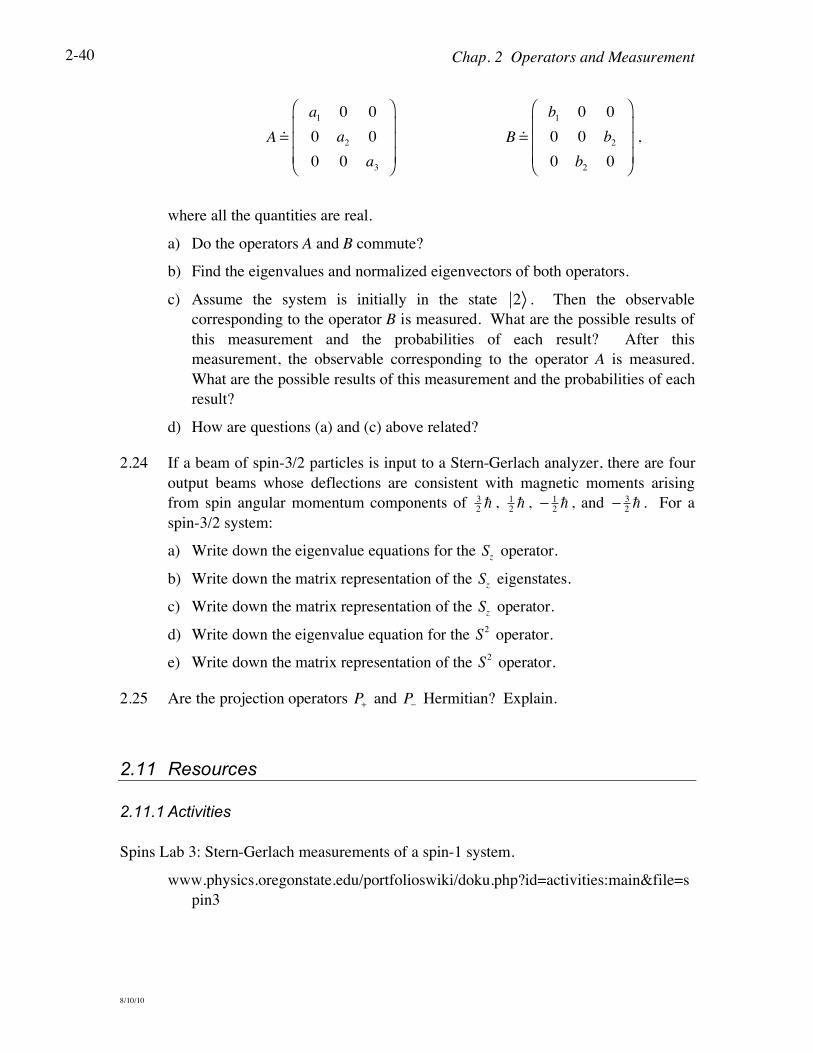
Chap. 2 Operators and Measurement
8/10/10
2-40
A !
a1
0 0
0 a2
0
0 0 a3
!
"
###
$
%
&&&
B !
b1
0 0
0 0 b2
0 b2
0
!
"
###
$
%
&&&
,
where all the quantities are real.
a) Do the operators A and B commute?
b) Find the eigenvalues and normalized eigenvectors of both operators.
c) Assume the system is initially in the state 2 . Then the observable
corresponding to the operator B is measured. What are the possible results of
this measurement and the probabilities of each result? After this
measurement, the observable corresponding to the operator A is measured.
What are the possible results of this measurement and the probabilities of each
result?
d) How are questions (a) and (c) above related?
2.24 If a beam of spin-3/2 particles is input to a Stern-Gerlach analyzer, there are four
output beams whose deflections are consistent with magnetic moments arising
from spin angular momentum components of
3
2! ,
1
2! ,
!1
2! , and
!3
2! . For a
spin-3/2 system:
a) Write down the eigenvalue equations for the Sz operator.
b) Write down the matrix representation of the Sz eigenstates.
c) Write down the matrix representation of the Sz operator.
d) Write down the eigenvalue equation for the S2 operator.
e) Write down the matrix representation of the S2 operator.
2.25 Are the projection operators P+
and P!
Hermitian? Explain.
2.11 Resources
2.11.1 Activities
Spins Lab 3: Stern-Gerlach measurements of a spin-1 system.
www.physics.oregonstate.edu/portfolioswiki/doku.php?id=activities:main&file=s
pin3

Chap. 2 Operators and Measurement
8/10/10
2-41
2.11.2 Further reading