FY1003 ELEKTRISITET OG MAGNETISME

Project paper on:

Radio Astronomy

- Radio Telescopes -

Kristin BorckAndrea Klubicka

23/04-2004

1

Abstract

We introduce the most general types of radio telescopes and describe how theseoperate; starting from the simplest type, the single aperture telescope, then moving on to thefunction of a radio telescope consisting of two apertures and finally presenting the mostcomplex combinations. The theory behind electromagnetic waves and how they radiate, isoccupying a rather big part of this paper, as it is essential in understanding how radiotelescopes function. Examples and a description of the origins of radio waves from space arealso presented, and a detailed explanation of radio signals and noise is included to bring evenmore clarity on the subject of radio telescopes.

Introduction [1-3]

Almost everything we know about the universe, about stars and stellar systems, theirdistribution, kinematics and dynamics, has been obtained from information brought to us byelectromagnetic radiation. Only a small part of our knowledge stems form material sources ofinformation, such as meteorites that hit the surface of the Earth, cosmic particles of radiationor samples of material collected by manned or unmanned space probes.

For thousands of years, all the information that astronomers gathered about theuniverse was based on visible light. In the twentieth century, however, the wavelength rangewas slightly expanded. Radio waves were the first part of the electromagnetic spectrumbeyond the visible light to be exploited for astronomy. Karl Jansky, a young electrical engineerat Bell Telephone Laboratories, was the first to discover these waves. This happened in theearly 1930s, as he was trying to locate what was causing interference with the then-newtransatlantic radio link at a wavelength of 14.6 m. He realized that one kind of radio noise isstrongest when the constellation Sagittarius is high in the sky. Since the center of our galaxy islocated in the direction of Sagittarius, he concluded that he was detecting radio waves from asource beyond the Earth. As Jansky continued his observations, he showed that the principalsources of radiation were distributed throughout the Milky Way, and that the radiation couldnot be from stellar sources similar to the Sun.

Jansky’s observations were taken up and improved by the radio engineer Grote Reber.In 1936 he built the first radio telescope, a radio-wave detector dedicated to astronomy. In theyears from 1938 to 1944 Reber did his measurements at wavelengths of 1.9 m and 0.63 m. Hedetected radio waves emitted from the entire Milky Way, with the greatest emission from thecenter of the galaxy. These observations were published in the Astrophysical Journal in 1944.

Radio physics made great progress during World War II, mainly due to thedevelopment of sensitive and efficient radar equipment. After the end of the war, newreceivers were instrumental in opening up the new radio window in the Earth’s atmosphere.The radio window reaching from λ ≅ 10-15 m to about λ ≅ 0.1 mm or less was the first newspectral range that became available to astronomy outside the slightly expanded opticalwindow. Soon different new objects could be discovered, and the new astronomical discipline

2

of radio astronomy contributed to changing our views on many subjects, requiring mechanismsfor their explanation that differed considerably from those commonly used in “optical”astrophysics.

In the years since 1945 technological progress permitted the opening up of severaladditional spectral windows of widely different wavelength ranges, such as infrared,ultraviolet and X-ray. Each spectral window requires its own technology, and the ways ofdoing measurements differ for each. Therefore astronomers view these different techniques asdifferent sections of astronomy: radio astronomy, infrared astronomy, X-ray astronomy and soon.

This paper concentrates mostly on the principals behind the simplest type of radiotelescope, explaining the concepts of angular resolution, sensitivity and such. An application toa two element telescope is also presented, and finally we mention the generalization to Nelement telescopes.

Electromagnetic Radiation [1, 4]

Maxwell’s equations are today the foundation of most physical phenomena around us,and every physical law in electromagnetism can be deduced from these four equations. Theyare distinct because they effectively describe both static and time dependent fields.

Maxwell’s equations in free space:

0E∇ ⋅ =r

(1)

0B∇ ⋅ =r

(2)

BE

t∂

∇× = −∂

rr

(3)

0 0

EB

tµ ε

∂∇× =

∂

rr

(4)

The theory of EM waves and the associated laws and properties are a naturalconsequence of these equations. When not considering propagation through empty space,Gauss law for electric fields (1),states that the total electric flux through a closed surfaceequals the net charge inside that surface (divided by ε0). This law relates the electric field tothe charge distribution, where electric field lines originate from positive charges and end up onnegative charges. Gauss’ law for magnetism, (2), shows that the net magnetic flux through aclosed surface is zero, meaning that the number of field lines entering a surface, equals thenumber leaving it. This proves that magnetic field lines cannot begin or end at any point.Maxwell-Ampères law,(4), predicts how a time dependent electric field will produce amagnetic field, while Faraday’s law,(3) indicates the opposite. By applying the curl andcombining these two latter equations, the wave equation is obtained both for the electric andmagnetic field, respectively:

3

22

0 0 2( ) ( ) ( ) ( )B B E

E E E Bt t t

µ ε∂ ∂ ∂

∇× ∇× = ∇ ∇ ⋅ − ∇ = ∇ × − = − ∇× = −∂ ∂ ∂

r r rr r r r

, (5)

22

0 0 0 0 0 0 2( ) ( ) ( ) ( )E B

B B B Et t t

µ ε µ ε µ ε∂ ∂ ∂

∇× ∇× = ∇ ∇ ⋅ − ∇ = ∇ × = ∇× = −∂ ∂ ∂

r rr r r r

, (6)

and since 0E∇ ⋅ =r

and 0B∇ ⋅ =r

,

2 22 2

0 0 0 02 2 and E B

E Bt t

µ ε µ ε∂ ∂

∇ = ∇ =∂ ∂

r rr r

(7a) and (7b)

Still considering propagation through empty space, where Q = 0 and I = 0, Maxwell’sequations provide an important result, namely that the wave velocity is equal to c, the speed oflight. We can also deduce the fact that at every instant, the ratio of the electric field to themagnetic field of an electromagnetic wave equals this same constant.

From electrostatics we know that stationary electric charges generate electric fields,while accelerating charges generate propagating electric and magnetic fields, i.e. EM waves.These fields are positioned at right angles to each other and to the direction of the wavepropagation. Thus, EM waves are transverse. When an electromagnetic wave leaves its source,it spreads out in straight lines and its oscillating fields weaken with distance, according to therelation 1/r. Thus, the concentration of electromagnetic waves gets smaller as the distance fromthe source gets bigger. This accounts for the loss of signal strength by the time radiation fromouter space reaches us.

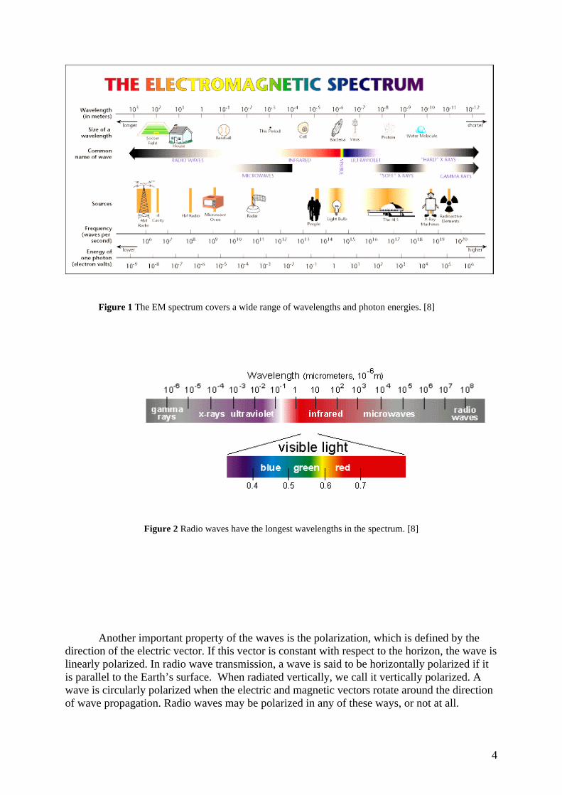
Which type of electromagnetic wave we are dealing with is determined by thefrequency of the wave. For higher frequencies than our eyes can detect, we have ultravioletradiation, x-rays and gamma rays. On the other side of the spectrum there is infrared radiationand radio waves. Associated with the frequency is the concept of wavelength. Since all theelectromagnetic waves travel through vacuum with the speed of light, their frequency f andwavelength λ are related by the equation f λ = c. There is really no upper limit to the value ofthe radiation frequency. Traveling through different media, different wavelengths do notbehave in the same way. This is why looking at a star with our eyes and through a telescopewill give different images.

.

4

Figure 1 The EM spectrum covers a wide range of wavelengths and photon energies. [8]

Figure 2 Radio waves have the longest wavelengths in the spectrum. [8]

Another important property of the waves is the polarization, which is defined by thedirection of the electric vector. If this vector is constant with respect to the horizon, the wave islinearly polarized. In radio wave transmission, a wave is said to be horizontally polarized if itis parallel to the Earth’s surface. When radiated vertically, we call it vertically polarized. Awave is circularly polarized when the electric and magnetic vectors rotate around the directionof wave propagation. Radio waves may be polarized in any of these ways, or not at all.

5

Electromagnetic waves carry both energy and momentum, so they can exert forces onsurfaces they reach. The rate of flow of energy by an electromagnetic wave is described by the

Poynting vector, Sr

with direction along the wave propagation; 0

1( )S E B

µ= ×

r r r. The average of

Sr

taken over one or more cycles, gives the intensity I of the wave; 20 0

12

I S c Eε= =r

. In

perfect blackbodies, all the radiation impinged will be absorbed, thus the total momentumdelivered by the wave will be /p U c=

r and the radiation pressure will be given by /P S c=

r.

Similarly, perfect reflectors will deliver a momentum value of 2 /p U c=r

, which corresponds

to a radiation pressure of 2 /P S c=r

.

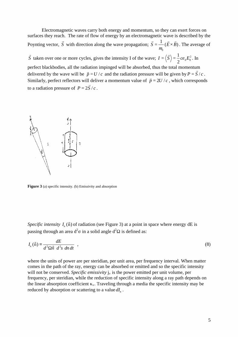
Figure 3 (a) specific intensity. (b) Emissivity and absorption

Specific intensity ˆ(n)Iν of radiation (see Figure 3) at a point in space where energy dE ispassing through an area d2σ in a solid angle d2Ω is defined as:

2 2ˆ(n)

ˆdE

Id n d d dtν σ ν

≡Ω ⋅

, (8)

where the units of power are per steridian, per unit area, per frequency interval. When mattercomes in the path of the ray, energy can be absorbed or emitted and so the specific intensitywill not be conserved. Specific emissivity jν is the power emitted per unit volume, perfrequency, per steridian, while the reduction of specific intensity along a ray path depends onthe linear absorption coefficient κν. Traveling through a media the specific intensity may bereduced by absorption or scattering to a value dIν .

6

The absorption coefficient is defined by

dI I dsν ν νκ= − , (9)

provided that the system is in a steady-state equilibrium. How specific intensity behaves alonga ray path is described by the equation of radiative matter:

dIj I

dsν

ν ν νκ= − , (10)

From this equation, some solutions can be given immediately, like Kirchhoff’s law:

( )j

B Tνν

νκ= , (11)

where ( )B Tν is Planck’s function (34). Other simple solutions are obtained for emission and

absorption only. A ray with specific intensity 0fI at the origin has,

0

0( ) ( ') ' (emission only)

S

f f fI s I j s ds= + ∫ (12)

0( ') ' 0( ) (absorption only)

S

f s ds

f fI s I eκ−∫= (13)

Electromagnetic waves can traverse the same space independently of one another andthey have the property of superposition and interference. Another way of describing EMradiation is by photons. These can be thought of as small packets of energy with no mass thattravel at the speed of light. When considered this way, the waves are characterized by theenergy of each photon.

7

Thermal processes

As mentioned above, by regular changes in the electric and magnetic fields,electromagnetic waves are generated and they transport energy from point to point. This can beeither a thermal or a non-thermal process. For energy to be transported thermally, it is requiredthat the body emitting the radiation has thermal energy (temperature). This includes all bodieswith a temperature above the absolute zero. Common examples of thermal radiation areblackbody radiation, free-free emission ("bremsstrahlung") in an ionized gas and spectral lineemission. A blackbody is a hypothetical object that absorbs one hundred percent of the energythat reaches it, and reflects nothing. When it reaches an equilibrium temperature, it startsradiating energy. The characteristic wavelength of this radiation is maintained by thetemperature. Free-free emission comes from ionized gas. Ionization happens when electronsare removed from atoms. When charged particles later move around in this plasma, they causeacceleration of electrons and hence the gas cloud emits radiation. Spectral line emissioninvolves the transition of electrons in atoms from a high energy level to a lower energy level.When this happens, a photon is emitted with the same energy as the energy difference betweenthe two levels. The emission of this photon at a certain discrete energy shows up as a discrete"line" or wavelength in the electromagnetic spectrum.

Non-thermal processes

In conclusion, all objects that radiate thermally will send out end receive energy of allfrequencies. Some will emit mostly at ultraviolet frequencies, while others will mostly emit atinfrared and the decisive factor is the temperature. Not many thermal stellar objects can beobserved by the radio waves they release, but the ones that do are the Sun and some starscovered by stellar winds. Radio frequencies are best discovered from objects that emit non-thermal radiation. This mechanism is related to the interaction of charged particles withmagnetic fields. A charged particle entering a magnetic field will begin moving in a circularor spiral path, an since it then accelerates it will give off energy. When the speed of thisparticle is comparable to the speed of light, it will emit synchrotron radiation. Most commonly,these particles are electrons. The frequency of the radiation is directly related to how fast theparticle is traveling. The longer the particle stays in the magnetic field, the more energy itloses. As a result, the particle makes a wider spiral around the magnetic field, and emitselectromagnetic radiation at a longer wavelength. To maintain synchrotron radiation, acontinuous supply of relativistic particles is necessary. Typically, these are supplied by verypowerful energy sources such as supernova remnants, quasars, or other forms of active galacticnuclei.

Masers (micro-wave-amplified stimulated emission of radiation) display another typeof non-thermal radiation. They can be compared to lasers (which amplify radiation at or nearvisible wavelengths). This interstellar medium contains a small number of certain molecules,which would normally be very hard to detect, but due to “masing”, these clouds can even bedetected in different galaxies, because maser action will amplify faint emission lines at aspecific frequency.

8

A third type of non-thermal radiation is gyrosynchrotron emission from pulsars. Thisprocess is actually just a special form of synchrotron emission. Pulsars are the result of thedeath of massive stars. As a massive star runs out of “fuel”, its core begins to collapse, theouter layers of the star fall down onto the core and a shock wave is produced that results in asupernova explosion. After the explosion, an extremely dense neutron star is left behind. Arapidly rotating neutron star is known as a pulsar. A typical pulsar has a magnetic field atrillion times stronger than the Earth's, which accelerates particles to nearly the speed of light,causing them to emit radiation, including radio waves. When this radiation reaches Earth, wesee a "pulse" of radiation from the pulsar.

Radio Waves [1,6]

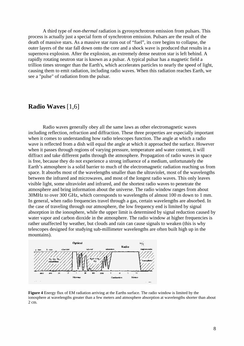
Radio waves generally obey all the same laws as other electromagnetic wavesincluding reflection, refraction and diffraction. These three properties are especially importantwhen it comes to understanding how radio telescopes function. The angle at which a radiowave is reflected from a dish will equal the angle at which it approached the surface. Howeverwhen it passes through regions of varying pressure, temperature and water content, it willdiffract and take different paths through the atmosphere. Propagation of radio waves in spaceis free, because they do not experience a strong influence of a medium, unfortunately theEarth’s atmosphere is a solid barrier to much of the electromagnetic radiation reaching us fromspace. It absorbs most of the wavelengths smaller than the ultraviolet, most of the wavelengthsbetween the infrared and microwaves, and most of the longest radio waves. This only leavesvisible light, some ultraviolet and infrared, and the shortest radio waves to penetrate theatmosphere and bring information about the universe. The radio window ranges from about30MHz to over 300 GHz, which corresponds to wavelengths of almost 100 m down to 1 mm.In general, when radio frequencies travel through a gas, certain wavelengths are absorbed. Inthe case of traveling through our atmosphere, the low frequency end is limited by signalabsorption in the ionosphere, while the upper limit is determined by signal reduction caused bywater vapor and carbon dioxide in the atmosphere. The radio window at higher frequencies israther unaffected by weather, but clouds and rain can cause signals to weaken (this is whytelescopes designed for studying sub-millimeter wavelengths are often built high up in themountains).

Figure 4 Energy flux of EM radiation arriving at the Earths surface. The radio window is limited by theionosphere at wavelengths greater than a few meters and atmosphere absorption at wavelengths shorter than about2 cm.

9

The refractive index for water vapor is almost twenty times greater at radio than opticalwavelengths. This is due to the permanent dipole moment of water molecules. Refractivity Nof the atmosphere at radio wavelengths and temperatures encountered in the atmosphere isgiven by:

1 177.6 ( 4810 )d vN T P PT− −= + (14)

This is called the Smith and Weitraub formula, where dP denotes the partial pressure of dry airand vP the partial pressure of water vapour (both in millibars). When refraction of radio wavesoccurs in the atmosphere, the arrival of the wavefront at a radio telescope is affected in muchthe same way as for an optical telescope. The apparent increase z∆ in elevation at zenith anglez is

( 1) tanz n z∆ = − , (15)

n being the refractive index of air at radio wavelengths.

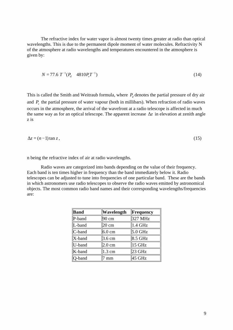
Radio waves are categorized into bands depending on the value of their frequency.Each band is ten times higher in frequency than the band immediately below it. Radiotelescopes can be adjusted to tune into frequencies of one particular band. These are the bandsin which astronomers use radio telescopes to observe the radio waves emitted by astronomicalobjects. The most common radio band names and their corresponding wavelengths/frequenciesare:

Band Wavelength FrequencyP-band 90 cm 327 MHzL-band 20 cm 1.4 GHzC-band 6.0 cm 5.0 GHzX-band 3.6 cm 8.5 GHzU-band 2.0 cm 15 GHzK-band 1.3 cm 23 GHzQ-band 7 mm 45 GHz

10

Signal detection and noise [1-2]

According to the laws of quantum mechanics and the second law of thermodynamicsthe accuracy of all observations will be limited by the fundamental fluctuations that aregenerally known as noise. For the radio astronomer, the detected signal is the sum of both thecosmic signal and the noise generated by the environment, both with a Gaussian character. Aradiometer is used to distinguish the astronomical signal from the interfering noise. Thesignal-to-noise ratio is limited by a system noise consisting of sky background noise andreceiver noise, and it depends on the duration τ of the observation and the bandwidth B of thedetecting system. The estimate of the system noise gets better as the averaging time increases,but an uncertainty always remains. In this part we deal with the waveform and spectrum ofnoise, and we mention some principles of radiometers, which measure the noise power.

Gaussian noiseThe detected signal is a superposition of an infinite assemblage of oscillators with

random frequency and phase. The signal amplitude V(t) is a stationary random variable, andthe properties of the signal can only be described statistically. Gaussian random noise, forwhich the probability density function is a Gaussian function, is the most common form metwith in practice. At each instant of time, the probability that the signal has an amplitude V isgiven by

( ) 2 2/ 212

Vp V e σ

σ π−= (16)

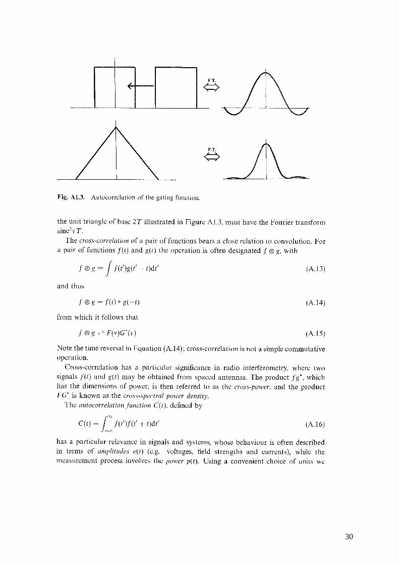
where σ is the standard deviation of the probability density. The mean value of the signalamplitude is zero, and the noise power is the mean value of V(t)2 which, for the givenprobability density, is σ. Another interesting quantity is the autocorrelation function R(τ) of thesignal amplitude, which is defined as

( ) ( ) ( )/ 2

/ 2

T

TT

R V t V t dtτ τ−

= +∫ (17)

where the subscript T indicates that the integration extends over an interval T.

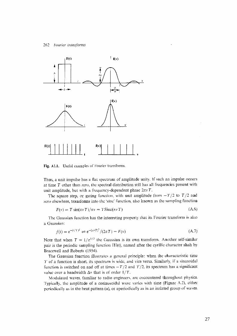
The power spectrum of a random noise signal is the Fourier transform of the autocorrelationfunction. This also has a Gaussian character. In the real world, only an estimate of the signalpower, or its autocorrelation function can be obtained by evaluation over a finite timespan T,so one arrives at an estimate of the power spectrum. This estimate becomes more precise as Tincreases. For a given time interval T the estimated power spectrum is the Fourier transform ofRT(τ):

11

( ) ( )/ 2

/ 2

Ti

T TT

S R e dωτν τ τ−

−

= ∫ (18)

which, in the limit of T going to infinity, becomes

( ) ( ) iS R e dωτν τ τ∞

−

−∞

= ∫ (19)

The spectrum of Gaussian noise is evaluated easily by inspecting equation (3) for the cases ofzero and non-zero time lag. When τ is non-zero, the integral goes to zero since V(t) iscompletely uncorrelated from one instant to the next. When τ = 0, however, the integral tendstowards the mean square deviation, ⟨σ2⟩. For a sufficiently long integration time, therefore, theautocorrelation function is a δ-function for a Gaussian random signal:

( ) ( )2limT

R tτ σ δ→∞

= (20)

The Fourier transform of the δ-function is constant (unity), from which it follows thatGaussian noise has a flat power spectrum with a power spectral density which equals σ2. Theflat power spectrum contains all frequencies and is therefore often called a white spectrum,from the colour analogy.

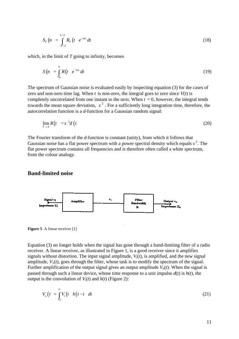
Band-limited noise

Figure 5 A linear receiver [1]

Equation (3) no longer holds when the signal has gone through a band-limiting filter of a radioreceiver. A linear receiver, as illustrated in Figure 1, is a good receiver since it amplifiessignals without distortion. The input signal amplitude, Vi(t), is amplified, and the new signalamplitude, V1(t), goes through the filter, whose task is to modify the spectrum of the signal.Further amplification of the output signal gives an output amplitude Vo(t). When the signal ispassed through such a linear device, whose time response to a unit impulse δ(t) is h(t), theoutput is the convolution of Vi(t) and h(t) (Figure 2):

( ) ( ) ( )o iV t V h t dτ τ τ∞

−∞

= −∫ (21)

12

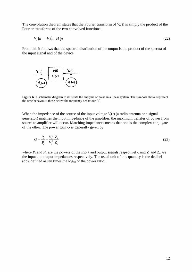
The convolution theorem states that the Fourier transform of Vo(t) is simply the product of theFourier transforms of the two convolved functions:

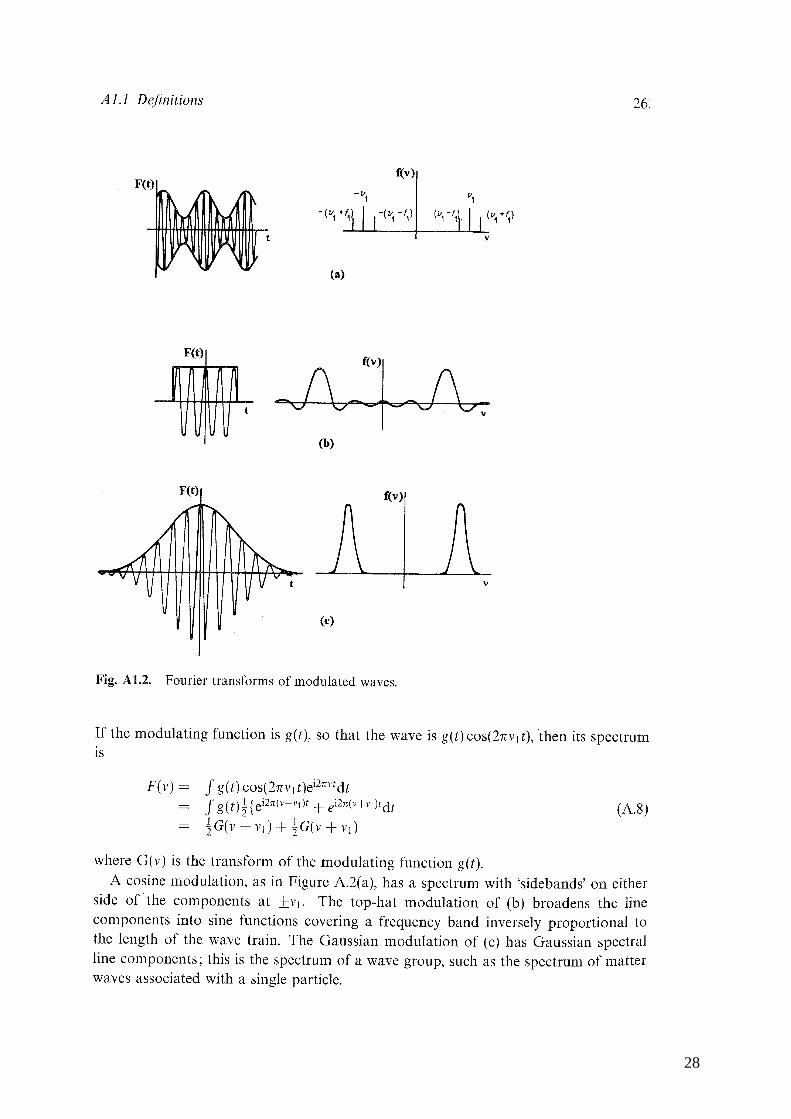
( ) ( ) ( )o iV V Hν ν ν= (22)

From this it follows that the spectral distribution of the output is the product of the spectra ofthe input signal and of the device.

Figure 6 A schematic diagram to illustrate the analysis of noise in a linear system. The symbols above representthe time behaviour, those below the frequency behaviour [2]

When the impedance of the source of the input voltage Vi(t) (a radio antenna or a signalgenerator) matches the input impedance of the amplifier, the maximum transfer of power fromsource to amplifier will occur. Matching impedances means that one is the complex conjugateof the other. The power gain G is generally given by

2

2o o i

i i o

P V ZG

P V Z= = (23)

where Pi and Po are the powers of the input and output signals respectively, and Zi and Zo arethe input and output impedances respectively. The usual unit of this quantity is the decibel(db), defined as ten times the log10 of the power ratio.

13

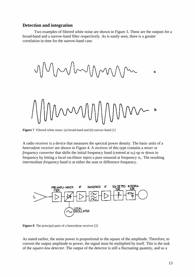
Detection and integrationTwo examples of filtered white noise are shown in Figure 3. These are the outputs for a

broad-band and a narrow-band filter respectively. As is easily seen, there is a greatercorrelation in time for the narrow-band case.

Figure 7 Filtered white noise: (a) broad-band and (b) narrow-band [1]

A radio receiver is a device that measures the spectral power density. The basic units of aheterodyne receiver are shown in Figure 4. A receiver of this type contains a mixer orfrequency converter that shifts the initial frequency band (centred at ν0) up or down infrequency by letting a local oscillator inject a pure sinusoid at frequency ν1. The resultingintermediate frequency band is at either the sum or difference frequency.

Figure 8 The principal parts of a heterodyne receiver [2]

As stated earlier, the noise power is proportional to the square of the amplitude. Therefore, toconvert the output amplitude to power, the signal must be multiplied by itself. This is the taskof the square-law detector. The output of the detector is still a fluctuating quantity, and so a

14

time average of the power is taken, usually by an integrator. Integration of the signal powerfor a time τ gives the average power readout ⟨P⟩, which is an estimate of the signal poweracross the band:

( ) ( )/ 2 / 2

2

/ 2 / 2

T T

d oT T

P p t dt V t dt− −

= = ∫ ∫ (24)

where pd(t) is the instantaneous power measured by the detector and equals the square of theoutput amplitude Vo(t). The resulting power spectrum observed at the detector output is1

( ) ( ) ( ) ( ) ( )2 0 2 ' ' 'd o o oS R S H dν δ ν ν ν ν ν∞

−∞

= + −∫ (25)

The first term on the right-hand side would give the average power for a white noise signal,and the second term, the convolution, expresses the fact that the white noise signal has gonethrough a filter that induces correlation in the output signal.

There is an uncertainty in this final measurement. Since the power density is almost alwaysmeasured with respect to the equivalent temperature Teq of an input load, Teq is a natural unit ofpower density. In the pre-detection (post-filtered signal) there is a correlation for a time ofabout 1/B, from which it follows that there are about B independent measurements per unittime. If the detected signal is integrated for a time τ, there will be a total of about Bτindependent measurements of the filtered noise signal. Since the input noise is random, therelative uncertainty, ∆T, in the measurement of the noise temperature, Ts, at the input of thedetector, will be

sTT

Bτ∆ = (26)

1 A detailed treatment of the squaring process, and the resulting character of the detected signal can be found in[2].

15

Radio Telescopes [1, 4-6]

Radio telescopes are used to study radio emissions from stars, galaxies, quasars, andother astronomical objects. The results of these studies are presented as measurements ofintensity and state of polarization as functions of frequency, angular position and time. Mosttelescopes are able to observe emissions at frequencies ranging from about 30MHz to 300GHzand they work best with wavelengths between 1 and 20cm. Since small structures can be builtwith greater precision than larger ones, radio telescopes designed for operation at millimeterwavelength are typically only a few tens of meters across, whereas those designed foroperation at centimeter wavelengths range up to 100 meters in diameter.

The typical radio telescope consists of a radio receiver and an antenna system. Theantenna or aperture collects radiation which is then transformed to an electric signal by areceiver, called the radiometer. This signal is then amplified, detected and integrated, and theoutput is registered on a recording device.

Radio telescopes are used as single operating apparatuses, in combinations of two, orarrangements of many can be used to study just one phenomenon. Some telescopes are alsodesigned for studying milimetre and sub-milimeter wavelengths. Usually, the typical radiotelescope will measure broad bandwidth continuum radiation, but also the study ofspectroscopic features is common. Modern types observe simultaneously at a large number offrequencies by dividing the signals up into several thousand separate frequency channels thatmay range over a total bandwidth of tens to hundreds of megahertz.

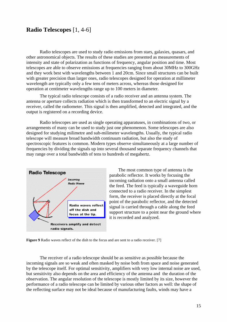
The most common type of antenna is theparabolic reflector. It works by focusing theincoming radiation onto a small antenna calledthe feed. The feed is typically a waveguide hornconnected to a radio receiver. In the simplestform, the receiver is placed directly at the focalpoint of the parabolic reflector, and the detectedsignal is carried through a cable along the feedsupport structure to a point near the ground whereit is recorded and analyzed.

Figure 9 Radio waves reflect of the dish to the focus and are sent to a radio receiver. [7]

The receiver of a radio telescope should be as sensitive as possible because theincoming signals are so weak and often masked by noise both from space and noise generatedby the telescope itself. For optimal sensitivity, amplifiers with very low internal noise are used,but sensitivity also depends on the area and efficiency of the antenna and the duration of theobservation. The angular resolution of the telescope is mostly limited by its size, however theperformance of a radio telescope can be limited by various other factors as well: the shape ofthe reflecting surface may not be ideal because of manufacturing faults, winds may have a

16

powerful effect, there may be thermal deformations (expansion and contraction) anddeflections due to changes in gravitational forces as the antenna is pointed to different parts ofthe sky. The largest effects are gravitational deformations, but these can be minimized bystructural design, for example by allowing the reflector to deform. For instance, if theelevation of the telescope changes, the feed system can be moved to compensate for anychange in axis and focal length.

Single aperture telescopes

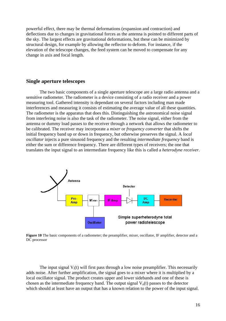
The two basic components of a single aperture telescope are a large radio antenna and asensitive radiometer. The radiometer is a device consisting of a radio receiver and a powermeasuring tool. Gathered intensity is dependant on several factors including man madeinterferences and measuring it consists of estimating the average value of all these quantities.The radiometer is the apparatus that does this. Distinguishing the astronomical noise signalfrom interfering noise is also the task of the radiometer. The noise signal, either from theantenna or dummy load passes to the receiver through a network that allows the radiometer tobe calibrated. The receiver may incorporate a mixer or frequency converter that shifts theinitial frequency band up or down in frequency, but otherwise preserves the signal. A localoscillator injects a pure sinusoid frequency and the resulting intermediate frequency band iseither the sum or difference frequency. There are different types of receivers; the one thattranslates the input signal to an intermediate frequency like this is called a heterodyne receiver.

Figure 10 The basic components of a radiometer; the preamplifier, mixer, oscillator, IF amplifier, detector and aDC processor

The input signal Vi(t) will first pass through a low noise preamplifier. This necessarilyadds noise. After further amplification, the signal goes to a mixer where it is multiplied by alocal oscillator signal. The product creates upper and lower sidebands and one of these ischosen as the intermediate frequency band. The output signal Vo(t) passes to the detectorwhich should at least have an output that has a known relation to the power of the input signal.

17

The average at time to lasting for integration time τ, is read out to the recorder. The randomnoise appearing at the output of an ideal radiometer will necessarily fluctuate with an rmsuncertainty given by equation (26). The power density received by an antenna of effective areaAeff, observing an unpolarized source of flux S, will be SA/2. When this power is expressed inunits of antenna temperature the limiting rms flux sensitivity for point source ∆S is

2 n

eff

kTS

A Bτ∆ = (27)

One sees therefore that the quotient Tn/Aeff is a measure of the sensitivity of a radio telescopesystem.

The antenna is analogous to the lens of an optical telescope. It gathers the radiation,transmits it to an electrical current and after processing, the radiation is measured. In the caseof radio telescopes, the antenna operates as a receiving device as opposed to a transmittingdevice. These two cases are actually equivalent because of time reversibility; solutions ofMaxwell’s equations are valid even when time is reversed. An antenna used for the purpose ofreceiving is considered for its receiving area, the so called effective area Aeff, an interceptedflux S and a yielded received power Prec . Effective area is directionally dependent, and is afunction of direction n , measured with respect to the antenna axis so that

rec effP A S= (28)

An antennas beamwidth is the range of directions over which Aeff operates. From lawsof diffraction; an antenna of size D will have a beamwidth of order λ/D. As a transmitter, thatsame antenna would have a power gain G(k) in a direction n , as opposed to an effective area.The power gain is the ratio of the radiated power flux S(k) that would be measured at somelarge distance, to the power flux from a hypothetical isotropic radiator, measured at the samedistance. For a transmitted power Ptr

2

ˆ(n)ˆ(n)4

trG PS

rπ= (29)

From the law of conservation of energy,

2

4ˆ(n) 4G d

ππΩ =∫ (30)

The antenna will concentrate the radiation into a principal beam of solid angle Ω0. For order ofmagnitude approximations this condition can be approximated by

04 /G π= Ω (31)

And since the beam will have a width λ/D, Aeff will be proportional to the power gain:

2 / 4effA Gλ π= (32)

18

Imagine an antenna enclosed by a blackbody with temperature T. The antenna isconnected to a transmission line, which is terminated by a matched load. This is a resistorhaving the same impedance as the line. Isolated from the outside world, the line and resistorwill reach an equilibrium temperature T, identical to that of the blackbody. The same radiofrequency power density Pν for any narrow band dν at frequency ν must flow in bothdirections along the transmission line. Planck’s distribution describes the radio density uν

3

3 /

8 11h kT

hu d d

c eν ν

π νν ν=

− (33)

In terms of specific intensity Bν (flux per frequency interval per solid angle):

3

2 /

2 11v h kT

hB d d

c e ν

νν ν=

− (34)

Using Rayleigh-Jeans approximation, that frequency lies below the Planck maximum,

2(2 / )B d kT dν ν λ ν= (35)

The corresponding derivation for noise power flowing in a single-mode transmission lineconnected to a blackbody at temperature T leads to the one-dimensional analogue of Planck’slaw

/ 1h kT

hP d d

eν ν

νν ν=

− (36)

Again with Rayleigh-Jeans approximation this reduces to

P d kTdν ν ν= , (37)

showing that within a given narrow band, noise power is proportional to temperature.

To relate the telescope aperture to the size and shape of the beam, we start withconsidering the antenna as a transmitter, bearing in mind the reciprocity between antennacharacteristics in reception and transmission. Imagine the aperture is a line distribution ofexcitation currents i(ξ) at a single wavelength λ. At a large distance, in direction θ to thenormal, the contribution of each element i(ξ)dξ to the radiation field depends on the phaseintroduced by the path ξ sin θ, the radiation pattern is F(θ):

( (2 / ))( ) ( )iF i de πξθ λθ ξ ξ−= ∫ , (38)

where normalizing factors have been omitted and the approximation sinθ=0 has been made. ξis measured in wavelengths and angles are measured as direction cosines l, m. Thegeneralization to a two dimensional aperture, where the distribution of current density isreferred to as grating, g(ξ,η) gives:

19

( 2 ( ))

4( , ) ( , ) ( , ) i

eF F g e d dπ ξθ ηφ

πθ φ θ φ ξ η ξ η− += ∫ ∫ , (39)

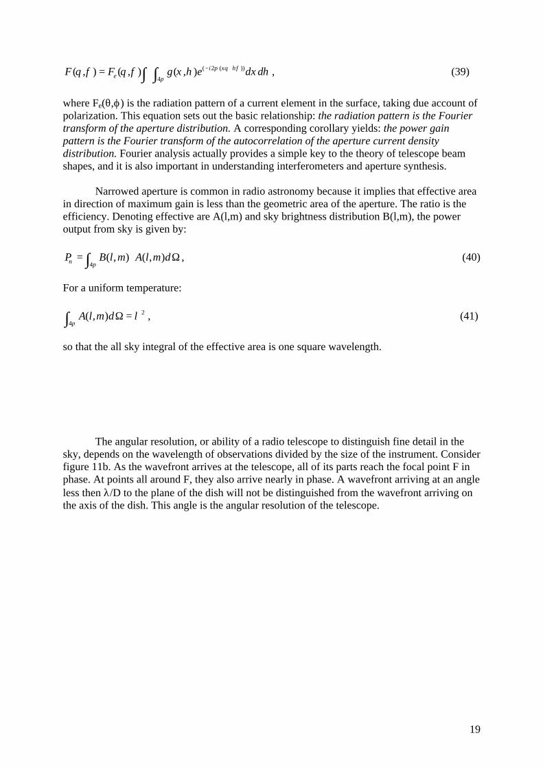
where Fe(θ,ϕ) is the radiation pattern of a current element in the surface, taking due account ofpolarization. This equation sets out the basic relationship: the radiation pattern is the Fouriertransform of the aperture distribution. A corresponding corollary yields: the power gainpattern is the Fourier transform of the autocorrelation of the aperture current densitydistribution. Fourier analysis actually provides a simple key to the theory of telescope beamshapes, and it is also important in understanding interferometers and aperture synthesis.

Narrowed aperture is common in radio astronomy because it implies that effective areain direction of maximum gain is less than the geometric area of the aperture. The ratio is theefficiency. Denoting effective are A(l,m) and sky brightness distribution B(l,m), the poweroutput from sky is given by:

4( , ) ( , )P B l m A l m dν π

= ⋅ Ω∫ , (40)

For a uniform temperature:

2

4( , )A l m d

πλΩ =∫ , (41)

so that the all sky integral of the effective area is one square wavelength.

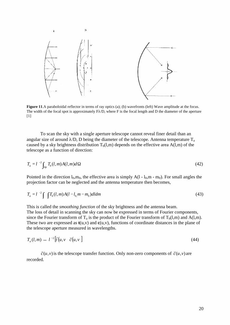
The angular resolution, or ability of a radio telescope to distinguish fine detail in thesky, depends on the wavelength of observations divided by the size of the instrument. Considerfigure 11b. As the wavefront arrives at the telescope, all of its parts reach the focal point F inphase. At points all around F, they also arrive nearly in phase. A wavefront arriving at an angleless then λ/D to the plane of the dish will not be distinguished from the wavefront arriving onthe axis of the dish. This angle is the angular resolution of the telescope.

20

Figure 11.A paraboloidal reflector in terms of ray optics (a); (b) wavefronts (left) Wave amplitude at the focus.The width of the focal spot is approximately Fλ/D, where F is the focal length and D the diameter of the aperture[1]

To scan the sky with a single aperture telescope cannot reveal finer detail than anangular size of around λ/D, D being the diameter of the telescope. Antenna temperature Ta

caused by a sky brightness distribution Tb(l,m) depends on the effective area A(l,m) of thetelescope as a function of direction:

2

4( , ) ( , )a bT T l m A l m d

πλ −= Ω∫ (42)

Pointed in the direction l0,m0, the effective area is simply A(l - l0,m - m0). For small angles theprojection factor can be neglected and the antenna temperature then becomes,

20, 0( , ) ( )a bT T l m A l l m m dldmλ −= − −∫ ∫ (43)

This is called the smoothing function of the sky brightness and the antenna beam.The loss of detail in scanning the sky can now be expressed in terms of Fourier components,since the Fourier transform of Ta is the product of the Fourier transform of Tb(l,m) and A(l,m).These two are expressed as t(u,v) and c(u,v), functions of coordinate distances in the plane ofthe telescope aperture measured in wavelengths.

( ) ( )[ ]vucvutmlTa ,,),( 2 rr⋅↔ −λ (44)

( , )c u vr

is the telescope transfer function. Only non-zero components of ( , )c u vr

arerecorded.

21

As mentioned, the efficiency of a radio telescope is can be limited by many factors andimperfections. Some example are deformations and irregularities on the surface which cancause errors in phase across the aperture. These phase imperfection transfer some power fromthe main beam in to the sidelobes. This represents a loss of efficiency. For a random Gaussiandistribution of phase error this loss is easily estimated. A portion of the wavefront with a smallphase error of φ radians makes a reduced concentration to the power in the main beam by a

fraction 1-φ 2, or more precisely2

e φ− ,and the contributions from the whole surface addrandomly. The phase error at a reflector with a surface error ε is 4πε/λ for normal reflection.Whole error is quoted as a single rms error ε, related to the surface efficiency ηsurf by theRuze formula:

(45)

Telescopes with a small angular resolutions are difficult to build, even the largestantennas, when used at their shortest operating wavelength, have an angular resolution only alittle better than one arc minute, which is almost the same as that of the human eye at opticalwavelengths. Because radio telescopes operate at much longer wavelengths than opticaltelescopes, they must be much larger than optical telescopes to achieve the same angularresolution. The angular resolution of a radio telescope used at given wavelength may beimproved by extending the dimensions of the aperture by adding extra elements in the form ofvarious types of interferometer.

Two-element interferometersInterference is the net effect of the combinations of two or more wavefronts moving on

coincident paths. The effect is that of the addition of the amplitudes of the individual waves ateach point of intersection. This can cause constructive or destructive interference. Twoelement interferometers consist of two widely separated antennas connected by transmissionlines. With their greatly increased resolving power, they can be used to determine the positionor diameter of a radio source or to separate two closely spaced sources. As the Earth rotatesfirst one and then the other will pass through antenna patterns. Their result is a superpositionof the total power from the source, modulated by a fringe pattern. Near the maximum of theantenna response it is sufficiently close to sinusoidal form to be characterized by its frequency,amplitude and phase. In such interferometers, the correlation between signal amplitudesreceived by two antenna elements is measured, in contrast to total power systems associatedwith single apertures.

2(4 / )surf e πε λη −=

22

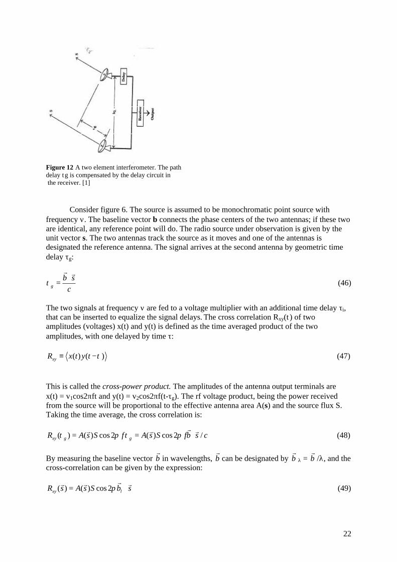
Figure 12 A two element interferometer. The pathdelay tg is compensated by the delay circuit in the receiver. [1]

Consider figure 6. The source is assumed to be monochromatic point source withfrequency ν. The baseline vector b connects the phase centers of the two antennas; if these twoare identical, any reference point will do. The radio source under observation is given by theunit vector s. The two antennas track the source as it moves and one of the antennas isdesignated the reference antenna. The signal arrives at the second antenna by geometric timedelay τg:

g

b sc

τ⋅

=r r

(46)

The two signals at frequency ν are fed to a voltage multiplier with an additional time delay τi,that can be inserted to equalize the signal delays. The cross correlation Rxy(t ) of twoamplitudes (voltages) x(t) and y(t) is defined as the time averaged product of the twoamplitudes, with one delayed by time τ:

( ) ( )xyR x t y t τ≡ − (47)

This is called the cross-power product. The amplitudes of the antenna output terminals arex(t) = v1cos2πft and y(t) = v2cos2πf(t-τg). The rf voltage product, being the power receivedfrom the source will be proportional to the effective antenna area A(s) and the source flux S.Taking the time average, the cross correlation is:

( ) ( ) cos 2 ( ) cos 2 /xy g gR A s S f A s S fb s cτ π τ π= = ⋅rr r r

(48)

By measuring the baseline vector br

in wavelengths, br

can be designated by br

λ = br

/λ, and thecross-correlation can be given by the expression:

( ) ( ) cos 2xyR s A s S b sλπ= ⋅rr r r

(49)

23

In either representation, the sinusoidal fringe variation is apparent. As the source directionchanges, the fringe amplitude oscillates and for spacing of many wavelengths, when the sourceis close to transit, the variations is nearly sinusoidal since b s bλ λ θ⋅ ≈

r rr. In this approximation,

with an angle θ between source and transit, and also making the assumption that the baseline isnearly perpendicular to the direction of observation:

( ) ( ) cos 2xyR A s S bλθ π θ= ⋅r

(50)

The angle between fringes in this small angle limit is 1/ bλ

r.

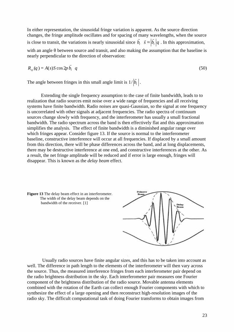
Extending the single frequency assumption to the case of finite bandwidth, leads to torealization that radio sources emit noise over a wide range of frequencies and all receivingsystems have finite bandwidth. Radio noises are quasi-Gaussian, so the signal at one frequencyis uncorrelated with other signals at adjacent frequencies. The radio spectra of continuumsources change slowly with frequency, and the interferometer has usually a small fractionalbandwidth. The radio spectrum across the band is then effectively flat and this approximationsimplifies the analysis. The effect of finite bandwidth is a diminished angular range overwhich fringes appear. Consider figure 13. If the source is normal to the interferometerbaseline, constructive interference will occur at all frequencies. If displaced by a small amountfrom this direction, there will be phase differences across the band, and at long displacements,there may be destructive interference at one end, and constructive interferences at the other. Asa result, the net fringe amplitude will be reduced and if error is large enough, fringes willdisappear. This is known as the delay beam effect.

Figure 13 The delay beam effect in an interferometer. The width of the delay beam depends on the bandwidth of the receiver. [1]

Usually radio sources have finite angular sizes, and this has to be taken into account aswell. The difference in path length to the elements of the interferometer will then vary acrossthe source. Thus, the measured interference fringes from each interferometer pair depend onthe radio brightness distribution in the sky. Each interferometer pair measures one Fouriercomponent of the brightness distribution of the radio source. Movable antenna elementscombined with the rotation of the Earth can collect enough Fourier components with which tosynthesize the effect of a large opening and then reconstruct high-resolution images of theradio sky. The difficult computational task of doing Fourier transforms to obtain images from

24

the interferometer data is accomplished with high-speed computers and the fast Fouriertransform (FFT), a mathematical technique especially designed for computing discrete Fouriertransforms.

Aperture Synthesis

It is possible to combine the data from two or more telescopes in such a way as toproduce an image whose detail is equivalent to a telescope whose diameter was equal to theseparation of the telescopes. Many antennas are linked electronically and the signals arerecorded. A computer then takes the data and synthesizes a map with as high resolution as wewould obtain if we were able to obtain a much larger dish.

Interferometer systems of almost unlimited element separation are formed by using thetechnique of very long baseline interferometry, or VLBI. In a VLBI system the signalsreceived at each element are recorded by broad-bandwidth videotape recorders located at eachelement. The recorded tapes are then transported to a common location where they arereplayed and the signals combined to form interference fringes. The successful operation of aVLBI system requires that the tape recordings be synchronized within a few millionths of asecond and that the local oscillator reference signal is stable to more than one part in a trillion.Normally, the analysis of the two-element interferometer can be generalized to the case of Nradio telescopes forming an aperture-synthesis array. For example, each pair of elements iscombined as an interferometer, and the correlator will evaluate the cross power product Rij forthe two voltage amplitudes as in (47). The geometric time delay τg must be compensated by aninstrumental time delay.

25

Conclusion

To fully understand how radio telescopes operate, complete knowledge of the theory onEM radiation and waves is required, as well as a deep insight into Fourier analysis. The latteris especially important when it comes to understanding how the telescopes detect andprocesses signals. Once the basics of the single aperture radio telescope are clear, it is easy toapply them to radio telescopes of many apertures. Finally, it is important to understand somebasic concepts behind the electronics of a radio telescope so that one can know how toconstruct and use them to obtain the best results possible.

26

[1]

27

28

29

30

31

32

33

References

[1] Burke B. F. and Graham-Smith F., An Introduction to Radio Astronomy, CambridgeUniversity Press, 1997, chapters 1-7 and appendices 1 and 3

[2] Rohlfs K. and Wilson T. L., Tools of Radio Astronomy, 4th ed., Springer, 2004, chapter4

[3] Freedman R. A. and Kaufmann W. J., Universe, 6th ed., Freeman and Company, 2002,chapter 6

[4] Griffiths David J., Introduction to electrodynamics, 3rd ed., Prentice Hall 1999, Chapters 9 and 11

[5] http://www.radiosky.com/simple.html

[6] http://www2.jpl.nasa.gov/radioastronomy/index.htm

[7] http://www.nrao.edu/

[8] http://www.lbl.gov/MicroWorlds/ALSTool/EMSpec/EMSpec2.html