Embed Size (px)
Citation preview
« The Precautionary Principle: An Economic Viewpoint »
Nicolas TreichToulouse School of Economics (LERNA-INRA & IDEI)[email protected]
Mabies, workshop ‘risk and learning in biodiversity management’04 March 2013
2
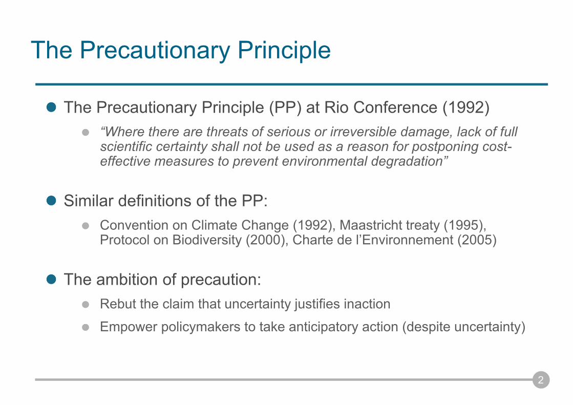
The Precautionary Principle
The Precautionary Principle (PP) at Rio Conference (1992)“Where there are threats of serious or irreversible damage, lack of full scientific certainty shall not be used as a reason for postponing cost-effective measures to prevent environmental degradation”
Similar definitions of the PP: Convention on Climate Change (1992), Maastricht treaty (1995), Protocol on Biodiversity (2000), Charte de l’Environnement (2005)
The ambition of precaution:Rebut the claim that uncertainty justifies inaction
Empower policymakers to take anticipatory action (despite uncertainty)

3
Motivation for the talk
An observation: Many qualitative discussions about the PP, both in academia and in practice, but few formal/quantitative approaches
Key questions:Can we give an economic interpretation to the PP?
Does scientific uncertainty justify more investments in safety?
This lecture is mostly a reflection about our economic modelsWhat do they mean? What do they imply?
4
A preview
Dealing with risk is not the same as dealing with uncertainty
The PP is related to a situation of uncertainty
Two main approaches in economics for dealing with uncertainty:One is based on the standard expected utility model
The other is based on ambiguity (aversion) models
Both approaches are problematic
5
Outline
1. Background on risk regulation and the PP
2. The expected utility model• Risk aversion, prudence, VSL, information value• Option values • Difficulties with the EU model
3. Ambiguity (aversion) models• The Ellsberg paradox• An ambiguity (aversion) model, and an application• Difficulties with ambiguity (aversion) models
1. Background on risk regulation and the PP
6
PP: Why so much fuss about a simple idea?
Precaution => be cautious« Better safe than sorry », « Look before you leap », « First do no harm », « Take care »
However, controversies :European Commission (2000, first sentence): « The issue of when and how to use the PP, both within the European Union and internationally, is giving rise to much debate, and to mixed, and sometimes contradictory views. »
7
Why do we need the PP now?
The effects of careless and harmful activities have accumulated over many decades of economicdevelopment
Earth limited capacity to absorb pollution
Plenty of warnings that suggest that we should nowproceed with caution
8
9
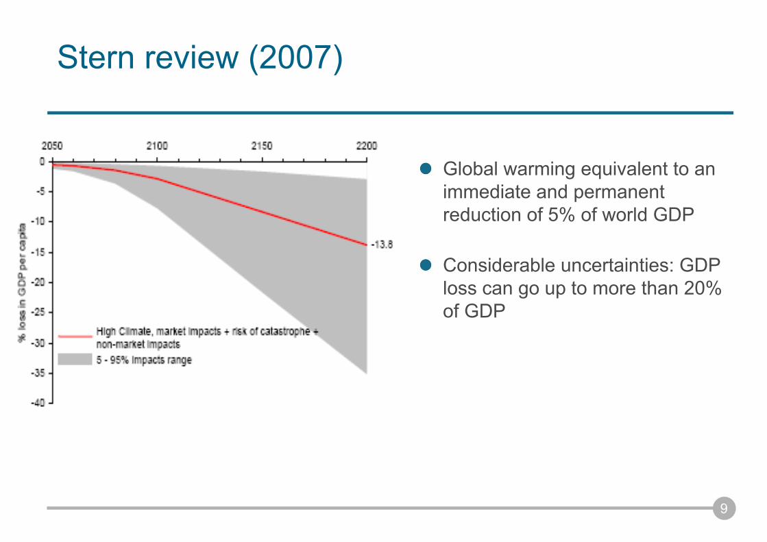
Stern review (2007)
Global warming equivalent to an immediate and permanent reduction of 5% of world GDP
Considerable uncertainties: GDP loss can go up to more than 20% of GDP
10
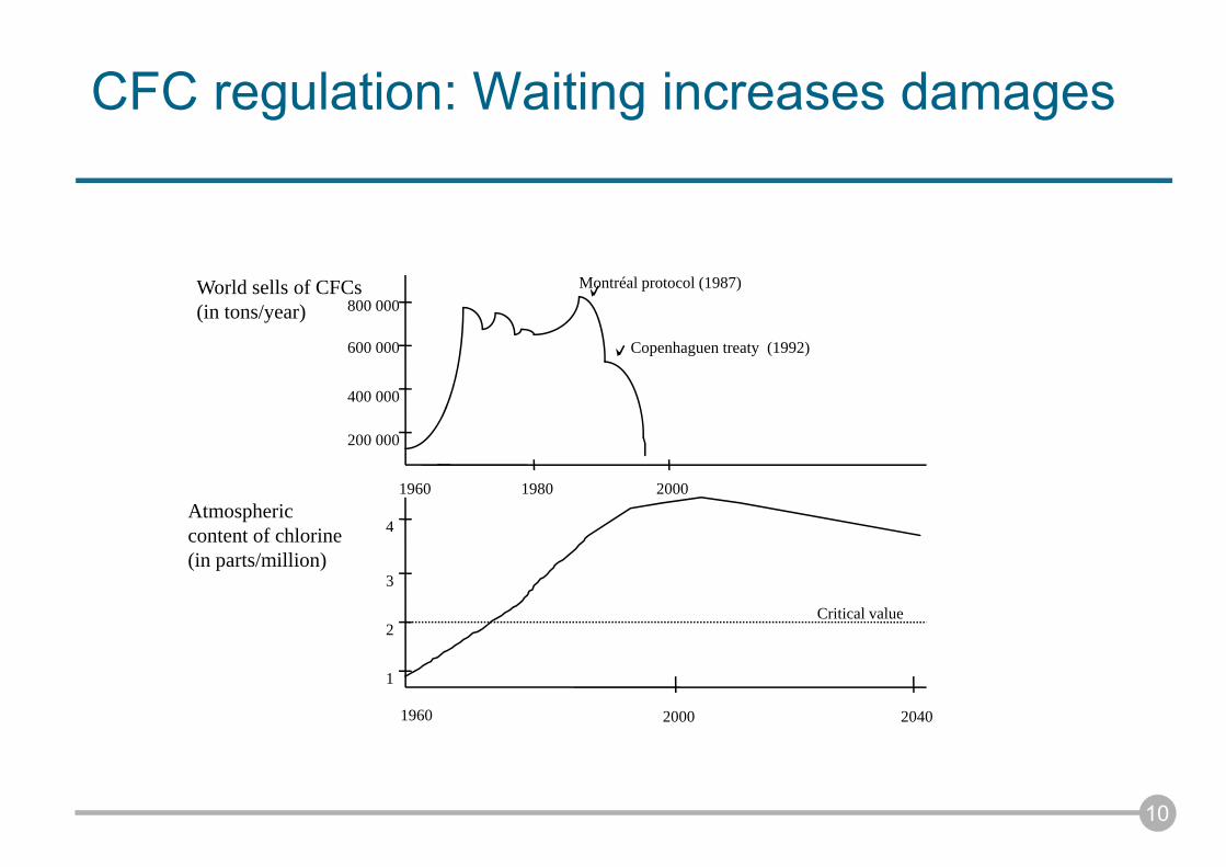
CFC regulation: Waiting increases damages
World sells of CFCs (in tons/year)
1960 2000
20401960 2000
200 000
400 000
600 000
800 000
1980
Montréal protocol (1987)
Copenhaguen treaty (1992)
1
2
3
4
Critical value
Atmosphericcontent of chlorine(in parts/million)
11
Emerging risks
High uncertainties
Large-scale effects
Long term effects
Stock and hysteresis effects
Physical irreversibilities
Socio-economic inertia
Scientific progress
12
Historical background on the PP
The PP has its roots, some believe, in the German DemocraticSocialism in the 1930s, centering on the concept of good householdmanagement (O’Riordan and Cameron 1994)
A precursor of the PP is known to be the German principle of « Vorsorge », or foresight, that was introduced in the early 1970s as an interventionist guideline for German environmental policy (Morris 2000, Sunstein 2005, Randall 2011)
It is often said that the PP was first applied in 1984 at the International Conference on Protection of the North Sea
Popular belief suggests that Europe is pro PP, and the US is against
13
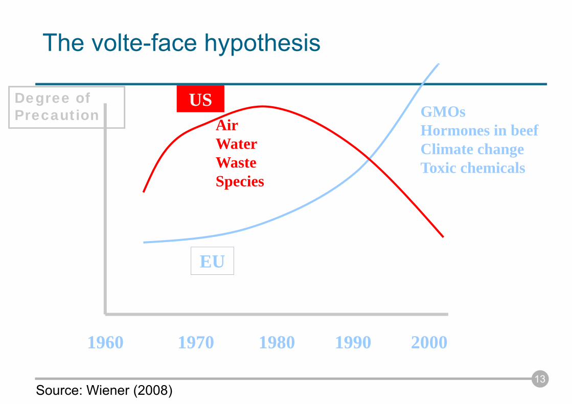
Degree of Precaution
1960 1970 1980 1990 2000
EU
USAirWaterWasteSpecies
GMOsHormones in beefClimate changeToxic chemicals
The volte-face hypothesis
Source: Wiener (2008)
14
Precaution is costly
An early example: the Superfund program in the US
Love Canal - Hazardous waste risk was ranked first concern by US citizens (but was ranked medium or low risk by experts)
Superfund: 36,000 sites, $50 billions, 50% of EPA budget in the 80s
Importance of political factors (Viscusi and Hamilton 1999, AER) and of “ad hoc” policy rules
On some sites, 5% of expenditures eliminated 99.5% of the risk (Hird 1994)
Cost per avoided cancer: >$1 billion!
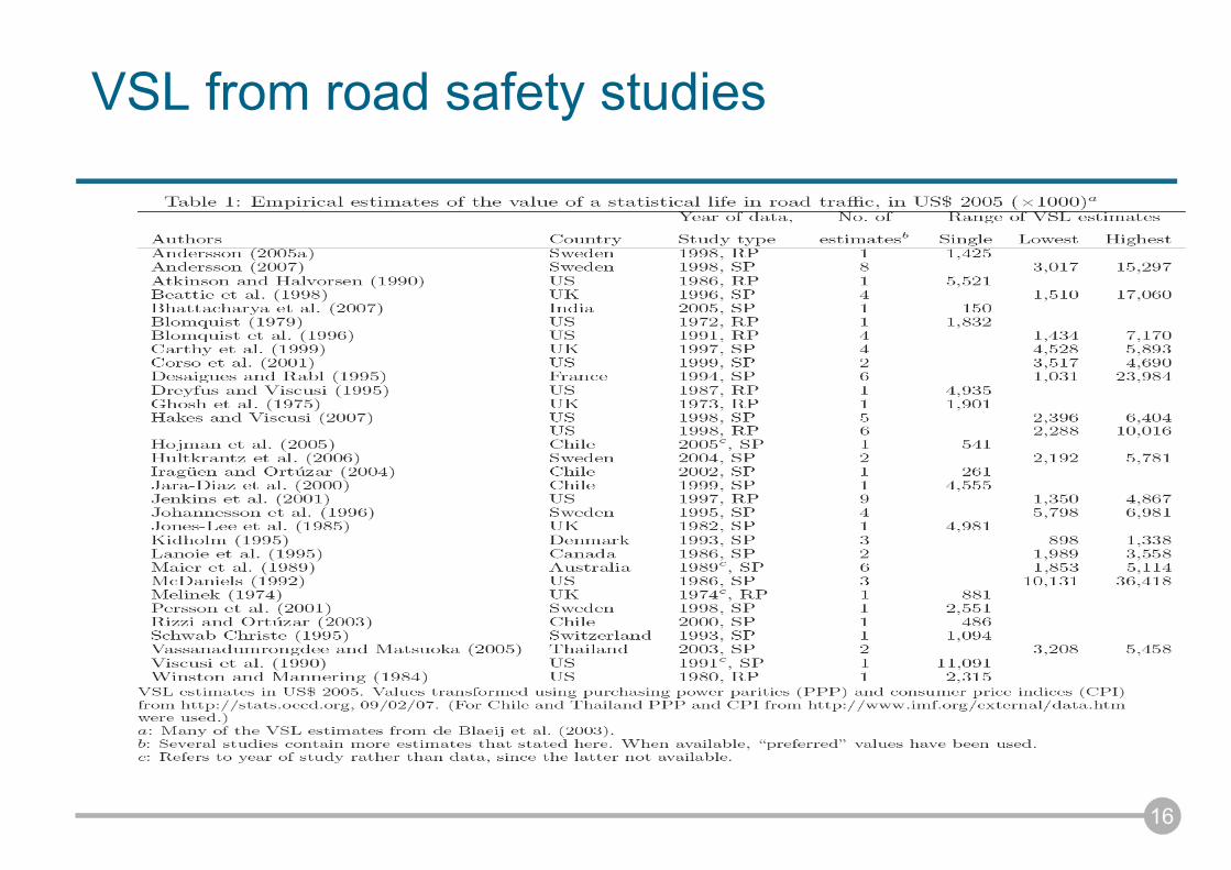
Inefficient since much larger than $1-10 million value-of-statistical-life (VSL) usually found in individual studies
15
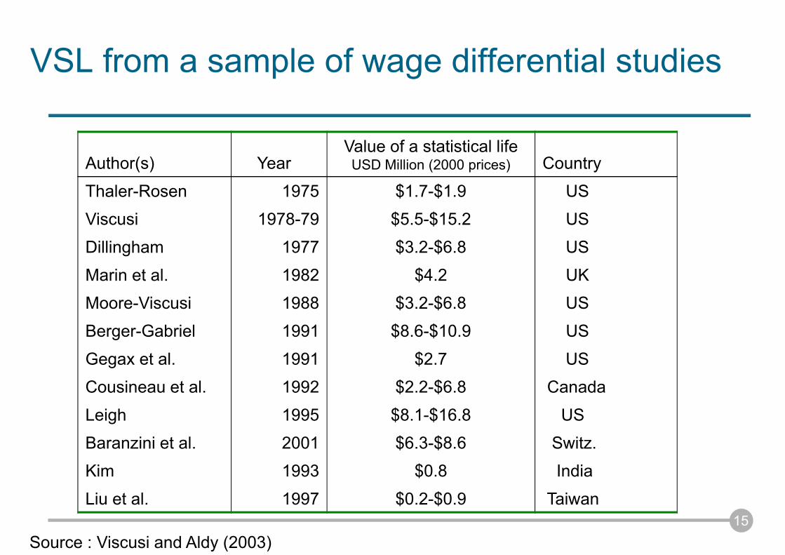
VSL from a sample of wage differential studies
Source : Viscusi and Aldy (2003)
Author(s) YearValue of a statistical lifeUSD Million (2000 prices) Country
Thaler-Rosen 1975 $1.7-$1.9 USViscusi 1978-79 $5.5-$15.2 US
Dillingham 1977 $3.2-$6.8 US
Marin et al. 1982 $4.2 UKMoore-Viscusi 1988 $3.2-$6.8 US
Berger-Gabriel 1991 $8.6-$10.9 US
Gegax et al. 1991 $2.7 USCousineau et al. 1992 $2.2-$6.8 Canada
Leigh 1995 $8.1-$16.8 US
Baranzini et al. 2001 $6.3-$8.6 Switz.Kim 1993 $0.8 India
Liu et al. 1997 $0.2-$0.9 Taiwan
16
VSL from road safety studies
17
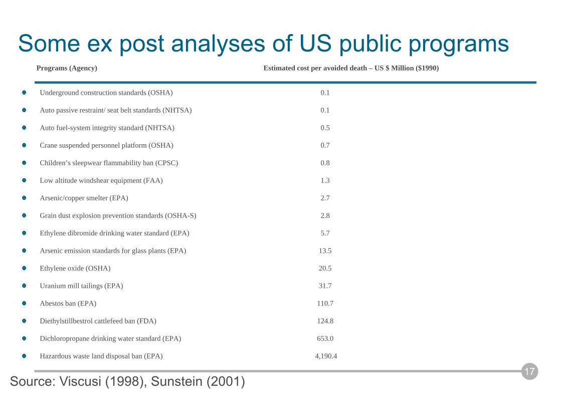
Some ex post analyses of US public programsPrograms (Agency) Estimated cost per avoided death – US $ Million ($1990)
Underground construction standards (OSHA) 0.1
Auto passive restraint/ seat belt standards (NHTSA) 0.1
Auto fuel-system integrity standard (NHTSA) 0.5
Crane suspended personnel platform (OSHA) 0.7
Children’s sleepwear flammability ban (CPSC) 0.8
Low altitude windshear equipment (FAA) 1.3
Arsenic/copper smelter (EPA) 2.7
Grain dust explosion prevention standards (OSHA-S) 2.8
Ethylene dibromide drinking water standard (EPA) 5.7
Arsenic emission standards for glass plants (EPA) 13.5
Ethylene oxide (OSHA) 20.5
Uranium mill tailings (EPA) 31.7
Abestos ban (EPA) 110.7
Diethylstillbestrol cattlefeed ban (FDA) 124.8
Dichloropropane drinking water standard (EPA) 653.0
Hazardous waste land disposal ban (EPA) 4,190.4
Source: Viscusi (1998), Sunstein (2001)
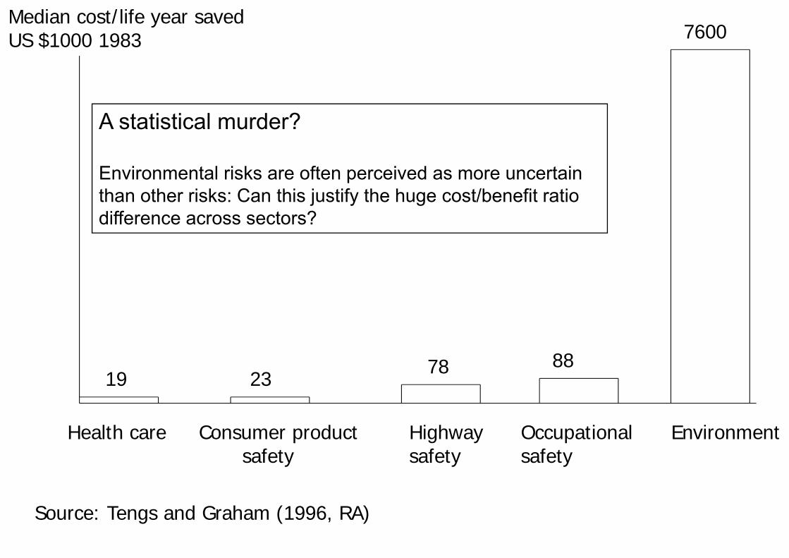
Median cost/life year savedUS $1000 1983
Health care Consumer productsafety
Highwaysafety
Occupational safety
Environment
19 2378 88
7600
Source: Tengs and Graham (1996, RA)
A statistical murder?
Environmental risks are often perceived as more uncertainthan other risks: Can this justify the huge cost/benefit ratio difference across sectors?
19
The PP = Laws of fear
Sunstein (2000) argues that policy-makers focus too much on the worst-case scenario, and the PP is mostly a demagogic response to citizens’ beliefs
People overestimate small risks
There is an uncertainty premium embodied in policy making (Viscusi1998; Sunstein 2000)
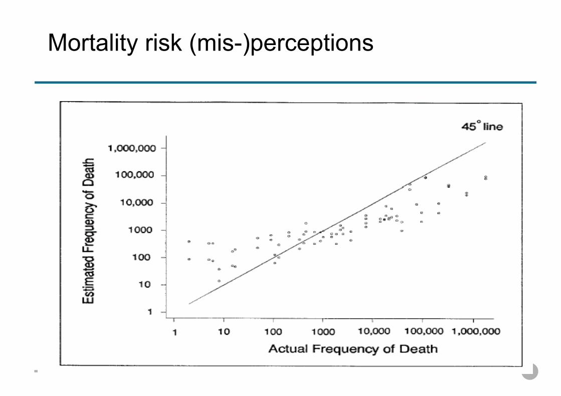
Mortality risk (mis-)perceptions
21
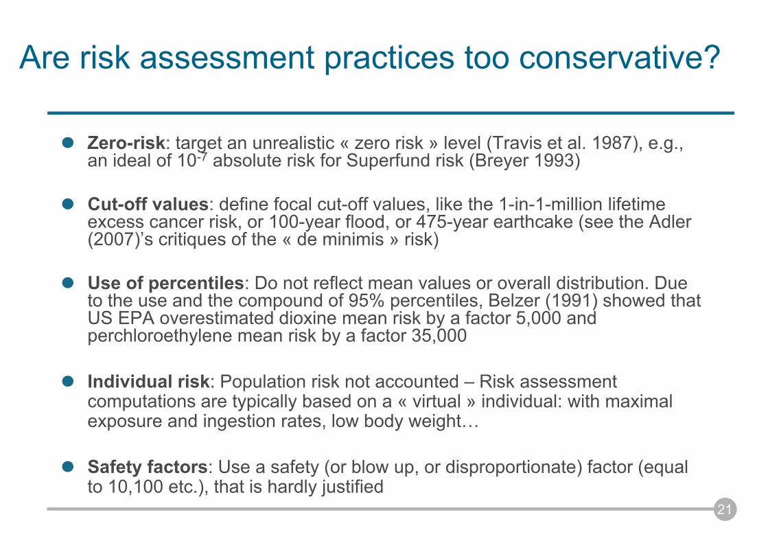
Zero-risk: target an unrealistic « zero risk » level (Travis et al. 1987), e.g., an ideal of 10-7 absolute risk for Superfund risk (Breyer 1993)
Cut-off values: define focal cut-off values, like the 1-in-1-million lifetime excess cancer risk, or 100-year flood, or 475-year earthcake (see the Adler (2007)’s critiques of the « de minimis » risk)
Use of percentiles: Do not reflect mean values or overall distribution. Due to the use and the compound of 95% percentiles, Belzer (1991) showed that US EPA overestimated dioxine mean risk by a factor 5,000 and perchloroethylene mean risk by a factor 35,000
Individual risk: Population risk not accounted – Risk assessment computations are typically based on a « virtual » individual: with maximal exposure and ingestion rates, low body weight…
Safety factors: Use a safety (or blow up, or disproportionate) factor (equal to 10,100 etc.), that is hardly justified
Are risk assessment practices too conservative?
22
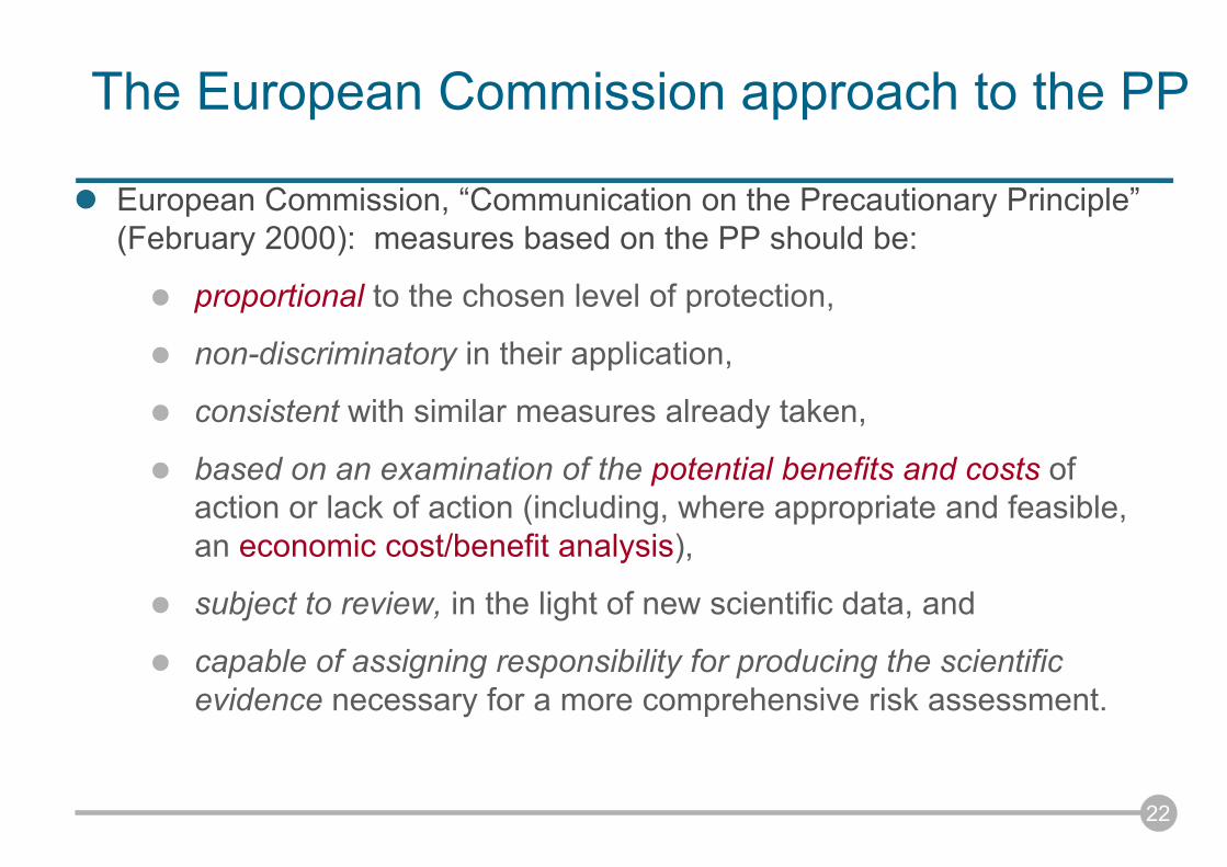
European Commission, “Communication on the Precautionary Principle” (February 2000): measures based on the PP should be:
proportional to the chosen level of protection,
non-discriminatory in their application,
consistent with similar measures already taken,
based on an examination of the potential benefits and costs of action or lack of action (including, where appropriate and feasible, an economic cost/benefit analysis),
subject to review, in the light of new scientific data, and
capable of assigning responsibility for producing the scientific evidence necessary for a more comprehensive risk assessment.
The European Commission approach to the PP
2. The Expected Utility Model
Risk versus uncertainty
The Savage Framework
Risk aversion, and prudence
Models of option values
23
24
Knight and Keynes’ early contributions
Knight (1921) is often credited as the first writer to make a distinction between risk and uncertainty
« Uncertainty must be taken in a sense radically distinct from the familiar notion of Risk, from which it has never been properly separated. . . A measurable uncertainty(i.e. risk) . . . .is so different from an immeasurable one that it is not in effect an uncertainty at all. »
Keynes (1921 – initiated in his master thesis 1908)
Argues that propositions and events vary in their « appropriate degree of rational belief ». Keynes discusses the concept of « confidence in beliefs » and, although hedid not believe that this need to be numerically scaled, he was concerned in the comparison of « degrees of beliefs ». See discussions in Jones and Ostroy (1984) and O’Donnell (1989).
25
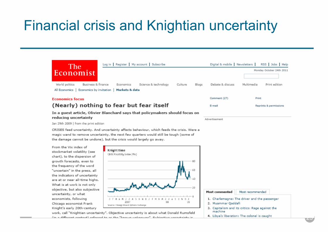
Financial crisis and Knightian uncertainty
What is a probability?
Traditionnally, three views of a probability:frequentist
logical
subjectivist
The subjectivist’s view can be summarized by the famous De Finetti (1928)’s sentence: « probability does not exist »
This sentence means that an « objective » probability does not exist, a probability only exists in the mind of individuals, it is a « degree of belief », and is thus subjective
De Finetti as well as Savage (1954) propose a behavioraldefinition of probability, measured by the willingness to bet
26
The Savage expected utility (EU) framework
The von Neumann-Morgenstern EU framework is based on objective probabilities, so it is implicitly « frequentist » or « logical »,
Savage (1954) axiomatize EU with subjective probabilities
In the Savage framework, there is no difference between risk and uncertainty
In the Savage framework, probabilities can be anything (since theyare subjective)
There is thus no sense to talk about « right » or « wrong » beliefs, more pessismistic, or biased beliefsThis view has been criticized: “[U]tilities directly express tastes, which are inherently personal. It would be silly to talk about impersonal tastes, tastes that are objective or unbiased. But it is not at all silly to talk about unbiased probability estimates, and even to strive to achieve them.” (Aumann 1987)
27
28
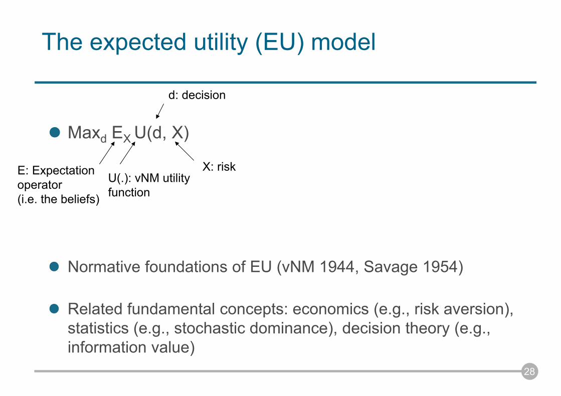
The expected utility (EU) model
Maxd EX U(d, X)
Normative foundations of EU (vNM 1944, Savage 1954)
Related fundamental concepts: economics (e.g., risk aversion), statistics (e.g., stochastic dominance), decision theory (e.g., information value)
U(.): vNM utilityfunction
d: decision
X: riskE: Expectationoperator(i.e. the beliefs)
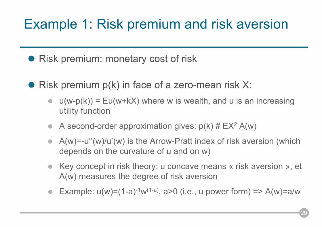
Example 1: Risk premium and risk aversion
Risk premium: monetary cost of risk
Risk premium p(k) in face of a zero-mean risk X:u(w-p(k)) = Eu(w+kX) where w is wealth, and u is an increasingutility function
A second-order approximation gives: p(k) # EX2 A(w)
A(w)=-u’’(w)/u’(w) is the Arrow-Pratt index of risk aversion (whichdepends on the curvature of u and on w)
Key concept in risk theory: u concave means « risk aversion », et A(w) measures the degree of risk aversion
Example: u(w)=(1-a)-1w(1-a), a>0 (i.e., u power form) => A(w)=a/w
29
30
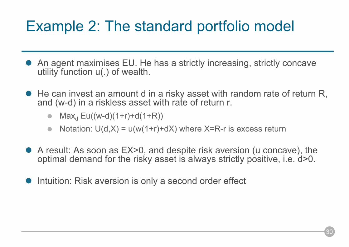
Example 2: The standard portfolio model
An agent maximises EU. He has a strictly increasing, strictly concave utility function u(.) of wealth.
He can invest an amount d in a risky asset with random rate of return R, and (w-d) in a riskless asset with rate of return r.
Maxd Eu((w-d)(1+r)+d(1+R))Notation: U(d,X) = u(w(1+r)+dX) where X=R-r is excess return
A result: As soon as EX>0, and despite risk aversion (u concave), the optimal demand for the risky asset is always strictly positive, i.e. d>0.
Intuition: Risk aversion is only a second order effect
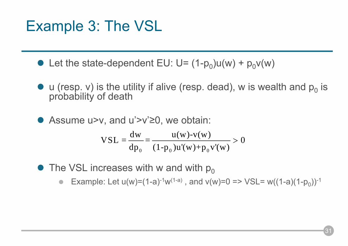
Example 3: The VSL
Let the state-dependent EU: U= (1-p0)u(w) + p0v(w)
u (resp. v) is the utility if alive (resp. dead), w is wealth and p0 isprobability of death
Assume u>v, and u’>v’≥0, we obtain:
The VSL increases with w and with p0Example: Let u(w)=(1-a)-1w(1-a) , and v(w)=0 => VSL= w((1-a)(1-p0))-1
31
0 0 0
dw u(w)-v(w)VSL = = 0dp (1-p )u'(w)+p v'(w)
32
Example 4: Precautionary savings
Two-period model with wealth w1 and w2 in each period. How to allocate consumption across periods?
d*= arg Maxd u(w1-d) + v(w2 + d(1+r))
d** = arg Maxd u(w1-d) + Ev(w2 + d(1+r)+ X) with EX=0 (future income is risky)
Precautionary savings iff d**>d*. Induced by risk aversion?
No! For all X, we have d**>d* iff v’’’(.)>0 (Leland 1968, Kimball 1990). Condition v’’’(.) is coined « prudence ».
33
Example 5: Information value (IV)
Simple investment decision problem under risk neutrality (i.e. linear utility function)
U(d,X)= d (X-c) with d in {0,1} [interpretation: c is cost and X is unknown benefit]
Investment rule: invest (i.e., d=1) iff EX>c. Expected profit: max(EX-c, 0)
Suppose now perfect information is expected (i.e., a message will give perfectinformation about the realization of X).
Investment rule: invest iff X=x>c. Expected profit: Emax(X-c,0)
Information Value: IV=Emax(X-c,0) - max(EX-c, 0) ≥0
Example:
Take: c=100, X=(50%, 200, 50%, 50). IV= 50-25=25
Take: c=100, X=(50%, 140, 50%, 50). IV= 20-0=20
34
An exercise: Park vs. parking
Consider the choice between i) preserving a park or ii) building a parking
There are two periods (present and future), and the discount rate is assumedto equal zero (to simplify)
The costs and benefits have been estimated by our best experts
The parking yields $40 benefit in each period, and the construction cost is $25
The park yields $0 benefit in period 1, and either $100 or $0 in period 2 withequal probability
Based on benefit cost analysis (BCA), the parking is built (since it yields $55 net benefit > the net expected benefit of the park $50)
Do you agree with this choice in favor of the irreversible decision?
35
The option value
The value of preserving the park is in fact $57.5, and is therefore the best decision
Compared to standard BCA, there is an additional value of $7.5, coinedthe (quasi-)option value, that leads to preserve the park
This is the value of flexibility: building the parking is irreversible whilepreserving the park is flexible since it maintains both options in the future
The option value is consistent with the PP: scientific uncertainty shouldlead to preserve flexibility
Early contributions on option values: Arrow and Fisher (1974, QJE), Henry (1974, AER), Epstein (1980, IER), Jones and Ostroy (1984, RES)
36
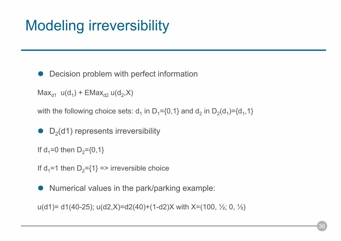
Modeling irreversibility
Decision problem with perfect information
Maxd1 u(d1) + EMaxd2 u(d2,X)
with the following choice sets: d1 in D1={0,1} and d2 in D2(d1)={d1,1}
D2(d1) represents irreversibility
If d1=0 then D2={0,1}
If d1=1 then D2={1} => irreversible choice
Numerical values in the park/parking example:
u(d1)= d1(40-25); u(d2,X)=d2(40)+(1-d2)X with X=(100, ½; 0, ½)
37
Information and optimal timing in policy-making
Information/timing is critical for policy-making:What should I do today given that I will have better information in the future? Should I delay decisions? Should I be more cautious?
« The challenge is not to find the best policy today for the next 100 years, but to select a prudent and flexible strategy and to adjust it over time » (IPCC 1995)
« Measures should be periodically reviewed in the light of scientific progress, and amended as necessary" » (European Commission 2000)
38
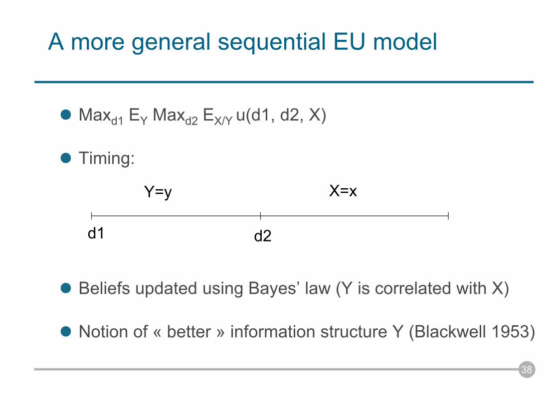
A more general sequential EU model
Maxd1 EY Maxd2 EX/Y u(d1, d2, X)
Timing:
Beliefs updated using Bayes’ law (Y is correlated with X)
Notion of « better » information structure Y (Blackwell 1953)
d1 d2
X=xY=y
39
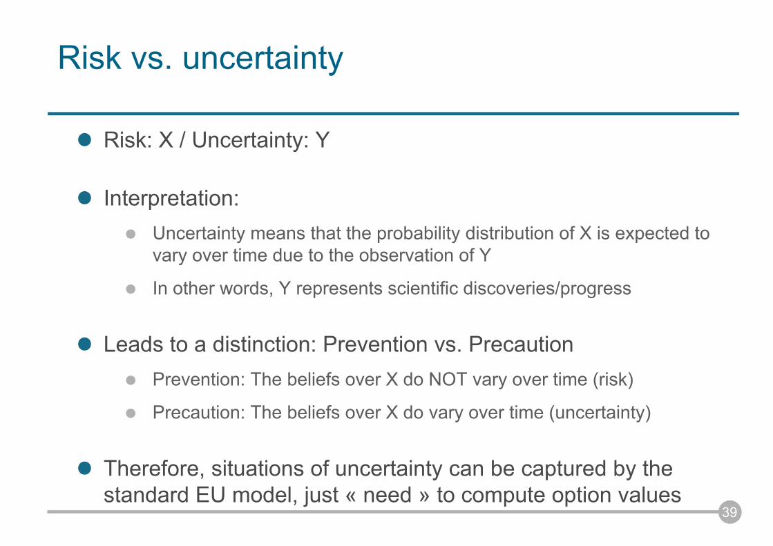
Risk vs. uncertainty
Risk: X / Uncertainty: Y
Interpretation: Uncertainty means that the probability distribution of X is expected to vary over time due to the observation of Y
In other words, Y represents scientific discoveries/progress
Leads to a distinction: Prevention vs. PrecautionPrevention: The beliefs over X do NOT vary over time (risk)
Precaution: The beliefs over X do vary over time (uncertainty)
Therefore, situations of uncertainty can be captured by the standard EU model, just « need » to compute option values
Let us summarize
Remember the definition of the PP
“Where there are threats of serious or irreversible damage, lack of full scientific certainty shall not be used as a reason for postponing cost-effective measures to prevent environmental degradation” (Rio Conference 1992)
We have shown:
That the lack of full scientific uncertainty can be modeled within an EU bayesian model by the prospect to receive information over time (i.e. Y).
Key question in order to justify the PP: Does the prospect to receiveinformation should always lead us to be more cautious in the short run?
40
41
An economic interpretation of the PP
Gollier, Jullien and Treich (2000, JPubE)U(d1,d2,X) = u(d1) + v(d2 – X (d1+d2))
Decisions d1 and d2 can be interpreted as the consumption of a toxicproduct (e.g., consumption of energy emitting CO2 emissions)
Includes stock/hysteresis effects in the simple option value model => much more compelx
42
An economic interpretation of the PP (cont’d)
The model shows that it is justified to reduce the first-perioddecision d1 with a better information Y only for specific utility functions; namely, only when v is « sufficiently prudent »
Scientific message: The PP is not always justifiedeconomically; this depends on risk preferences
Intuition: Two opposite effects, i.e.,i) better to wait for information before acting,
ii) better to act early to maintain « cheap » options available
43
Option value in benefit-cost analysis (BCA)
Can the option value make a difference in practical BCA?« Potentially, yes. (…) Delay can improve the quality of the decision. Further study is needed » Pearce et al. (2006)
An example is Nordhaus (1994) for climate policy, but showing thatthe option value of delaying abatement is small
Note that it is difficult to compute option values: Requires a full representation of uncertainties, and of how they mightbe resolved over time
Requires to capture the various degrees of flexibility/irreversibility
44
Difficulties with this standard EU approach
In practiceTechnically difficult to compute option values. « Examples to date are limited » (Pearce et al. 2006, OECD).
In lab experiments
Subjects do not maximize EU, and are not bayesian (Allais 1953, Kahneman and Tversky 1979, Camerer 1995)
On normative grounds
EU does not seem to account well for the coexistence of multiple priors
45
Monty Hall paradox
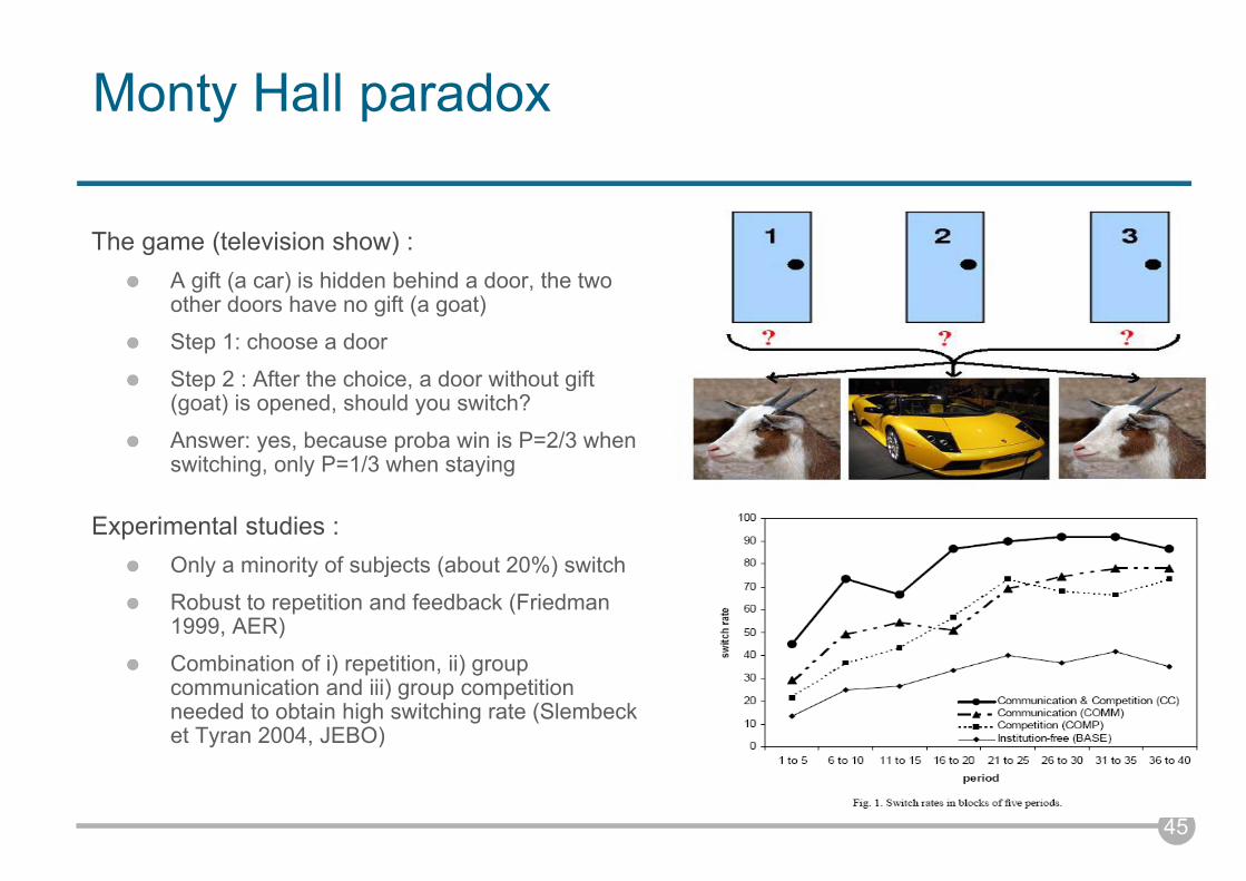
The game (television show) : A gift (a car) is hidden behind a door, the twoother doors have no gift (a goat)
Step 1: choose a door
Step 2 : After the choice, a door without gift (goat) is opened, should you switch?
Answer: yes, because proba win is P=2/3 whenswitching, only P=1/3 when staying
Experimental studies : Only a minority of subjects (about 20%) switch
Robust to repetition and feedback (Friedman 1999, AER)
Combination of i) repetition, ii) group communication and iii) group competitionneeded to obtain high switching rate (Slembecket Tyran 2004, JEBO)
3. Ambiguity (Aversion) Models
The Ellsberg paradox
A model of ambiguity (aversion)
An application: Ambiguity aversion and the VSL
Difficulties with ambiguity (aversion) models
46
47
Ambiguity and climate sensitivity
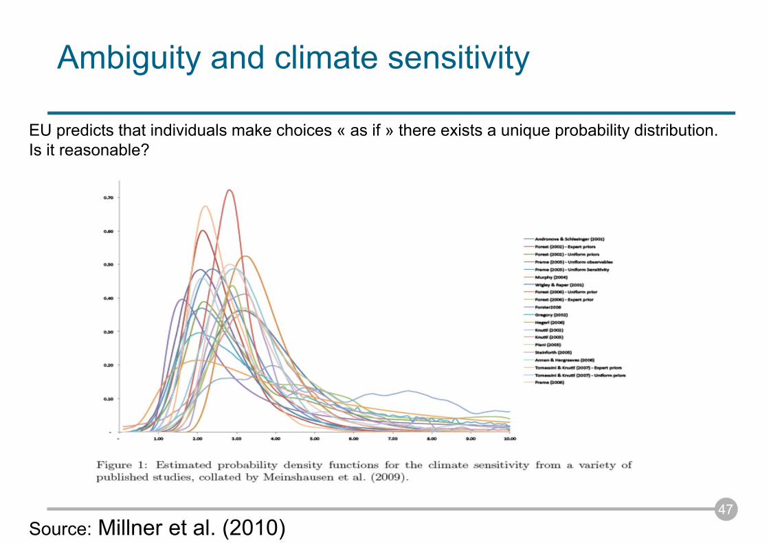
EU predicts that individuals make choices « as if » there exists a unique probability distribution. Is it reasonable?
Source: Millner et al. (2010)
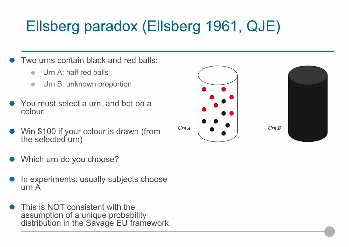
Ellsberg paradox (Ellsberg 1961, QJE)
Two urns contain black and red balls: Urn A: half red ballsUrn B: unknown proportion
You must select a urn, and bet on a colour
Win $100 if your colour is drawn (fromthe selected urn)
Which urn do you choose?
In experiments: usually subjects chooseurn A
This is NOT consistent with the assumption of a unique probabilitydistribution in the Savage EU framework
49
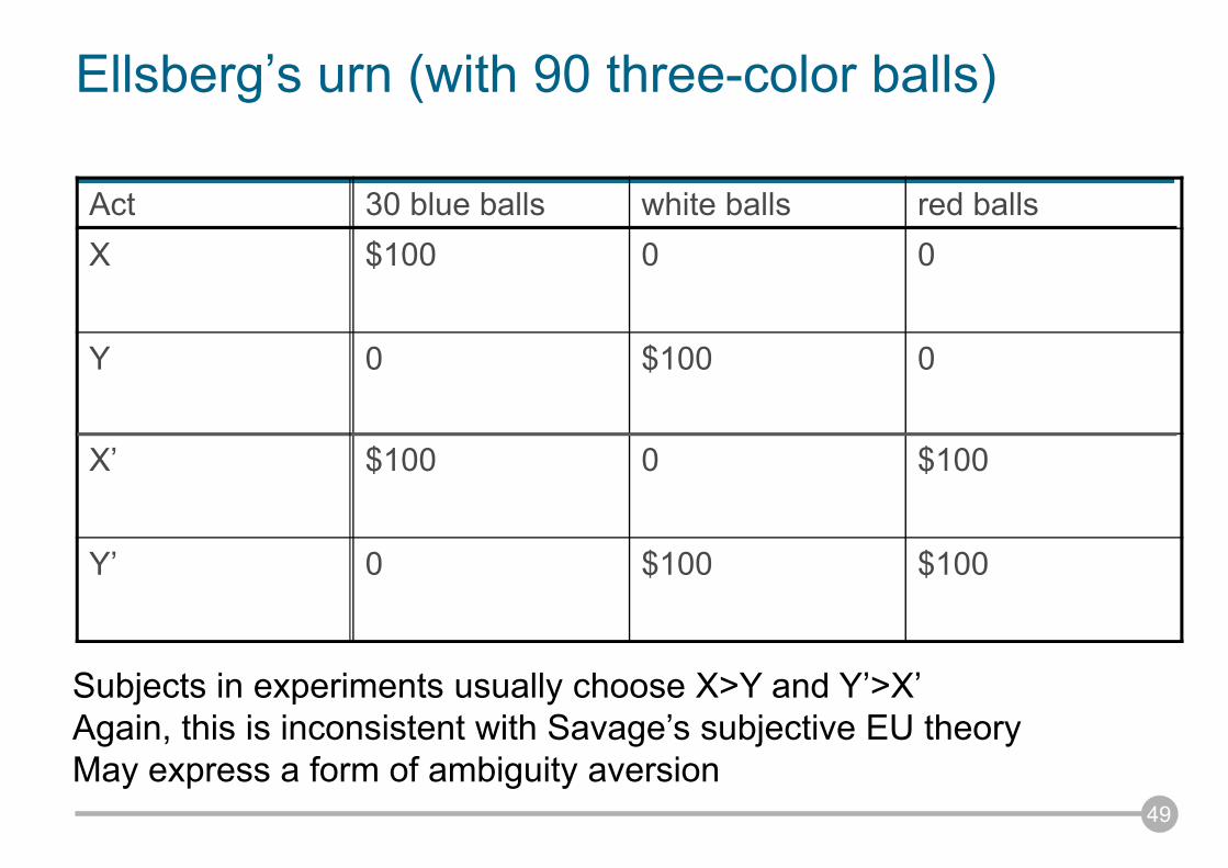
Ellsberg’s urn (with 90 three-color balls)
Act 30 blue balls white balls red ballsX $100 0 0
Y 0 $100 0
X’ $100 0 $100
Y’ 0 $100 $100
Subjects in experiments usually choose X>Y and Y’>X’Again, this is inconsistent with Savage’s subjective EU theoryMay express a form of ambiguity aversion
50
Ambiguity aversion literature
Subjects have often been found to be averse to ambiguousprobabilities
A wealth of experimental evidence (e.g., Camerer and Weber 1992)
Survey evidence (Hogarth and Kunreuther 1985; Viscusi et al. 1991; Chesson and Viscusi 2003; Burks et al. 2008)
Remark: almost no empirical evidence about ambiguity aversion
Theoretical applications: ambiguity aversion may explain someempirical puzzle in finance (Dow and Werlang 1992; Mukerjiand Tallon 2001; Chen and Epstein 2002; Ju and Miao 2009; Epstein and Schneider 2010)
Causes to ambiguity aversion?
An deeper level of rationality in front of uncertainty: “Agents can have different models (..) and be aware of the possibility that their model is mis-specified” (Maccheroni et al. 1995)
Paranoia: the decision-maker behaves as if a malevolent Nature changes the odds against him (Cerreia et al. 2008)
Fear: Using brain imaging, Camerer et al. (2007) find evidencethat the amygdala is more active under ambiguity conditions, and notice that the “amygdala has been specifically implicated in processing information related to fear”
51
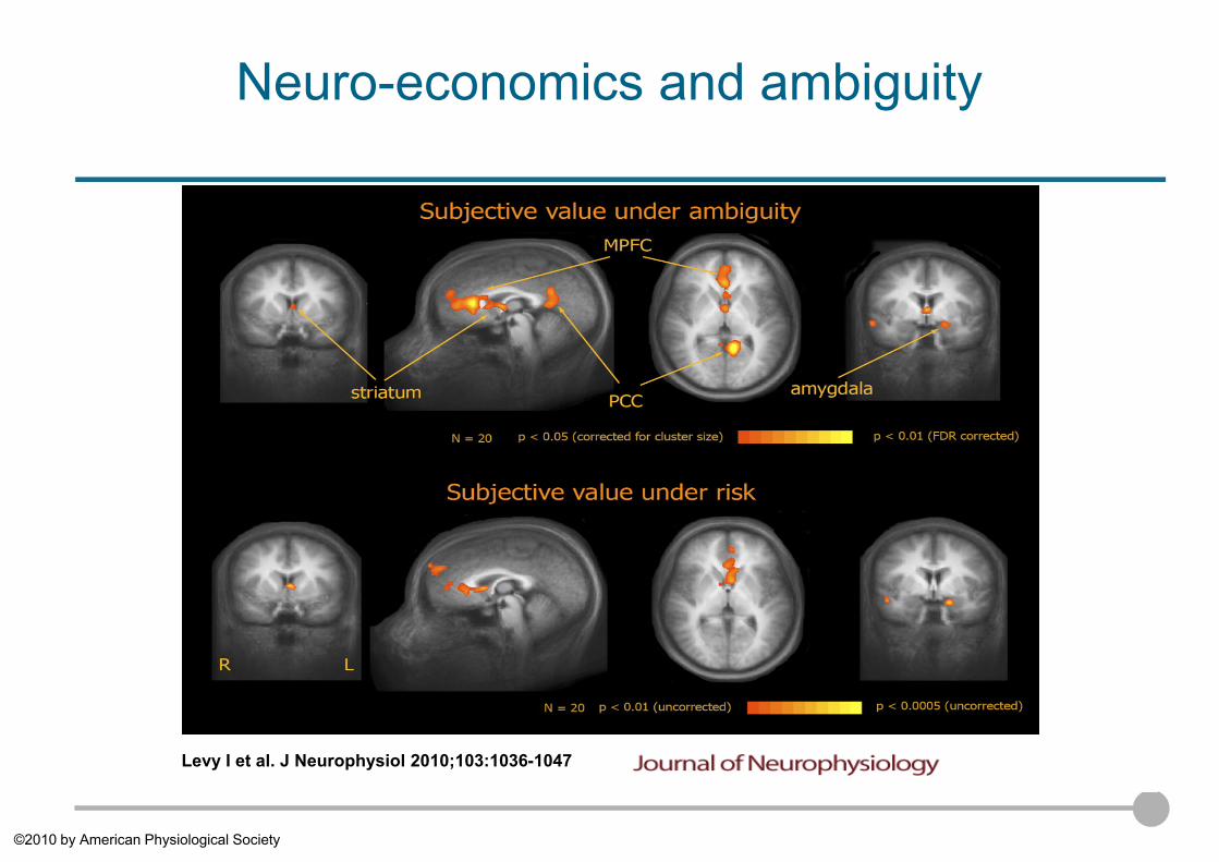
Neuro-economics and ambiguity
Levy I et al. J Neurophysiol 2010;103:1036-1047
©2010 by American Physiological Society
53
Modeling ambiguity aversion
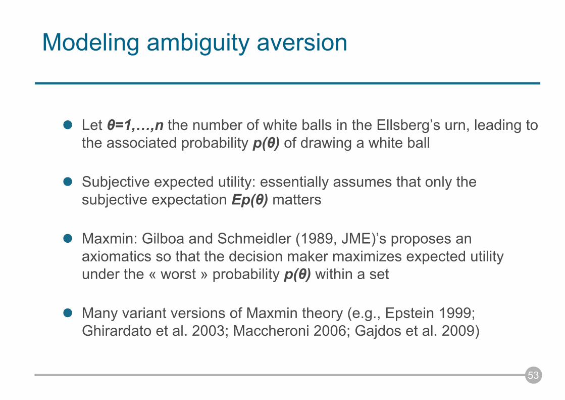
Let θ=1,…,n the number of white balls in the Ellsberg’s urn, leading to the associated probability p(θ) of drawing a white ball
Subjective expected utility: essentially assumes that only the subjective expectation Ep(θ) matters
Maxmin: Gilboa and Schmeidler (1989, JME)’s proposes an axiomatics so that the decision maker maximizes expected utility under the « worst » probability p(θ) within a set
Many variant versions of Maxmin theory (e.g., Epstein 1999; Ghirardato et al. 2003; Maccheroni 2006; Gajdos et al. 2009)
54
A popular model of ambiguity aversion
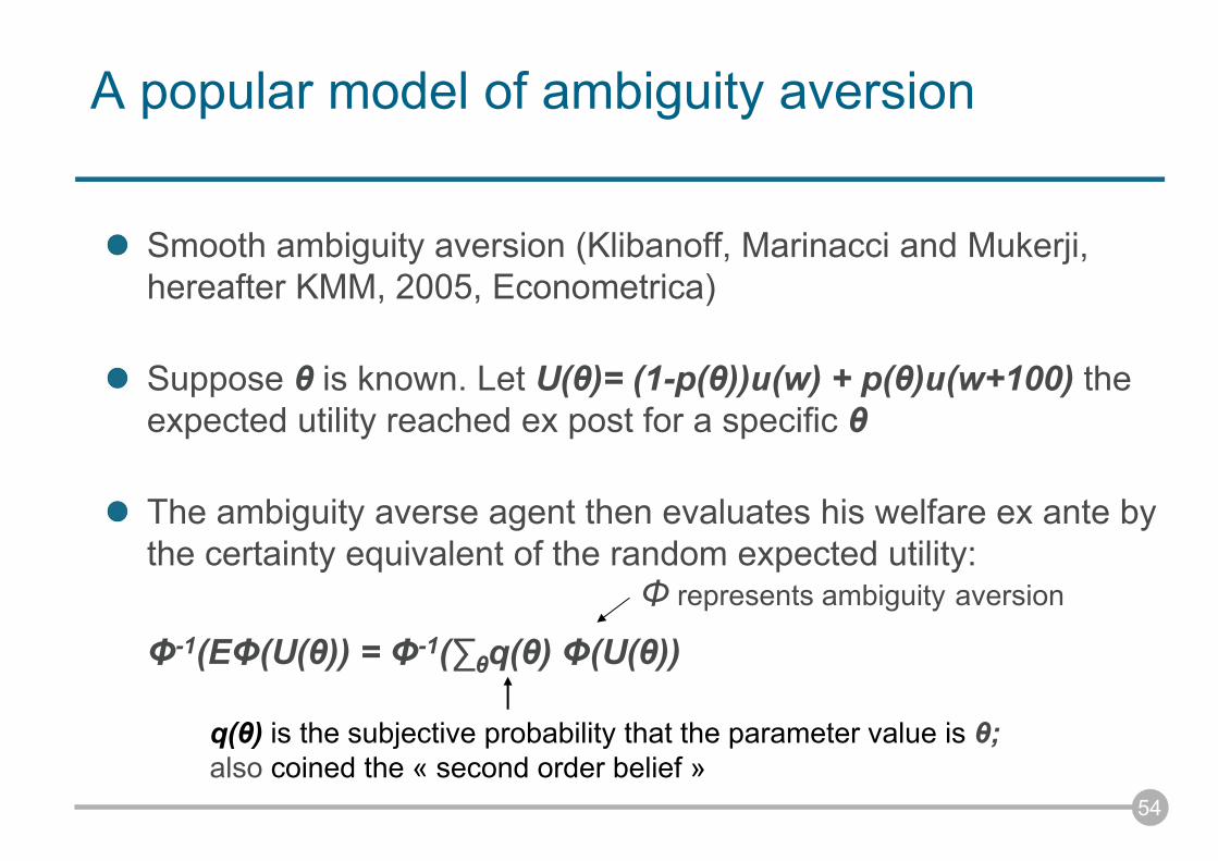
Smooth ambiguity aversion (Klibanoff, Marinacci and Mukerji, hereafter KMM, 2005, Econometrica)
Suppose θ is known. Let U(θ)= (1-p(θ))u(w) + p(θ)u(w+100) the expected utility reached ex post for a specific θ
The ambiguity averse agent then evaluates his welfare ex ante by the certainty equivalent of the random expected utility:
Φ-1(EΦ(U(θ)) = Φ-1(∑θq(θ) Φ(U(θ))
q(θ) is the subjective probability that the parameter value is θ;also coined the « second order belief »
Φ represents ambiguity aversion
55
KMM preferences
Interpretation: two-stage lottery (first-stage determining probabilitydistribution, and second-stage determining outcome)
Axiomatics: unique second order belief giving rise to an expectation over EU
Distinguish ambiguity, ambiguity aversion (a concave ø), and Arrow-Pratt risk aversion – moreover defines an « index » of ambiguity aversion
Two benchmarks: expected utility for ø linear, and MaxMin of Gilboa-Schmeidler (1989) for ø CARA with infinite absolute risk aversion
Open to a violation of the axiom of reduction of compound lotteries for ønon-linear (see Segal 1987; see also Kreps and Porteus 1978)
Preferences are not « kinked » (as with MaxMin) but are « smooth » when ø is differentiable, thus improving mathematical tractability
56
An application of ambiguity aversion: the VSL
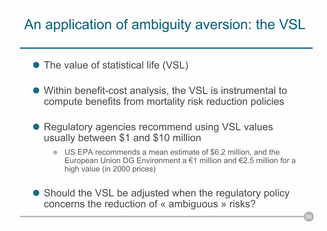
The value of statistical life (VSL)
Within benefit-cost analysis, the VSL is instrumental to compute benefits from mortality risk reduction policies
Regulatory agencies recommend using VSL values usually between $1 and $10 million
US EPA recommends a mean estimate of $6.2 million, and the European Union DG Environment a €1 million and €2.5 million for a high value (in 2000 prices)
Should the VSL be adjusted when the regulatory policyconcerns the reduction of « ambiguous » risks?
57
The VSL concept – introductory example
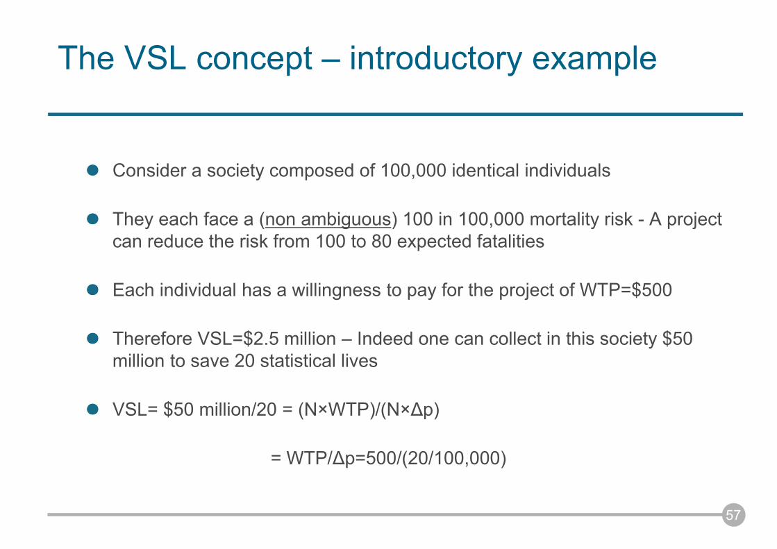
Consider a society composed of 100,000 identical individuals
They each face a (non ambiguous) 100 in 100,000 mortality risk - A project can reduce the risk from 100 to 80 expected fatalities
Each individual has a willingness to pay for the project of WTP=$500
Therefore VSL=$2.5 million – Indeed one can collect in this society $50 million to save 20 statistical lives
VSL= $50 million/20 = (N×WTP)/(N×∆p)
= WTP/∆p=500/(20/100,000)
58
The VSL concept – underlying framework
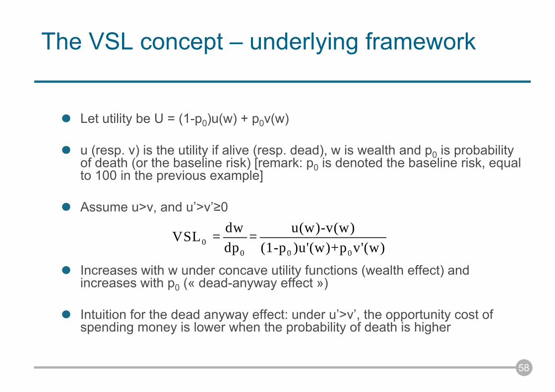
Let utility be U = (1-p0)u(w) + p0v(w)
u (resp. v) is the utility if alive (resp. dead), w is wealth and p0 is probabilityof death (or the baseline risk) [remark: p0 is denoted the baseline risk, equalto 100 in the previous example]
Assume u>v, and u’>v’≥0
Increases with w under concave utility functions (wealth effect) and increases with p0 (« dead-anyway effect »)
Intuition for the dead anyway effect: under u’>v’, the opportunity cost of spending money is lower when the probability of death is higher
00 0 0
dw u(w)-v(w)VSL = =dp (1-p )u'(w)+p v'(w)
59
A VSL model with ambiguity aversion
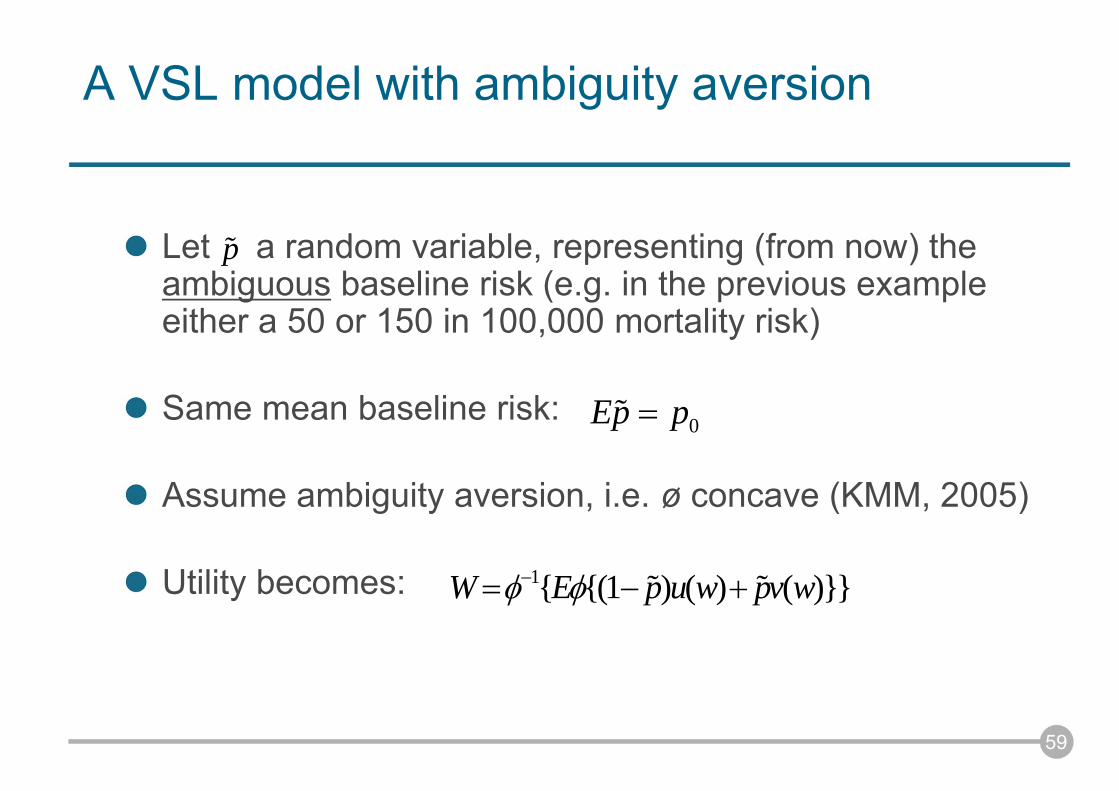
Let a random variable, representing (from now) the ambiguous baseline risk (e.g. in the previous exampleeither a 50 or 150 in 100,000 mortality risk)
Same mean baseline risk:
Assume ambiguity aversion, i.e. ø concave (KMM, 2005)
Utility becomes:
0Ep p
p
1{ {(1 ) ( ) ( )}}W E p u w pv w
60
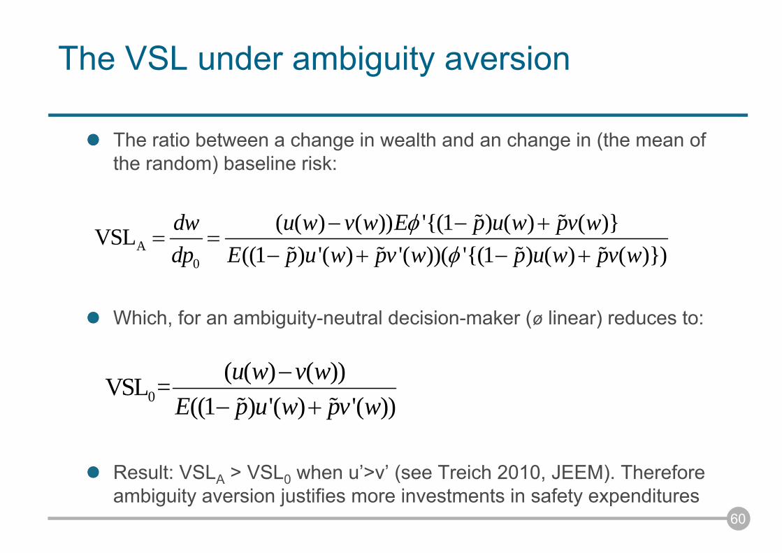
The VSL under ambiguity aversion
The ratio between a change in wealth and an change in (the mean of the random) baseline risk:
Which, for an ambiguity-neutral decision-maker (ø linear) reduces to:
Result: VSLA > VSL0 when u’>v’ (see Treich 2010, JEEM). Thereforeambiguity aversion justifies more investments in safety expenditures
A0
'{(1 ) ( ) ( )}'{(1 ) ( ) ( )}
( ( ) ( ))VSL((1 ) '( ) '( ))( )
dw u w v wdp E
E p u w pv wp u w pvp w pv w wu
0( ( ) ( ))VSL =
((1 ) '( ) '( ))u w v w
E p u w pv w
61
Difficulties with the ambiguity approach
Portfolio of ambiguity (aversion) models – which one to choose?
Few empirical evidence based on market data – can we test these models? what is a « proxy » for ambiguity? how to estimate ambiguity aversion?
Ambiguity aversion theories introduce new anomalies, especially for sequential decision-making (e.g., Al-Najjar and Weinstein 2009, EP):
- Time-inconsistency
- Nonbayesian updating
- Negative value of information
62
Time-inconsistency: An intuition
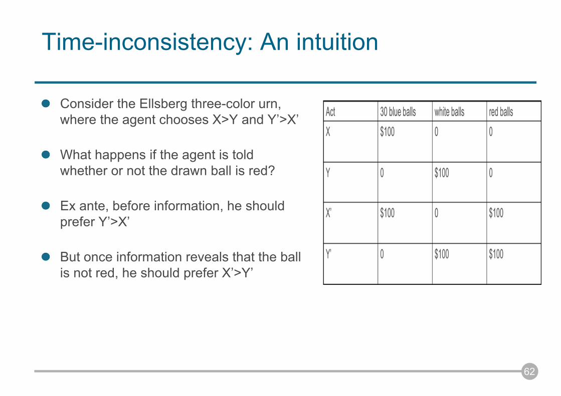
Consider the Ellsberg three-color urn, where the agent chooses X>Y and Y’>X’
What happens if the agent is toldwhether or not the drawn ball is red?
Ex ante, before information, he shouldprefer Y’>X’
But once information reveals that the ballis not red, he should prefer X’>Y’
63
Reconciling the inconsistency?
Sophistication (Siniscalchi 2006), but information aversion
Distorting the updating rule (Hanany and Klibanoff 2007, 2009), but not bayesian updating
« Dynamic consistent beliefs must be bayesian » (Epstein & Le Breton 1993)
Restricting information structures (Sarin & Wakker 1998, Epstein & Schneider 2003, Maccheroni et al. 2006), but one should not « choose » the economic environment sothat it is not problematic for the theory
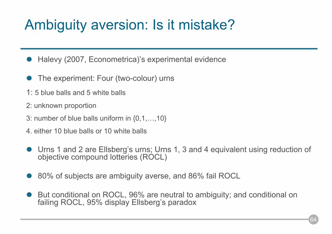
Ambiguity aversion: Is it mistake?
Halevy (2007, Econometrica)’s experimental evidence
The experiment: Four (two-colour) urns
1: 5 blue balls and 5 white balls
2: unknown proportion
3: number of blue balls uniform in {0,1,…,10}
4. either 10 blue balls or 10 white balls
Urns 1 and 2 are Ellsberg’s urns; Urns 1, 3 and 4 equivalent using reduction of objective compound lotteries (ROCL)
80% of subjects are ambiguity averse, and 86% fail ROCL
But conditional on ROCL, 96% are neutral to ambiguity; and conditional on failing ROCL, 95% display Ellsberg’s paradox
64
65
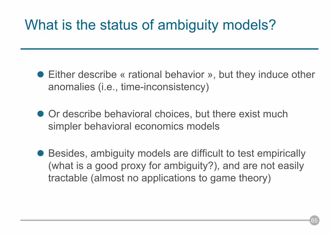
What is the status of ambiguity models?
Either describe « rational behavior », but they induce otheranomalies (i.e., time-inconsistency)
Or describe behavioral choices, but there exist muchsimpler behavioral economics models
Besides, ambiguity models are difficult to test empirically(what is a good proxy for ambiguity?), and are not easilytractable (almost no applications to game theory)
66
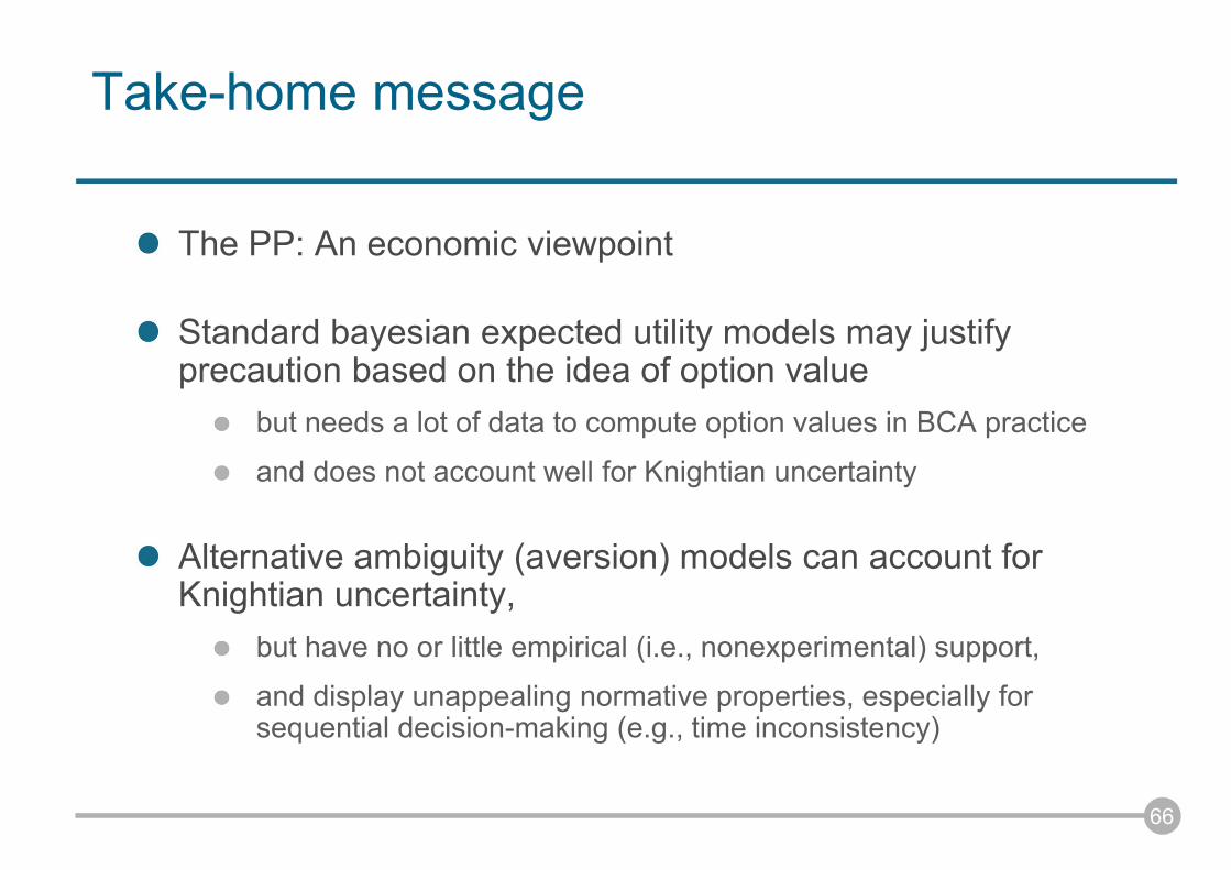
Take-home message
The PP: An economic viewpoint
Standard bayesian expected utility models may justifyprecaution based on the idea of option value
but needs a lot of data to compute option values in BCA practice
and does not account well for Knightian uncertainty
Alternative ambiguity (aversion) models can account for Knightian uncertainty,
but have no or little empirical (i.e., nonexperimental) support,
and display unappealing normative properties, especially for sequential decision-making (e.g., time inconsistency)
67
Some references
« The effect of ambiguity aversion on insurance and self-protection » 2012, Economic Journal , forthcoming. (with David Alary and Christian Gollier)
« Option value and precaution » 2012, in Encyclopedia of Energy, Natural Resources and Environmental Economics edited by J. Shogren, forthcoming. (with Christian Gollier)
« The value of a statistical life under ambiguity aversion », 2010, Journal of Environmental Economics and Management, 59, 15-26.
« Precautionary Principle », 2008, The New Palgrave Dictionary of Economics, Second Edition (withChristian Gollier)
« Uncertainty, learning and ambiguity in climate policy: Some classical results and new directions », 2008, Climatic Change, 89, 7-21. (with Andreas Lange)
« Risk-aversion, intergenerational equity and climate change », 2004, Environmental and Resource Economics, 28, 195-207. (with Minh Ha-duong).
« Decision-making under scientific uncertainty: The economics of the Precautionary Principle», 2003, Journal of Risk and Uncertainty, 27, 77-103. (with Christian Gollier).
« Scientific progress and irreversibility: An economic interpretation of the Precautionary Principle », 2000, Journal of Public Economics, 75, 229-53. (with Christian Gollier and Bruno Jullien).