Independent Component Analysis� A Tutorial

Aapo Hyv�rinen and Erkki Oja

Helsinki University of Technology

Laboratory of Computer and Information Science

P�O� Box ����� FIN������ Espoo� Finland

aapo�hyvarinen�hut�fi� erkki�oja�hut�fi

http���www�cis�hut�fi�projects�ica�

A version of this paper will appear in Neural Networks

with the title Independent Component Analysis Algorithms and Applications�

April ����

� Motivation

Imagine that you are in a room where two people are speaking simultaneously� You have two microphones�which you hold in di�erent locations� The microphones give you two recorded time signals� which we coulddenote by x��t� and x��t�� with x� and x� the amplitudes� and t the time index� Each of these recordedsignals is a weighted sum of the speech signals emitted by the two speakers� which we denote by s��t� ands��t�� We could express this as a linear equation�

x��t� � a��s� � a��s� ���

x��t� � a��s� � a��s� ���

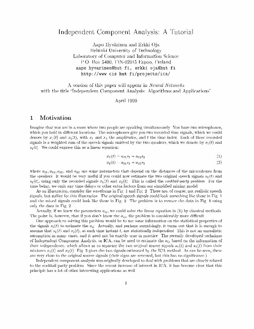
where a��� a��� a��� and a�� are some parameters that depend on the distances of the microphones fromthe speakers� It would be very useful if you could now estimate the two original speech signals s��t� ands��t�� using only the recorded signals x��t� and x��t�� This is called the cocktail�party problem� For thetime being� we omit any time delays or other extra factors from our simpli�ed mixing model�As an illustration� consider the waveforms in Fig� � and Fig� �� These are� of course� not realistic speech

signals� but suce for this illustration� The original speech signals could look something like those in Fig� �and the mixed signals could look like those in Fig� �� The problem is to recover the data in Fig� � usingonly the data in Fig� ��Actually� if we knew the parameters aij � we could solve the linear equation in ��� by classical methods�

The point is� however� that if you dont know the aij � the problem is considerably more dicult�One approach to solving this problem would be to use some information on the statistical properties of

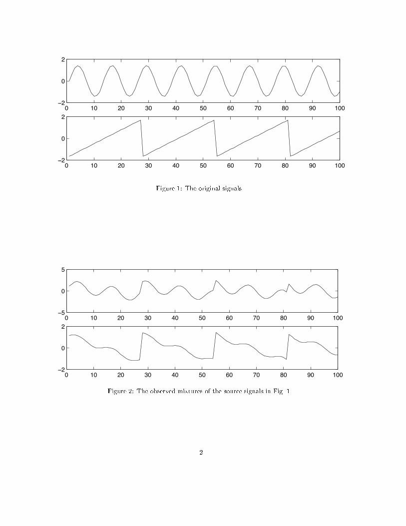
the signals si�t� to estimate the aii� Actually� and perhaps surprisingly� it turns out that it is enough toassume that s��t� and s��t�� at each time instant t� are statistically independent� This is not an unrealisticassumption in many cases� and it need not be exactly true in practice� The recently developed techniqueof Independent Component Analysis� or ICA� can be used to estimate the aij based on the information oftheir independence� which allows us to separate the two original source signals s��t� and s��t� from theirmixtures x��t� and x��t�� Fig� � gives the two signals estimated by the ICA method� As can be seen� theseare very close to the original source signals �their signs are reversed� but this has no signi�cance��Independent component analysis was originally developed to deal with problems that are closely related

to the cocktail�party problem� Since the recent increase of interest in ICA� it has become clear that thisprinciple has a lot of other interesting applications as well�

�

0 10 20 30 40 50 60 70 80 90 100−2

0

2

0 10 20 30 40 50 60 70 80 90 100−2

0

2

Figure �� The original signals�

0 10 20 30 40 50 60 70 80 90 100−5

0

5

0 10 20 30 40 50 60 70 80 90 100−2

0

2

Figure �� The observed mixtures of the source signals in Fig� ��

�

0 10 20 30 40 50 60 70 80 90 100−2

0

2

0 10 20 30 40 50 60 70 80 90 100−2

0

2

Figure �� The estimates of the original source signals� estimated using only the observed signals in Fig� ��The original signals were very accurately estimated� up to multiplicative signs�

Consider� for example� electrical recordings of brain activity as given by an electroencephalogram �EEG��The EEG data consists of recordings of electrical potentials in many di�erent locations on the scalp�These potentials are presumably generated by mixing some underlying components of brain activity� Thissituation is quite similar to the cocktail�party problem� we would like to �nd the original components ofbrain activity� but we can only observe mixtures of the components� ICA can reveal interesting informationon brain activity by giving access to its independent components�Another� very di�erent application of ICA is on feature extraction� A fundamental problem in digital

signal processing is to �nd suitable representations for image� audio or other kind of data for tasks likecompression and denoising� Data representations are often based on �discrete� linear transformations�Standard linear transformations widely used in image processing are the Fourier� Haar� cosine transformsetc� Each of them has its own favorable properties ����It would be most useful to estimate the linear transformation from the data itself� in which case the

transform could be ideally adapted to the kind of data that is being processed� Figure � shows the basisfunctions obtained by ICA from patches of natural images� Each image window in the set of training imageswould be a superposition of these windows so that the coecient in the superposition are independent�Feature extraction by ICA will be explained in more detail later on�All of the applications described above can actually be formulated in a uni�ed mathematical framework�

that of ICA� This is a very general�purpose method of signal processing and data analysis�In this review� we cover the de�nition and underlying principles of ICA in Sections � and �� Then�

starting from Section �� the ICA problem is solved on the basis of minimizing or maximizing certainconrast functions� this transforms the ICA problem to a numerical optimization problem� Many contrastfunctions are given and the relations between them are clari�ed� Section � covers a useful preprocessing thatgreatly helps solving the ICA problem� and Section � reviews one of the most ecient practical learningrules for solving the problem� the FastICA algorithm� Then� in Section �� typical applications of ICA arecovered� removing artefacts from brain signal recordings� �nding hidden factors in �nancial time series�and reducing noise in natural images� Section � concludes the text�

�

Figure �� Basis functions in ICA of natural images� The input window size was ��� �� pixels� These basisfunctions can be considered as the independent features of images�

�

� Independent Component Analysis

��� De�nition of ICA

To rigorously de�ne ICA ��� ��� we can use a statistical �latent variables� model� Assume that we observen linear mixtures x�� ���� xn of n independent components

xj � aj�s� � aj�s� � ���� ajnsn� for all j� ���

We have now dropped the time index t� in the ICA model� we assume that each mixture xj as wellas each independent component sk is a random variable� instead of a proper time signal� The observedvalues xj�t�� e�g�� the microphone signals in the cocktail party problem� are then a sample of this randomvariable� Without loss of generality� we can assume that both the mixture variables and the independentcomponents have zero mean� If this is not true� then the observable variables xi can always be centered bysubtracting the sample mean� which makes the model zero�mean�It is convenient to use vector�matrix notation instead of the sums like in the previous equation� Let us

denote by x the random vector whose elements are the mixtures x�� ���� xn� and likewise by s the randomvector with elements s�� ���� sn� Let us denote by A the matrix with elements aij � Generally� bold lowercase letters indicate vectors and bold upper�case letters denote matrices� All vectors are understood ascolumn vectors� thus xT � or the transpose of x� is a row vector� Using this vector�matrix notation� theabove mixing model is written as

x � As� ���

Sometimes we need the columns of matrix A� denoting them by aj the model can also be written as

x �nXi��

aisi� ���

The statistical model in Eq� � is called independent component analysis� or ICA model� The ICA modelis a generative model� which means that it describes how the observed data are generated by a process ofmixing the components si� The independent components are latent variables� meaning that they cannotbe directly observed� Also the mixing matrix is assumed to be unknown� All we observe is the randomvector x� and we must estimate both A and s using it� This must be done under as general assumptionsas possible�The starting point for ICA is the very simple assumption that the components si are statistically

independent� Statistical independence will be rigorously de�ned in Section �� It will be seen below that wemust also assume that the independent component must have nongaussian distributions� However� in thebasic model we do not assume these distributions known �if they are known� the problem is considerablysimpli�ed�� For simplicity� we are also assuming that the unknown mixing matrix is square� but thisassumption can be sometimes relaxed� as explained in Section ���� Then� after estimating the matrix A�we can compute its inverse� sayW� and obtain the independent component simply by�

s �Wx� ���

ICA is very closely related to the method called blind source separation �BSS� or blind signal separa�tion� A �source� means here an original signal� i�e� independent component� like the speaker in a cocktailparty problem� �Blind� means that we no very little� if anything� on the mixing matrix� and make littleassumptions on the source signals� ICA is one method� perhaps the most widely used� for performing blindsource separation�In many applications� it would be more realistic to assume that there is some noise in the measurements

�see e�g� ��� ����� which would mean adding a noise term in the model� For simplicity� we omit any noiseterms� since the estimation of the noise�free model is dicult enough in itself� and seems to be sucientfor many applications�

�

��� Ambiguities of ICA

In the ICA model in Eq� ���� it is easy to see that the following ambiguities will hold�

�� We cannot determine the variances �energies� of the independent components�

The reason is that� both s and A being unknown� any scalar multiplier in one of the sources si couldalways be cancelled by dividing the corresponding column ai of A by the same scalar� see eq� ���� As aconsequence� we may quite as well �x the magnitudes of the independent components� as they are randomvariables� the most natural way to do this is to assume that each has unit variance� Efs�i g � �� Then thematrix A will be adapted in the ICA solution methods to take into account this restriction� Note thatthis still leaves the ambiguity of the sign� we could multiply the an independent component by �� withouta�ecting the model� This ambiguity is� fortunately� insigni�cant in most applications�

�� We cannot determine the order of the independent components�

The reason is that� again both s and A being unknown� we can freely change the order of the terms inthe sum in ���� and call any of the independent components the �rst one� Formally� a permutation matrixP and its inverse can be substituted in the model to give x � AP��Ps� The elements of Ps are the originalindependent variables sj � but in another order� The matrix AP

�� is just a new unknown mixing matrix�to be solved by the ICA algorithms�

��� Illustration of ICA

To illustrate the ICA model in statistical terms� consider two independent components that have thefollowing uniform distributions�

p�si� �

��

�p�if jsij �

p�

� otherwise���

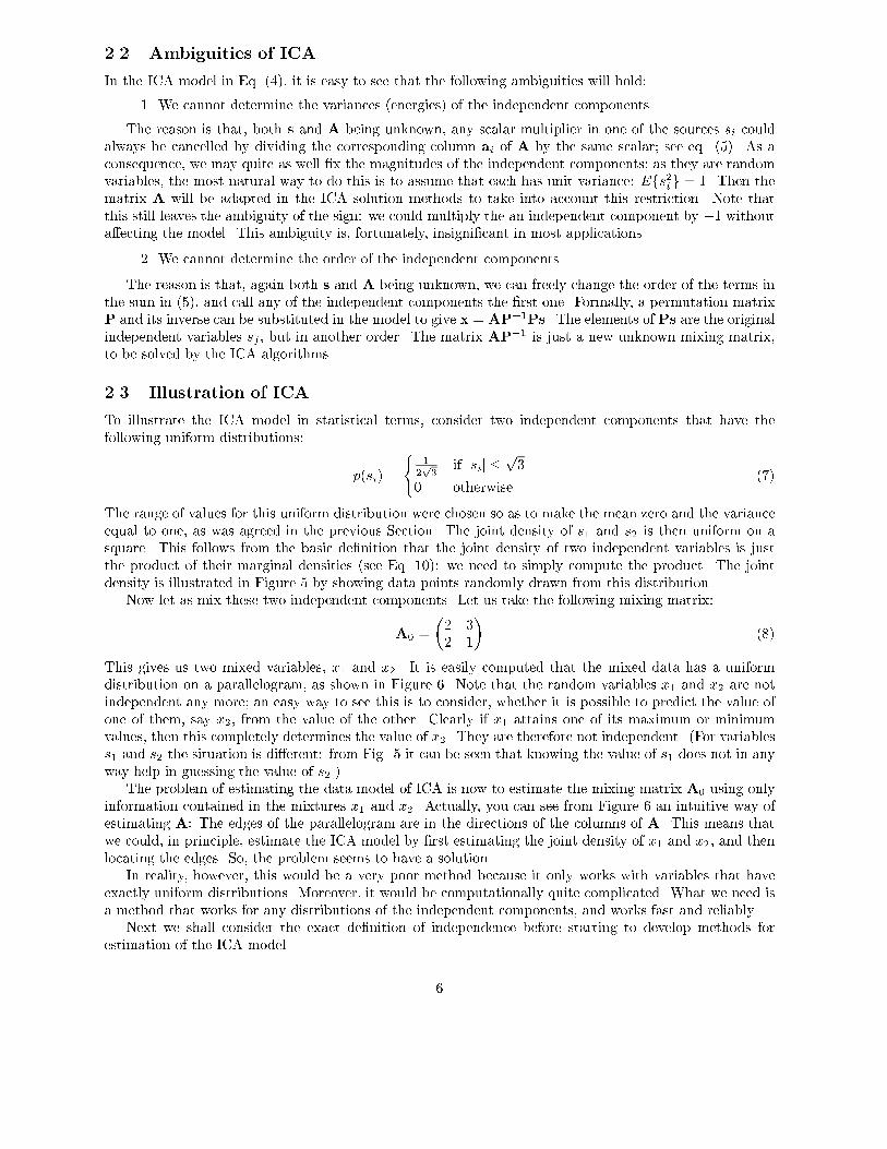
The range of values for this uniform distribution were chosen so as to make the mean zero and the varianceequal to one� as was agreed in the previous Section� The joint density of s� and s� is then uniform on asquare� This follows from the basic de�nition that the joint density of two independent variables is justthe product of their marginal densities �see Eq� ���� we need to simply compute the product� The jointdensity is illustrated in Figure � by showing data points randomly drawn from this distribution�Now let as mix these two independent components� Let us take the following mixing matrix�

A� �

�� �� �

����

This gives us two mixed variables� x� and x�� It is easily computed that the mixed data has a uniformdistribution on a parallelogram� as shown in Figure �� Note that the random variables x� and x� are notindependent any more� an easy way to see this is to consider� whether it is possible to predict the value ofone of them� say x�� from the value of the other� Clearly if x� attains one of its maximum or minimumvalues� then this completely determines the value of x�� They are therefore not independent� �For variabless� and s� the situation is di�erent� from Fig� � it can be seen that knowing the value of s� does not in anyway help in guessing the value of s���The problem of estimating the data model of ICA is now to estimate the mixing matrix A� using only

information contained in the mixtures x� and x�� Actually� you can see from Figure � an intuitive way ofestimating A� The edges of the parallelogram are in the directions of the columns of A� This means thatwe could� in principle� estimate the ICA model by �rst estimating the joint density of x� and x�� and thenlocating the edges� So� the problem seems to have a solution�In reality� however� this would be a very poor method because it only works with variables that have

exactly uniform distributions� Moreover� it would be computationally quite complicated� What we need isa method that works for any distributions of the independent components� and works fast and reliably�Next we shall consider the exact de�nition of independence before starting to develop methods for

estimation of the ICA model�

�

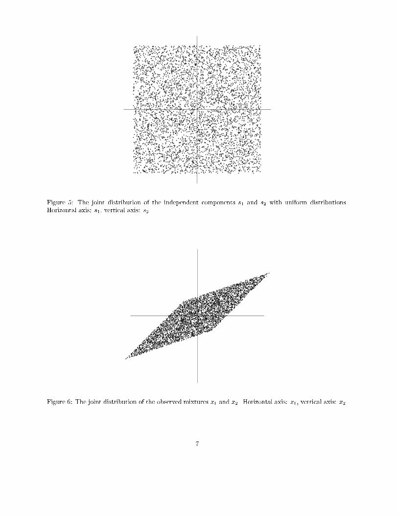
Figure �� The joint distribution of the independent components s� and s� with uniform distributions�Horizontal axis� s�� vertical axis� s��

Figure �� The joint distribution of the observed mixtures x� and x�� Horizontal axis� x�� vertical axis� x��

�

� What is independence�

��� De�nition and fundamental properties

To de�ne the concept of independence� consider two scalar�valued random variables y� and y�� Basically�the variables y� and y� are said to be independent if information on the value of y� does not give anyinformation on the value of y�� and vice versa� Above� we noted that this is the case with the variabless�� s� but not with the mixture variables x�� x��Technically� independence can be de�ned by the probability densities� Let us denote by p�y�� y�� the

joint probability density function �pdf� of y� and y�� Let us further denote by p��y�� the marginal pdf ofy�� i�e� the pdf of y� when it is considered alone�

p��y�� �

Zp�y�� y��dy�� ���

and similarly for y�� Then we de�ne that y� and y� are independent if and only if the joint pdf is factorizablein the following way�

p�y�� y�� � p��y��p��y��� ����

This de�nition extends naturally for any number n of random variables� in which case the joint densitymust be a product of n terms�The de�nition can be used to derive a most important property of independent random variables� Given

two functions� h� and h�� we always have

Efh��y��h��y��g � Efh��y��gEfh��y��g� ����

This can be proven as follows�

Efh��y��h��y��g �

Z Zh��y��h��y��p�y�� y��dy�dy�

�

Z Zh��y��p��y��h��y��p��y��dy�dy� �

Zh��y��p��y��dy�

Zh��y��p��y��dy�

� Efh��y��gEfh��y��g� ����

��� Uncorrelated variables are only partly independent

A weaker form of independence is uncorrelatedness� Two random variables y� and y� are said to beuncorrelated� if their covariance is zero�

Efy�y�g �Efy�gEfy�g � � ����

If the variables are independent� they are uncorrelated� which follows directly from Eq� ����� taking h��y�� �y� and h��y�� � y��On the other hand� uncorrelatedness does not imply independence� For example� assume that �y�� y��

are discrete valued and follow such a distribution that the pair are with probability �� equal to any of thefollowing values� ��� ��� ������� ��� ��� ���� ��� Then y� and y� are uncorrelated� as can be simply calculated�On the other hand�

Efy��y��g � � �� �� � Efy��gEfy��g� ����

so the condition in Eq� ���� is violated� and the variables cannot be independent�Since independence implies uncorrelatedness� many ICA methods constrain the estimation procedure

so that it always gives uncorrelated estimates of the independent components� This reduces the number offree parameters� and simpli�es the problem�

�

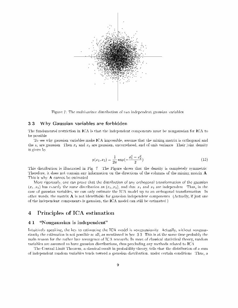
Figure �� The multivariate distribution of two independent gaussian variables�

��� Why Gaussian variables are forbidden

The fundamental restriction in ICA is that the independent components must be nongaussian for ICA tobe possible�To see why gaussian variables make ICA impossible� assume that the mixing matrix is orthogonal and

the si are gaussian� Then x� and x� are gaussian� uncorrelated� and of unit variance� Their joint densityis given by

p�x�� x�� ��

��exp��x�� � x��

�� ����

This distribution is illustrated in Fig� �� The Figure shows that the density is completely symmetric�Therefore� it does not contain any information on the directions of the columns of the mixing matrix A�This is why A cannot be estimated�More rigorously� one can prove that the distribution of any orthogonal transformation of the gaussian

�x�� x�� has exactly the same distribution as �x�� x��� and that x� and x� are independent� Thus� in thecase of gaussian variables� we can only estimate the ICA model up to an orthogonal transformation� Inother words� the matrix A is not identi�able for gaussian independent components� �Actually� if just oneof the independent components is gaussian� the ICA model can still be estimated��

� Principles of ICA estimation

��� �Nongaussian is independent�

Intuitively speaking� the key to estimating the ICA model is nongaussianity� Actually� without nongaus�sianity the estimation is not possible at all� as mentioned in Sec� ���� This is at the same time probably themain reason for the rather late resurgence of ICA research� In most of classical statistical theory� randomvariables are assumed to have gaussian distributions� thus precluding any methods related to ICA�The Central Limit Theorem� a classical result in probability theory� tells that the distribution of a sum

of independent random variables tends toward a gaussian distribution� under certain conditions� Thus� a

�

sum of two independent random variables usually has a distribution that is closer to gaussian than any ofthe two original random variables�Let us now assume that the data vector x is distributed according to the ICA data model in Eq� ��

i�e� it is a mixture of independent components� For simplicity� let us assume in this section that all theindependent components have identical distributions� To estimate one of the independent components� weconsider a linear combination of the xi �see eq� ��� let us denote this by y � wTx �

Pi wixi� where w is

a vector to be determined� If w were one of the rows of the inverse of A� this linear combination wouldactually equal one of the independent components� The question is now� How could we use the CentralLimit Theorem to determine w so that it would equal one of the rows of the inverse of A� In practice�we cannot determine such a w exactly� because we have no knowledge of matrix A� but we can �nd anestimator that gives a good approximation�To see how this leads to the basic principle of ICA estimation� let us make a change of variables� de�ning

z � ATw� Then we have y � wTx � wTAs � zT s� y is thus a linear combination of si� with weights givenby zi� Since a sum of even two independent random variables is more gaussian than the original variables�zT s is more gaussian than any of the si and becomes least gaussian when it in fact equals one of the si�In this case� obviously only one of the elements zi of z is nonzero� �Note that the si were here assumed tohave identical distributions��Therefore� we could take as w a vector that maximizes the nongaussianity of wTx� Such a vector

would necessarily correspond �in the transformed coordinate system� to a z which has only one nonzerocomponent� This means that wTx � zT s equals one of the independent components�Maximizing the nongaussianity of wTx thus gives us one of the independent components� In fact� the

optimization landscape for nongaussianity in the n�dimensional space of vectorsw has �n local maxima� twofor each independent component� corresponding to si and �si �recall that the independent components canbe estimated only up to a multiplicative sign�� To �nd several independent components� we need to �nd allthese local maxima� This is not dicult� because the di�erent independent components are uncorrelated�We can always constrain the search to the space that gives estimates uncorrelated with the previous ones�This corresponds to orthogonalization in a suitably transformed �i�e� whitened� space�Our approach here is rather heuristic� but it will be seen in the next section and Sec� ��� that it has a

perfectly rigorous justi�cation�

��� Measures of nongaussianity

To use nongaussianity in ICA estimation� we must have a quantitative measure of nongaussianity of arandom variable� say y� To simplify things� let us assume that y is centered �zero�mean� and has varianceequal to one� Actually� one of the functions of preprocessing in ICA algorithms� to be covered in Section ��is to make this simpli�cation possible�

����� Kurtosis

The classical measure of nongaussianity is kurtosis or the fourth�order cumulant� The kurtosis of y isclassically de�ned by

kurt�y� � Efy�g � ��Efy�g�� ����

Actually� since we assumed that y is of unit variance� the right�hand side simpli�es to Efy�g � �� Thisshows that kurtosis is simply a normalized version of the fourth moment Efy�g� For a gaussian y� thefourth moment equals ��Efy�g��� Thus� kurtosis is zero for a gaussian random variable� For most �but notquite all� nongaussian random variables� kurtosis is nonzero�Kurtosis can be both positive or negative� Random variables that have a negative kurtosis are called

subgaussian� and those with positive kurtosis are called supergaussian� In statistical literature� the cor�responding expressions platykurtic and leptokurtic are also used� Supergaussian random variables havetypically a �spiky� pdf with heavy tails� i�e� the pdf is relatively large at zero and at large values of the

��

−4 −3 −2 −1 0 1 2 3 40

0.1

0.2

0.3

0.4

0.5

0.6

0.7

0.8

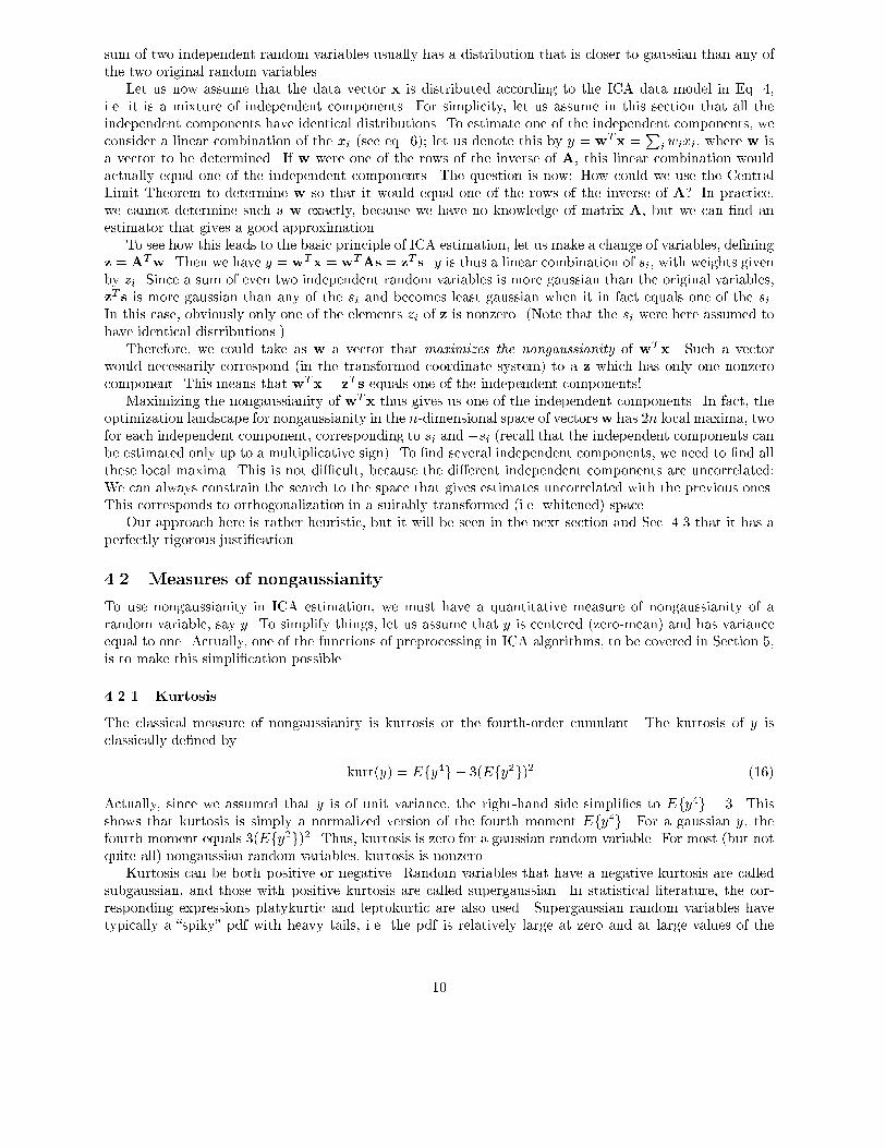
Figure �� The density function of the Laplace distribution� which is a typical supergaussian distribution�For comparison� the gaussian density is given by a dashed line� Both densities are normalized ot unitvariance�

variable� while being small for intermediate values� A typical example is the Laplace distribution� whosepdf �normalized to unit variance� is given by

p�y� ��p�exp�

p�jyj� ����

This pdf is illustrated in Fig� �� Subgaussian random variables� on the other hand� have typically a ��at�pdf� which is rather constant near zero� and very small for larger values of the variable� A typical exampleis the uniform distibution in eq� ����Typically nongaussianity is measured by the absolute value of kurtosis� The square of kurtosis can

also be used� These are zero for a gaussian variable� and greater than zero for most nongaussian randomvariables� There are nongaussian random variables that have zero kurtosis� but they can be considered asvery rare�Kurtosis� or rather its absolute value� has been widely used as a measure of nongaussianity in ICA and

related �elds� The main reason is its simplicity� both computational and theoretical� Computationally�kurtosis can be estimated simply by using the fourth moment of the sample data� Theoretical analysis issimpli�ed because of the following linearity property� If x� and x� are two independent random variables�it holds

kurt�x� � x�� � kurt�x�� � kurt�x�� ����

and

kurt��x�� � �� kurt�x�� ����

where � is a scalar� These properties can be easily proven using the de�nition�To illustrate in a simple example what the optimization landscape for kurtosis looks like� and how

independent components could be found by kurtosis minimization or maximization� let us look at a��dimensional model x � As� Assume that the independent components s�� s� have kurtosis valueskurt�s��� kurt�s��� respectively� both di�erent from zero� Remember that we assumed that they haveunit variances� We seek for one of the independent components as y � wTx�Let us again make the transformation z � ATw� Then we have y � wTx � wTAs � zT s � z�s��z�s��

Now� based on the additive property of kurtosis� we have kurt�y� � kurt�z�s��� kurt�z�s�� � z�� kurt�s���

��

z�� kurt�s��� On the other hand� we made the constraint that the variance of y is equal to �� based on thesame assumption concerning s�� s�� This implies a constraint on z� Efy�g � z�� � z�� � �� Geometrically�this means that vector z is constrained to the unit circle on the ��dimensional plane� The optimizationproblem is now� what are the maxima of the function j kurt�y�j � jz�� kurt�s�� � z�� kurt�s��j on the unitcircle� For simplicity� you may consider that the kurtosis are of the same sign� in which case it absolutevalue operators can be omitted� The graph of this function is the �optimization landscape� for the problem�It is not hard to show �� that the maxima are at the points when exactly one of the elements of vector

z is zero and the other nonzero� because of the unit circle constraint� the nonzero element must be equalto � or ��� But these points are exactly the ones when y equals one of the independent components �si�and the problem has been solved�In practice we would start from some weight vector w� compute the direction in which the kurtosis

of y � wTx is growing most strongly �if kurtosis is positive� or decreasing most strongly �if kurtosis isnegative� based on the available sample x���� ����x�T � of mixture vector x� and use a gradient method orone of their extensions for �nding a new vector w� The example can be generalized to arbitrary dimensions�showing that kurtosis can theoretically be used as an optimization criterion for the ICA problem�However� kurtosis has also some drawbacks in practice� when its value has to be estimated from a

measured sample� The main problem is that kurtosis can be very sensitive to outliers ���� Its value maydepend on only a few observations in the tails of the distribution� which may be erroneous or irrelevantobservations� In other words� kurtosis is not a robust measure of nongaussianity�Thus� other measures of nongaussianity might be better than kurtosis in some situations� Below we

shall consider negentropy whose properties are rather opposite to those of kurtosis� and �nally introduceapproximations of negentropy that more or less combine the good properties of both measures�

����� Negentropy

A second very important measure of nongaussianity is given by negentropy� Negentropy is based on theinformation�theoretic quantity of �di�erential� entropy�Entropy is the basic concept of information theory� The entropy of a random variable can be inter�

preted as the degree of information that the observation of the variable gives� The more �random�� i�e�unpredictable and unstructured the variable is� the larger its entropy� More rigorously� entropy is closelyrelated to the coding length of the random variable� in fact� under some simplifying assumptions� entropyis the coding length of the random variable� For introductions on information theory� see e�g� �� ����Entropy H is de�ned for a discrete random variable Y as

H�Y � � �Xi

P �Y � ai� logP �Y � ai� ����

where the ai are the possible values of Y � This very well�known de�nition can be generalized for continuous�valued random variables and vectors� in which case it is often called di�erential entropy� The di�erentialentropy H of a random vector y with density f�y� is de�ned as �� ����

H�y� � �Z

f�y� log f�y�dy� ����

A fundamental result of information theory is that a gaussian variable has the largest entropy amongall random variables of equal variance� For a proof� see e�g� �� ���� This means that entropy could be usedas a measure of nongaussianity� In fact� this shows that the gaussian distribution is the �most random� orthe least structured of all distributions� Entropy is small for distributions that are clearly concentrated oncertain values� i�e�� when the variable is clearly clustered� or has a pdf that is very �spiky��To obtain a measure of nongaussianity that is zero for a gaussian variable and always nonnegative� one

often uses a slightly modi�ed version of the de�nition of di�erential entropy� called negentropy� NegentropyJ is de�ned as follows

J�y� � H�ygauss��H�y� ����

��

where ygauss is a Gaussian random variable of the same covariance matrix as y� Due to the above�mentionedproperties� negentropy is always non�negative� and it is zero if and only if y has a Gaussian distribution�Negentropy has the additional interesting property that it is invariant for invertible linear transformations �� ����The advantage of using negentropy� or� equivalently� di�erential entropy� as a measure of nongaussianity

is that it is well justi�ed by statistical theory� In fact� negentropy is in some sense the optimal estimator ofnongaussianity� as far as statistical properties are concerned� The problem in using negentropy is� however�that it is computationally very dicult� Estimating negentropy using the de�nition would require anestimate �possibly nonparametric� of the pdf� Therefore� simpler approximations of negentropy are veryuseful� as will be discussed next�

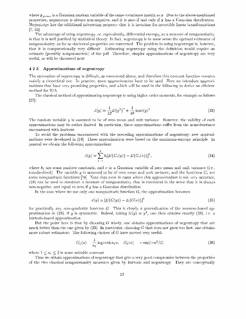
����� Approximations of negentropy

The estimation of negentropy is dicult� as mentioned above� and therefore this contrast function remainsmainly a theoretical one� In practice� some approximation have to be used� Here we introduce approxi�mations that have very promising properties� and which will be used in the following to derive an ecientmethod for ICA�The classical method of approximating negentropy is using higher�order moments� for example as follows

����

J�y� � �

��Efy�g� � �

kurt�y�� ����

The random variable y is assumed to be of zero mean and unit variance� However� the validity of suchapproximations may be rather limited� In particular� these approximations su�er from the nonrobustnessencountered with kurtosis�To avoid the problems encountered with the preceding approximations of negentropy� new approxi�

mations were developed in ���� These approximation were based on the maximum�entropy principle� Ingeneral we obtain the following approximation�

J�y� �pXi��

ki�EfGi�y�g �EfGi���g��� ����

where ki are some positive constants� and � is a Gaussian variable of zero mean and unit variance �i�e��standardized�� The variable y is assumed to be of zero mean and unit variance� and the functions Gi aresome nonquadratic functions ���� Note that even in cases where this approximation is not very accurate����� can be used to construct a measure of nongaussianity that is consistent in the sense that it is alwaysnon�negative� and equal to zero if y has a Gaussian distribution�In the case where we use only one nonquadratic function G� the approximation becomes

J�y� � �EfG�y�g �EfG���g�� ����

for practically any non�quadratic function G� This is clearly a generalization of the moment�based ap�proximation in ����� if y is symmetric� Indeed� taking G�y� � y�� one then obtains exactly ����� i�e� akurtosis�based approximation�But the point here is that by choosing G wisely� one obtains approximations of negentropy that are

much better than the one given by ����� In particular� choosing G that does not grow too fast� one obtainsmore robust estimators� The following choices of G have proved very useful�

G��u� ��

a�log cosha�u� G��u� � � exp��u���� ����

where � � a� � � is some suitable constant�Thus we obtain approximations of negentropy that give a very good compromise between the properties

of the two classical nongaussianity measures given by kurtosis and negentropy� They are conceptually

��

simple� fast to compute� yet have appealing statistical properties� especially robustness� Therefore� we shalluse these contrast functions in our ICA methods� Since kurtosis can be expressed in this same framework�it can still be used by our ICA methods� A practical algorithm based on these contrast function will bepresented in Section ��

��� Minimization of Mutual Information

Another approach for ICA estimation� inspired by information theory� is minimization of mutual informa�tion� We will explain this approach here� and show that it leads to the same principle of �nding mostnongaussian directions as was described above� In particular� this approach gives a rigorous justi�cationfor the heuristic principles used above�

����� Mutual Information

Using the concept of di�erential entropy� we de�ne the mutual information I between m �scalar� randomvariables� yi� i � ����m as follows

I�y�� y�� ���� ym� �

mXi��

H�yi��H�y�� ����

Mutual information is a natural measure of the dependence between random variables� In fact� it isequivalent to the well�known Kullback�Leibler divergence between the joint density f�y� and the productof its marginal densities� a very natural measure for independence� It is always non�negative� and zero ifand only if the variables are statistically independent� Thus� mutual information takes into account thewhole dependence structure of the variables� and not only the covariance� like PCA and related methods�Mutual information can be interpreted by using the interpretation of entropy as code length� The

terms H�yi� give the lengths of codes for the yi when these are coded separately� and H�y� gives the codelength when y is coded as a random vector� i�e� all the components are coded in the same code� Mutualinformation thus shows what code length reduction is obtained by coding the whole vector instead of theseparate components� In general� better codes can be obtained by coding the whole vector� However� if theyi are independent� they give no information on each other� and one could just as well code the variablesseparately without increasing code length�An important property of mutual information ��� �� is that we have for an invertible linear transfor�

mation y �Wx�

I�y�� y�� ���� yn� �Xi

H�yi��H�x� � log j detWj� ����

Now� let us consider what happens if we constrain the yi to be uncorrelated and of unit variance� This meansEfyyT g �WEfxxT gWT � I� which implies det I � � � �detWEfxxT gWT � � �detW��detEfxxT g��detWT ��and this implies that detW must be constant� Moreover� for yi of unit variance� entropy and negentropydi�er only by a constant� and the sign� Thus we obtain�

I�y�� y�� ���� yn� � C �Xi

J�yi�� ����

where C is a constant that does not depend onW� This shows the fundamental relation between negentropyand mutual information�

����� De�ning ICA by Mutual Information

Since mutual information is the natural information�theoretic measure of the independence of random vari�ables� we could use it as the criterion for �nding the ICA transform� In this approach that is an alternativeto the model estimation approach� we de�ne the ICA of a random vector x as an invertible transformation

��

as in ���� where the matrixW is determined so that the mutual information of the transformed componentssi is minimized�It is now obvious from ���� that �nding an invertible transformation W that minimizes the mutual

information is roughly equivalent to �nding directions in which the negentropy is maximized� More precisely�it is roughly equivalent to �nding ��D subspaces such that the projections in those subspaces have maximumnegentropy� Rigorously� speaking� ���� shows that ICA estimation by minimization of mutual information isequivalent to maximizing the sum of nongaussianities of the estimates� when the estimates are constrained tobe uncorrelated� The constraint of uncorrelatedness is in fact not necessary� but simpli�es the computationsconsiderably� as one can then use the simpler form in ���� instead of the more complicated form in �����Thus� we see that the formulation of ICA as minimization of mutual information gives another rigorous

justi�cation of our more heuristically introduced idea of �nding maximally nongaussian directions�

��� Maximum Likelihood Estimation

����� The likelihood

A very popular approach for estimating the ICA model is maximum likelihood estimation� which is closelyconnected to the infomax principle� Here we discuss this approach� and show that it is essentially equivalentto minimization of mutual information�It is possible to formulate directly the likelihood in the noise�free ICA model� which was done in ����

and then estimate the model by a maximum likelihood method� Denoting byW � �w�� ����wn�T the matrix

A��� the log�likelihood takes the form ����

L �

TXt��

nXi��

log fi�wTi x�t�� � T log j detWj ����

where the fi are the density functions of the si �here assumed to be known�� and the x�t�� t � �� ���� Tare the realizations of x� The term log j detWj in the likelihood comes from the classic rule for �linearly�transforming random variables and their densities ���� In general� for any random vector x with densitypx and for any matrixW� the density of y �Wx is given by px�Wx�j detWj�

����� The Infomax Principle

Another related contrast function was derived from a neural network viewpoint in �� ���� This was based onmaximizing the output entropy �or information �ow� of a neural network with non�linear outputs� Assumethat x is the input to the neural network whose outputs are of the form gi�w

Ti x�� where the gi are some

non�linear scalar functions� and the wi are the weight vectors of the neurons� One then wants to maximizethe entropy of the outputs�

L� � H�g��wT� x�� ���� gn�w

Tnx��� ����

If the gi are well chosen� this framework also enables the estimation of the ICA model� Indeed� severalauthors� e�g�� �� ���� proved the surprising result that the principle of network entropy maximization�or �infomax�� is equivalent to maximum likelihood estimation� This equivalence requires that the non�linearities gi used in the neural network are chosen as the cumulative distribution functions correspondingto the densities fi� i�e�� g

�i��� � fi����

����� Connection to mutual information

To see the connection between likelihood and mutual information� consider the expectation of the log�likelihood�

�

TEfLg �

nXi��

Eflog fi�wTi x�g� log j detWj� ����

��

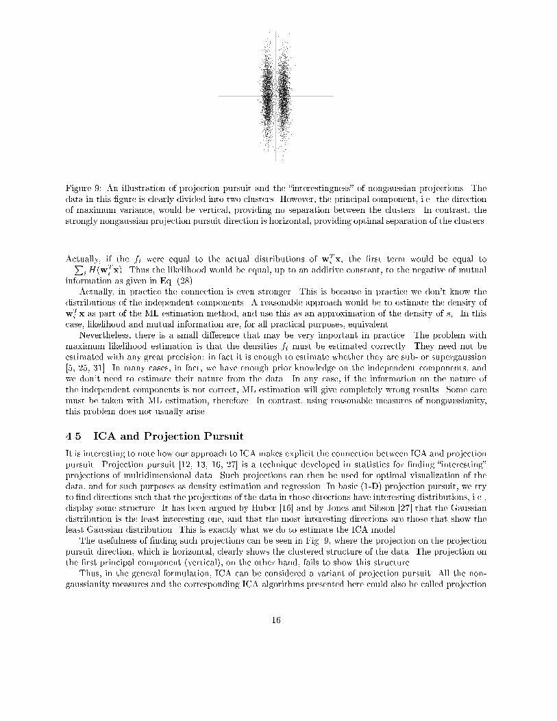
Figure �� An illustration of projection pursuit and the �interestingness� of nongaussian projections� Thedata in this �gure is clearly divided into two clusters� However� the principal component� i�e� the directionof maximum variance� would be vertical� providing no separation between the clusters� In contrast� thestrongly nongaussian projection pursuit direction is horizontal� providing optimal separation of the clusters�

Actually� if the fi were equal to the actual distributions of wTi x� the �rst term would be equal to

�PiH�wTi x�� Thus the likelihood would be equal� up to an additive constant� to the negative of mutual

information as given in Eq� �����Actually� in practice the connection is even stronger� This is because in practice we dont know the

distributions of the independent components� A reasonable approach would be to estimate the density ofwTi x as part of the ML estimation method� and use this as an approximation of the density of si� In this

case� likelihood and mutual information are� for all practical purposes� equivalent�Nevertheless� there is a small di�erence that may be very important in practice� The problem with

maximum likelihood estimation is that the densities fi must be estimated correctly� They need not beestimated with any great precision� in fact it is enough to estimate whether they are sub� or supergaussian �� ��� ���� In many cases� in fact� we have enough prior knowledge on the independent components� andwe dont need to estimate their nature from the data� In any case� if the information on the nature ofthe independent components is not correct� ML estimation will give completely wrong results� Some caremust be taken with ML estimation� therefore� In contrast� using reasonable measures of nongaussianity�this problem does not usually arise�

��� ICA and Projection Pursuit

It is interesting to note how our approach to ICA makes explicit the connection between ICA and projectionpursuit� Projection pursuit ��� ��� ��� ��� is a technique developed in statistics for �nding �interesting�projections of multidimensional data� Such projections can then be used for optimal visualization of thedata� and for such purposes as density estimation and regression� In basic ���D� projection pursuit� we tryto �nd directions such that the projections of the data in those directions have interesting distributions� i�e��display some structure� It has been argued by Huber ��� and by Jones and Sibson ��� that the Gaussiandistribution is the least interesting one� and that the most interesting directions are those that show theleast Gaussian distribution� This is exactly what we do to estimate the ICA model�The usefulness of �nding such projections can be seen in Fig� �� where the projection on the projection

pursuit direction� which is horizontal� clearly shows the clustered structure of the data� The projection onthe �rst principal component �vertical�� on the other hand� fails to show this structure�Thus� in the general formulation� ICA can be considered a variant of projection pursuit� All the non�

gaussianity measures and the corresponding ICA algorithms presented here could also be called projection

��

pursuit �indices� and algorithms� In particular� the projection pursuit allows us to tackle the situationwhere there are less independent components si than original variables xi is� Assuming that those dimen�sions of the space that are not spanned by the independent components are �lled by gaussian noise� wesee that computing the nongaussian projection pursuit directions� we e�ectively estimate the independentcomponents� When all the nongaussian directions have been found� all the independent components havebeen estimated� Such a procedure can be interpreted as a hybrid of projection pursuit and ICA�However� it should be noted that in the formulation of projection pursuit� no data model or assumption

about independent components is made� If the ICA model holds� optimizing the ICA nongaussianitymeasures produce independent components� if the model does not hold� then what we get are the projectionpursuit directions�

� Preprocessing for ICA

In the preceding section� we discussed the statistical principles underlying ICA methods� Practical algo�rithms based on these principles will be discussed in the next section� However� before applying an ICAalgorithm on the data� it is usually very useful to do some preprocessing� In this section� we discuss somepreprocessing techniques that make the problem of ICA estimation simpler and better conditioned�

��� Centering

The most basic and necessary preprocessing is to center x� i�e� subtract its mean vector m � Efxg soas to make x a zero�mean variable� This implies that s is zero�mean as well� as can be seen by takingexpectations on both sides of Eq� ����This preprocessing is made solely to simplify the ICA algorithms� It does not mean that the mean

could not be estimated� After estimating the mixing matrix A with centered data� we can complete theestimation by adding the mean vector of s back to the centered estimates of s� The mean vector of s isgiven by A��m� where m is the mean that was subtracted in the preprocessing�

��� Whitening

Another useful preprocessing strategy in ICA is to �rst whiten the observed variables� This means thatbefore the application of the ICA algorithm �and after centering�� we transform the observed vector xlinearly so that we obtain a new vector x which is white� i�e� its components are uncorrelated and theirvariances equal unity� In other words� the covariance matrix of x equals the identity matrix�

Ef x xT g � I� ����

The whitening transformation is always possible� One popular method for whitening is to use the eigen�value decomposition �EVD� of the covariance matrix EfxxT g � EDET � where E is the orthogonal matrixof eigenvectors of EfxxT g and D is the diagonal matrix of its eigenvalues� D � diag�d�� ���� dn�� Note thatEfxxT g can be estimated in a standard way from the available sample x���� ����x�T �� Whitening can nowbe done by

x � ED����ETx ����

where the matrixD����is computed by a simple component�wise operation asD���� � diag�d����� � ���� d����n ��

It is easy to check that now Ef x xT g � I�Whitening transforms the mixing matrix into a new one� A� We have from ��� and �����

x � ED����ETAs � As ����

The utility of whitening resides in the fact that the new mixing matrix A is orthogonal� This can be seenfrom

Ef x xT g � AEfssT g AT � A AT � I� ����

��

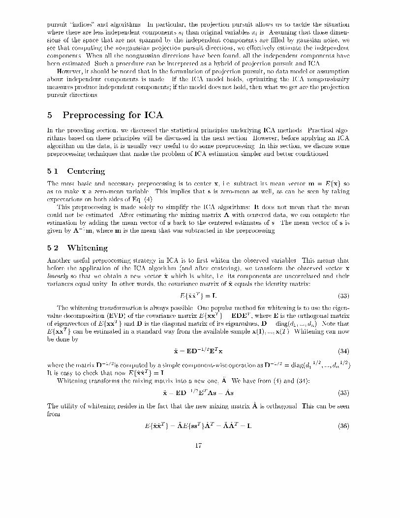
Figure ��� The joint distribution of the whitened mixtures�

Here we see that whitening reduces the number of parameters to be estimated� Instead of having toestimate the n� parameters that are the elements of the original matrix A� we only need to estimatethe new� orthogonal mixing matrix A� An orthogonal matrix contains n�n � ���� degrees of freedom�For example� in two dimensions� an orthogonal transformation is determined by a single angle parameter�In larger dimensions� an orthogonal matrix contains only about half of the number of parameters of anarbitrary matrix� Thus one can say that whitening solves half of the problem of ICA� Because whitening isa very simple and standard procedure� much simpler than any ICA algorithms� it is a good idea to reducethe complexity of the problem this way�It may also be quite useful to reduce the dimension of the data at the same time as we do the whitening�

Then we look at the eigenvalues dj of EfxxT g and discard those that are too small� as is often done in thestatistical technique of principal component analysis� This has often the e�ect of reducing noise� Moreover�dimension reduction prevents overlearning� which can sometimes be observed in ICA ����A graphical illustration of the e�ect of whitening can be seen in Figure ��� in which the data in Figure �

has been whitened� The square de�ning the distribution is now clearly a rotated version of the originalsquare in Figure �� All that is left is the estimation of a single angle that gives the rotation�In the rest of this tutorial� we assume that the data has been preprocessed by centering and whitening�

For simplicity of notation� we denote the preprocessed data just by x� and the transformed mixing matrixby A� omitting the tildes�

��� Further preprocessing

The success of ICA for a given data set may depende crucially on performing some application�dependentpreprocessing steps� For example� if the data consists of time�signals� some band�pass �ltering may be veryuseful� Note that if we �lter linearly the observed signals xi�t� to obtain new signals� say x

�i �t�� the ICA

model still holds for x�i �t�� with the same mixing matrix�This can be seen as follows� Denote byX the matrix that contains the observations x���� ����x�T � as its columns�

and similarly for S� Then the ICA model can be expressed as�

X � AS ����

��

Now� time ltering of X corresponds to multiplying X from the right by a matrix� let us call it M� This gives

X� � XM � ASM � AS�� ���

which shows that the ICA model remains still valid�

� The FastICA Algorithm

In the preceding sections� we introduced di�erent measures of nongaussianity� i�e� objective functions forICA estimation� In practice� one also needs an algorithm for maximizing the contrast function� for examplethe one in ����� In this section� we introduce a very ecient method of maximization suited for this task�It is here assumed that the data is preprocessed by centering and whitening as discussed in the precedingsection�

�� FastICA for one unit

To begin with� we shall show the one�unit version of FastICA� By a �unit� we refer to a computationalunit� eventually an arti�cial neuron� having a weight vector w that the neuron is able to update by alearning rule� The FastICA learning rule �nds a direction� i�e� a unit vector w such that the projectionwTx maximizes nongaussianity� Nongaussianity is here measured by the approximation of negentropyJ�wTx� given in ����� Recall that the variance of wTx must here be constrained to unity� for whiteneddata this is equivalent to constraining the norm of w to be unity�The FastICA is based on a �xed�point iteration scheme for �nding a maximum of the nongaussianity of

wTx� as measured in ����� see ��� ���� It can be also derived as an approximative Newton iteration ����Denote by g the derivative of the nonquadratic function G used in ����� for example the derivatives of thefunctions in ���� are�

g��u� � tanh�a�u�� ����

g��u� � u exp��u����

where � � a� � � is some suitable constant� often taken as a� � �� The basic form of the FastICA algorithmis as follows�

�� Choose an initial �e�g� random� weight vector w�

�� Let w� � Efxg�wTx�g �Efg��wTx�gw�� Let w � w��kw�k�� If not converged� go back to ��

Note that convergence means that the old and new values of w point in the same direction� i�e� theirdot�product is �almost� equal to �� It is not necessary that the vector converges to a single point� since wand �w de�ne the same direction� This is again because the independent components can be de�ned onlyup to a multiplicative sign� Note also that it is here assumed that the data is prewhitened�

The derivation of FastICA is as follows� First note that the maxima of the approximation of the negentropy ofwTx are obtained at certain optima of EfG�wT

x�g� According to the Kuhn�Tucker conditions ��� � the optima ofEfG�wT

x�g under the constraint Ef�wTx��g � kwk� � � are obtained at points where

Efxg�wTx�g � �w � � ����

Let us try to solve this equation by Newton�s method� Denoting the function on the left�hand side of ���� by F � weobtain its Jacobian matrix JF �w� as

JF �w� � EfxxT g��wTx�g � �I ����

��

To simplify the inversion of this matrix� we decide to approximate the rst term in ����� Since the data is sphered� areasonable approximation seems to be EfxxT g��wT

x�g � EfxxT gEfg��wTx�g � Efg��wT

x�gI� Thus the Jacobianmatrix becomes diagonal� and can easily be inverted� Thus we obtain the following approximative Newton iteration�

w� � w � �Efxg�wT

x�g � �w���Efg��wTx�g � �� ����

This algorithm can be further simplied by multiplying both sides of ���� by � � Efg��wTx�g� This gives� after

algebraic simplication� the FastICA iteration�

In practice� the expectations in FastICA must be replaced by their estimates� The natural estimatesare of course the corresponding sample means� Ideally� all the data available should be used� but this isoften not a good idea because the computations may become too demanding� Then the averages can beestimated using a smaller sample� whose size may have a considerable e�ect on the accuracy of the �nalestimates� The sample points should be chosen separately at every iteration� If the convergence is notsatisfactory� one may then increase the sample size�

�� FastICA for several units

The one�unit algorithm of the preceding subsection estimates just one of the independent components� orone projection pursuit direction� To estimate several independent components� we need to run the one�unitFastICA algorithm using several units �e�g� neurons� with weight vectors w�� ����wn�To prevent di�erent vectors from converging to the same maxima we must decorrelate the outputs

wT� x� ����w

Tnx after every iteration� We present here three methods for achieving this�

A simple way of achieving decorrelation is a de�ation scheme based on a Gram�Schmidt�like decorrela�tion� This means that we estimate the independent components one by one� When we have estimated pindependent components� or p vectors w�� ����wp� we run the one�unit �xed�point algorithm for wp��� andafter every iteration step subtract from wp�� the �projections� w

Tp��wjwj � j � �� ���� p of the previously

estimated p vectors� and then renormalize wp���

�� Let wp�� � wp�� �Pp

j��wTp��wjwj

�� Let wp�� � wp���qwTp��wp��

����

In certain applications� however� it may be desired to use a symmetric decorrelation� in which no vectorsare �privileged� over others ���� This can be accomplished� e�g�� by the classical method involving matrixsquare roots�

LetW � �WWT �����W ����

whereW is the matrix �w�� ����wn�T of the vectors� and the inverse square root �WWT ����� is obtained

from the eigenvalue decomposition ofWWT � F�FT as �WWT ����� � F�����FT � A simpler alternativeis the following iterative algorithm ����

�� LetW �W�pkWWTk

Repeat �� until convergence��� LetW � �

�W � �

�WWTW

����

The norm in step � can be almost any ordinary matrix norm� e�g�� the ��norm or the largest absolute row�or column� sum �but not the Frobenius norm��

�� FastICA and maximum likelihood

Finally� we give a version of FastICA that shows explicitly the connection to the well�known infomax ormaximum likelihood algorithm introduced in �� �� �� ��� If we express FastICA using the intermediate

��

formula in ����� and write it in matrix form �see ��� for details�� we see that FastICA takes the followingform�

W� �W � ��diag���i� �Efg�y�yT g�W� ����

where y �Wx� �i � Efyig�yi�g� and � � diag�����i � Efg��yi�g��� The matrixW needs to be orthogo�nalized after every step� In this matrix version� it is natural to orthogonalizeW symmetrically�The above version of FastICA could be compared with the stochastic gradient method for maximizing

likelihood �� �� �� ���

W� �W � ��I� g�y�yT �W� ����

where � is the learning rate� not necessarily constant in time� Comparing ���� and ����� we see thatFastICA can be considered as a �xed�point algorithm for maximum likelihood estimation of the ICA datamodel� For details� see ���� In FastICA� convergence speed is optimized by the choice of the matrices� and diag���i�� Another advantage of FastICA is that it can estimate both sub� and super�gaussianindependent components� which is in contrast to ordinary ML algorithms� which only work for a given classof distributions �see Sec� �����

�� Properties of the FastICA Algorithm

The FastICA algorithm and the underlying contrast functions have a number of desirable properties whencompared with existing methods for ICA�

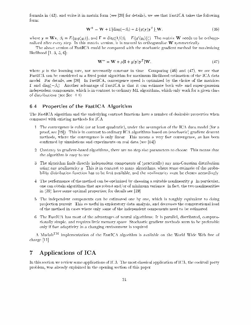
�� The convergence is cubic �or at least quadratic�� under the assumption of the ICA data model �for aproof� see ����� This is in contrast to ordinary ICA algorithms based on �stochastic� gradient descentmethods� where the convergence is only linear� This means a very fast convergence� as has beencon�rmed by simulations and experiments on real data �see �����

�� Contrary to gradient�based algorithms� there are no step size parameters to choose� This means thatthe algorithm is easy to use�

�� The algorithm �nds directly independent components of �practically� any non�Gaussian distributionusing any nonlinearity g� This is in contrast to many algorithms� where some estimate of the proba�bility distribution function has to be �rst available� and the nonlinearity must be chosen accordingly�

�� The performance of the method can be optimized by choosing a suitable nonlinearity g� In particular�one can obtain algorithms that are robust and�or of minimum variance� In fact� the two nonlinearitiesin ���� have some optimal properties� for details see ����

�� The independent components can be estimated one by one� which is roughly equivalent to doingprojection pursuit� This es useful in exploratory data analysis� and decreases the computational loadof the method in cases where only some of the independent components need to be estimated�

�� The FastICA has most of the advantages of neural algorithms� It is parallel� distributed� computa�tionally simple� and requires little memory space� Stochastic gradient methods seem to be preferableonly if fast adaptivity in a changing environment is required�

A MatlabTM implementation of the FastICA algorithm is available on the World Wide Web free ofcharge ����

� Applications of ICA

In this section we review some applications of ICA� The most classical application of ICA� the cocktail�partyproblem� was already explained in the opening section of this paper�

��

�� Separation of Artifacts in MEG Data

Magnetoencephalography �MEG� is a noninvasive technique by which the activity or the cortical neuronscan be measured with very good temporal resolution and moderate spatial resolution� When using a MEGrecord� as a research or clinical tool� the investigator may face a problem of extracting the essential featuresof the neuromagnetic signals in the presence of artifacts� The amplitude of the disturbances may be higherthan that of the brain signals� and the artifacts may resemble pathological signals in shape�In ���� the authors introduced a new method to separate brain activity from artifacts using ICA� The

approach is based on the assumption that the brain activity and the artifacts� e�g� eye movements orblinks� or sensor malfunctions� are anatomically and physiologically separate processes� and this separationis re�ected in the statistical independence between the magnetic signals generated by those processes� Theapproach follows the earlier experiments with EEG signals� reported in ���� A related approach is that of ����The MEG signals were recorded in a magnetically shielded room with a ����channel whole�scalp

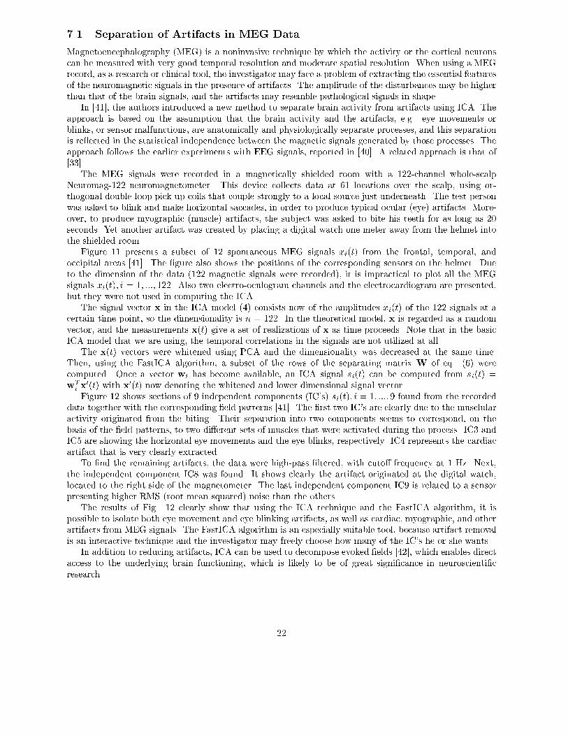
Neuromag���� neuromagnetometer� This device collects data at �� locations over the scalp� using or�thogonal double�loop pick�up coils that couple strongly to a local source just underneath� The test personwas asked to blink and make horizontal saccades� in order to produce typical ocular �eye� artifacts� More�over� to produce myographic �muscle� artifacts� the subject was asked to bite his teeth for as long as ��seconds� Yet another artifact was created by placing a digital watch one meter away from the helmet intothe shielded room�Figure �� presents a subset of �� spontaneous MEG signals xi�t� from the frontal� temporal� and

occipital areas ���� The �gure also shows the positions of the corresponding sensors on the helmet� Dueto the dimension of the data ���� magnetic signals were recorded�� it is impractical to plot all the MEGsignals xi�t�� i � �� ���� ���� Also two electro�oculogram channels and the electrocardiogram are presented�but they were not used in computing the ICA�The signal vector x in the ICA model ��� consists now of the amplitudes xi�t� of the ��� signals at a

certain time point� so the dimensionality is n � ���� In the theoretical model� x is regarded as a randomvector� and the measurements x�t� give a set of realizations of x as time proceeds� Note that in the basicICA model that we are using� the temporal correlations in the signals are not utilized at all�The x�t� vectors were whitened using PCA and the dimensionality was decreased at the same time�

Then� using the FastICA algorithm� a subset of the rows of the separating matrix W of eq� ��� werecomputed� Once a vector wi has become available� an ICA signal si�t� can be computed from si�t� �wTi x

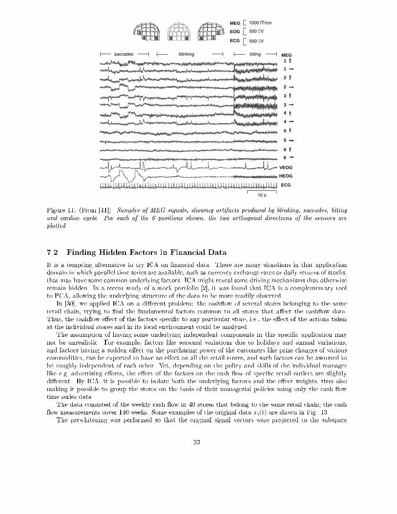
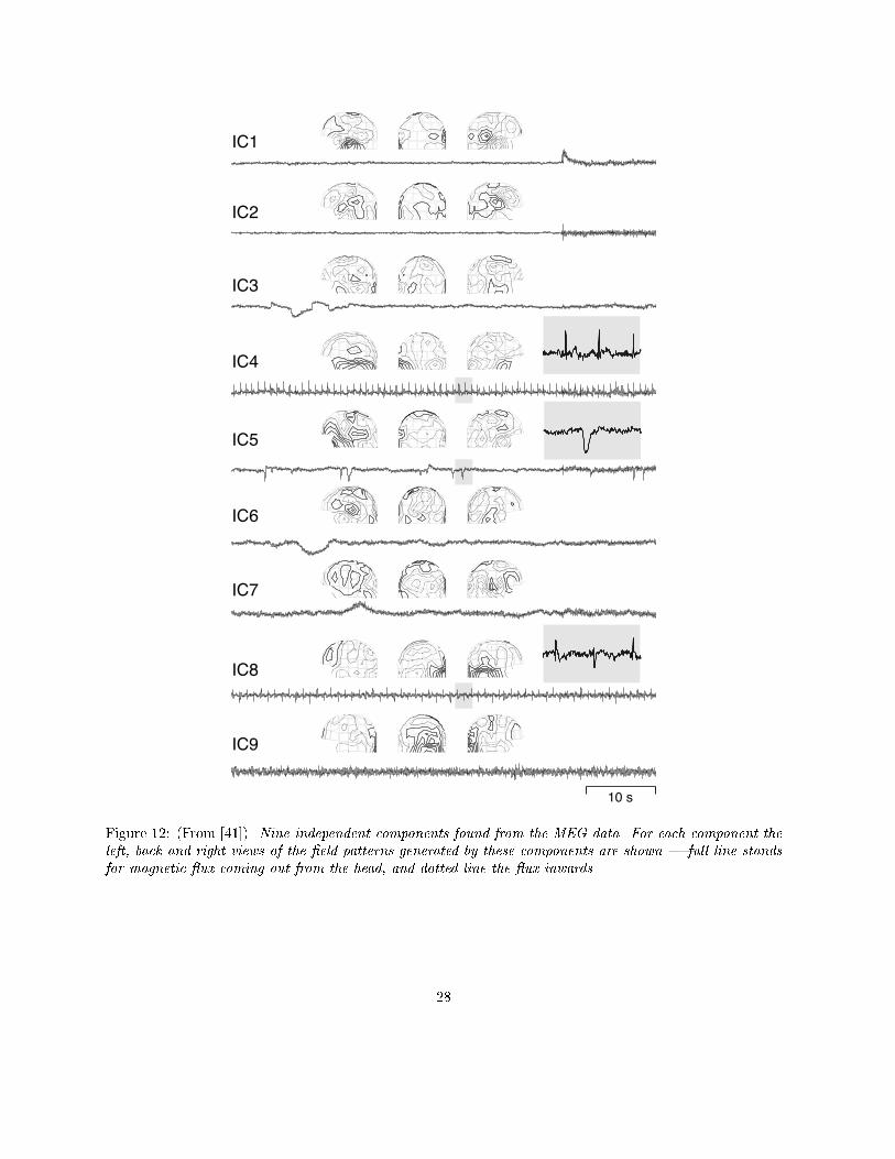
��t� with x��t� now denoting the whitened and lower dimensional signal vector�Figure �� shows sections of � independent components �ICs� si�t�� i � �� ���� � found from the recorded

data together with the corresponding �eld patterns ���� The �rst two ICs are clearly due to the musclularactivity originated from the biting� Their separation into two components seems to correspond� on thebasis of the �eld patterns� to two di�erent sets of muscles that were activated during the process� IC� andIC� are showing the horizontal eye movements and the eye blinks� respectively� IC� represents the cardiacartifact that is very clearly extracted�To �nd the remaining artifacts� the data were high�pass �ltered� with cuto� frequency at � Hz� Next�

the independent component IC� was found� It shows clearly the artifact originated at the digital watch�located to the right side of the magnetometer� The last independent component IC� is related to a sensorpresenting higher RMS �root mean squared� noise than the others�The results of Fig� �� clearly show that using the ICA technique and the FastICA algorithm� it is

possible to isolate both eye movement and eye blinking artifacts� as well as cardiac� myographic� and otherartifacts from MEG signals� The FastICA algorithm is an especially suitable tool� because artifact removalis an interactive technique and the investigator may freely choose how many of the ICs he or she wants�In addition to reducing artifacts� ICA can be used to decompose evoked �elds ���� which enables direct

access to the underlying brain functioning� which is likely to be of great signi�cance in neuroscienti�cresearch�

��

12

63

54

1

1

2

2

3

3

4

4

5

5

6

6

VEOG

ECG

MEG

HEOG

10 s

5 6500 µV

500 µV

1000 fT/cmMEG

EOG

ECG

saccades blinking biting

Figure ��� �From ����� Samples of MEG signals� showing artifacts produced by blinking� saccades� bitingand cardiac cycle� For each of the � positions shown� the two orthogonal directions of the sensors areplotted�

�� Finding Hidden Factors in Financial Data

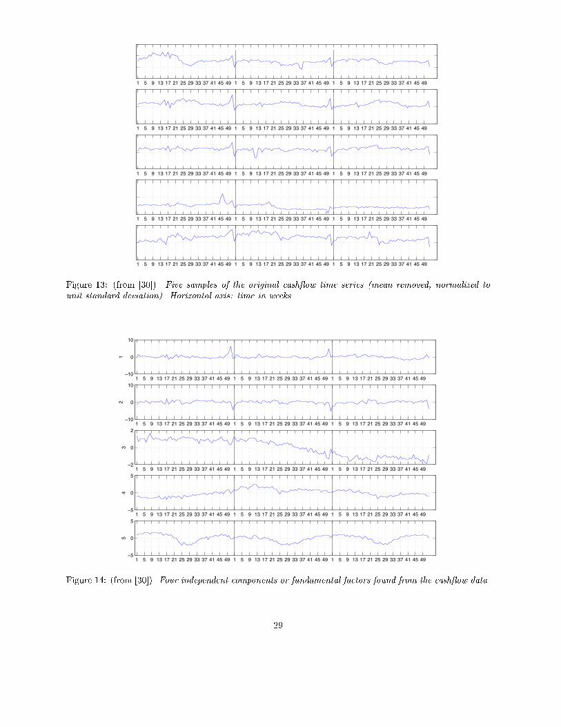
It is a tempting alternative to try ICA on �nancial data� There are many situations in that applicationdomain in which parallel time series are available� such as currency exchange rates or daily returns of stocks�that may have some common underlying factors� ICA might reveal some driving mechanisms that otherwiseremain hidden� In a recent study of a stock portfolio ��� it was found that ICA is a complementary toolto PCA� allowing the underlying structure of the data to be more readily observed�In ���� we applied ICA on a di�erent problem� the cash�ow of several stores belonging to the same

retail chain� trying to �nd the fundamental factors common to all stores that a�ect the cash�ow data�Thus� the cash�ow e�ect of the factors speci�c to any particular store� i�e�� the e�ect of the actions takenat the individual stores and in its local environment could be analyzed�The assumption of having some underlying independent components in this speci�c application may

not be unrealistic� For example� factors like seasonal variations due to holidays and annual variations�and factors having a sudden e�ect on the purchasing power of the customers like prize changes of variouscommodities� can be expected to have an e�ect on all the retail stores� and such factors can be assumed tobe roughly independent of each other� Yet� depending on the policy and skills of the individual managerlike e�g� advertising e�orts� the e�ect of the factors on the cash �ow of speci�c retail outlets are slightlydi�erent� By ICA� it is possible to isolate both the underlying factors and the e�ect weights� thus alsomaking it possible to group the stores on the basis of their managerial policies using only the cash �owtime series data�The data consisted of the weekly cash �ow in �� stores that belong to the same retail chain� the cash

�ow measurements cover ��� weeks� Some examples of the original data xi�t� are shown in Fig� ���The prewhitening was performed so that the original signal vectors were projected to the subspace

��

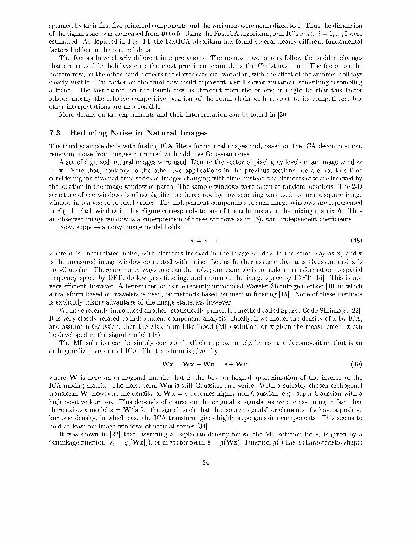
spanned by their �rst �ve principal components and the variances were normalized to �� Thus the dimensionof the signal space was decreased from �� to �� Using the FastICA algorithm� four ICs si�t�� i � �� ���� � wereestimated� As depicted in Fig� ��� the FastICA algorithm has found several clearly di�erent fundamentalfactors hidden in the original data�The factors have clearly di�erent interpretations� The upmost two factors follow the sudden changes

that are caused by holidays etc�� the most prominent example is the Christmas time� The factor on thebottom row� on the other hand� re�ects the slower seasonal variation� with the e�ect of the summer holidaysclearly visible� The factor on the third row could represent a still slower variation� something resemblinga trend� The last factor� on the fourth row� is di�erent from the others� it might be that this factorfollows mostly the relative competitive position of the retail chain with respect to its competitors� butother interpretations are also possible�More details on the experiments and their interpretation can be found in ����

�� Reducing Noise in Natural Images

The third example deals with �nding ICA �lters for natural images and� based on the ICA decomposition�removing noise from images corrupted with additive Gaussian noise�A set of digitized natural images were used� Denote the vector of pixel gray levels in an image window

by x� Note that� contrary to the other two applications in the previous sections� we are not this timeconsidering multivalued time series or images changing with time� instead the elements of x are indexed bythe location in the image window or patch� The sample windows were taken at random locations� The ��Dstructure of the windows is of no signi�cance here� row by row scanning was used to turn a square imagewindow into a vector of pixel values� The independent components of such image windows are representedin Fig� �� Each window in this Figure corresponds to one of the columns ai of the mixing matrix A� Thusan observed image window is a superposition of these windows as in ���� with independent coecients�Now� suppose a noisy image model holds�

z � x� n ����

where n is uncorrelated noise� with elements indexed in the image window in the same way as x� and zis the measured image window corrupted with noise� Let us further assume that n is Gaussian and x isnon�Gaussian� There are many ways to clean the noise� one example is to make a transformation to spatialfrequency space by DFT� do low�pass �ltering� and return to the image space by IDFT ���� This is notvery ecient� however� A better method is the recently introduced Wavelet Shrinkage method ��� in whicha transform based on wavelets is used� or methods based on median �ltering ���� None of these methodsis explicitly taking advantage of the image statistics� however�We have recently introduced another� statistically principled method called Sparse Code Shrinkage ����

It is very closely related to independent component analysis� Brie�y� if we model the density of x by ICA�and assume n Gaussian� then the Maximum Likelihood �ML� solution for x given the measurement z canbe developed in the signal model �����The ML solution can be simply computed� albeit approximately� by using a decomposition that is an

orthogonalized version of ICA� The transform is given by

Wz �Wx�Wn � s�Wn� ����

where W is here an orthogonal matrix that is the best orthognal approximation of the inverse of theICA mixing matrix� The noise term Wn is still Gaussian and white� With a suitably chosen orthogonaltransformW� however� the density ofWx � s becomes highly non�Gaussian� e�g�� super�Gaussian with ahigh positive kurtosis� This depends of course on the original x signals� as we are assuming in fact thatthere exists a model x �WT s for the signal� such that the �source signals� or elements of s have a positivekurtotic density� in which case the ICA transform gives highly supergaussian components� This seems tohold at least for image windows of natural scenes ����It was shown in ��� that� assuming a Laplacian density for si� the ML solution for si is given by a

�shrinkage function� �si � g��Wz�i�� or in vector form� �s � g�Wz�� Function g��� has a characteristic shape�

��

it is zero close to the origin and then linear after a cutting value depending on the parameters of theLaplacian density and the Gaussian noise density� Assuming other forms for the densities� other optimalshrinkage functions can be derived ����In the Sparse Code Shrinkage method� the shrinkage operation is performed in the rotated space� after

which the estimate for the signal in the original space is given by rotating back�

�x �WT�s �WT g�Wz�� ����

Thus we get the Maximum Likelihood estimate for the image window x in which much of the noise hasbeen removed�The rotation operator W is such that the sparsity of the components s � Wx is maximized� This

operator can be learned with a modi�cation of the FastICA algorithm� see ��� for details�A noise cleaning result is shown in Fig� ��� A noiseless image and a noisy version� in which the noise

level is �� � of the signal level� are shown� The results of the Sparse Code Shrinkage method and classicwiener �ltering are given� indicating that Sparse Code Shrinkage may be a promising approach� The noiseis reduced without blurring edges or other sharp features as much as in wiener �ltering� This is largelydue to the strongly nonlinear nature of the shrinkage operator� that is optimally adapted to the inherentstatistics of natural images�

�� Telecommunications

Finally� we mention another emerging application area of great potential� telecommunications� An exampleof a real�world communications application where blind separation techniques are useful is the separationof the users own signal from the interfering other users signals in CDMA �Code�Division Multiple Access�mobile communications ���� This problem is semi�blind in the sense that certain additional prior informa�tion is available on the CDMA data model� But the number of parameters to be estimated is often so highthat suitable blind source separation techniques taking into account the available prior knowledge providea clear performance improvement over more traditional estimation techniques ����

� Conclusion

ICA is a very general�purpose statistical technique in which observed random data are linearly transformedinto components that are maximally independent from each other� and simultaneously have �interesting�distributions� ICA can be formulated as the estimation of a latent variable model� The intuitive notion ofmaximum nongaussianity can be used to derive di�erent objective functions whose optimization enables theestimation of the ICA model� Alternatively� one may use more classical notions like maximum likelihoodestimation or minimization of mutual information to estimate ICA� somewhat surprisingly� these approachesare �approximatively� equivalent� A computationally very ecient method performing the actual estimationis given by the FastICA algorithm� Applications of ICA can be found in many di�erent areas such as audioprocessing� biomedical signal processing� image processing� telecommunications� and econometrics�

References

�� S��I� Amari� A� Cichocki� and H�H� Yang� A new learning algorithm for blind source separation� InAdvances in Neural Information Processing Systems �� pages �������� MIT Press� Cambridge� MA������

�� A� D� Back and A� S� Weigend� A �rst application of independent component analysis to extractingstructure from stock returns� Int� J� on Neural Systems� ������������� �����

�� A�J� Bell and T�J� Sejnowski� An information�maximization approach to blind separation and blinddeconvolution� Neural Computation� ������������ �����

��

�� J��F� Cardoso� Infomax and maximum likelihood for source separation� IEEE Letters on SignalProcessing� ���������� �����

�� J��F� Cardoso and B� Hvam Laheld� Equivariant adaptive source separation� IEEE Trans� on SignalProcessing� ����������������� �����

�� A� Cichocki� R�E� Bogner� L� Moszczynski� and K� Pope� Modi�ed Herault�Jutten algorithms for blindseparation of sources� Digital Signal Processing� ���� � ��� �����

�� P� Comon� Independent component analysis � a new concept� Signal Processing� ����������� �����

�� T� M� Cover and J� A� Thomas� Elements of Information Theory� John Wiley Sons� �����

�� N� Delfosse and P� Loubaton� Adaptive blind separation of independent sources� a de�ation approach�Signal Processing� ��������� �����

��� D� L� Donoho� I� M� Johnstone� G� Kerkyacharian� and D� Picard� Wavelet shrinkage� asymptopia�Journal of the Royal Statistical Society ser� B� ����������� �����

��� The FastICA MATLAB package� Available at http���www�cis�hut�fi�projects�ica�fastica��

��� J� H� Friedman and J� W� Tukey� A projection pursuit algorithm for exploratory data analysis� IEEETrans� of Computers� c��������������� �����

��� J�H� Friedman� Exploratory projection pursuit� J� of the American Statistical Association� ���������������� �����

��� X� Giannakopoulos� J� Karhunen� and E� Oja� Experimental comparison of neural ICA algorithms� InProc� Int� Conf� on Arti�cial Neural Networks �ICANN���� pages �������� Sk!vde� Sweden� �����

��� R� Gonzalez and P� Wintz� Digital Image Processing� Addison�Wesley� �����

��� P�J� Huber� Projection pursuit� The Annals of Statistics� �������������� �����

��� A� Hyv"rinen� Independent component analysis in the presence of gaussian noise by maximizing jointlikelihood� Neurocomputing� ��������� �����

��� A� Hyv"rinen� New approximations of di�erential entropy for independent component analysis andprojection pursuit� In Advances in Neural Information Processing Systems� volume ��� pages ��������MIT Press� �����

��� A� Hyv"rinen� Fast and robust �xed�point algorithms for independent component analysis� IEEETrans� on Neural Networks� �������������� �����

��� A� Hyv"rinen� The �xed�point algorithm and maximum likelihood estimation for independent compo�nent analysis� Neural Processing Letters� ���������� �����

��� A� Hyv"rinen� Gaussian moments for noisy independent component analysis� IEEE Signal ProcessingLetters� ������������� �����

��� A� Hyv"rinen� Sparse code shrinkage� Denoising of nongaussian data by maximum likelihood estima�tion� Neural Computation� ���������������� �����

��� A� Hyv"rinen� Survey on independent component analysis� Neural Computing Surveys� ��������� �����

��� A� Hyv"rinen and E� Oja� A fast �xed�point algorithm for independent component analysis� NeuralComputation� ��������������� �����

��� A� Hyv"rinen and E� Oja� Independent component analysis by general nonlinear Hebbian�like learningrules� Signal Processing� �������������� �����

��

��� A� Hyv"rinen� J� S"rel"� and R� Vig#rio� Spikes and bumps� Artefacts generated by independentcomponent analysis with insucient sample size� In Proc� Int� Workshop on Independent ComponentAnalysis and Signal Separation �ICA���� pages �������� Aussois� France� �����

��� M�C� Jones and R� Sibson� What is projection pursuit � J� of the Royal Statistical Society� ser� A���������� �����

��� C� Jutten and J� Herault� Blind separation of sources� part I� An adaptive algorithm based on neu�romimetic architecture� Signal Processing� �������� �����

��� J� Karhunen� E� Oja� L� Wang� R� Vig#rio� and J� Joutsensalo� A class of neural networks for inde�pendent component analysis� IEEE Trans� on Neural Networks� ������������� �����

��� K� Kiviluoto and E� Oja� Independent component analysis for parallel �nancial time series� In Proc�ICONIP���� volume �� pages �������� Tokyo� Japan� �����

��� T��W� Lee� M� Girolami� and T� J� Sejnowski� Independent component analysis using an extendedinfomax algorithm for mixed sub�gaussian and super�gaussian sources� Neural Computation� �������������� �����

��� D� G� Luenberger� Optimization by Vector Space Methods� John Wiley Sons� �����

��� S� Makeig� A�J� Bell� T��P� Jung� and T��J� Sejnowski� Independent component analysis of electroen�cephalographic data� In Advances in Neural Information PRocessing Systems �� pages �������� MITPress� �����

��� S� G� Mallat� A theory for multiresolution signal decomposition� The wavelet representation� IEEETrans� on PAMI� ����������� �����

��� J��P� Nadal and N� Parga� Non�linear neurons in the low noise limit� a factorial code maximizesinformation transfer� Network� ���������� �����

��� A� Papoulis� Probability� Random Variables� and Stochastic Processes� McGraw�Hill� �rd edition� �����

��� B� A� Pearlmutter and L� C� Parra� Maximum likelihood blind source separation� A context�sensitivegeneralization of ica� In Advances in Neural Information Processing Systems� volume �� pages �������������

��� D��T� Pham� P� Garrat� and C� Jutten� Separation of a mixture of independent sources through amaximum likelihood approach� In Proc� EUSIPCO� pages �������� �����

��� T� Ristaniemi and J� Joutsensalo� On the performance of blind source separation in CDMA downlink�In Proc� Int� Workshop on Independent Component Analysis and Signal Separation �ICA���� pages�������� Aussois� France� �����

��� R� Vig#rio� Extraction of ocular artifacts from EEG using independent component analysis� Electroen�ceph� clin� Neurophysiol�� ��������������� �����

��� R� Vig#rio� V� Jousm"ki� M� H"m"l"inen� R� Hari� and E� Oja� Independent component analysis foridenti�cation of artifacts in magnetoencephalographic recordings� In Advances in Neural InformationProcessing Systems �� pages �������� MIT Press� �����

��� R� Vig#rio� J� S"rel"� and E� Oja� Independent component analysis in wave decomposition of auditoryevoked �elds� In Proc� Int� Conf� on Arti�cial Neural Networks �ICANN���� pages �������� Sk!vde�Sweden� �����

��

IC1

IC2

IC3

IC4

IC5

IC6

IC7

IC8

IC9

10 s

Figure ��� �From ����� Nine independent components found from the MEG data� For each component theleft� back and right views of the �eld patterns generated by these components are shown � full line standsfor magnetic ux coming out from the head� and dotted line the ux inwards�

��

1 5 9 13 17 21 25 29 33 37 41 45 49 1 5 9 13 17 21 25 29 33 37 41 45 49 1 5 9 13 17 21 25 29 33 37 41 45 49

1 5 9 13 17 21 25 29 33 37 41 45 49 1 5 9 13 17 21 25 29 33 37 41 45 49 1 5 9 13 17 21 25 29 33 37 41 45 49

1 5 9 13 17 21 25 29 33 37 41 45 49 1 5 9 13 17 21 25 29 33 37 41 45 49 1 5 9 13 17 21 25 29 33 37 41 45 49

1 5 9 13 17 21 25 29 33 37 41 45 49 1 5 9 13 17 21 25 29 33 37 41 45 49 1 5 9 13 17 21 25 29 33 37 41 45 49

1 5 9 13 17 21 25 29 33 37 41 45 49 1 5 9 13 17 21 25 29 33 37 41 45 49 1 5 9 13 17 21 25 29 33 37 41 45 49

Figure ��� �from ����� Five samples of the original cash ow time series �mean removed� normalized tounit standard deviation� Horizontal axis� time in weeks�

1 5 9 13 17 21 25 29 33 37 41 45 49 1 5 9 13 17 21 25 29 33 37 41 45 49 1 5 9 13 17 21 25 29 33 37 41 45 49−10

0

10

1

1 5 9 13 17 21 25 29 33 37 41 45 49 1 5 9 13 17 21 25 29 33 37 41 45 49 1 5 9 13 17 21 25 29 33 37 41 45 49−10

0

10

2

1 5 9 13 17 21 25 29 33 37 41 45 49 1 5 9 13 17 21 25 29 33 37 41 45 49 1 5 9 13 17 21 25 29 33 37 41 45 49−2

0

2

3

1 5 9 13 17 21 25 29 33 37 41 45 49 1 5 9 13 17 21 25 29 33 37 41 45 49 1 5 9 13 17 21 25 29 33 37 41 45 49−5

0

5

4

1 5 9 13 17 21 25 29 33 37 41 45 49 1 5 9 13 17 21 25 29 33 37 41 45 49 1 5 9 13 17 21 25 29 33 37 41 45 49−5

0

5

5

Figure ��� �from ����� Four independent components or fundamental factors found from the cash ow data�

��

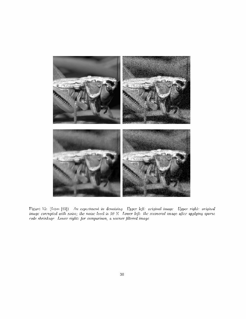
Figure ��� �from ����� An experiment in denoising� Upper left� original image� Upper right� originalimage corrupted with noise� the noise level is �� �� Lower left� the recovered image after applying sparsecode shrinkage� Lower right� for comparison� a wiener �ltered image�

��