Embed Size (px)
Citation preview

Page 1 of 29
1. Background In close collaboration with local partners, Earthquake Damage Analysis Center (EDAC) of
Bauhaus‐Universität Weimar initiated a Turkish‐German joint research project on Seismic Risk
Assessment and Mitigation in the Antakya‐Maraş‐Region (SERAMAR).
In this context, the instrumental investigation of buildings being representative for the study
area becomes an essential part of the project to calibrate the models and to predict reliable
capacity curves as well as scenario‐dependent damage pattern or failure modes. Based on
different decision criteria, three multistory RC frame structures have been chosen and equipped
with modern Seismic Building Monitoring Systems (BMS) each of which consists of four triaxial
strong‐motion accelerometers of type MR2002+. After a 2 year test period, first results from the
permanent instrumentation are available and provide a preliminary basis to reinterpret the
structural response under seismic action.
Into the project one of these buildings (see Fig.1 and 2) will be investigated and measured data
will be analyzed in detail.
The main purpose of this project will be to apply as much of the theoretical background taught
during the lessons on Earthquake Engineering and Structural Design and Seismic Monitoring.
2. Objectives of Project
- The interpretation of the structural system in view of earthquake resistance (ERD).
- The design and analysis of the structural system using the software ETABS Nonlinear for
the given building layout with (a) and without (b) masonry infill walls.
- The analysis of the instrumental vibration data in order to identify dynamic structural
parameters.
- The comparison of the experimentally gained results with outcomes of the structural
analysis.
- The proposal of strengthening and retrofitting measures.
Page 2 of 29
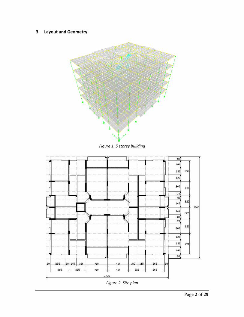
3. Layout and Geometry
Figure 1. 5 storey building
Figure 2. Site plan
Page 3 of 29
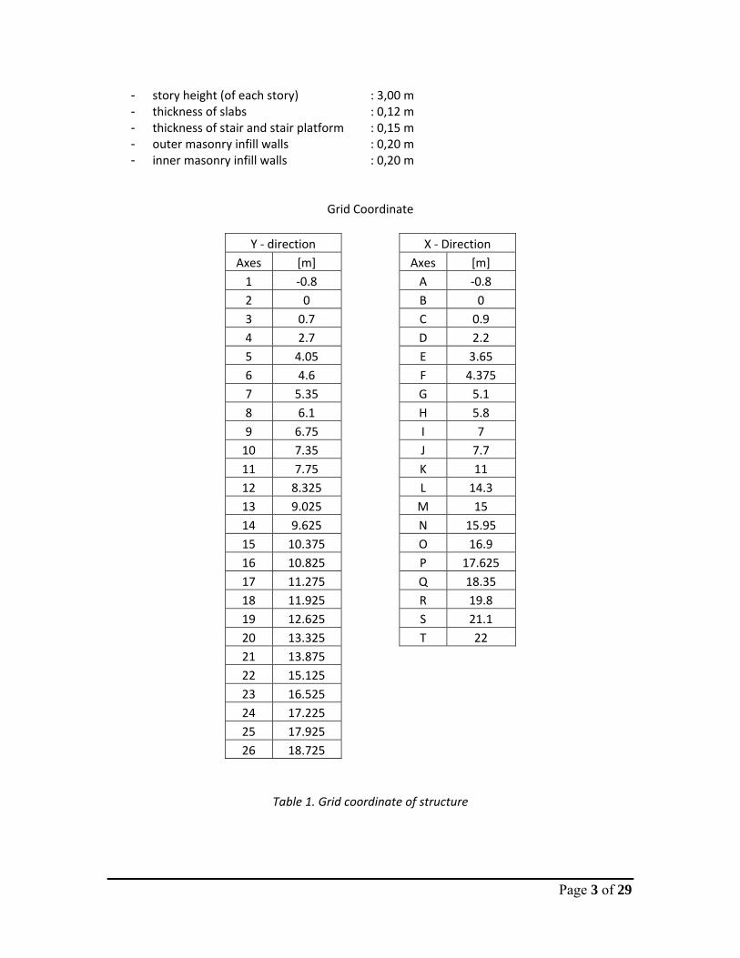
- story height (of each story) : 3,00 m - thickness of slabs : 0,12 m - thickness of stair and stair platform : 0,15 m - outer masonry infill walls : 0,20 m - inner masonry infill walls : 0,20 m
Grid Coordinate
Y ‐ direction X ‐ Direction Axes [m] Axes [m] 1 ‐0.8 A ‐0.8 2 0 B 0 3 0.7 C 0.9 4 2.7 D 2.2 5 4.05 E 3.65 6 4.6 F 4.375 7 5.35 G 5.1 8 6.1 H 5.8 9 6.75 I 7 10 7.35 J 7.7 11 7.75 K 11 12 8.325 L 14.3 13 9.025 M 15 14 9.625 N 15.95 15 10.375 O 16.9 16 10.825 P 17.625 17 11.275 Q 18.35 18 11.925 R 19.8 19 12.625 S 21.1 20 13.325 T 22 21 13.875 22 15.125 23 16.525 24 17.225 25 17.925 26 18.725
Table 1. Grid coordinate of structure
Page 4 of 29
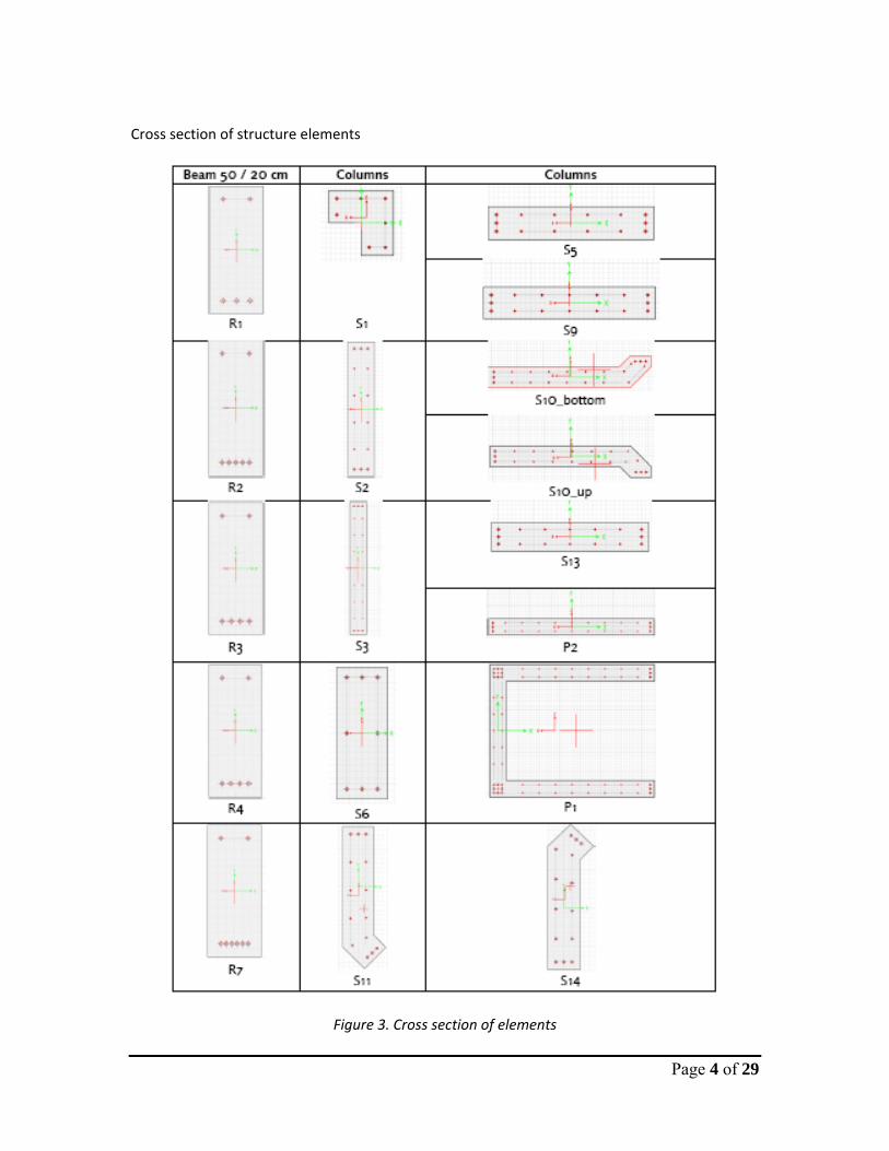
Cross section of structure elements
Figure 3. Cross section of elements
Page 5 of 29
4. Material Properties Reinforced Concrete : Young´s modulus : 2,80e+07 kN/m² Poisson ratio : 0,2 Mass density : 2,55 t/m³ Weight : 25 kN/m³ Concrete Strength : 25.000 kN/m² Steel Strength : 420.000 kN/m² Masonry: Young´s modulus : 2.1e+6 kN/m² Poisson ratio : 0,15 Mass density : 0,918 t/m³ Weight : 9,0 kN/m³ Masonry Strength : 0.60 MN/m² 5. Loads
5.1 Dead Load and Live Load
Based on the purpose of the project the following loads will be applied: 2,0 kN/m² on the roof as load for the roof construction 1,0 kN/m² on the floor slabs as load for interior etc.
For the purpose of strengthening and retrofitting it’s necessary to apply loads according to the requirements from EC 1 and the application of the load combinations according to EC 8.
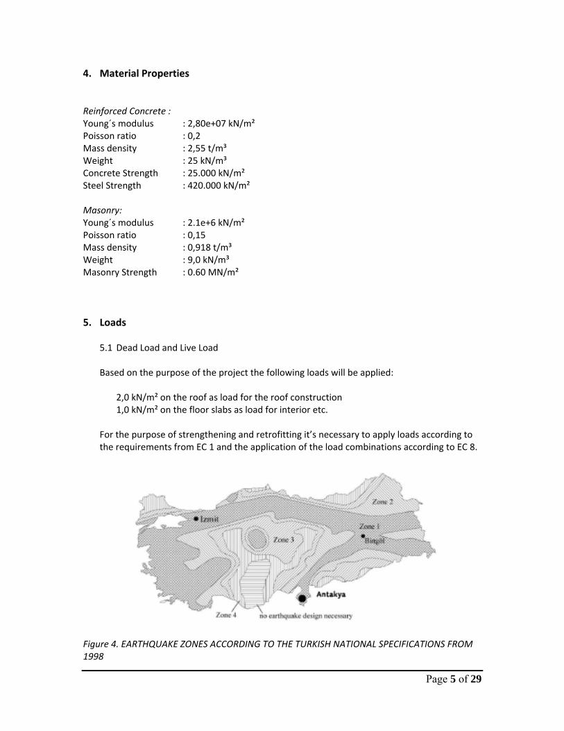
Figure 4. EARTHQUAKE ZONES ACCORDING TO THE TURKISH NATIONAL SPECIFICATIONS FROM 1998
Page 6 of 29
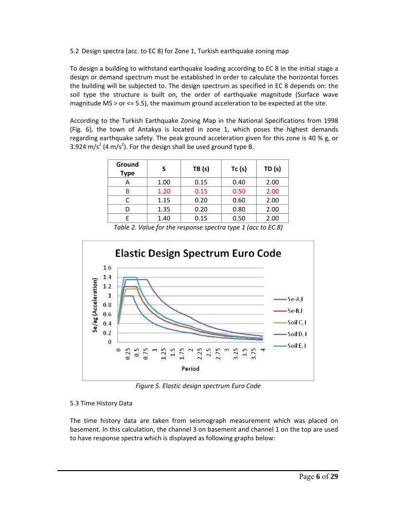
5.2 Design spectra (acc. to EC 8) for Zone 1, Turkish earthquake zoning map
To design a building to withstand earthquake loading according to EC 8 in the initial stage a design or demand spectrum must be established in order to calculate the horizontal forces the building will be subjected to. The design spectrum as specified in EC 8 depends on: the soil type the structure is built on, the order of earthquake magnitude (Surface wave magnitude MS > or <= 5.5), the maximum ground acceleration to be expected at the site. According to the Turkish Earthquake Zoning Map in the National Specifications from 1998 (Fig. 6), the town of Antakya is located in zone 1, which poses the highest demands regarding earthquake safety. The peak ground acceleration given for this zone is 40 % g, or 3.924 m/s2 (4 m/s2). For the design shall be used ground type B.
Ground Type
S TB (s) Tc (s) TD (s)
A 1.00 0.15 0.40 2.00 B 1.20 0.15 0.50 2.00 C 1.15 0.20 0.60 2.00 D 1.35 0.20 0.80 2.00 E 1.40 0.15 0.50 2.00
Table 2. Value for the response spectra type 1 (acc to EC.8)
Figure 5. Elastic design spectrum Euro Code
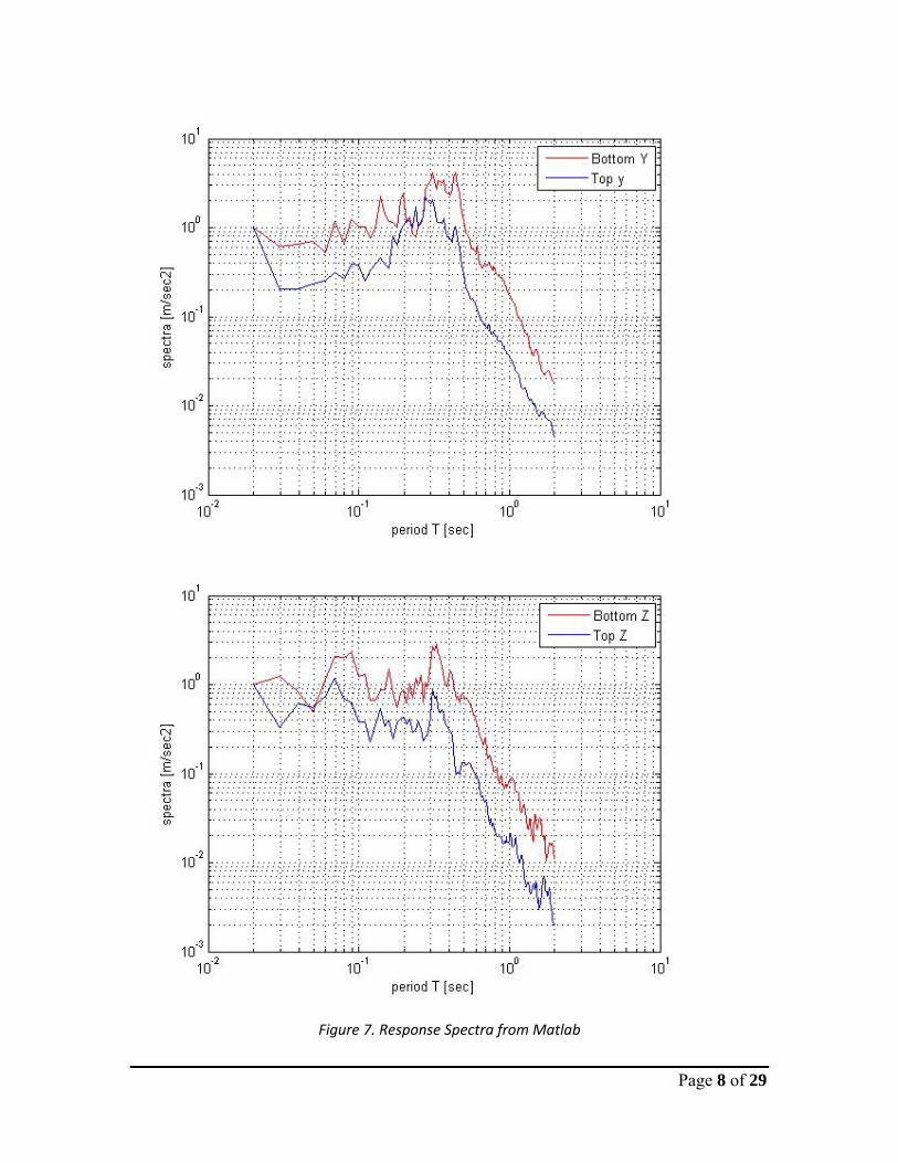
5.3 Time History Data
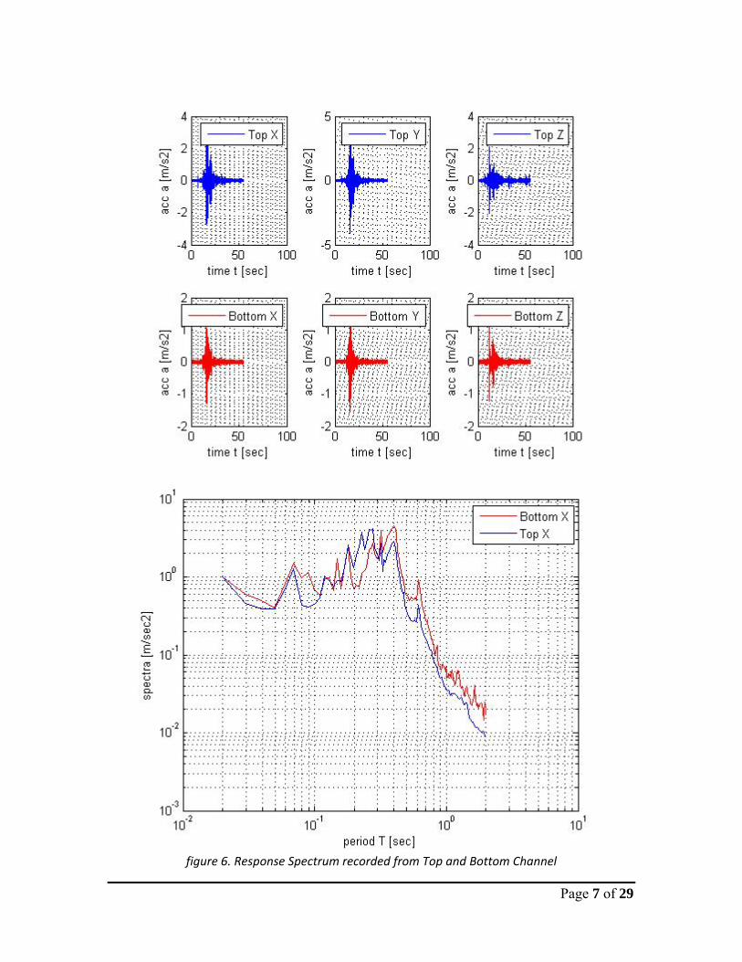
The time history data are taken from seismograph measurement which was placed on basement. In this calculation, the channel 3 on basement and channel 1 on the top are used to have response spectra which is displayed as following graphs below:
Page 7 of 29
figure 6. Response Spectrum recorded from Top and Bottom Channel
Page 8 of 29
Figure 7. Response Spectra from Matlab
Page 9 of 29
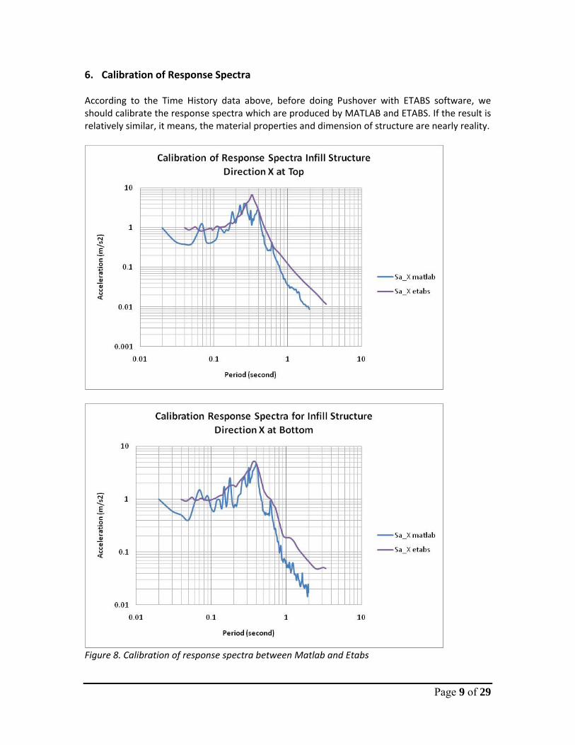
6. Calibration of Response Spectra According to the Time History data above, before doing Pushover with ETABS software, we should calibrate the response spectra which are produced by MATLAB and ETABS. If the result is relatively similar, it means, the material properties and dimension of structure are nearly reality.
Figure 8. Calibration of response spectra between Matlab and Etabs
Page 10 of 29
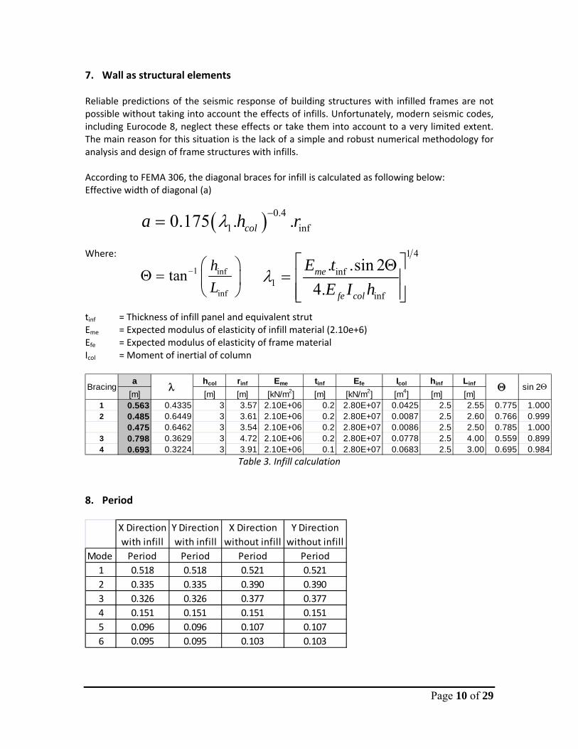
7. Wall as structural elements Reliable predictions of the seismic response of building structures with infilled frames are not possible without taking into account the effects of infills. Unfortunately, modern seismic codes, including Eurocode 8, neglect these effects or take them into account to a very limited extent. The main reason for this situation is the lack of a simple and robust numerical methodology for analysis and design of frame structures with infills. According to FEMA 306, the diagonal braces for infill is calculated as following below: Effective width of diagonal (a) Where: tinf = Thickness of infill panel and equivalent strut Eme = Expected modulus of elasticity of infill material (2.10e+6) Efe = Expected modulus of elasticity of frame material Icol = Moment of inertial of column
a hcol rinf Eme tinf Efe Icol hinf Linf
[m] [m] [m] [kN/m2] [m] [kN/m2] [m4] [m] [m]1 0.563 0.4335 3 3.57 2.10E+06 0.2 2.80E+07 0.0425 2.5 2.55 0.775 1.0002 0.485 0.6449 3 3.61 2.10E+06 0.2 2.80E+07 0.0087 2.5 2.60 0.766 0.999
0.475 0.6462 3 3.54 2.10E+06 0.2 2.80E+07 0.0086 2.5 2.50 0.785 1.0003 0.798 0.3629 3 4.72 2.10E+06 0.2 2.80E+07 0.0778 2.5 4.00 0.559 0.8994 0.693 0.3224 3 3.91 2.10E+06 0.1 2.80E+07 0.0683 2.5 3.00 0.695 0.984
λ Θ sin 2ΘBracing
Table 3. Infill calculation
8. Period
X Direction with infill
Y Direction with infill
X Direction without infill
Y Direction without infill
Mode Period Period Period Period1 0.518 0.518 0.521 0.5212 0.335 0.335 0.390 0.3903 0.326 0.326 0.377 0.3774 0.151 0.151 0.151 0.1515 0.096 0.096 0.107 0.1076 0.095 0.095 0.103 0.103
( ) 0.41 inf0.175 . .cola h rλ −=
1 4
inf1
inf
. .sin 24.me
fe col
E tE I h
λ⎡ ⎤Θ
= ⎢ ⎥⎢ ⎥⎣ ⎦
1 inf
inf
tanhL
− ⎛ ⎞Θ = ⎜ ⎟
⎝ ⎠

Page 11 of 29
9. Pushover Design
9.1 Capacity Spectrum Method
To use the capacity spectrum method it is necessary to convert the capacity curve, which is
in terms of base shear and roof displacement to what is called a capacity spectrum, which is
a representation of the capacity curve in Acceleration‐Displacement Response Spectra
(ADRS) format. The required equations to make the transformation are:
Where:
MPF1 = Modal Participation Factor for the first natural mode. α1 = modal mass coefficient for the first natural mode Wi/g = mass assigned to level i φi1 = amplitude of mode 1 at level i N = Level N, the level which is the uppermost in the main portion of the structure. V = base shear W = Building load weight plus likely live loads Δroof = roof displacement (V and the associated Δroof make up points on the capacity curve Sa = Spectral acceleration Sd = Spectral displacement (Sa and the associated Sd make up points on the capacity spectrum
9.2 Demand Spectrum
The general process for converting the capacity curve to the capacity spectrum, that is,
converting the capacity curve into the ADRS format, is to first calculate the modal
participation factor (MPF1) and the modal mass coefficient a1 using equation above. Then
for each point on the capacity curve, V, droof, calculate the associated point Sa, Sd on the
capacity spectrum using equations above too.
In the ADRS format, lines radiating from the origin have constant period. For any point on
the ADRS spectrum, the period, T, can be computed using
2
1
21
1 1
i i iN N
ii i
i i
m
w mg
φα
φ= =
⎡ ⎤⎣ ⎦=⎡ ⎤ ⎡ ⎤⎢ ⎥ ⎢ ⎥
⎣ ⎦⎣ ⎦
∑
∑ ∑1
1 1 21
i i
i i
mMPF
mφ
γφ
= = ∑∑
1a bS Vg w α
=1 1
roofd
roof
SMPFϕ
Δ=
Page 12 of 29
2 22 4d d
a a
S ST TS S
π π= → =
Then the spectral displacement is 2
24a
dT SS
π=
When period in the inelastic displacement, the relation between spectral acceleration and
displacement is
2 2 22
2 22
9,81 0.2484 *42
a v v v a v v
d d dd
aa
S C C C S C x CSaSg T g g S SSSS
πππ= = → = → = =
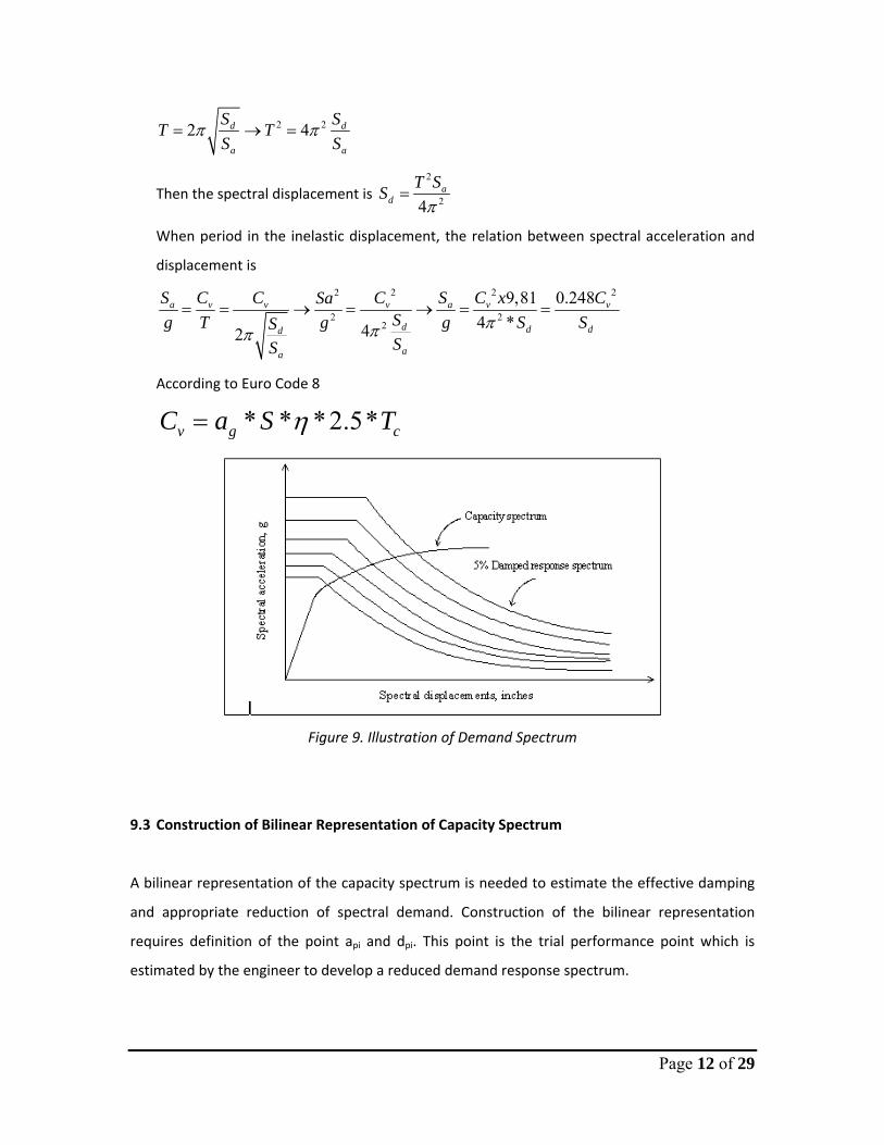
According to Euro Code 8
* * *2.5*v g cC a S Tη=
Figure 9. Illustration of Demand Spectrum
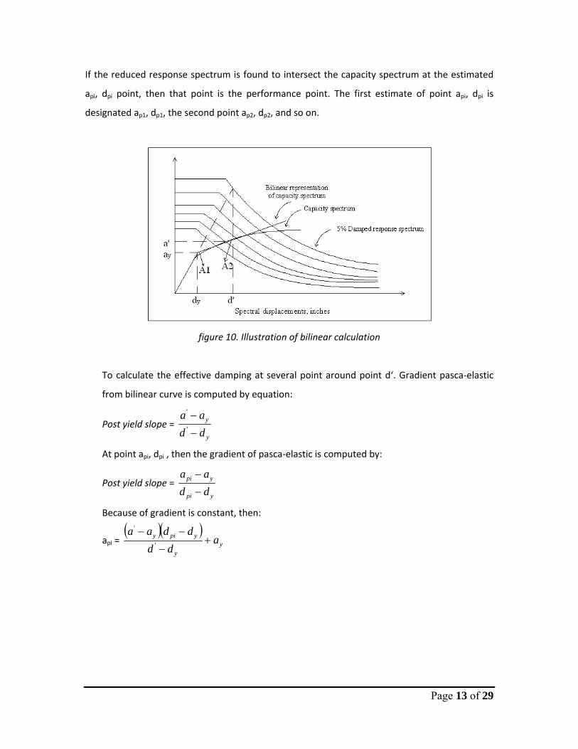
9.3 Construction of Bilinear Representation of Capacity Spectrum
A bilinear representation of the capacity spectrum is needed to estimate the effective damping
and appropriate reduction of spectral demand. Construction of the bilinear representation
requires definition of the point api and dpi. This point is the trial performance point which is
estimated by the engineer to develop a reduced demand response spectrum.
Page 13 of 29
If the reduced response spectrum is found to intersect the capacity spectrum at the estimated
api, dpi point, then that point is the performance point. The first estimate of point api, dpi is
designated ap1, dp1, the second point ap2, dp2, and so on.
figure 10. Illustration of bilinear calculation
To calculate the effective damping at several point around point d‘. Gradient pasca‐elastic
from bilinear curve is computed by equation:
Post yield slope = y
y
ddaa
−
−'
'
At point api, dpi , then the gradient of pasca‐elastic is computed by:
Post yield slope = ypi
ypi
ddaa
−
−
Because of gradient is constant, then:
api = ( )( )
yy
ypiy add
ddaa+
−
−−'
'
Page 14 of 29
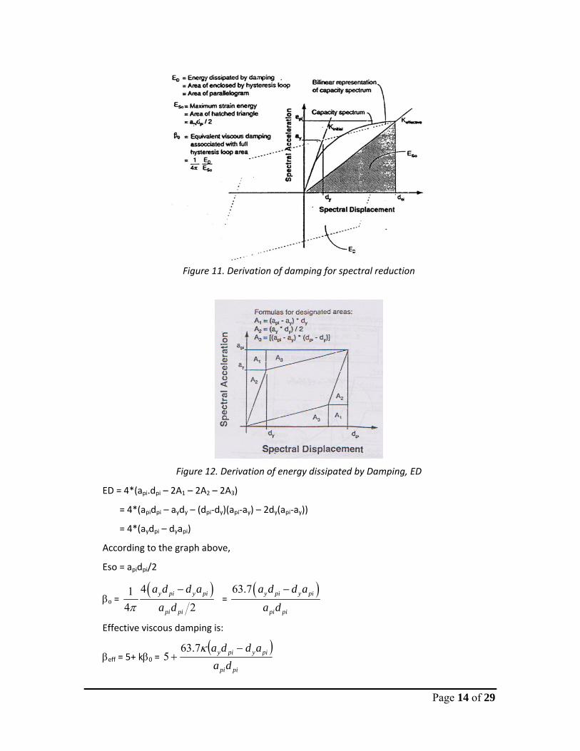
Figure 11. Derivation of damping for spectral reduction
Figure 12. Derivation of energy dissipated by Damping, ED
ED = 4*(api.dpi – 2A1 – 2A2 – 2A3)
= 4*(apidpi – aydy – (dpi‐dy)(api‐ay) – 2dy(api‐ay))
= 4*(aydpi – dyapi)
According to the graph above,
Eso = apidpi/2
βo = ( )41
4 2y pi y pi
pi pi
a d d aa dπ
− =
( )63.7 y pi y pi
pi pi
a d d aa d
−
Effective viscous damping is:
βeff = 5+ kβ0 = ( )
pipi
piypiy
daadda −
+κ7.63
5
Page 15 of 29
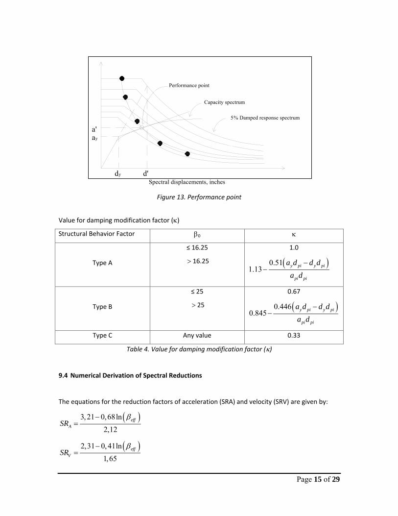
Spectral displacements, inchesdy d'
a'ay
Capacity spectrum
5% Damped response spectrum
Performance point
Figure 13. Performance point
Value for damping modification factor (κ)
Structural Behavior Factor β0 κ
Type A
≤ 16.25
> 16.25
1.0
( )0.511.13 y pi y pi
pi pi
a d d da d
−−
Type B
≤ 25
> 25
0.67
( )0.4460.845 y pi y pi
pi pi
a d d da d
−−
Type C Any value 0.33
Table 4. Value for damping modification factor (κ)
9.4 Numerical Derivation of Spectral Reductions
The equations for the reduction factors of acceleration (SRA) and velocity (SRV) are given by:
( )3, 21 0,68ln2,12
effASR
β−=
( )2,31 0, 41ln1,65
effVSR
β−=
Page 16 of 29
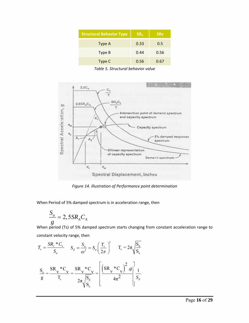
Structural Behavior Type SRA SRv
Type A 0.33 0.5
Type B 0.44 0.56
Type C 0.56 0.67
Table 5. Structural behavior value
Figure 14. illustration of Performance point determination
When Period of 5% damped spectrum is in acceleration range, then
When period (Ts) of 5% damped spectrum starts changing from constant acceleration range to
constant velocity range, then
( )a
s d
a
2SR *C .SR *C SR *CS 1v vv v v v= = = 2g T S 4π2π
Sd
g
S
⎡ ⎤⎢ ⎥⎢ ⎥⎢ ⎥⎢ ⎥⎣ ⎦
*v vs
a
SR CT
S=
2
2 2a s
d aS T
S Sπω
⎛ ⎞= = ⎜ ⎟⎝ ⎠
ds
a
ST = 2πS
2,5aA A
SSR C
g=

Page 17 of 29
9.5 Pushover Methods
In the general case, determination of the performance point requires a trial and error search.
There are three different procedures that standardize and simplify this iterative process. These
alternate procedures are all based on the same concepts and mathematical relationships but
vary in their dependence on analytical versus graphical techniques. These procedures are
following below:
1. Procedure A
Procedure A is truly iterative, but is formula‐based and easily can be programmed into a
spreadsheet. It is more an analytical method than a graphical method. It may be the
best method for beginners because it is the most direct application of the methodology,
and consequently is the easiest procedure to understand.
2. Procedure B
Simplification is introduced in the bilinear modeling of the capacity curve that enables a
relatively direct solution for the performance point with little iteration. Like procedure
A, procedure B is more an analytical method than a graphical method. Procedure B may
be a less transparent application of the methodology than procedure A.
3. Procedure C
Procedure C is a pure graphical method to find the performance point, similar to the
originally conceived capacity spectrum method, and is consistent with the concepts and
mathematical relationships. It is the most convenient method for hand analysis. It is not
particularly convenient for spreadsheet programming. It is the least transparent
application of the methodology.
10 Push Over Results
10.1 Structure with Infill
10.1.1 X Direction
10.1.1.1 Procedure A
Page 18 of 29
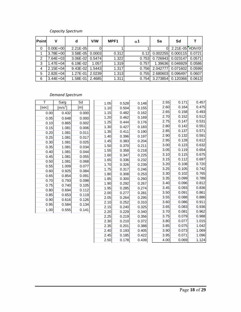
Capacity Spectrum
Point V d V/W MPF1 α1 Sa Sd T
0 0.00E+00 2.21E-05 0 1 1 0 2.21E-05 #DIV/0!1 3.78E+00 3.58E-05 0.0003 0.312 0.12 0.002255 0.000115 0.07212 7.64E+03 3.06E-02 0.5474 1.322 0.753 0.726943 0.023147 0.05713 1.47E+04 6.19E-02 1.057 1.319 0.757 1.39636 0.046929 0.05864 2.15E+04 9.43E-02 1.5443 1.317 0.756 2.042777 0.071602 0.05995 2.82E+04 1.27E-01 2.0239 1.313 0.755 2.680603 0.096497 0.06076 3.44E+04 1.58E-01 2.4685 1.311 0.754 3.273854 0.120366 0.0613
Demand Spectrum
T Sa/g Sd[sec] [m/s2] [m]
0.00 0.432 0.0000.05 0.648 0.0000.10 0.865 0.0020.15 1.081 0.0060.20 1.081 0.0110.25 1.081 0.0170.30 1.081 0.0250.35 1.081 0.0340.40 1.081 0.0440.45 1.081 0.0550.50 1.081 0.0680.55 1.009 0.0770.60 0.925 0.0840.65 0.854 0.0910.70 0.793 0.0980.75 0.740 0.1050.80 0.694 0.1120.85 0.653 0.1190.90 0.616 0.1260.95 0.584 0.1341.00 0.555 0.141
1.05 0.528 0.1481.10 0.504 0.1551.15 0.482 0.1621.20 0.462 0.1691.25 0.444 0.1761.30 0.427 0.1831.35 0.411 0.1901.40 0.396 0.1971.45 0.383 0.2041.50 0.370 0.2111.55 0.358 0.2181.60 0.347 0.2251.65 0.336 0.2321.70 0.326 0.2391.75 0.317 0.2461.80 0.308 0.2531.85 0.300 0.2601.90 0.292 0.2671.95 0.285 0.2742.00 0.277 0.2812.05 0.264 0.2952.10 0.252 0.3102.15 0.240 0.3252.20 0.229 0.3402.25 0.219 0.3562.30 0.210 0.3722.35 0.201 0.3882.40 0.193 0.4052.45 0.185 0.4222.50 0.178 0.439
2.55 0.171 0.4572.60 0.164 0.4752.65 0.158 0.4932.70 0.152 0.5122.75 0.147 0.5312.80 0.142 0.5512.85 0.137 0.5712.90 0.132 0.5912.95 0.128 0.6123.00 0.123 0.6323.05 0.119 0.6543.10 0.115 0.6753.15 0.112 0.6973.20 0.108 0.7203.25 0.105 0.7423.30 0.102 0.7653.35 0.099 0.7893.40 0.096 0.8123.45 0.093 0.8363.50 0.091 0.8613.55 0.088 0.8863.60 0.086 0.9113.65 0.083 0.9363.70 0.081 0.9623.75 0.079 0.9883.80 0.077 1.0153.85 0.075 1.0423.90 0.073 1.0693.95 0.071 1.0964.00 0.069 1.124
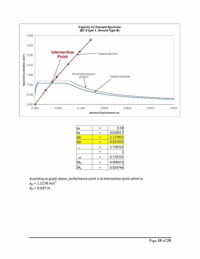
Page 19 of 29
ay = 0.59dy = 0.018517api = 1.117852dpi = 0.037035
�o = 1.770721� = 1
�eff = 6.770721
SRA = 0.900673
SRV = 0.924746
According to graph above, performance point is at intersection point which is: api = 1.1178 m/s2 dpi = 0.037 m
Page 20 of 29
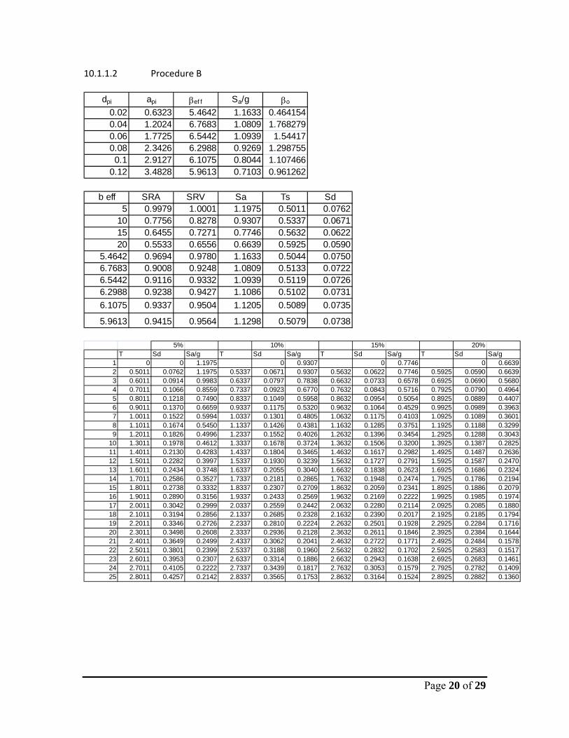
10.1.1.2 Procedure B
dpi api βef f Sa/g βo
0.02 0.6323 5.4642 1.1633 0.4641540.04 1.2024 6.7683 1.0809 1.7682790.06 1.7725 6.5442 1.0939 1.544170.08 2.3426 6.2988 0.9269 1.2987550.1 2.9127 6.1075 0.8044 1.107466
0.12 3.4828 5.9613 0.7103 0.961262
b eff SRA SRV Sa Ts Sd5 0.9979 1.0001 1.1975 0.5011 0.0762
10 0.7756 0.8278 0.9307 0.5337 0.067115 0.6455 0.7271 0.7746 0.5632 0.062220 0.5533 0.6556 0.6639 0.5925 0.0590
5.4642 0.9694 0.9780 1.1633 0.5044 0.07506.7683 0.9008 0.9248 1.0809 0.5133 0.07226.5442 0.9116 0.9332 1.0939 0.5119 0.07266.2988 0.9238 0.9427 1.1086 0.5102 0.07316.1075 0.9337 0.9504 1.1205 0.5089 0.0735
5.9613 0.9415 0.9564 1.1298 0.5079 0.0738
5% 10% 15% 20%T Sd Sa/g T Sd Sa/g T Sd Sa/g T Sd Sa/g
1 0 0 1.1975 0 0.9307 0 0.7746 0 0.66392 0.5011 0.0762 1.1975 0.5337 0.0671 0.9307 0.5632 0.0622 0.7746 0.5925 0.0590 0.66393 0.6011 0.0914 0.9983 0.6337 0.0797 0.7838 0.6632 0.0733 0.6578 0.6925 0.0690 0.56804 0.7011 0.1066 0.8559 0.7337 0.0923 0.6770 0.7632 0.0843 0.5716 0.7925 0.0790 0.49645 0.8011 0.1218 0.7490 0.8337 0.1049 0.5958 0.8632 0.0954 0.5054 0.8925 0.0889 0.44076 0.9011 0.1370 0.6659 0.9337 0.1175 0.5320 0.9632 0.1064 0.4529 0.9925 0.0989 0.39637 1.0011 0.1522 0.5994 1.0337 0.1301 0.4805 1.0632 0.1175 0.4103 1.0925 0.1089 0.36018 1.1011 0.1674 0.5450 1.1337 0.1426 0.4381 1.1632 0.1285 0.3751 1.1925 0.1188 0.32999 1.2011 0.1826 0.4996 1.2337 0.1552 0.4026 1.2632 0.1396 0.3454 1.2925 0.1288 0.3043
10 1.3011 0.1978 0.4612 1.3337 0.1678 0.3724 1.3632 0.1506 0.3200 1.3925 0.1387 0.282511 1.4011 0.2130 0.4283 1.4337 0.1804 0.3465 1.4632 0.1617 0.2982 1.4925 0.1487 0.263612 1.5011 0.2282 0.3997 1.5337 0.1930 0.3239 1.5632 0.1727 0.2791 1.5925 0.1587 0.247013 1.6011 0.2434 0.3748 1.6337 0.2055 0.3040 1.6632 0.1838 0.2623 1.6925 0.1686 0.232414 1.7011 0.2586 0.3527 1.7337 0.2181 0.2865 1.7632 0.1948 0.2474 1.7925 0.1786 0.219415 1.8011 0.2738 0.3332 1.8337 0.2307 0.2709 1.8632 0.2059 0.2341 1.8925 0.1886 0.207916 1.9011 0.2890 0.3156 1.9337 0.2433 0.2569 1.9632 0.2169 0.2222 1.9925 0.1985 0.197417 2.0011 0.3042 0.2999 2.0337 0.2559 0.2442 2.0632 0.2280 0.2114 2.0925 0.2085 0.188018 2.1011 0.3194 0.2856 2.1337 0.2685 0.2328 2.1632 0.2390 0.2017 2.1925 0.2185 0.179419 2.2011 0.3346 0.2726 2.2337 0.2810 0.2224 2.2632 0.2501 0.1928 2.2925 0.2284 0.171620 2.3011 0.3498 0.2608 2.3337 0.2936 0.2128 2.3632 0.2611 0.1846 2.3925 0.2384 0.164421 2.4011 0.3649 0.2499 2.4337 0.3062 0.2041 2.4632 0.2722 0.1771 2.4925 0.2484 0.157822 2.5011 0.3801 0.2399 2.5337 0.3188 0.1960 2.5632 0.2832 0.1702 2.5925 0.2583 0.151723 2.6011 0.3953 0.2307 2.6337 0.3314 0.1886 2.6632 0.2943 0.1638 2.6925 0.2683 0.146124 2.7011 0.4105 0.2222 2.7337 0.3439 0.1817 2.7632 0.3053 0.1579 2.7925 0.2782 0.140925 2.8011 0.4257 0.2142 2.8337 0.3565 0.1753 2.8632 0.3164 0.1524 2.8925 0.2882 0.1360
Page 21 of 29
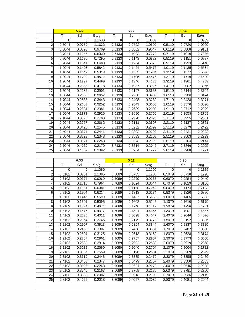
T Sd Sa/g T Sd Sa/g T Sd Sa/g1 0 0 1.1633 0 0 1.0809 0 0 1.09392 0.5044 0.0750 1.1633 0.5133 0.0722 1.0809 0.5119 0.0726 1.09393 0.6044 0.0898 0.9709 0.6133 0.0862 0.9047 0.6119 0.0868 0.91514 0.7044 0.1047 0.8330 0.7133 0.1003 0.7779 0.7119 0.1010 0.78665 0.8044 0.1196 0.7295 0.8133 0.1143 0.6822 0.8119 0.1151 0.68976 0.9044 0.1344 0.6488 0.9133 0.1284 0.6075 0.9119 0.1293 0.61407 1.0044 0.1493 0.5842 1.0133 0.1424 0.5476 1.0119 0.1435 0.55348 1.1044 0.1642 0.5313 1.1133 0.1565 0.4984 1.1119 0.1577 0.50369 1.2044 0.1790 0.4872 1.2133 0.1705 0.4573 1.2119 0.1719 0.4620
10 1.3044 0.1939 0.4499 1.3133 0.1846 0.4225 1.3119 0.1861 0.426811 1.4044 0.2088 0.4178 1.4133 0.1987 0.3926 1.4119 0.2002 0.396612 1.5044 0.2236 0.3901 1.5133 0.2127 0.3667 1.5119 0.2144 0.370413 1.6044 0.2385 0.3657 1.6133 0.2268 0.3439 1.6119 0.2286 0.347414 1.7044 0.2533 0.3443 1.7133 0.2408 0.3239 1.7119 0.2428 0.327115 1.8044 0.2682 0.3252 1.8133 0.2549 0.3060 1.8119 0.2570 0.309016 1.9044 0.2831 0.3081 1.9133 0.2689 0.2900 1.9119 0.2712 0.292917 2.0044 0.2979 0.2928 2.0133 0.2830 0.2756 2.0119 0.2853 0.278318 2.1044 0.3128 0.2788 2.1133 0.2970 0.2626 2.1119 0.2995 0.265119 2.2044 0.3277 0.2662 2.2133 0.3111 0.2507 2.2119 0.3137 0.253120 2.3044 0.3425 0.2546 2.3133 0.3252 0.2399 2.3119 0.3279 0.242221 2.4044 0.3574 0.2441 2.4133 0.3392 0.2299 2.4119 0.3421 0.232222 2.5044 0.3723 0.2343 2.5133 0.3533 0.2208 2.5119 0.3563 0.222923 2.6044 0.3871 0.2253 2.6133 0.3673 0.2123 2.6119 0.3704 0.214424 2.7044 0.4020 0.2170 2.7133 0.3814 0.2045 2.7119 0.3846 0.206525 2.8044 0.4169 0.2092 2.8133 0.3954 0.1972 2.8119 0.3988 0.1991
5.46 6.77 6.54
T Sd Sa/g T Sd Sa/g T Sd Sa/g1 0 0 1.1086 0 0 1.1205 0 0 1.12982 0.5102 0.0731 1.1086 0.5089 0.0735 1.1205 0.5079 0.0738 1.12983 0.6102 0.0874 0.9269 0.6089 0.0879 0.9365 0.6079 0.0884 0.94404 0.7102 0.1018 0.7964 0.7089 0.1024 0.8044 0.7079 0.1029 0.81065 0.8102 0.1161 0.6981 0.8089 0.1168 0.7049 0.8079 0.1174 0.71036 0.9102 0.1304 0.6214 0.9089 0.1313 0.6274 0.9079 0.1320 0.63207 1.0102 0.1447 0.5599 1.0089 0.1457 0.5652 1.0079 0.1465 0.56938 1.1102 0.1591 0.5095 1.1089 0.1602 0.5142 1.1079 0.1610 0.51799 1.2102 0.1734 0.4674 1.2089 0.1746 0.4717 1.2079 0.1756 0.4751
10 1.3102 0.1877 0.4317 1.3089 0.1891 0.4356 1.3079 0.1901 0.438711 1.4102 0.2020 0.4011 1.4089 0.2035 0.4047 1.4079 0.2046 0.407612 1.5102 0.2164 0.3745 1.5089 0.2179 0.3779 1.5079 0.2192 0.380613 1.6102 0.2307 0.3513 1.6089 0.2324 0.3544 1.6079 0.2337 0.356914 1.7102 0.2450 0.3307 1.7089 0.2468 0.3337 1.7079 0.2482 0.336015 1.8102 0.2594 0.3125 1.8089 0.2613 0.3152 1.8079 0.2628 0.317416 1.9102 0.2737 0.2961 1.9089 0.2757 0.2987 1.9079 0.2773 0.300817 2.0102 0.2880 0.2814 2.0089 0.2902 0.2838 2.0079 0.2919 0.285818 2.1102 0.3023 0.2680 2.1089 0.3046 0.2704 2.1079 0.3064 0.272219 2.2102 0.3167 0.2559 2.2089 0.3190 0.2581 2.2079 0.3209 0.259920 2.3102 0.3310 0.2448 2.3089 0.3335 0.2470 2.3079 0.3355 0.248621 2.4102 0.3453 0.2347 2.4089 0.3479 0.2367 2.4079 0.3500 0.238322 2.5102 0.3596 0.2253 2.5089 0.3624 0.2273 2.5079 0.3645 0.228823 2.6102 0.3740 0.2167 2.6089 0.3768 0.2186 2.6079 0.3791 0.220024 2.7102 0.3883 0.2087 2.7089 0.3913 0.2105 2.7079 0.3936 0.211925 2.8102 0.4026 0.2013 2.8089 0.4057 0.2030 2.8079 0.4081 0.2044
6.30 6.11 5.96
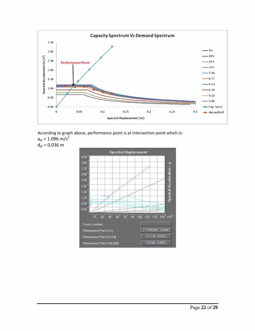
Page 22 of 29
According to graph above, performance point is at intersection point which is: api = 1.096 m/s2 dpi = 0.036 m
Page 23 of 29
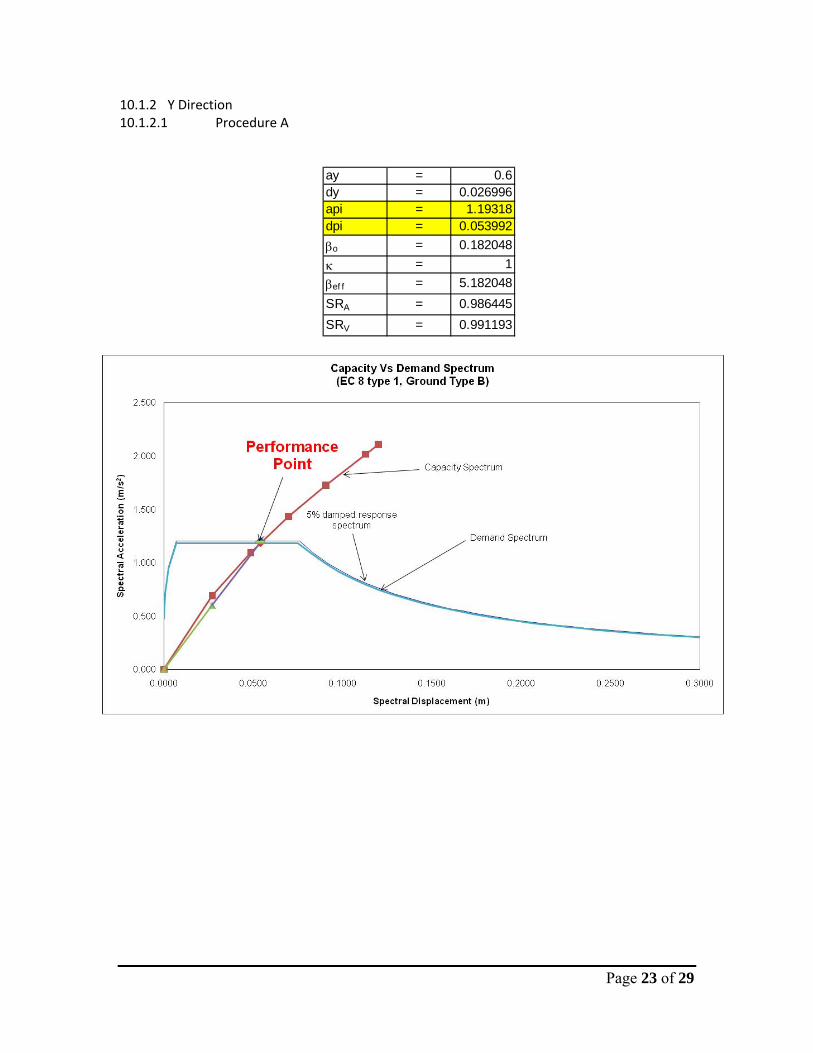
10.1.2 Y Direction 10.1.2.1 Procedure A
ay = 0.6dy = 0.026996api = 1.19318dpi = 0.053992βo = 0.182048κ = 1βef f = 5.182048SRA = 0.986445SRV = 0.991193
Page 24 of 29
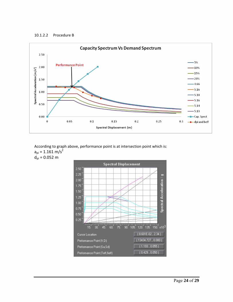
10.1.2.2 Procedure B
According to graph above, performance point is at intersection point which is: api = 1.161 m/s2 dpi = 0.052 m
Page 25 of 29
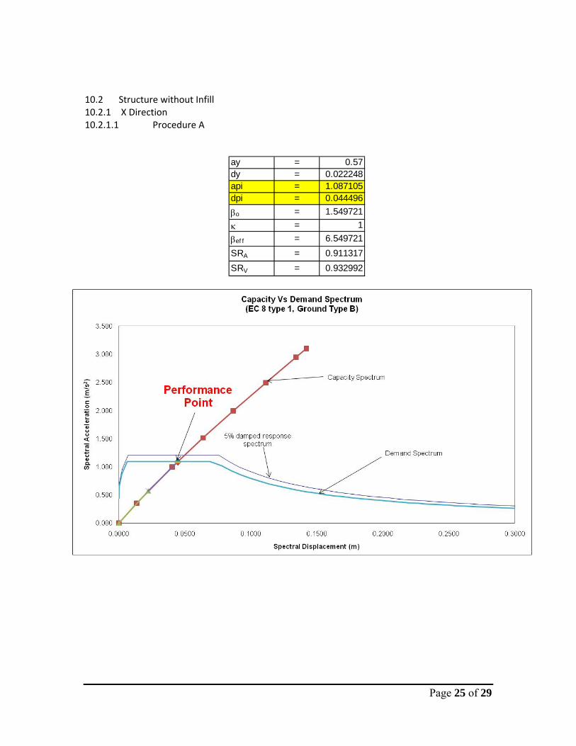
10.2 Structure without Infill 10.2.1 X Direction 10.2.1.1 Procedure A
ay = 0.57dy = 0.022248api = 1.087105dpi = 0.044496βo = 1.549721κ = 1βef f = 6.549721SRA = 0.911317SRV = 0.932992
Page 26 of 29
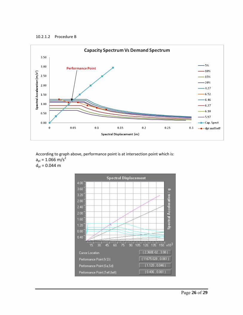
10.2.1.2 Procedure B
According to graph above, performance point is at intersection point which is: api = 1.066 m/s2 dpi = 0.044 m
Page 27 of 29
10.2.2 Y Direction
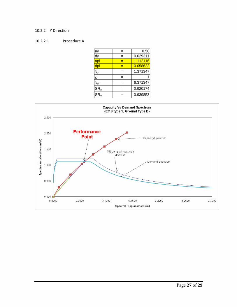
10.2.2.1 Procedure A
ay = 0.58dy = 0.029311api = 1.112116dpi = 0.058622βo = 1.371347κ = 1βef f = 6.371347SRA = 0.920174SRV = 0.939853
Page 28 of 29
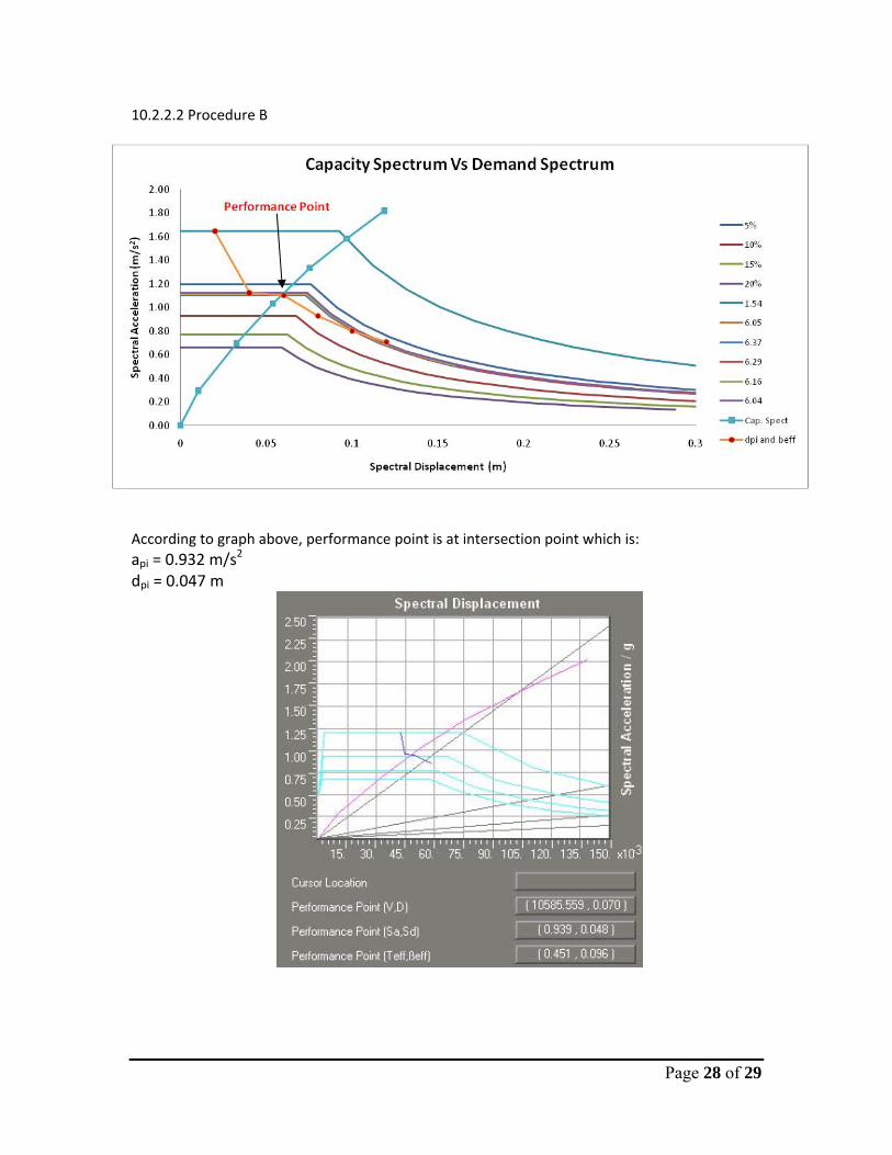
10.2.2.2 Procedure B
According to graph above, performance point is at intersection point which is: api = 0.932 m/s2 dpi = 0.047 m
Page 29 of 29
11. Conclusions
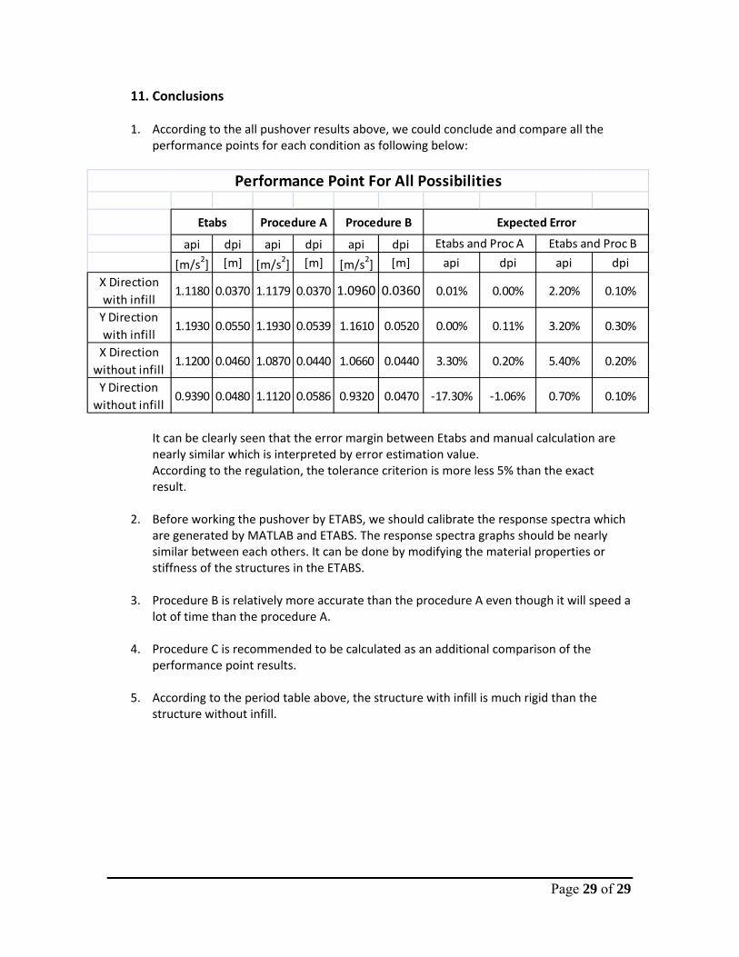
1. According to the all pushover results above, we could conclude and compare all the performance points for each condition as following below:
api dpi api dpi api dpi
[m/s2] [m] [m/s2] [m] [m/s2] [m] api dpi api dpi
X Direction with infill
1.1180 0.0370 1.1179 0.0370 1.0960 0.0360 0.01% 0.00% 2.20% 0.10%
Y Direction with infill
1.1930 0.0550 1.1930 0.0539 1.1610 0.0520 0.00% 0.11% 3.20% 0.30%
X Direction without infill
1.1200 0.0460 1.0870 0.0440 1.0660 0.0440 3.30% 0.20% 5.40% 0.20%
Y Direction without infill
0.9390 0.0480 1.1120 0.0586 0.9320 0.0470 ‐17.30% ‐1.06% 0.70% 0.10%
Performance Point For All Possibilities
Etabs Procedure A Procedure B
Etabs and Proc A Etabs and Proc B
Expected Error
It can be clearly seen that the error margin between Etabs and manual calculation are nearly similar which is interpreted by error estimation value. According to the regulation, the tolerance criterion is more less 5% than the exact result.
2. Before working the pushover by ETABS, we should calibrate the response spectra which are generated by MATLAB and ETABS. The response spectra graphs should be nearly similar between each others. It can be done by modifying the material properties or stiffness of the structures in the ETABS.
3. Procedure B is relatively more accurate than the procedure A even though it will speed a lot of time than the procedure A.
4. Procedure C is recommended to be calculated as an additional comparison of the performance point results.
5. According to the period table above, the structure with infill is much rigid than the structure without infill.