arX

iv:1

411.

2417

v2 [

cs.IT

] 7

Jan

2016

1

Capacity Results for Multicasting Nested MessageSets over Combination Networks

Shirin Saeedi Bidokhti, Vinod M. Prabhakaran, Suhas N. Diggavi

Abstract

The problem of multicasting two nested messages is studied over a class of networks known as combination networks. Asource multicasts two messages, a common and a private message, to several receivers. A subset of the receivers (called thepublic receivers) only demand the common message and the rest of the receivers (called the private receivers) demand boththe common and the private message. Three encoding schemes are discussed that employ linear superposition coding and theiroptimality is proved in special cases. The standard linear superposition scheme is shown to be optimal for networks withtwopublic receivers and any number of private receivers. When the number of public receivers increases, this scheme stops beingoptimal. Two improvements are discussed: one using pre-encoding at the source, and one using a block Markov encoding scheme.The rate-regions that are achieved by the two schemes are characterized in terms of feasibility problems. Both inner-bounds areshown to be the capacity region for networks with three (or fewer) public and any number of private receivers. Although the innerbounds are not comparable in general, it is shown through an example that the region achieved by the block Markov encodingscheme may strictly include the region achieved by the pre-encoding/linear superposition scheme. Optimality resultsare foundedon the general framework of Balister and Bollobas (2012) for sub-modularity of the entropy function. An equivalent graphicalrepresentation is introduced and a lemma is proved that might be of independent interest.

Motivated by the connections between combination networksand broadcast channels, a new block Markov encoding schemeis proposed for broadcast channels with two nested messages. The rate-region that is obtained includes the previously knownrate-regions. It remains open whether this inclusion is strict.

Index Terms

Network Coding, Combination Networks, Broadcast Channels, Superposition Coding, Linear Coding, Block Markov Encoding

I. I NTRODUCTION

The problem of communicating common and individual messages over general networks has been unresolved over the pastseveral decades, even in the two extreme cases of single-hopbroadcast channels and multi-hop wireline networks. Specialcases have been studied where the capacity region is fully characterized (see [1] and the references therein, and [2]–[5]).Inner and outer bounds on the capacity region are derived in [6]–[12]. Moreover, new encoding and decoding techniques aredeveloped such as superposition coding [13], [14], Marton’s coding [15]–[17], network coding [2], [18], [19], and joint uniqueand non-unique decoding [20]–[23].

Surprisingly, the problem of broadcasting nested (degraded) message sets has been completely resolved for two users. Theproblem was introduced and investigated for two-user broadcast channels in [17] and it was shown that superposition codingwas optimal. The problem has also been investigated for wired networks with two users [24]–[26] where a scheme consisting ofrouting and random network coding turns out to be rate-optimal. This might suggest that the nested structure of the messagesmakes the problem easier in nature. Unfortunately, however, the problem has remained open for networks with more thantwo receivers and only some special cases are understood [22], [27]–[30]. The state of the art is not favourable for wirednetworks either. Although extensions of the joint routing and network coding scheme in [24] are optimal for special classes ofthree-receiver networks (e.g., in [31]), they are suboptimal in general depending on the structure of the network [32, Chapter5], [33]. It was recently shown in [34] that the problem of multicasting two nested message sets over general wired networksis as hard as the general network coding problem.

In this paper, we study nested message set broadcasting overa class of wired networks known as combination networks[35]. These networks also form a resource-based model for broadcast channels and are a special class of linear deterministicbroadcast channels that were studied in [29], [30]. Lying atthe intersection of multi-hop wired networks and single-hopbroadcast channels, combination networks are an interesting class of networks to build up intuition and understanding, anddevelop new encoding schemes applicable to both sets of problems.

S. Saeedi Bidokhti was with the School of Computer and Communication Sciences, Ecole Polytechnique Federal de Lausanne. She is now with theDepartment of Electrical Engineering department for Communications Engineering, Technische Universitat Munchen(e-mail: shirin.saeedi@tum.de).

V. Prabhakaran is with the School of Technology and ComputerScience, Tata Institute of Fundamental Research (e-mail: vinodmp@tifr.res.in).S. Diggavi is with the Department of Electrical Engineering, UCLA, USA e-mail: (suhas@ee.ucla.edu).The work of S. Saeedi Bidokhti was partially supported by theSNSF fellowship no.146617. The work of Vinod M. Prabhakaranwas partially supported

by a Ramanujan Fellowship from the Department of Science andTechnology, Government of India. The work of S. Diggavi was supported in part by NSFawards 1314937 and 1321120.

The material in this paper was presented in parts at the 2009 IEEE Information Theory Workshop, Taormina, Italy, 2012 IEEE Information Theory Workshop,Lausanne, Switzerland, and the 2013 IEEE International Symposium on Information Theory, Istanbul, Turkey.

2

W1,W2

Encoder

Decoder1 Decoder2 Decoder3

W(2)1W

(1)1 W

(3)1 , W

(4)2

Y n1 =

Xn1

Xn3

Xn2

Y n2 =

[Xn

3

Xn2

]

Y n3 =

Xn1

Xn2

Xn4

Xn1 Xn

2Xn3 Xn

4

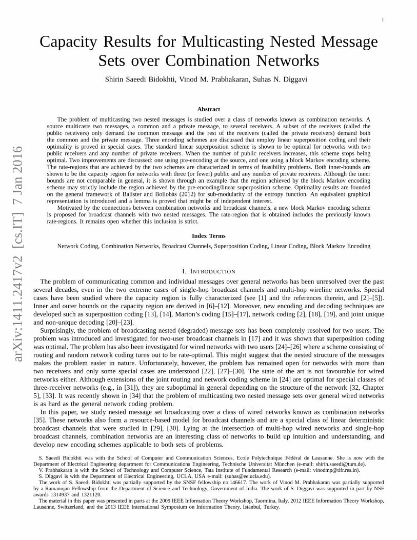
Fig. 1: A combination network with two public receivers indexed byI1 = {1, 2} and one private receiver indexed byI2 = {3}.All edges are of unit capacity.

We study the problem of multicasting two nested message sets(a common message and a private message) to multiple users.A subset of the users (public receivers) only demand the common message and the rest of the users (private receivers) demandboth the common message and the private message. The term private does not imply any security criteria in this paper.

Combination networks turn out to be an interesting class of networks that allow us to discuss new encoding schemes andobtain new capacity results. We discuss three encoding schemes and prove their optimality in several cases (depending on thenumber of public receivers, irrespective of the number of private receivers). In particular, we propose a block Markov encodingscheme that outperforms schemes based on rate splitting andlinear superposition coding. Our inner bounds are expressed interms of feasibility problems and are easy to calculate. To illustrate the implications of our approach over broadcast channels,we generlize our results and propose a block Markov encodingscheme for broadcasting two nested message sets over generalbroadcast channels (with multiple public and private receivers). The rate-region that is obtained includes previously knownrate-regions.

A. Communication Setup

A combination network is a three-layer directed network with one source and multiple destinations. It consists of a sourcenode in the first layer,d intermediate nodes in the second layer andK destination nodes in the third layer. The source isconnected to all intermediate nodes, and each intermediatenode is connected to a subset of the destinations. We refer totheoutgoing edges of the source as theresourcesof the combination network, see Fig. 1. We assume that each edge in this networkcarries one symbol from a finite fieldFq. We express all rates in symbols per channel use (log2 q bits per channel use) andthus all edges are of unit capacity.

The communication setup is shown in Fig. 1. A source multicasts a common messageW1 of nR1 bits and a private messageW2 of nR2 bits. W1 andW2 are independent. The common message is to be reliably decoded at all destinations, and theprivate message is to be reliably decoded at a subset of the destinations. We refer to those destinations who demand bothmessages asprivate receiversand to those who demand only the common message aspublic receivers. We denote the numberof public receivers bym and assume, without loss of generality, that they are indexed 1, . . . ,m. The set of all public receiversis denoted byI1 = {1, 2, . . . ,m} and the set of all private receivers is denoted byI2 = {m+ 1, . . . ,K}.

Encoding is done over blocks of lengthn. The encoderencodesW1 andW2 into d sequencesXni , i = 1, . . . , d, that are

sent over the resources of the combination network (overn uses of the network). Based on the structure of the network, eachuseri receives a vector of sequences,Y n

i , that is a certain collection of sequences that were sent by the source. GivenY ni ,

public receiveri, i = 1, . . . ,m, decodesW (i)1 and givenY n

p , private receiverp, p = m+ 1, . . . ,K, decodesW (p)1 , W

(p)2 . A

rate pair(R1, R2) is said to be achievable if there is an encoding/decoding scheme that allows the error probability

Pe = Pr(

W(i)1 6= W1 for somei = 1, . . . ,K or W (i)

2 6= W2 for somei = m+ 1, . . . ,K)

approach zero (asn → ∞). We call the closure of all achievable rate-pairs the capacity region. Although we allowǫ−errorprobability in the communication scheme (for example in proving converse theorems), the achievable schemes that we propose

3

S

W1 = [w1,1]

W2 = [w2,1, w2,2]

D1

W1

D2

W1, w2,1

D3

W1,W2

D4

W1,W2

w1,1w1,1 + w2,1 w2,1 w2,2

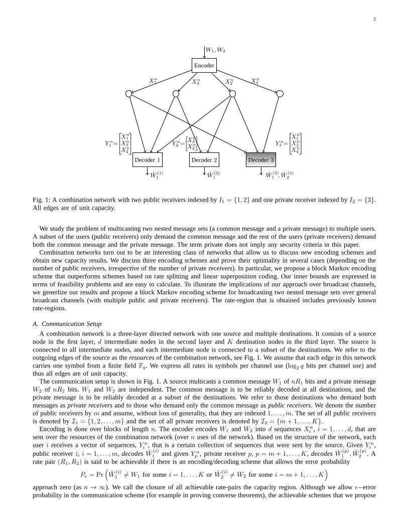
Fig. 2: The source multicastsW1 = [w1,1] andW2 = [w2,1, w2,2] (of ratesR1 = 1 andR2 = 2) in n = 1 channel use.

are zero-error schemes. Therefore, in all cases where we characterize the capacity region, theǫ−error capacity region and thezero-error capacity region coincide. This is not surprising considering the deterministic nature of our channels/networks.

B. Organization of the Paper

The paper is organized in eight sections. In Section II, we give an overview of the underlying challenges and our main ideasthrough several examples. Our notation is introduced in Section III. We study linear encoding schemes that are based on ratesplitting, linear superposition coding, and pre-encodingin Section IV. Section V proposes a block Markov encoding schemefor multicasting nested message sets, Section VI discussesoptimality results, and Section VII generalizes the block Markovencoding scheme of Section V to general broadcast channels.We conclude in Section VIII.

II. M AIN IDEAS AT A GLANCE

The problem of multicasting messages to receivers which have (two) different demands over a shared medium (such asthe combination network) is, in a sense, finding an optimal solution to a trade-off. On the one hand, public receivers (whichpresumably have access to fewer resources) need information about the common messageonly so that each can decodethe common message. On the other hand, private receivers require complete information of both messages. It is, therefore,desirable from private receivers’ point of view to have these messages jointly encoded (especially when there are multipleprivate receivers). This may be in contrast with public receivers’ decodability requirement. This tension is best seenthroughan example. Example 1 below shows that an optimal encoding scheme should allow joint encoding of the common and privatemessages but in a restricted and controlled manner, so that only partial information about the private message is “revealed”to the public receivers and decodability of the common message is ensured.

Example 1. Consider the combination network shown in Fig. 2 inn = 1 channel use. The source communicates a commonmessageW1 = [w1,1] and a private messageW2 = [w2,1, w2,2] to four receivers. Receivers1 and2 are public receivers andreceivers3 and4 are private receivers. Since Receivers1 and2 each have min-cuts less than3, they are not able to decodeboth the common and private messages. For this reason, random linear network coding does not ensure decodability ofW1

at the public receivers. We note that to communicateW1,W2, it is necessary that some partial information about the privatemessage is revealed to public receiver2.

Split the private message intow2,1 of rateα{2} = 1 andw2,2 of rateαφ = 1. w2,2 is the part ofW2 that is not revealed tothe public receivers andw2,1 is the part that is revealed to Receiver2 (but not Receiver1). By splitting W2 into independentpieces, we make sure that only a part ofW2, in this casew2,1, is revealed to Receiver2; In other words, onlyw2,1 is encodedinto sequencesXn

i ’s that are received by Receiver2. A linear scheme based on this idea is illustrated in Fig. 2 and could berepresented as follows:

X1

X2

X3

X4

=

1 1 01 0 00 1 00 0 1

w1,1

w2,1

w2,2

. (1)

4

S

W1 = []

W2 = [w2,1, w2,2]

D1 D2 D3 D4 D5 D6

X1 X2 X3

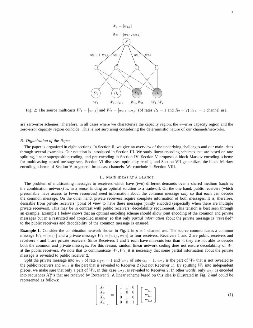
Fig. 3: MulticastingW1 of rate 0 andW2 of rate 2. A multicast code such asX1 = w2,1, X2 = w2,2, X3 = w2,1 + w2,2

ensures achievability of(R1 = 0, R2 = 2).

Note that by this construction we have ensured that the private receivers get a full rank transformation of all information symbols,and the public receivers get a full rank transformation of a subset of the information symbols (including the information symbolof W1). △

Our first coding scheme (Proposition 1 in Section IV-C) builds on Example 1 by splitting the private message into2m

independent pieces (of ratesαS , S ⊆ I, to be optimized) and using linear superposition coding. The rate split parametersαS

should be designed such that they satisfy several rank constraints (for different decoders to decode their messages of interest).We characterize the achievable rate-region by a linear program with no objective function (a feasibility problem). Thesolutionof this linear program gives the optimal choice ofαS for the scheme. We show that our scheme is optimal for combinationnetworks with two public and any number of private receivers.

For networks with three or more public and any number of private receivers, the above scheme may perform sub-optimally.It turns out that one may, depending on the structure of resources, gain by introducing dependency among the partial (private)information that is revealed to different subsets of publicreceivers.

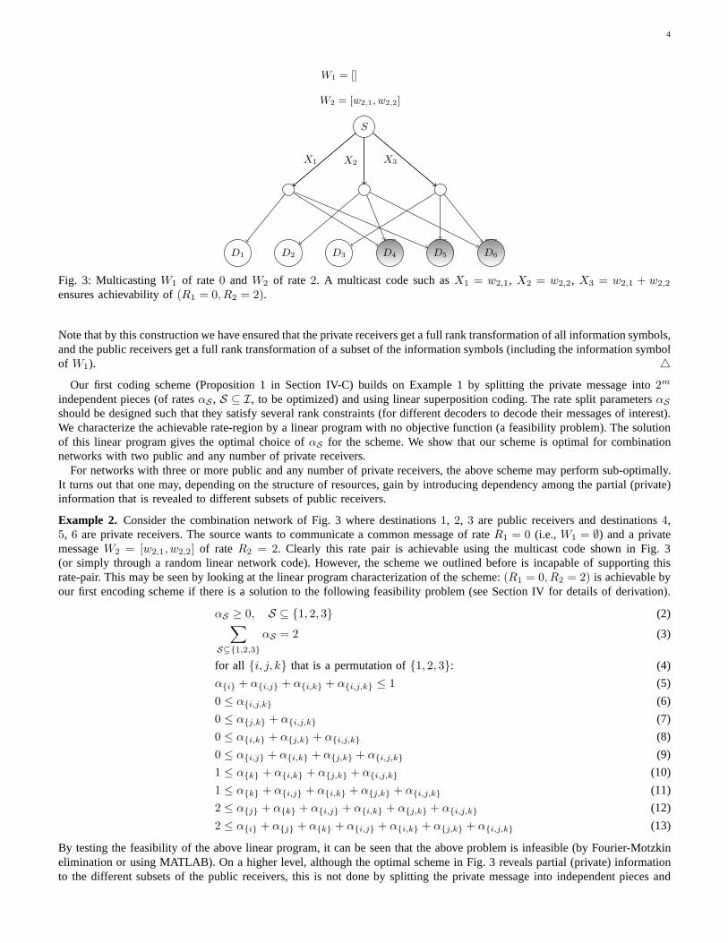
Example 2. Consider the combination network of Fig. 3 where destinations 1, 2, 3 are public receivers and destinations4,5, 6 are private receivers. The source wants to communicate a common message of rateR1 = 0 (i.e., W1 = ∅) and a privatemessageW2 = [w2,1, w2,2] of rate R2 = 2. Clearly this rate pair is achievable using the multicast code shown in Fig. 3(or simply through a random linear network code). However, the scheme we outlined before is incapable of supporting thisrate-pair. This may be seen by looking at the linear program characterization of the scheme:(R1 = 0, R2 = 2) is achievable byour first encoding scheme if there is a solution to the following feasibility problem (see Section IV for details of derivation).

αS ≥ 0, S ⊆ {1, 2, 3} (2)∑

S⊆{1,2,3}

αS = 2 (3)

for all {i, j, k} that is a permutation of{1, 2, 3}: (4)

α{i} + α{i,j} + α{i,k} + α{i,j,k} ≤ 1 (5)

0 ≤ α{i,j,k} (6)

0 ≤ α{j,k} + α{i,j,k} (7)

0 ≤ α{i,k} + α{j,k} + α{i,j,k} (8)

0 ≤ α{i,j} + α{i,k} + α{j,k} + α{i,j,k} (9)

1 ≤ α{k} + α{i,k} + α{j,k} + α{i,j,k} (10)

1 ≤ α{k} + α{i,j} + α{i,k} + α{j,k} + α{i,j,k} (11)

2 ≤ α{j} + α{k} + α{i,j} + α{i,k} + α{j,k} + α{i,j,k} (12)

2 ≤ α{i} + α{j} + α{k} + α{i,j} + α{i,k} + α{j,k} + α{i,j,k} (13)

By testing the feasibility of the above linear program, it can be seen that the above problem is infeasible (by Fourier-Motzkinelimination or using MATLAB). On a higher level, although the optimal scheme in Fig. 3 reveals partial (private) informationto the different subsets of the public receivers, this is notdone by splitting the private message into independent pieces and

5

there is a certain dependency structure between the symbolsthat are revealed to receivers1, 2, and3. This is why our firstlinear superposition scheme does not support the rate-pair(0, 2).

We use this observation to modify the encoding scheme and achieve the rate pair(0, 2). First, pre-encode messageW2,through a pre-encoding matrixP ∈ Fq

3×2, into a pseudo private messageW ′2 of larger “rate”:

w′2,1

w′2,2

w′2,3

= P

[

w′2,1w′2,2

]

. (14)

Then, encodeW ′2 using rate splitting and linear superposition coding:

X1

X2

X3

=

1 0 00 1 00 0 1

w′2,1

w′2,2

w′2,3

. (15)

SupposeP is a MDS (maximum distance separable) code. Each private receiver is able to decode two symbols out of thethree symbols ofW ′

2 and can thus decodeW2. It turns out that the achievable rate-region of this schemeis a relaxation of(2)-(13) whenαφ may be negative. △

Our second approach (Theorem 1 in Section IV-D) builds on Example 2 and the underlying idea is to allow dependencyamong the pieces of information that are revealed to different sets of public receivers by an appropriate pre-encoder that encodesthe private message into a pseudo private message of a largerrate, followed by a linear superposition encoding scheme. Weprove that the rate-region achieved by our second scheme is tight for m = 3 (or fewer) public receivers and any number ofprivate receivers. To prove the converse, we first write an outer-bound on the rate-region which lookssimilar to the inner-boundfeasibility problem and is in terms of some entropy functions. Next, we usesub-modularity of entropyto write a conversefor every inequality of the inner bound. In this process, we develop a visual tool in the framework of [36] to deal with thesub-modularity of entropy and prove a lemma that allows us show the tightness of the inner bound without explicitly solvingits corresponding feasibility problem.

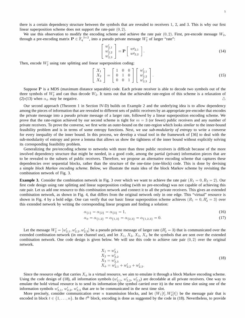
Generalizing the pre/encoding scheme to networks with morethan three public receivers is difficult because of the moreinvolved dependency structure that might be needed, in a good code, among the partial (private) information pieces thatareto be revealed to the subsets of public receivers. Therefore, we propose an alternative encoding scheme that captures thesedependencies over sequential blocks, rather than the structure of the one-time (one-block) code. This is done by devisinga simpleblock Markov encoding scheme. Below, we illustrate the main idea of the block Markov scheme by revisiting thecombination network of Fig. 3.

Example 3. Consider the combination network in Fig. 3 over which we wantto achieve the rate pair(R1 = 0, R2 = 2). Ourfirst code design using rate splitting and linear superposition coding (with no pre-encoding) was not capable of achieving thisrate pair. Let us add one resource to this combination network and connect it to all the private receivers. This gives an extendedcombination network, as shown in Fig. 4, that differs from the original network only in one edge. This “virtual” resourceisshown in Fig. 4 by a bold edge. One can verify that our basic linear superposition scheme achieves(R1 = 0, R′

2 = 3) overthis extended network by writing the corresponding linear program and finding a solution:

α{1} = α{2} = α{3} = 1, (16)

αφ = α{1,2} = α{1,3} = α{2,3} = α{1,2,3} = 0. (17)

Let the messageW ′2 = [w′

2,1, w′2,2, w

′2,3] be a pseudo private message of larger rate (R′

2 = 3) that is communicated over theextended combination network (in one channel use), and letX1, X2, X3, Xφ be the symbols that are sent over the extendedcombination network. One code design is given below. We willuse this code to achieve rate pair(0, 2) over the originalnetwork.

X1 = w′2,1

X2 = w′2,2

X3 = w′2,3

Xφ = w′2,1 + w′

2,2 + w′2,3.

(18)

Since the resource edge that carriesXφ is a virtual resource, we aim to emulate it through a block Markov encoding scheme.Using the code design of (18), all information symbols (w′

2,1, w′2,2, w′

2,3) are decodable at all private receivers. One way toemulate the bold virtual resource is to send its information(the symbol carried over it) in the next time slot using one oftheinformation symbolsw′

2,1, w′2,2, w′

2,3 that are to be communicated in the next time slot.More precisely, consider communication overn transmission blocks, and let(W1[t],W

′2[t]) be the message pair that is

encoded in blockt ∈ {1, . . . , n}. In the tth block, encoding is done as suggested by the code in (18). Nevertheless, to provide

6

S

W1[t+ 1] = []

W ′2[t+ 1] = [w′

2,1[t+ 1], w′2,2[t+ 1], w′

2,3[t+ 1]]

D1 D2 D3 D4 D5 D6

X1[t] X2[t] X3[t] Xφ[t]

Fig. 4: The extended combination network of Example 3. A block Markov encoding scheme achieves(0, 2) over the originalcombination network. At timet+ 1, information symbolw′

2,3[t+ 1] contains the information of symbolXφ[t].

private receivers with the information ofXφ[t] (as promised by the virtual resource), we usew′2,3[t + 1] in the next block

to conveyXφ[t]. Since this symbol is ensured to be decoded at the private receivers, it indeed emulates the virtual resource.In the nth block, we simply encodeXφ[n− 1] and directly communicate it with the private receivers. Upon receiving all then blocks at the receivers, we perform backward decoding [37].So in n transmissions, we sendn − 1 symbols ofW1 and2(n− 1)+1 new symbols ofW2 over the original combination network; i.e., forn→∞, we achieve the rate-pair(0, 2). △

Out third coding scheme (Theorem 2 in Section V) builds on Example 3. When there arem = 4 or more public receivers,our block Markov scheme is more powerful that the first two schemes and we are not aware of any example where this schemeis sub-optimal. In Section V, we describe our block Markov encoding scheme and characterize the rate region it achieves.We show, for three (or fewer) public and any number of privatereceivers, that this rate-region is equal to the capacity regionand, therefore, coincides with the rate-region of Theorem 1. Furthermore, we show through an example that the block Markovencoding scheme could outperform the previously discussedlinear encoding schemes when there are4 or more public receivers.

In Section VII, we further adapt this scheme to general broadcast channels with two nested message sets and obtain a rateregion that includes previously known rate-regions. We do not know if this inclusion is strict.

III. NOTATION

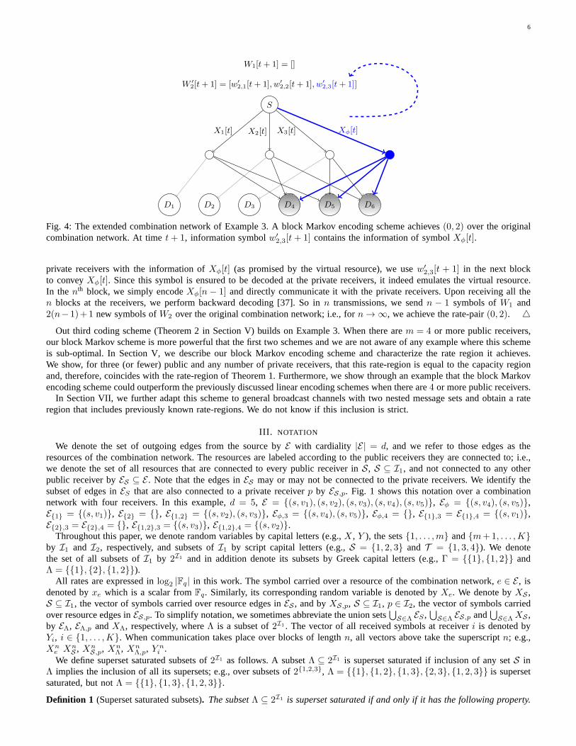
We denote the set of outgoing edges from the source byE with cardiality |E| = d, and we refer to those edges as theresources of the combination network. The resources are labeled according to the public receivers they are connected to; i.e.,we denote the set of all resources that are connected to everypublic receiver inS, S ⊆ I1, and not connected to any otherpublic receiver byES ⊆ E . Note that the edges inES may or may not be connected to the private receivers. We identify thesubset of edges inES that are also connected to a private receiverp by ES,p. Fig. 1 shows this notation over a combinationnetwork with four receivers. In this example,d = 5, E = {(s, v1), (s, v2), (s, v3), (s, v4), (s, v5)}, Eφ = {(s, v4), (s, v5)},E{1} = {(s, v1)}, E{2} = {}, E{1,2} = {(s, v2), (s, v3)}, Eφ,3 = {(s, v4), (s, v5)}, Eφ,4 = {}, E{1},3 = E{1},4 = {(s, v1)},E{2},3 = E{2},4 = {}, E{1,2},3 = {(s, v3)}, E{1,2},4 = {(s, v2)}.

Throughout this paper, we denote random variables by capital letters (e.g.,X , Y ), the sets{1, . . . ,m} and{m+1, . . . ,K}by I1 and I2, respectively, and subsets ofI1 by script capital letters (e.g.,S = {1, 2, 3} and T = {1, 3, 4}). We denotethe set of all subsets ofI1 by 2I1 and in addition denote its subsets by Greek capital letters (e.g.,Γ = {{1}, {1, 2}} andΛ = {{1}, {2}, {1, 2}}).

All rates are expressed inlog2 |Fq| in this work. The symbol carried over a resource of the combination network,e ∈ E , isdenoted byxe which is a scalar fromFq. Similarly, its corresponding random variable is denoted by Xe. We denote byXS ,S ⊆ I1, the vector of symbols carried over resource edges inES , and byXS,p, S ⊆ I1, p ∈ I2, the vector of symbols carriedover resource edges inES,p. To simplify notation, we sometimes abbreviate the union sets

⋃

S∈Λ ES ,⋃

S∈Λ ES,p and⋃

S∈ΛXS ,by EΛ, EΛ,p andXΛ, respectively, whereΛ is a subset of2I1 . The vector of all received symbols at receiveri is denoted byYi, i ∈ {1, . . . ,K}. When communication takes place over blocks of lengthn, all vectors above take the superscriptn; e.g.,Xn

e XnS , Xn

S,p, XnΛ, Xn

Λ,p, Y ni .

We define superset saturated subsets of2I1 as follows. A subsetΛ ⊆ 2I1 is superset saturated if inclusion of any setS inΛ implies the inclusion of all its supersets; e.g., over subsets of 2{1,2,3}, Λ = {{1}, {1, 2}, {1, 3}, {2, 3}, {1, 2, 3}} is supersetsaturated, but notΛ = {{1}, {1, 3}, {1, 2, 3}}.

Definition 1 (Superset saturated subsets). The subsetΛ ⊆ 2I1 is superset saturated if and only if it has the following property.

7

S

v1 v2 v3 v4 v5

D1 D2 D3 D4

E{1} E{1,2},3

E{1,2} E{φ}

Fig. 5: A combination network with two public receivers indexed by I1 = {1, 2} and two private receivers indexed byI2 = {3, 4}.

• S is an element ofΛ only if everyT ∈ 2I1, T ⊇ S, is an element ofΛ.

For notational matters, we sometimes abbreviate a supersetsaturated subsetΛ by the few sets that are not implied by the othersets inΛ. For example,{{1}, {1, 2}, {1, 3}, {1, 2, 3}} is denoted by{{1}⋆}, and similarly{{1}, {1, 2}, {1, 3}, {2, 3}, {1, 2, 3}}is denoted by{{1}⋆, {2, 3}⋆}.

IV. RATE SPLITTING AND L INEAR ENCODING SCHEMES

Throughout this section, we confine ourselves to linear encoding at the source. For simplicity, we describe our encodingschemes for block lengthn = 1, and highlight cases where we need to code over longer blocks.

We assume ratesR1 andR2 to be non-negative integer values1. Let w1,1, . . . , w1,R1andw2,1, . . . , w2,R2

be variables inFq

for messagesW1 andW2, respectively. We call them the information symbols of the common and the private message. Also,let vectorW ∈ Fq

R1+R2 be defined as the vector with coordinates in the standard basis W = [w1,1 . . . w1,R2w2,1 . . . w2,R2

]T .The symbol carried by each resource is a linear combination of the information symbols. After properly rearranging all vectorsXS , S ⊆ I1, we have

X{1,...,m}

...X{2}

X{1}

Xφ

= A ·W,

whereA ∈ Fqd×(R1+R2) is the encoding matrix. At each public receiveri, i ∈ I1, the received signalYi is given byYi = AiW ,

whereAi is a submatrix ofA corresponding toXS , S ∋ i. Similarly, the received signal at each private receiverp, p ∈ I2,is given byYp = ApW , whereAp is the submatrix of the rows ofA corresponding toXS,p, S ⊆ I1.

We designA to allow the public receivers decodeW1 and the private receivers decodeW1,W2. We then characterize therate pairs achievable by our code design. The challenge in the optimal code design stems from the fact that destinations receivedifferent subsets of the symbols that are sent by the encoderand they have two different decodability requirements. On theone hand, private receivers require their received signal to bring information about all information symbols of the common andthe private message. On the other hand, public receivers might not be able to decode the common message if their receivedsymbols depend on “too many” private message variables. We make this statement precise in Lemma 1. In the following, wefind conditions for decodability of the messages.

A. Decodability Lemmas

Lemma 1. Let vectorY be given by(19), below, whereB ∈ Fqr×R1 , T ∈ Fq

r×R2 , W1 ∈ FqR1×1, andW2 ∈ Fq

R2×1.

Y =[

B T]

·

[

W1

W2

]

. (19)

MessageW1 is recoverable fromY if and only if rank(B) = R1 and the column space ofB is disjoint from that ofT.

1There is no loss of generality in this assumption. One can deal with rational values ofR1 andR2 by coding over blocks of large enough lengthn andworking with integer ratesnR1 andnR2. Also, one can attain real valued rates through sequences ofrational numbers that approach them.

8

Corollary 1. MessageW1 is recoverable fromY in equation(19) only if

rank(T) ≤ r −R1.

We defer the proof of Lemma 1 to Appendix A and instead discussthe high-level implication of the result. LetrT = rank(T)whererT ≤ r − R1. Matrix T can be written asL1L2, whereL1 is a full-rank matrix of dimensionr × rT andL2 is afull-rank matrix of dimensionrT ×R2. L1 is essentially just a set of linearly independent columns ofT spanning its columnspace. In other words, we can write

[

B T]

W =[

B L1L2

]

W (20)

=[

B L1

]

[

W1

L2W2

]

. (21)

SincerT +R1 ≤ r, W1,L2W2 are decodable if[

B L1

]

is full-rank.Defining

[

B T]

as a newB′ of dimensionr × (R1 +R2) and defining a null matrixT′ in Lemma 1, we reach at thetrivial result of the following corollary.

Corollary 2. MessagesW1,W2 are recoverable fromY in equation(19) if and only if

rank([

B T])

= R1 +R2.

Since every receiver sees a different subset of the sent symbols, it becomes clear from Corollary 1 and 2 that an admissiblelinear code needs to satisfy many rank constraints on its different submatrices. In this section, our primary approach to thedesign of such codes is through zero-structured matrices, discussed next.

B. Zero-structured matrices

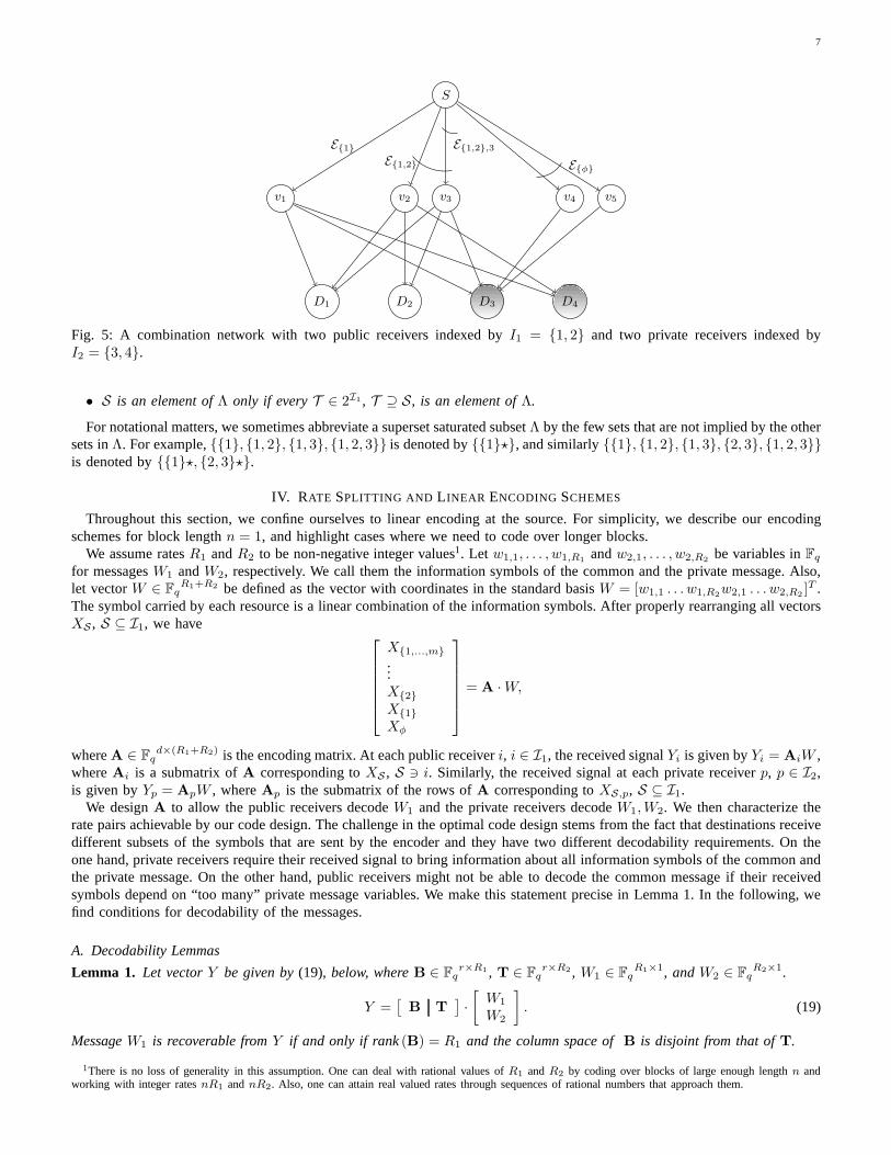
Definition 2. A zero-structured matrixT is anr× c matrix with entries either zero or indeterminate2 (from a finite fieldFq) ina specific structure, as follows. This matrix consists of2t×2t blocks, where each block is indexed on rows and columns by thesubsets of{1, · · · , t}. Block b(S1,S2), S1,S2 ⊆ {1, · · · , t}, is an rS1

× cS2matrix. Matrix T is structured so that all entries

in block b(S1,S2) are set to zero ifS1 6⊆ S2, and remain indeterminate otherwise. Note thatc =∑

S cS and r =∑

S rS .

Equation (22), below, demonstrates this definition fort = 2.

T =

c{1,2}←→

c{1}↔

c{2}↔

cφ↔

0 0 00 0

0 0

llll

r{1,2}

r{1}

r{2}

rφ

(22)

The idea behind using zero-structred encoding matrices is the following: the zeros are inserted in the encoding matrix suchthat the linear combinations that are formed for the public receivers do not depend on “too many” private information symbols(see Corollary 1).

In the rest of this subsection, we find conditions on zero-structured matrices so that they can be made full column rank.

Lemma 2. There exists an assignment of the indeterminates in the zero-structured matrixT ∈ Fqr×c (as specified in

Definition 2) that makes it full column rank, provided that

c ≤∑

S∈Λ

cS +∑

S∈Λc

rS , ∀Λ ⊆ 2{1,...,t} superset saturated. (23)

For t = 2, (23) is given by

c ≤ r{1,2} + r{1} + r{2} + rφ (24)

c ≤ c{1,2} + r{1} + r{2} + rφ (25)

c ≤ c{1} + c{1,2} + r{2} + rφ (26)

c ≤ c{2} + c{1,2} + r{1} + rφ (27)

c ≤ c{1} + c{2} + c{1,2} + rφ (28)

c ≤ cφ + c{1} + c{2} + c{1,2}. (29)

We briefly outline the proof of Lemma 2, because this line of argument is used later in Section IV-D. For simplicity ofnotation and clarity of the proof, we give details of the proof for t = 2. The same proof technique proves the general case.

2Although zero-structured matrices are defined in Definition2 with zero or indeterminate variables, we also refer to the assignments of such matrices aszero-structured matrices.

9

A

source

n{1,2} n{2} n{1}nφ

n′{1,2} n′

{2} n′{1} n′

φ

Bsink

c{1,2} c{2} c{1} cφ

r{1,2} r{2} r{1} rφ

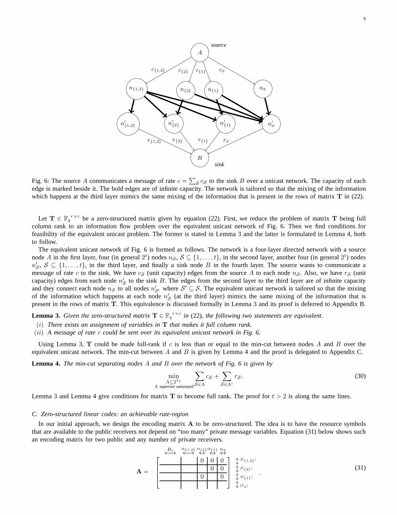
Fig. 6: The sourceA communicates a message of ratec =∑

S cS to the sinkB over a unicast network. The capacity of eachedge is marked beside it. The bold edges are of infinite capacity. The network is tailored so that the mixing of the informationwhich happens at the third layer mimics the same mixing of theinformation that is present in the rows of matrixT in (22).

Let T ∈ Fqr×c be a zero-structured matrix given by equation (22). First, we reduce the problem of matrixT being full

column rank to an information flow problem over the equivalent unicast network of Fig. 6. Then we find conditions forfeasibility of the equivalent unicast problem. The former is stated in Lemma 3 and the latter is formulated in Lemma 4, bothto follow.

The equivalent unicast network of Fig. 6 is formed as follows. The network is a four-layer directed network with a sourcenodeA in the first layer, four (in general2t) nodesnS , S ⊆ {1, . . . , t}, in the second layer, another four (in general2t) nodesn′S , S ⊆ {1, . . . , t}, in the third layer, and finally a sink nodeB in the fourth layer. The source wants to communicate a

message of ratec to the sink. We havecS (unit capacity) edges from the sourceA to each nodenS . Also, we haverS (unitcapacity) edges from each noden′

S to the sinkB. The edges from the second layer to the third layer are of infinite capacityand they connect each nodenS to all nodesn′

S′ whereS ′ ⊆ S. The equivalent unicast network is tailored so that the mixingof the information which happens at each noden′

S (at the third layer) mimics the same mixing of the information that ispresent in the rows of matrixT. This equivalence is discussed formally in Lemma 3 and its proof is deferred to Appendix B.

Lemma 3. Given the zero-structured matrixT ∈ Fqr×c in (22), the following two statements are equivalent.

(i) There exists an assignment of variables inT that makes it full column rank.(ii) A message of ratec could be sent over its equivalent unicast network in Fig. 6.

Using Lemma 3,T could be made full-rank ifc is less than or equal to the min-cut between nodesA andB over theequivalent unicast network. The min-cut betweenA andB is given by Lemma 4 and the proof is delegated to Appendix C.

Lemma 4. The min-cut separating nodesA andB over the network of Fig. 6 is given by

minΛ⊆2I1

Λ superset saturated

∑

S∈Λ

cS +∑

S∈Λc

rS . (30)

Lemma 3 and Lemma 4 give conditions for matrixT to become full rank. The proof fort > 2 is along the same lines.

C. Zero-structured linear codes: an achievable rate-region

In our initial approach, we design the encoding matrixA to be zero-structured. The idea is to have the resource symbolsthat are available to the public receivers not depend on “toomany” private message variables. Equation (31) below showssuchan encoding matrix for two public and any number of private receivers.

A =

R1←→α{1,2}←→

α{2}↔

α{1}↔

αφ

↔

0 0 00 0

0 0

llll

|E{1,2}|

|E{2}|

|E{1}|

|Eφ|

.(31)

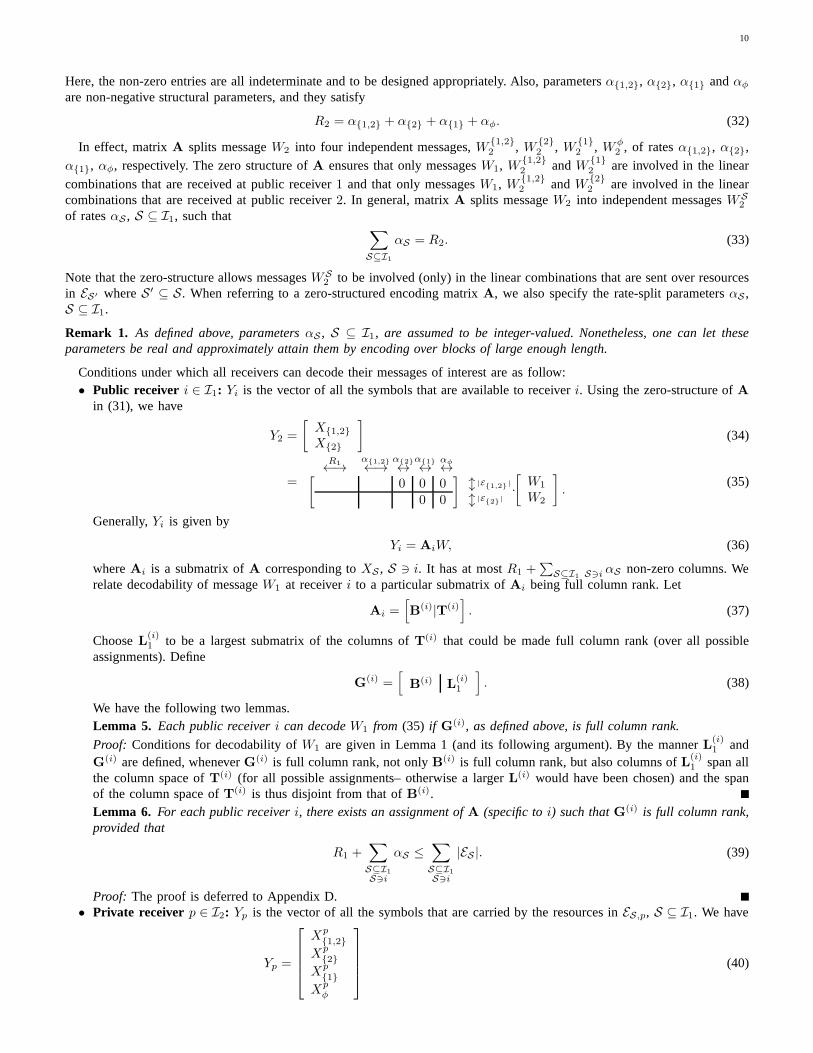
10

Here, the non-zero entries are all indeterminate and to be designed appropriately. Also, parametersα{1,2}, α{2}, α{1} andαφ

are non-negative structural parameters, and they satisfy

R2 = α{1,2} + α{2} + α{1} + αφ. (32)

In effect, matrixA splits messageW2 into four independent messages,W{1,2}2 , W {2}

2 , W {1}2 , Wφ

2 , of ratesα{1,2}, α{2},

α{1}, αφ, respectively. The zero structure ofA ensures that only messagesW1, W {1,2}2 andW {1}

2 are involved in the linear

combinations that are received at public receiver1 and that only messagesW1, W {1,2}2 andW {2}

2 are involved in the linearcombinations that are received at public receiver2. In general, matrixA splits messageW2 into independent messagesWS

2

of ratesαS , S ⊆ I1, such that∑

S⊆I1

αS = R2. (33)

Note that the zero-structure allows messagesWS2 to be involved (only) in the linear combinations that are sent over resources

in ES′ whereS ′ ⊆ S. When referring to a zero-structured encoding matrixA, we also specify the rate-split parametersαS ,S ⊆ I1.

Remark 1. As defined above, parametersαS , S ⊆ I1, are assumed to be integer-valued. Nonetheless, one can lettheseparameters be real and approximately attain them by encoding over blocks of large enough length.

Conditions under which all receivers can decode their messages of interest are as follow:• Public receiver i ∈ I1: Yi is the vector of all the symbols that are available to receiver i. Using the zero-structure ofA

in (31), we have

Y2 =

[

X{1,2}

X{2}

]

(34)

=

R1←→α{1,2}←→

α{2}↔

α{1}↔

αφ

↔[

0 0 00 0

]

ll

|E{1,2}|

|E{2}|·

[

W1

W2

]

.(35)

Generally,Yi is given by

Yi = AiW, (36)

whereAi is a submatrix ofA corresponding toXS , S ∋ i. It has at mostR1 +∑

S⊆I1 S∋i αS non-zero columns. Werelate decodability of messageW1 at receiveri to a particular submatrix ofAi being full column rank. Let

Ai =[

B(i)|T(i)

]

. (37)

ChooseL(i)1 to be a largest submatrix of the columns ofT

(i) that could be made full column rank (over all possibleassignments). Define

G(i) =

[

B(i)

L(i)1

]

. (38)

We have the following two lemmas.Lemma 5. Each public receiveri can decodeW1 from (35) if G(i), as defined above, is full column rank.

Proof: Conditions for decodability ofW1 are given in Lemma 1 (and its following argument). By the manner L(i)1 and

G(i) are defined, wheneverG(i) is full column rank, not onlyB(i) is full column rank, but also columns ofL(i)

1 span allthe column space ofT(i) (for all possible assignments– otherwise a largerL

(i) would have been chosen) and the spanof the column space ofT(i) is thus disjoint from that ofB(i).Lemma 6. For each public receiveri, there exists an assignment ofA (specific toi) such thatG(i) is full column rank,provided that

R1 +∑

S⊆I1

S∋i

αS ≤∑

S⊆I1

S∋i

|ES |. (39)

Proof: The proof is deferred to Appendix D.• Private receiver p ∈ I2: Yp is the vector of all the symbols that are carried by the resources inES,p, S ⊆ I1. We have

Yp =

Xp

{1,2}

Xp

{2}

Xp

{1}

Xpφ

(40)

11

=

R1←→α{1,2}←→

α{2}↔

α{1}↔

αφ

↔

0 0 00 0

0 0

llll

|E{1,2},p|

|E{2},p|

|E{1},p|

|Eφ,p|

·

[

W1

W2

]

.(41)

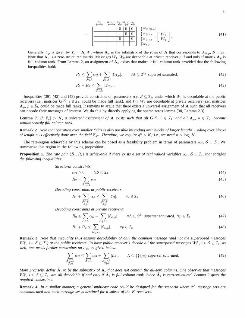
Generally,Yp is given byYp = ApW , whereAp is the submatrix of the rows ofA that corresponds toXS,p, S ⊆ I1.Note thatAp is a zero-structured matrix. MessagesW1,W2 are decodable at private receiverp if and only if matrixAp isfull column rank. From Lemma 2, an assignment ofAp exists that makes it full column rank provided that the followinginequalities hold:

R2 ≤∑

S∈Λ

αS +∑

S∈Λc

|ES,p|, ∀Λ ⊆ 2I1 superset saturated, (42)

R1 + R2 ≤∑

S⊆I1

|ES,p|. (43)

Inequalities (39), (42) and (43) provide constraints on parametersαS , S ⊆ I1, under whichW1 is decodable at the publicreceivers (i.e., matricesG(i), i ∈ I1, could be made full rank), andW1,W2 are decodable at private receivers (i.e., matricesAp, p ∈ I2, could be made full rank). It remains to argue that there exists a universal assignment ofA such that all receiverscan decode their messages of interest. We do this by directlyapplying the sparse zeros lemma [38, Lemma 2.3].

Lemma 7. If |Fq| > K, a universal assignment ofA exists such that allG(i), i ∈ I1, and all Ap, p ∈ I2, becomesimultaneously full column rank.

Remark 2. Note that operation over smaller fields is also possible by coding over blocks of larger lengths. Coding over blocksof lengthn is effectively done over the fieldFqn . Therefore, we requireqn > K; i.e., we needn > logq K.

The rate-region achievable by this scheme can be posed as a feasibility problem in terms of parametersαS , S ⊆ I1. Wesummarize this region in the following proposition.

Proposition 1. The rate pair(R1, R2) is achievable if there exists a set of real valued variablesαS , S ⊆ I1, that satisfiesthe following inequalities:

Structural constraints:

αS ≥ 0, ∀S ⊆ I1 (44)

R2 =∑

S⊆I1

αS (45)

Decoding constraints at public receivers:

R1 +∑

S⊆I1

S∋i

αS ≤∑

S⊆I1

S∋i

|ES |, ∀i ∈ I1 (46)

Decoding constraints at private receivers:

R2 ≤∑

S∈Λ

αS +∑

S∈Λc

|ES,p|, ∀Λ ⊆ 2I1 superset saturated, ∀p ∈ I2 (47)

R1 +R2 ≤∑

S⊆I1

|ES,p|, ∀p ∈ I2. (48)

Remark 3. Note that inequality(46) ensures decodability of only the common message (and not thesuperposed messagesWS

2 , i ∈ S ⊆ I1) at the public receivers. To have public receiveri decode all the superposed messagesWS2 , i ∈ S ⊆ I1, as

well, one needs further constraints onαS , as given below:∑

S⊆I1

S∋i

αS ≤∑

S∈Λ

αS +∑

S∈Λc

S∋i

|ES |, Λ ⊆ {{i}⋆} superset saturated. (49)

More precisely, defineAi to be the submatrix ofAi that does not contain the all-zero columns. One observes that messagesWS

2 , i ∈ S ⊆ I1, are all decodable if and only ifAi is full column rank. SinceAi is zero-structured, Lemma 2 gives therequired constraints.

Remark 4. In a similar manner, a general multicast code could be designed for the scenario where2K message sets arecommunicated and each message set is destined for a subset oftheK receivers.

12

Remark 5. What the zero-structure encoding matrix does, in effect, isimplement the standard techniques of rate splitting andlinear superposition coding. We prove in Subsection VI-A that this encoding scheme is rate-optimal for combination networkswith two public and any number of private receivers. However, this encoding scheme is not in general optimal. We discussthis sub-optimality next and modify the encoding scheme to attain a strictly larger rate region.

D. An achievable rate-region from pre-encoding and structured linear codes

For combination networks with three or more public receivers (and any number of private receivers), the scheme outlinedabove turns out to be sub-optimal in general. We discussed one such example in Example 2 where(R1 = 0, R2 = 2) wasnot achievable by Proposition 1 (see (2)-(13)). If we were torelax the non-negativity condition onαφ in (2)-(13), we wouldget feasibility of (R1, R2) = (0, 2) for the following set of parametersαS : αφ = −1, α{1} = α{2} = α{3} = 1, andα{1,2} = α{1,3} = α{2,3} = α{1,2,3} = 0. Obviously, there is no longer a “structural” meaning to this set of parameters.Nonetheless, it still has a peculiar meaning that we try to investigate in this example. As suggested by the positive parametersα{1}, α{2}, α{3}, we would like, in an optimal code design, to reveal a subspace of dimension one of the private message spaceto each public receiver (and only that public receiver). Thesubtlety lies in the fact that those pieces of private information arenot mutually independent, as messageW2 is of rate2. The previous scheme does not allow such dependency.

Inspired by Example 2, we modify the encoding scheme, using an appropriate pre-encoder, to obtain a strictly largerachievable region as expressed in Theorem 1.

Theorem 1. The rate pair(R1, R2) is achievable if there exists a set of real valued variablesαS , S ⊆ I1, that satisfy thefollowing inequalities:

Structural constraints:

αS ≥ 0, ∀S ⊆ I1, S 6= φ (50)

R2 =∑

S⊆I1

αS , (51)

Decoding constraints at public receivers:

R1 +∑

S⊆I1

S∋i

αS ≤∑

S⊆I1

S∋i

|ES |, ∀i ∈ I1 (52)

Decoding constraints at private receivers:

R2 ≤∑

S∈Λ

αS +∑

S∈Λc

|ES,p|, ∀Λ ⊆ 2I1 superset saturated, ∀p ∈ I2 (53)

R1 +R2 ≤∑

S⊆I1

|ES,p|, ∀p ∈ I2. (54)

Remark 6. Note that compared to Proposition 1, the non-negativity constraint onαφ is relaxed in Theorem 1.

Remark 7. The inner-bound of Theorem 1 is tight for combination networks withm = 3 (or fewer) public and any numberof private receivers, see Section VI-B.

Proof. Let (R1, R2) be in the rate region of Theorem 1; i.e., there exist parameters αS , S ⊆ I1, that satisfy inequalities(50)-(54). In the following, let(αφ)

− = min(0, αφ) and (αφ)+ = max(0, αφ). Furthermore, without loss of generality, we

assume that parametersR1, R2, αS , S ⊆ I1, are integer valued (see Remark 1).First of all, pre-encode messageW2 into a message vectorW ′

2 of dimensionR2 − (αφ)− through a pre-encoding matrix

P ∈ Fq[R2−(αφ)

−]×R2 ; i.e., we have

W ′2 = PW2. (55)

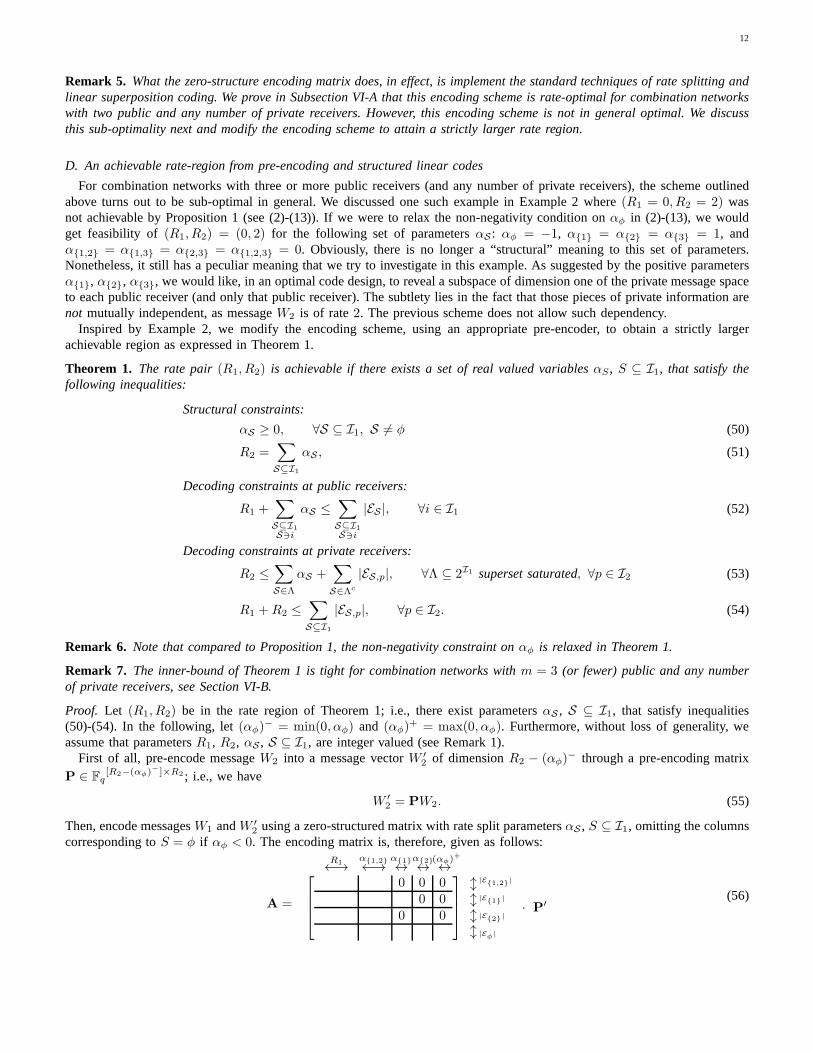
Then, encode messagesW1 andW ′2 using a zero-structured matrix with rate split parametersαS , S ⊆ I1, omitting the columns

corresponding toS = φ if αφ < 0. The encoding matrix is, therefore, given as follows:

A =

R1←→α{1,2}←→

α{1}↔

α{2}↔

(αφ)+

↔

0 0 00 0

0 0

llll

|E{1,2}|

|E{1}|

|E{2}|

|Eφ|

· P′(56)

13

where

P′ =

IR1×R10

0 P

, (57)

and all indeterminates are to be assigned from the finite fieldFq.The conditions for decodability ofW1 at each public receiveri ∈ I1 are given by (52), and the conditions for decodability

of W1,W2 at each private receiverp ∈ I2 is given by (53), (54). The proof is similar to the basic zero structured encodingscheme and is sketched in the following.

Let Ai be the submatrix ofA that constitutesYi at receiveri. We have

Ai =[

B(i)|T(i)

]

P′ (58)

=[

B(i)|T(i)

P

]

. (59)

As before, defineL(i)1 to be a largest submatrix of the columns ofT

(i)P that could be made full column rank (over all possible

assignments). DefineG(i) to be

G(i) =

[

B(i)|L(i)

1

]

. (60)

From Lemma 5, each receiveri can decodeW1 from (35) if G(i), as defined above, is full column rank. This is possibleprovided that (see Lemma 6)

R1 +∑

S⊆I1

S∋i

αS ≤∑

S⊆I1

S∋i

|ES |. (61)

Decodability ofW1 at private receiverp ∈ I2 is similarly guaranteed by (54). Finally,T(p)P could itself be full rank under

(53), see Appendix E, and thereforeW2 is decodable at private receivers (in addition toW1). Since the variables involved inB

(p) andT(p)P are independent,G(p) could be made full column rank.

It remains to argue that for|Fq| > K, and under (52)-(54), all matricesG(i), i ∈ I, could be made full rank simultaneously.The proof is based on the sparse zeros lemma and is deferred toAppendix F.

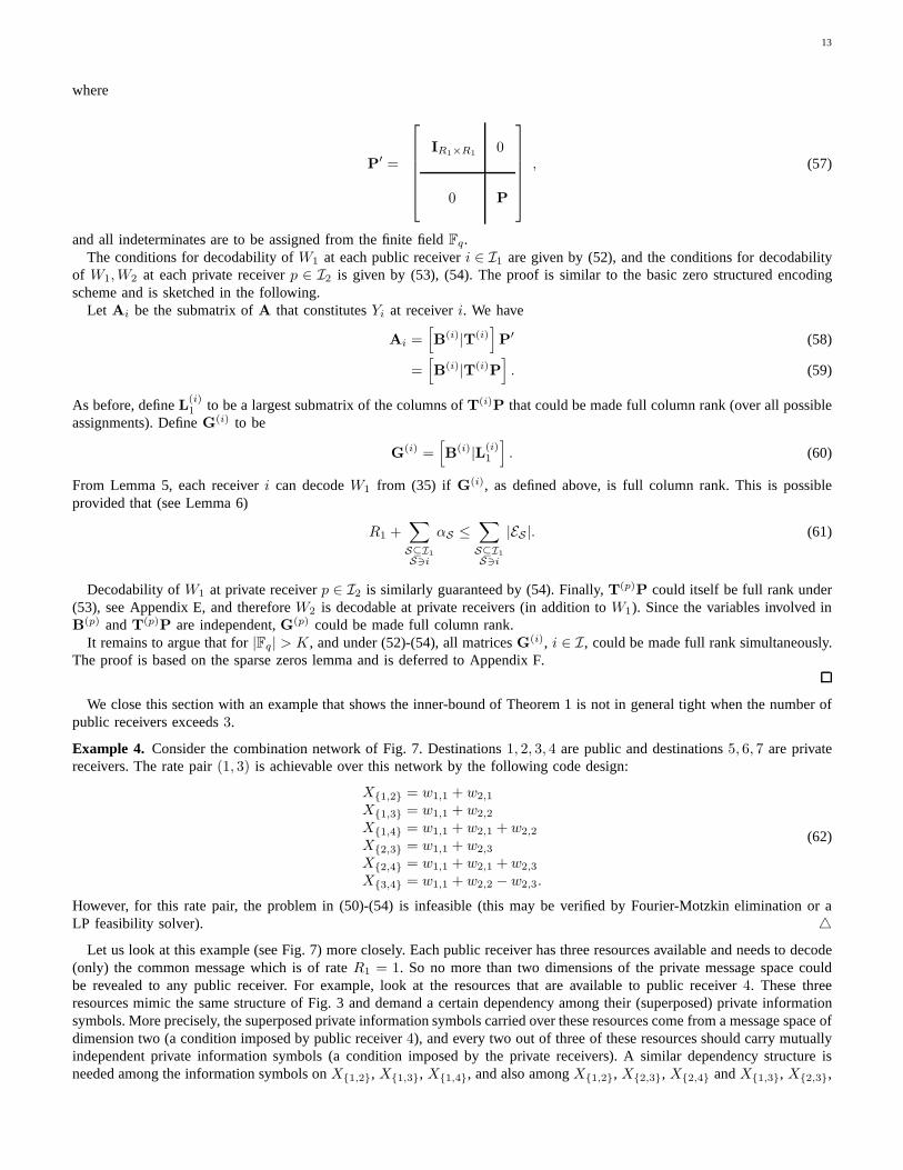
We close this section with an example that shows the inner-bound of Theorem 1 is not in general tight when the number ofpublic receivers exceeds3.

Example 4. Consider the combination network of Fig. 7. Destinations1, 2, 3, 4 are public and destinations5, 6, 7 are privatereceivers. The rate pair(1, 3) is achievable over this network by the following code design:

X{1,2} = w1,1 + w2,1

X{1,3} = w1,1 + w2,2

X{1,4} = w1,1 + w2,1 + w2,2

X{2,3} = w1,1 + w2,3

X{2,4} = w1,1 + w2,1 + w2,3

X{3,4} = w1,1 + w2,2 − w2,3.

(62)

However, for this rate pair, the problem in (50)-(54) is infeasible (this may be verified by Fourier-Motzkin eliminationor aLP feasibility solver). △

Let us look at this example (see Fig. 7) more closely. Each public receiver has three resources available and needs to decode(only) the common message which is of rateR1 = 1. So no more than two dimensions of the private message space couldbe revealed to any public receiver. For example, look at the resources that are available to public receiver4. These threeresources mimic the same structure of Fig. 3 and demand a certain dependency among their (superposed) private informationsymbols. More precisely, the superposed private information symbols carried over these resources come from a message space ofdimension two (a condition imposed by public receiver4), and every two out of three of these resources should carry mutuallyindependent private information symbols (a condition imposed by the private receivers). A similar dependency structure isneeded among the information symbols onX{1,2}, X{1,3}, X{1,4}, and also amongX{1,2}, X{2,3}, X{2,4} andX{1,3}, X{2,3},

14

S

W1 = [w1,1]

W2 = [w2,1, w2,2, w2,3]

D1 D2 D3 D4 D5 D6 D7

X{1,2} X{1,3} X{1,4} X{2,3} X{2,4} X{3,4}

Fig. 7: The innerbound of Theorem 1 is not tight form > 3 public receivers: while the rate pair(1, 3) is not in the rate-regionof Theorem 1, the code in (62) is a construction that allows communication at ratesR1 = 1, R2 = 3.

X{3,4}. This shows a more involved dependency structure among the revealed partial private information symbols, and explainswhy our modified encoding scheme of Theorem 1 cannot be optimal for this example.

Now consider the coding scheme of (62) that achieves(1, 3) (we assume|Fq| > 2). This code ensures decodability ofW1, w2,1, w2,2 at public receiver1, decodability ofW1, w2,1, w2,3 at public receiver2, decodability ofW1, w2,2, w2,3 at publicreceiver3, decodability ofW1, w2,1 + w2,2, w2,1 + w2,3 at public receiver4 and decodability ofW1,W2 at private receivers5, 6, 7. The (partial) private information that is revealed to different subsets of the public receivers is also as follows: no privateinformation is revealed to subsets{1, 2, 3, 4}, {1, 2, 3}, {1, 2, 4}, {1, 3, 4}, {2, 3, 4}, the private information revealed to{1, 2}is w2,1, to {1, 3} is w2,2, to {2, 3} is w2,3, to {1, 4} is w2,1 + w2,2, to {2, 4} is w2,1 + w2,3, to {3, 4} is w2,2 − w2,3, andfinally no private information is revealed to{1}, {2}, {3}, {4}. Now, it becomes clearer that the dependency structure thatisneeded among the partial private information may, in general, be more involved than is allowed by our simple pre-encodingtechnique.

In the next section, we develop a simple block Markov encoding scheme to tackle Example 4, and derive a new achievablescheme for the general problem.

V. A B LOCK MARKOV ENCODING SCHEME

A. Main idea

We saw that the difficulty in the code design stems mainly fromthe following tradeoff: On one hand, private receiversrequire all the public and private information symbols and therefore prefer to receive mutually independent information overtheir resources. On the other hand, each public receiver requires that its received encoded symbols do not depend on “toomany” private information symbols. This imposes certain dependencies among the encoded symbols of the public receivers’resources .

The main idea in this section is to capture these dependencies over sequential blocks, rather than capturing it through thestructure of the one-time (one-block) code. For this, we usea block Markov encoding scheme. We start with an example whereboth previous schemes were sub-optimal and we show the optimality of the block Markov encoding scheme for it.

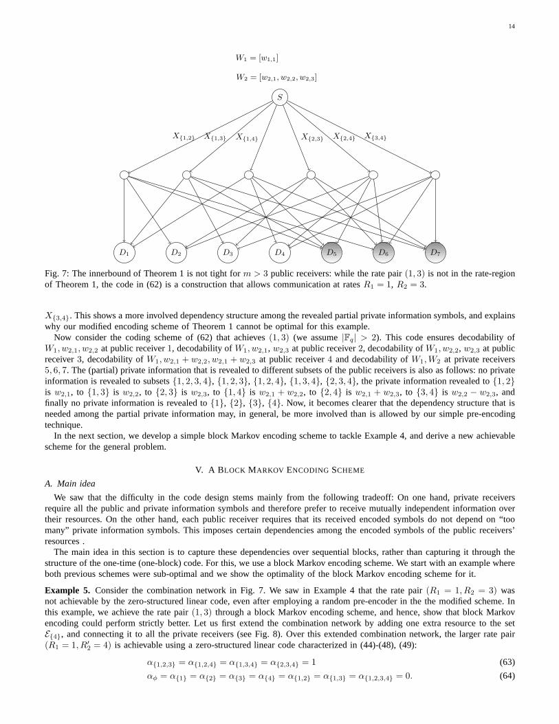
Example 5. Consider the combination network in Fig. 7. We saw in Example4 that the rate pair(R1 = 1, R2 = 3) wasnot achievable by the zero-structured linear code, even after employing a random pre-encoder in the the modified scheme.Inthis example, we achieve the rate pair(1, 3) through a block Markov encoding scheme, and hence, show thatblock Markovencoding could perform strictly better. Let us first extend the combination network by adding one extra resource to the setE{4}, and connecting it to all the private receivers (see Fig. 8).Over this extended combination network, the larger rate pair(R1 = 1, R′

2 = 4) is achievable using a zero-structured linear code characterized in (44)-(48), (49):

α{1,2,3} = α{1,2,4} = α{1,3,4} = α{2,3,4} = 1 (63)

αφ = α{1} = α{2} = α{3} = α{4} = α{1,2} = α{1,3} = α{1,2,3,4} = 0. (64)

15

S

W1[t+ 1] = [w1,1[t+ 1]]

W ′2[t+ 1] = [w′

2,1[t+ 1], w′2,2[t+ 1], w′

2,3[t + 1], w′t+12,4 [t + 1]]

D1 D2 D3 D4 D5 D6 D7

X{1,2}[t] X{1,3}[t] X{1,4}[t] X{2,3}[t] X{2,4}[t] X{3,4}[t] X{4}[t]

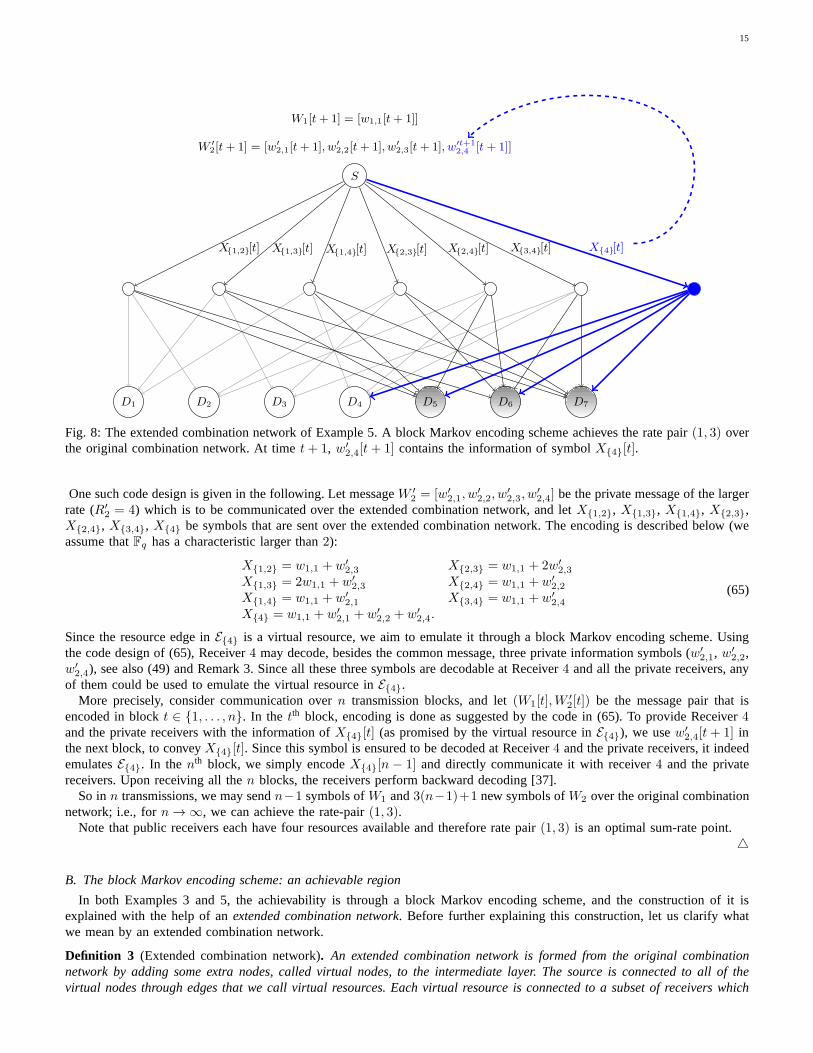
Fig. 8: The extended combination network of Example 5. A block Markov encoding scheme achieves the rate pair(1, 3) overthe original combination network. At timet+ 1, w′

2,4[t+ 1] contains the information of symbolX{4}[t].

One such code design is given in the following. Let messageW ′2 = [w′

2,1, w′2,2, w

′2,3, w

′2,4] be the private message of the larger

rate (R′2 = 4) which is to be communicated over the extended combination network, and letX{1,2}, X{1,3}, X{1,4}, X{2,3},

X{2,4}, X{3,4}, X{4} be symbols that are sent over the extended combination network. The encoding is described below (weassume thatFq has a characteristic larger than2):

X{1,2} = w1,1 + w′2,3 X{2,3} = w1,1 + 2w′

2,3

X{1,3} = 2w1,1 + w′2,3 X{2,4} = w1,1 + w′

2,2

X{1,4} = w1,1 + w′2,1 X{3,4} = w1,1 + w′

2,4

X{4} = w1,1 + w′2,1 + w′

2,2 + w′2,4.

(65)

Since the resource edge inE{4} is a virtual resource, we aim to emulate it through a block Markov encoding scheme. Usingthe code design of (65), Receiver4 may decode, besides the common message, three private information symbols (w′

2,1, w′2,2,

w′2,4), see also (49) and Remark 3. Since all these three symbols are decodable at Receiver4 and all the private receivers, any

of them could be used to emulate the virtual resource inE{4}.More precisely, consider communication overn transmission blocks, and let(W1[t],W

′2[t]) be the message pair that is

encoded in blockt ∈ {1, . . . , n}. In the tth block, encoding is done as suggested by the code in (65). To provide Receiver4and the private receivers with the information ofX{4}[t] (as promised by the virtual resource inE{4}), we usew′

2,4[t+ 1] inthe next block, to conveyX{4}[t]. Since this symbol is ensured to be decoded at Receiver4 and the private receivers, it indeedemulatesE{4}. In thenth block, we simply encodeX{4}[n − 1] and directly communicate it with receiver4 and the privatereceivers. Upon receiving all then blocks, the receivers perform backward decoding [37].

So inn transmissions, we may sendn−1 symbols ofW1 and3(n−1)+1 new symbols ofW2 over the original combinationnetwork; i.e., forn→∞, we can achieve the rate-pair(1, 3).

Note that public receivers each have four resources available and therefore rate pair(1, 3) is an optimal sum-rate point.△

B. The block Markov encoding scheme: an achievable region

In both Examples 3 and 5, the achievability is through a blockMarkov encoding scheme, and the construction of it isexplained with the help of anextended combination network. Before further explaining this construction, let us clarify whatwe mean by an extended combination network.

Definition 3 (Extended combination network). An extended combination network is formed from the originalcombinationnetwork by adding some extra nodes, called virtual nodes, tothe intermediate layer. The source is connected to all of thevirtual nodes through edges that we call virtual resources.Each virtual resource is connected to a subset of receivers which

16

we refer to as the end-destinations of that virtual resource. This subset is chosen, depending on the structure of the originalcombination network and the target rate pair, through an optimization problem that we will address later in this section.

The idea behind extending the combination network is as follows. The encoding is such that in order to decode the commonand private messages in blockt, each receiver may need the information that it will decode in block t+1 (recall that receiversperform backward decoding). So, the source wants to design both its outgoing symbols in blockt and the side informationthat the receiver will have in blockt+1. This is captured by designing a code over an extended combination network, wherethe virtual resources play, in a sense, the role of the side information.

Over the extended combination networks, we will design ageneral multicast code(as opposed to one for nested messagesets). We will only consider multicast codes based on basic linear superposition coding to emulate the virtual resources (seeRemark 4). We further elaborate on this in the following.

Definition 4 (Emulatable virtual resources). Given an extended combination network and a general multicast code over it,a virtual resourcev is called emulatable if the multicast code allows reliable communication at a rate of at least1 to allend-destinations of that virtual resource (over the extended combination network). We call a set of virtual resources emulatableif they are all simultaneously emulatable.

We now outline the steps in devising a block Markov encoding scheme for this problem.

1) Add a set of virtual resources to the original combinationnetwork to form an extended combination network.2) Design a general (as opposed to one for nested message sets) multicast code over the extended combination network

such that all the virtual resources are emulatable.3) Use the multicast code to make all the virtual resources emulatable. More precisely, use the information symbols in

block t + 1 to also convey the information carried on the virtual resources in blockt. Use the remaining informationsymbols to communicate the common and private information symbols.

An achievable rate-region could then be found by optimizingover the virtual resources and the multicast code.Formulating this problem in its full generality is not the goal of this section. We instead aim to construct a simple block

Markov encoding scheme, show its advantages in code design,and characterize a region achievable by it. To this end, weconfine ourselves to the following two assumptions: (i) the virtual resources that we introduce are connected to all privatereceivers and different subsets of public receivers, and (ii) the multicast code that we design over the extended combinationnetwork is a basic linear superposition code along the linesof the codes in Section IV-C.

In order to devise our simple block Markov scheme, we first create an extended combination network by adding for everyS ⊆ I1, βS many virtual resources which are connected to all the private receivers and all the public receivers inS ⊆ I1 (andonly those). We denote this subset of virtual resources byVS .

Over this extended combination network, we then design a (general) multicast code. We say that a multicast code achievesrate tuple(R1, α{1,...,m}, . . . , αφ) over the extended combination network, if it reliably communicates a message of rateR1 toall receivers, and independent messages of ratesαS , S ⊆ I1, to all public receivers inS and all private receivers. To designsuch a multicast code, we use a basic linear superposition code (i.e., a zero-structured encoding matrix). It turns out that therate tuple(R1, α{1,...,m}, . . . , αφ) is achievable if the following inequalities are satisfied (see Remark 3):

Decodability constraints at public receivers:∑

S⊆I1

S∋i

αS ≤∑

S∈Λ

αS+∑

S∈Λc

S∋i

(|ES |+ βS) , ∀Λ ⊆ {{i}⋆} superset saturated, ∀i ∈ I1 (66)

R1 +∑

S⊆I1

S∋i

αS ≤∑

S⊆I1

S∋i

(|ES |+ βS) , ∀i ∈ I1 (67)

Decodability constraints at private receivers:

R′2 ≤

∑

S∈Λ

αS +∑

S∈Λc

(|ES,p|+ βS) , ∀Λ ⊆ 2I1 superset saturated, ∀p ∈ I2 (68)

R1 +R′2 ≤

∑

S⊆I1

(|ES,p|+ βS) , ∀p ∈ I2, (69)

where

R′2 =

∑

S⊆I1

αS . (70)

Given such a multicast code, we find conditions for the virtual resources to be emulatable. The proof is relegated toAppendix G.

17

Lemma 8. Given an extended combination network withβS virtual resourcesVS , S ⊆ I1, and a multicast code designthat achieves the rate tuple(R1, α{1,...,m}, . . . , αφ), all virtual resources are emulatable provided that the following set ofinequalities hold.

∑

S∈Λ

βS ≤∑

S∈Λ

αS , ∀Λ ⊆ 2I1superset saturated. (71)

It remains to characterize the common and private rates thatour simple block Markov encoding scheme achieves over theoriginal combination network. To do so, we disregard the information symbols that are used to emulate the virtual resources,for they bring redundant information, and characterize theremaining rate of the common and private information symbols. Inthe above scheme, this is simply(R1, R

′2−∑

S⊆I1βS), where the real valued parametersαS , βS satisfy inequalities (66)-(70)

and the following non-negativity constraints:

αS ≥ 0, (72)

βS ≥ 0. (73)

To simplify the representation, we defineγS = αS − βS , ∀S ⊆ I1, and then eliminateα’s andβ’s from all inequalitiesinvolved. We thus have the following theorem.

Theorem 2. The rate pair(R1, R2) is achievable if there exist parametersγS , S ⊆ I1, such that they satisfy the followinginequalities:

∑

S∈Λ

γS ≥ 0, ∀Λ ⊆ 2I1 superset saturated (74)

R2 =∑

S⊆I1

γS , (75)

Decodability constraints at public receivers:∑

S⊆I1

S∋i

γS ≤∑

S∈Λ

γS +∑

S∈Λc

S∋i

|ES |, ∀Λ ⊆ {{i}⋆} superset saturated, ∀i ∈ I1 (76)

R1 +∑

S⊆I1

S∋i

γS ≤∑

S⊆I1

S∋i

|ES |, ∀i ∈ I1 (77)

Decodability constraints at private receivers:

R2 ≤∑

S∈Λ

γS +∑

S∈Λc

|ES,p|, ∀Λ ⊆ 2I1 superset saturated, ∀p ∈ I2 (78)

R1 +R2 ≤∑

S⊆I1

|ES,p|, ∀p ∈ I2. (79)

Comparing the rate-regions in Theorem 1 and Theorem 2, we seethat the former has a more relaxed set of inequalitiesin (74) while the latter is more relaxed in inequalities (76). Although the two regions are not comparable in general, it turnsout that form ≤ 3, the two rate-regions coincide and characterize the capacity region (see Theorem 4 and Theorem 5).Furthermore, the combination network in Fig. 7 serves as an instance where the rate-region in Theorem 2 includes rate pairsthat are not included in the region of Theorem 1 (see Examples4 and 5).

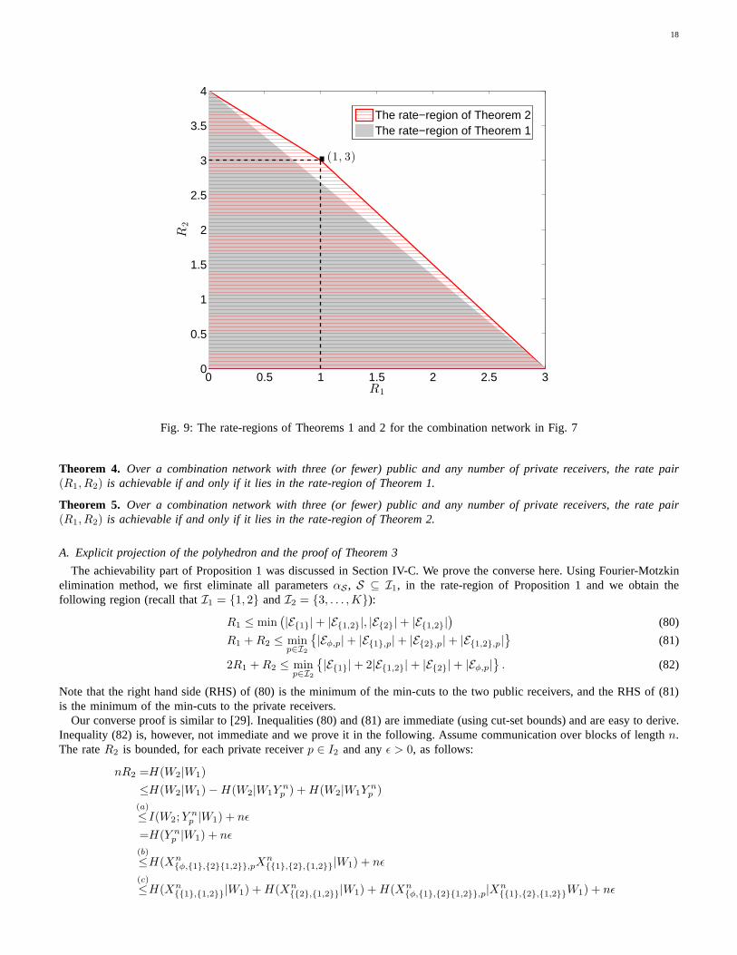
Fig. 9 plots the rate-regions of Theorem 1 and Theorem 2 for the network of Fig. 7. The grey region is the region ofTheorem 1 (i.e., achievable using pre-encoding, rate-splitting, and linear superposition coding) and the red shaded region isthe region of Theorem 2 (i.e., achievable using the proposedblock Markov encoding scheme). In this example, the proposedblock Markov encoding scheme strictly outperforms our previous schemes.

Remark 8. It remains open whether the rate-region of Theorem 2 always includes the rate-region of Theorem 1, or not. Weconjecture that this is true.

VI. OPTIMALITY RESULTS

In this section, we prove our optimality results. More precisely, we prove optimality of the zero-structured encoding schemeof Subsection IV-C whenm = 2, optimality of the structured linear code with pre-encoding discussed in Subsection IV-D whenm = 3 (or fewer), and optimality of the block Markov encoding of Section V whenm = 3 (or fewer). This is summarized inthe following theorems.

Theorem 3. Over a combination network with two public and any number of private receivers, the rate pair(R1, R2) isachievable if and only if it lies in the rate-region of Proposition 1.

18

0 0.5 1 1.5 2 2.5 30

0.5

1

1.5

2

2.5

3

3.5

4

R1

R2

The rate−region of Theorem 2The rate−region of Theorem 1

(1, 3).

Fig. 9: The rate-regions of Theorems 1 and 2 for the combination network in Fig. 7

Theorem 4. Over a combination network with three (or fewer) public and any number of private receivers, the rate pair(R1, R2) is achievable if and only if it lies in the rate-region of Theorem 1.

Theorem 5. Over a combination network with three (or fewer) public and any number of private receivers, the rate pair(R1, R2) is achievable if and only if it lies in the rate-region of Theorem 2.

A. Explicit projection of the polyhedron and the proof of Theorem 3

The achievability part of Proposition 1 was discussed in Section IV-C. We prove the converse here. Using Fourier-Motzkinelimination method, we first eliminate all parametersαS , S ⊆ I1, in the rate-region of Proposition 1 and we obtain thefollowing region (recall thatI1 = {1, 2} andI2 = {3, . . . ,K}):

R1 ≤ min(

|E{1}|+ |E{1,2}|, |E{2}|+ |E{1,2}|)

(80)

R1 +R2 ≤ minp∈I2

{

|Eφ,p|+ |E{1},p|+ |E{2},p|+ |E{1,2},p|}

(81)

2R1 +R2 ≤ minp∈I2

{

|E{1}|+ 2|E{1,2}|+ |E{2}|+ |Eφ,p|}

. (82)

Note that the right hand side (RHS) of (80) is the minimum of the min-cuts to the two public receivers, and the RHS of (81)is the minimum of the min-cuts to the private receivers.

Our converse proof is similar to [29]. Inequalities (80) and(81) are immediate (using cut-set bounds) and are easy to derive.Inequality (82) is, however, not immediate and we prove it inthe following. Assume communication over blocks of lengthn.The rateR2 is bounded, for each private receiverp ∈ I2 and anyǫ > 0, as follows:

nR2 =H(W2|W1)

≤H(W2|W1)−H(W2|W1Ynp ) +H(W2|W1Y

np )

(a)

≤ I(W2;Ynp |W1) + nǫ

=H(Y np |W1) + nǫ

(b)

≤H(Xn{φ,{1},{2}{1,2}},pX

n{{1},{2},{1,2}}|W1) + nǫ

(c)

≤H(Xn{{1},{1,2}}|W1) +H(Xn

{{2},{1,2}}|W1) +H(Xn{φ,{1},{2}{1,2}},p|X

n{{1},{2},{1,2}}W1) + nǫ

19

S

D1

C1

C2

C3

D2 D3

e1 e2 e3 e4

Fig. 10: The rate-region in Theorem 3 evaluates toR1 ≤ 2, R1 +R2 ≤ 4 and2R1 +R2 ≤ 5.

(d)

≤H(Xn{{1},{1,2}}) +H(Xn

{{2},{1,2}})− 2nR1 +H(Xn{φ,{1},{2}{1,2}},p|X

n{{1},{2},{1,2}}W1) + 3nǫ

(e)

≤H(Xn{{1},{1,2}}) +H(Xn

{{2},{1,2}})− 2nR1 +H(Xnφ,p) + 3nǫ

(f)

≤n(|E{1}|+ |E{1,2}|) + n(|E{2}|+ |E{1,2}|)− 2nR1 + n(|Eφ,p|) + 3nǫ,

In the above chain of inequalities, step(a) follows from Fano’s inequality. Step(b) follows because the received sequenceY np is given by all symbols inXn

{φ,{1},{2}{1,2}},p and we further add all symbolsXn{1,2},Xn

{1},Xn{2}. Step(c) follows from

sub-modularity of entropy. Step(d) is a result of (83)-(85), below, where (85) is due to Fano’s inequality (W1 should berecoverable with arbitrarily small error probability fromXn

{{1},{1,2}}).

H(Xn{{1},{1,2}}|W1) =H(Xn

{{1},{1,2}}W1)− nR1 (83)

=H(Xn{{1},{1,2}}) +H(W1|X

n{{1},{1,2}})− nR1 (84)

≤H(Xn{{1},{1,2}}) + nǫ− nR1. (85)

Similarly, we haveH(Xn

{{2},{1,2}}|W1) ≤ H(Xn{{2},{1,2}})− nR1 + nǫ.

Step(e) follows from the fact that for anyS ⊆ I1, XnS,p is contained inXn

S (by definition) and that conditioning reduces theentropy. Finally, step(f) follows because each entropy termH(Xn

S ) is bounded byn|S| (remember that all rates are writtenin units of log2 |Fq| bits).

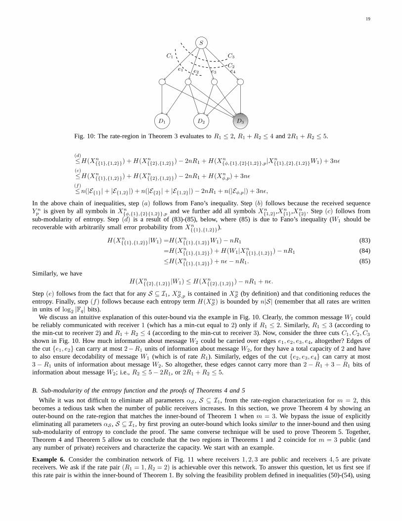
We discuss an intuitive explanation of this outer-bound viathe example in Fig. 10. Clearly, the common messageW1 couldbe reliably communicated with receiver1 (which has a min-cut equal to2) only if R1 ≤ 2. Similarly, R1 ≤ 3 (according tothe min-cut to receiver2) andR1 +R2 ≤ 4 (according to the min-cut to receiver3). Now, consider the three cutsC1, C2, C3

shown in Fig. 10. How much information about messageW2 could be carried over edgese1, e2, e3, e4, altogether? Edges ofthe cut{e1, e2} can carry at most2−R1 units of information about messageW2, for they have a total capacity of2 and haveto also ensure decodability of messageW1 (which is of rateR1). Similarly, edges of the cut{e2, e3, e4} can carry at most3 − R1 units of information about messageW2. So altogether, these edges cannot carry more than2 − R1 + 3 − R1 bits ofinformation about messageW2; i.e., R2 ≤ 5− 2R1, or 2R1 +R2 ≤ 5.

B. Sub-modularity of the entropy function and the proofs of Theorems 4 and 5

While it was not difficult to eliminate all parametersαS , S ⊆ I1, from the rate-region characterization form = 2, thisbecomes a tedious task when the number of public receivers increases. In this section, we prove Theorem 4 by showing anouter-bound on the rate-region that matches the inner-bound of Theorem 1 whenm = 3. We bypass the issue of explicitlyeliminating all parametersαS , S ⊆ I1, by first proving an outer-bound which lookssimilar to the inner-bound and then usingsub-modularity of entropy to conclude the proof. The same converse technique will be used to prove Theorem 5. Together,Theorem 4 and Theorem 5 allow us to conclude that the two regions in Theorems 1 and 2 coincide form = 3 public (andany number of private) receivers and characterize the capacity. We start with an example.

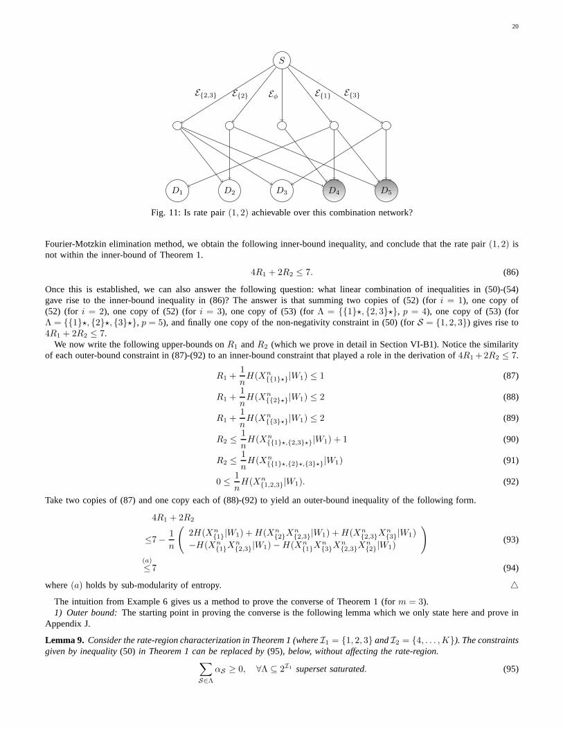
Example 6. Consider the combination network of Fig. 11 where receivers1, 2, 3 are public and receivers4, 5 are privatereceivers. We ask if the rate pair(R1 = 1, R2 = 2) is achievable over this network. To answer this question, let us first see ifthis rate pair is within the inner-bound of Theorem 1. By solving the feasibility problem defined in inequalities (50)-(54), using

20

S

D1 D2 D3 D4 D5

E{1}E{2,3} E{2} E{3}Eφ

Fig. 11: Is rate pair(1, 2) achievable over this combination network?

Fourier-Motzkin elimination method, we obtain the following inner-bound inequality, and conclude that the rate pair(1, 2) isnot within the inner-bound of Theorem 1.

4R1 + 2R2 ≤ 7. (86)

Once this is established, we can also answer the following question: what linear combination of inequalities in (50)-(54)gave rise to the inner-bound inequality in (86)? The answer is that summing two copies of (52) (fori = 1), one copy of(52) (for i = 2), one copy of (52) (fori = 3), one copy of (53) (forΛ = {{1}⋆, {2, 3}⋆}, p = 4), one copy of (53) (forΛ = {{1}⋆, {2}⋆, {3}⋆}, p = 5), and finally one copy of the non-negativity constraint in (50) (for S = {1, 2, 3}) gives rise to4R1 + 2R2 ≤ 7.

We now write the following upper-bounds onR1 andR2 (which we prove in detail in Section VI-B1). Notice the similarityof each outer-bound constraint in (87)-(92) to an inner-bound constraint that played a role in the derivation of4R1+2R2 ≤ 7.

R1 +1

nH(Xn

{{1}⋆}|W1) ≤ 1 (87)

R1 +1

nH(Xn

{{2}⋆}|W1) ≤ 2 (88)

R1 +1

nH(Xn

{{3}⋆}|W1) ≤ 2 (89)

R2 ≤1

nH(Xn

{{1}⋆,{2,3}⋆}|W1) + 1 (90)

R2 ≤1

nH(Xn

{{1}⋆,{2}⋆,{3}⋆}|W1) (91)

0 ≤1

nH(Xn

{1,2,3}|W1). (92)

Take two copies of (87) and one copy each of (88)-(92) to yieldan outer-bound inequality of the following form.

4R1 + 2R2

≤7−1

n

(

2H(Xn{1}|W1) +H(Xn

{2}Xn{2,3}|W1) +H(Xn

{2,3}Xn{3}|W1)

−H(Xn{1}X

n{2,3}|W1)−H(Xn

{1}Xn{3}X

n{2,3}X

n{2}|W1)

)

(93)

(a)

≤ 7 (94)

where(a) holds by sub-modularity of entropy. △

The intuition from Example 6 gives us a method to prove the converse of Theorem 1 (form = 3).1) Outer bound:The starting point in proving the converse is the following lemma which we only state here and prove in

Appendix J.

Lemma 9. Consider the rate-region characterization in Theorem 1 (whereI1 = {1, 2, 3} andI2 = {4, . . . ,K}). The constraintsgiven by inequality(50) in Theorem 1 can be replaced by(95), below, without affecting the rate-region.

∑

S∈Λ

αS ≥ 0, ∀Λ ⊆ 2I1 superset saturated. (95)

21

By Lemma 9, the rate-region of Theorem 1 is equivalently given by constraints (51)-(54), (95). We now find an outer-boundwhich lookssimilar to this inner-bound.

Lemma 10. Any achievable rate pair(R1, R2) satisfies outer-bound constraints(96)-(99) for any givenǫ > 0.

1

nH(Xn

Λ|W1) ≥ 0, ∀Λ ⊆ 2I1 superset saturated (96)

R1 +1

nH(Xn

{{i}⋆}|W1) ≤∑

S∈{{i}⋆}

|ES |+ ǫ, ∀i ∈ I1 (97)

R2 ≤1

nH(Xn

Λ|W1) +∑

S∈Λc

|ES,p|+ ǫ, ∀Λ ⊆ 2I1 superset saturated, ∀p ∈ I2 (98)

R1 +R2 ≤∑

S⊆I1

|ES,p|+ ǫ, ∀p ∈ I2. (99)

Remark 9. Notice the similarity of inequalities(96), (97), (98), (99) with constraints(95), (52), (53), (54), respectively. Weprovide no similar outer-bound for the inner-bound constraint (51) because it is redundant3.

Proof. Inequalities in (96) hold by the positivity of entropy. To show inequalities in (97), we boundR1 for each public receiveri ∈ I1 as follows:

nR1 =H(W1) (100)

=H(W1)−H(W1|Yni ) +H(W1|Y

ni ) (101)

(a)

≤ I(W1;Yni ) + nǫ (102)

=I(W1;Xn{{i}⋆}) + nǫ (103)

=H(Xn{{i}⋆})−H(Xn

{{i}⋆}|W1) + nǫ (104)

(b)

≤n

∑

S∈{{i}⋆}

|ES |

−H(Xn{{i}⋆}|W1) + nǫ. (105)

In the above chain of inequalities,(a) follows from Fano’s inequality and(b) follows by bounding the cardinality of thealphabet set ofXn

{{i}⋆} and usingH(X) ≤ log |X |, whereX is the alphabet set ofX . In a similar manner, we have thefollowing bound onnR1 + nR2 for each private receiverp which proves inequality (99).

nR1 + nR2 =H(W1W2) (106)

≤I(W1W2;Ynp ) + nǫ (107)

=I(W1W2;Xn{φ⋆},p) + nǫ (108)

=H(Xn{φ⋆},p) + nǫ (109)

≤n

∑

S∈{φ⋆}

|ES,p|

+ nǫ. (110)

Finally, we boundR2 to obtain the inequalities in (98). In the following, we havep ∈ I2, Λ ⊆ 2I1 , andǫ > 0.

nR2 =H(W2|W1) (111)

=H(W2|W1)−H(W2|W1Ynp ) +H(W2|W1Y

np ) (112)

(a)

≤ I(W2;Ynp |W1) + nǫ (113)

=I(W2;Xn{φ⋆},p|W1) + nǫ (114)

=H(Xn{φ⋆},p|W1) + nǫ (115)

(b)

≤H(Xn{φ⋆},pX

nΛ|W1) + nǫ (116)

=H(XnΛ|W1) +H(Xn

{φ⋆},p|XnΛW1) + nǫ (117)

(c)

≤H(XnΛ|W1) +H(Xn

Λc,p) + nǫ (118)

3This inequality is redundant because it is the only inequality that contains the free variableαφ.

22

(d)

≤H(XnΛ|W1) + n

(

∑

S∈Λc

|ES,p|

)

+ nǫ. (119)

In the above chain of inequalities, step(a) follows from Fano’s inequality. Step(b) holds for any subsetΛ ⊆ 2I1 and inparticular subsets which are superset saturated. Step(c) follows because conditioning decreases entropy. Step(d) follows byby bounding the cardinality of the alphabet set ofXn

Λc,p and usingH(X) ≤ log |X |, whereX is the alphabet set ofX .

We shall use sub-modularity of the entropy function to provethat the outer bound of Lemma 10 and the inner bound ofTheorem 1 match. Let us introduce a few techniques, as it may not be clear how sub-modularity could be used in full generality.

2) Sub-modularity lemmas:We adopt some definitions and results from [36] and prove a lemma that takes a central rolein the converse proof in Section VI-B3.

Let [F] be a family of multi-sets4 of subsets of{s1, . . . , sN}. Given a multi-setΓ = [Γ1, . . . ,Γl] (whereΓi ⊆ {s1, . . . , sN},i = 1, . . . , l), let Γ′ be a multi-set obtained fromΓ by replacingΓi andΓj by Γi ∩ Γj andΓi ∪Γj for somei, j ∈ {1, . . . , l},i 6= j. The multi-setΓ′ is then said to be anelementary compressionof Γ. The elementary compression is, in particular,non-trivial if neitherΓi ⊆ Γj nor Γj ⊆ Γi. A sequence of elementary compressions gives acompression. A partial order≥ isdefined over[F] as follows.Γ ≥ Λ if Λ is a compression ofΓ (equality if and only if the compression is composed of alltrivial elementary compressions). A simple consequence ofthe sub-modularity of the entropy function is the followinglemma[36, Theorem 5].

Lemma 11. [36, Theorem 5] LetX = (Xsi)N1 be a sequence of random variables withH(X) finite and letΓ and Λ be

finite multi-sets of subsets of{s1, . . . , sN} such thatΓ ≥ Λ. Then∑

Γ∈Γ

H(XΓ) ≥∑

Λ∈Λ

H(XΛ).

For our converse, we consider the family of multi-sets of subsets of2I1 whereI1 = {1, 2, 3}. We denote multi-sets bybold greek capital letters (e.g.,Γ andΛ), subsets of2I1 by greek capital letters (e.g.,Γi, Σ andΛ), and elements of2I1 bycalligraphic capital letters (e.g.,S and T ). Over a family of multi-sets of subsets of2I1 , we definemulti-sets of saturatedpatternandmulti-sets of standard patternas follows.

Definition 5 (Multi-sets of saturated pattern). A multi-set (of subsets of2I1) is said to be of (superset) saturated patternif all its elements are superset saturated. E.g., forI1 = {1, 2, 3}, we have that multi-sets[{{1}, {1, 2}, {1, 3}, {1, 2, 3}}]and [{{1}, {1, 2}, {1, 3}, {1, 2, 3}}, {{2, 3}, {1, 2, 3}}] are both of saturated pattern, but not[{{2}, {1, 2}, {1, 2, 3}}] (since itsonly element is not superset saturated as{2, 3} is missing from it) or[{{1}, {2}, {1, 2}, {1, 3}, {2, 3}, {1, 2, 3}}, {{1}, {1, 2}}](since{{1}, {1, 2}} is not superset saturated).

Definition 6 (Multi-sets of standard pattern). A multi-set (of subsets of2I1) is said to be of standard pattern if its ele-ments are all of the form{S ⊆ I1 : S ∋ i}, for somei ∈ I1. E.g., both multi-sets[{{1}, {1, 2}, {1, 3}, {1, 2, 3}}] and[{{1}, {1, 2}, {1, 3}, {1, 2, 3}}, {{2}, {1, 2}, {2, 3}, {1, 2, 3}}] are of standard pattern, but not multi-sets[{{1, 2}, {1, 2, 3}}]or [{{1}, {2}, {1, 2}, {1, 3}, {2, 3}, {1, 2, 3}}].

Definition 7 (Balanced pairs of multi-sets). We say that multi-setsΓ andΛ are a balanced pair if∑

Γ∈Γ1S∈Γ =

∑

Λ∈Λ1S∈Λ,

for all setsS ∈ 2I1 .

Remark 10. One observes that (i) multi-sets of standard pattern are also of saturated pattern, (ii) the set of all multi-sets ofsaturated pattern is closed under compression, (iii) if a multi-set Λ is a compression of a multi-setΓ, then they are balanced,and (iv) two multi-sets of standard pattern are balanced if and only if they are equal.

Let us look at step(a) in inequality (94) in this formulation. Consider the familyof multi-sets of subsets of2{1,2,3},and in particular, the multi-setΓ = [{{1}}, {{1}}, {{2}, {2, 3}}, {{3}, {2, 3}}]. After the following non-trivial elementarycompressions, the multi-setΛ = [{{1}, {2, 3}}, {{1}, {2}, {3}, {2, 3}}] is obtained:

Γ =[{{1}}, {{1}}, {{2}, {2, 3}}, {{3}, {2, 3}}] (120)

≥[{{1}}, {{1}, {2}, {2, 3}}, {{3}, {2, 3}}] =: Γ′ (121)

≥[{{1}}, {{1}, {2}, {3}, {2, 3}}, {{2, 3}}] =: Γ′′ (122)

≥[{{1}, {2, 3}}, {{1}, {2}, {3}, {2, 3}}] =: Λ. (123)

Therefore, we haveΓ ≥ Λ and by Lemma 11,∑

Γ∈ΓH(Xn

Γ |W1) ≥∑

Λ∈ΛH(Xn

Λ|W1). Thus, step(a) of inequality (94)follows.

Here, we develop an alternative visual tool. Associate a graph GΓ to every multi-setΓ. The graph is formed as follows.Each node of the graph represents one set inΓ, and is labeled by it. Two nodes are connected by an edge if andonly if

4Multi-set is a generalization of the notion of a set in which members are allowed to appear more than once.

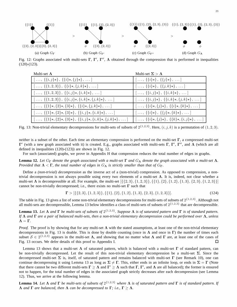
23

{{1}} {{1}}

{{2}, {2, 3}}{{3}, {2, 3}}

(a) GraphGΓ

{{1}} {{1}, {2}, {2, 3}}

φ {{3}, {2, 3}}

>

(b) GraphGΓ′

{{1}}{{1}, {2}, {2, 3}, {3}}

φ {{2, 3}}

>

(c) GraphGΓ′′

{{1}, {2, 3}}{{1}, {2}, {2, 3}, {3}}

φ φ

>

(d) GraphGΛ

Fig. 12: Graphs associated with multi-setsΓ, Γ′, Γ′′, Λ obtained through the compression that is performed in inequalities(120)-(123).

Multi-set Λ Multi-set Σ > Λ

[ . . . , {{i, j}⋆} , {{i}⋆, {j}⋆} , . . . ] [ . . . , {{i}⋆} , {{j}⋆} , . . . ]

[ . . . , {{1, 2, 3}} , {{i}⋆, {j, k}⋆} , . . . ] [ . . . , {{i}⋆} , {{j, k}⋆} , . . . ]

[ . . . , {{1, 2, 3}} , {{i, j}⋆, {i, k}⋆} , . . . ] [ . . . , {{i, j}⋆} , {{i, k}⋆} , . . . ]

[ . . . , {{1, 2, 3}} , {{i, j}⋆, {i, k}⋆, {j, k}⋆} , . . . ] [ . . . , {{i, j}⋆} , {{i, k}⋆, {j, k}⋆} , . . . ]

[ . . . , {{1}⋆, {2}⋆, {3}⋆} , {{i}⋆, {j, k}⋆} , . . . ] [ . . . , {{i}⋆, {j}⋆} , {{i}⋆, {k}⋆} , . . . ]

[ . . . , {{1}⋆, {2}⋆, {3}⋆} , {{i, j}⋆, {i, k}⋆} , . . . ] [ . . . , {{i}⋆} , {{j}⋆, {k}⋆} , . . . ]

[ . . . , {{1}⋆, {2}⋆, {3}⋆} , {{i, j}⋆, {i, k}⋆, {j, k}⋆} , . . . ] [ . . . , {{i}⋆, {j}⋆} , {{k}⋆, {i, j}⋆} , . . . ]

Fig. 13: Non-trivial elementary decompressions for multi-sets of subsets of2{1,2,3}. Here,(i, j, k) is a permutation of(1, 2, 3).

neither is a subset of the other. Each time an elementary compression is performed on the multi-setΓ, a compressed multi-setΓ′ (with a new graph associated with it) is created. E.g., graphs associated with multi-setsΓ, Γ′, Γ′′, andΛ (which are all

defined in inequalities (120)-(123)) are shown in Fig. 12.For such (associated) graphs, we prove in Appendix H that compression reduces the total number of edges in graphs.

Lemma 12. Let GΓ denote the graph associated with a multi-setΓ andGΛ denote the graph associated with a multi-setΛ.Provided thatΛ < Γ, the total number of edges inGΛ is strictly smaller than that ofGΓ.

Define a(non-trivial) decompressionas the inverse act of a (non-trivial) compression. As opposed to compression, a non-trivial decompression is not always possible using every two elements of a multi-setΛ. It is, indeed, not clear whether amulti-setΛ is decompressible at all. For example, the multi-set[{{2, 3}, {1, 2, 3}}, {{1}, {2}, {1, 2}, {1, 3}, {2, 3}, {1, 2, 3}}]cannot be non-trivially decompressed; i.e., there exists no multi-setΓ such that

Γ > [{{2, 3}, {1, 2, 3}}, {{1}, {2}, {1, 2}, {1, 3}, {2, 3}, {1, 2, 3}}]. (124)

The table in Fig. 13 gives a list of some non-trivial elementary decompressions for multi-sets of subsets of2{1,2,3}. Although notall multi-sets are decompressible, Lemma 13 below identifies a class of multi-sets of subsets of2{1,2,3} that are decompressible.

Lemma 13. Let Λ andΓ be multi-sets of subsets of2{1,2,3}. SupposeΛ is of saturated pattern andΓ is of standard pattern.If Λ andΓ are a pair of balanced multi-sets, then a non-trivial elementary decompression could be performed overΛ, unlessΛ = Γ.

Proof. The proof is by showing that for any multi-setΛ with the stated assumptions, at least one of the non-trivialelementarydecompressions in Fig. 13 is doable. This is done by double counting (once inΛ and once inΓ) the number of times eachsubsetS ∈ 2{1,2,3} appears in the multi-setΛ, and showing that no matter whatΛ andΓ are, at least one of the cases ofFig. 13 occurs. We defer details of this proof to Appendix I.

Lemma 13 shows that a multi-setΛ of saturated pattern, which is balanced with a multi-setΓ of standard pattern, canbe non-trivially decompressed. Let the result of this non-trivial elementary decompression be a multi-setΣ. Since thedecompressed multi-setΣ is, itself, of saturated pattern and remains balanced with multi-set Γ (see Remark 10), one cancontinue decompressing it using Lemma 13 as long asΣ 6= Γ. This, either ends in an infinite loop, or ends inΣ = Γ (Notethat there cannot be two different multi-setsΓ ≥ Λ andΓ′ ≥ Λ such thatΓ, Γ′, andΛ are all balanced); the former is ensurednot to happen, for the total number of edges in the associatedgraph strictly decreases after each decompression (see Lemma12). Thus, we arrive at the following lemma.

Lemma 14. Let Λ andΓ be multi-sets of subsets of2{1,2,3} whereΛ is of saturated pattern andΓ is of standard pattern. IfΛ andΓ are balanced, thenΛ can be decompressed toΓ; i.e., Γ ≥ Λ.

24

We are now ready to prove Theorem 4.3) proof of Theorem 4:The rate-region of Theorem 1 can be obtained explicitly by applying Fourier-Motzkin elimination to

(52)-(54) and (95) to eliminate parametersαS . This gives a set of inequalities of the formm1R1 +m2R2 ≤ E, each obtainedby summing potentially multiple copies of constraints (52)-(54), (95), so that all variablesαS , S ⊆ I1, get eliminated. Toshow a converse for each such inner-bound inequality,m1R1 + m2R2 ≤ E, take copies of the corresponding outer-boundconstraints (96)-(99) and sum them up to yield an outer-bound inequality of the form

m1R1 +m2R2 +1

n

∑

Γ∈Γ

H(XnΓ |W1)

≤ E +1

n

∑

Λ∈Λ

H(XnΛ|W1) (125)

whereΓ is a multi-set of standard pattern andΛ is a multi-set of saturated pattern, both consisting of subsets of2I1 whereI1 = {1, 2, 3}. Notice thatΓ andΛ are balanced since Fourier-Motzkin elimination ensures that all theαS ’s are eliminated.So by Lemma 14, we have

Λ ≤ Γ (126)

and therefore,∑

Λ∈Λ

H(XnΛ|W1) ≤

∑

Γ∈Γ

H(XnΓ |W1). (127)

Using (127) in the outer-bound inequality (125), we conclude the converse tom1R1 +m2R2 ≤ E, for every such inequalitythat appears in the inner-bound. This concludes the proof.

Remark 11. Lemmas 9, 13, and 14 are valid only form ≤ 3, and Lemmas 11, 10, and 12 hold in general.

Remark 12. The following example serves as a counter example for Lemma 13 whenm > 3. Consider the following multi-setsof subsets of2{1,2,3,4}:

Λ = [{{1} ⋆ {2} ⋆ {3} ⋆ {4}⋆}, {{1, 2} ⋆ {1, 3} ⋆ {2, 4}}, {{1, 4} ⋆ {2, 3} ⋆ {3, 4}⋆}, {{1, 2, 3, 4}}] ,

Γ = [{{1}⋆}, {{2}⋆}, {{3}⋆}, {{4}⋆}].

It is easy to see thatΛ is of saturated pattern,Γ is of standard pattern, and they are balanced. Nevertheless, no elementarydecompression can be performed onΛ.

One could prove Theorem 5 using the same technique. More precisely, Lemma 9 is already implied and Lemma 10 couldaccommodate an outer-bound constraintsimilar to the inner-bound constraint of (76) as follows:

1

nH(Xn

{{i}⋆}|W1) ≤1

nH(Xn

Λ|W1) +1

nH(Xn

Λ|Xn{{i}⋆},W1) (128)

≤1

nH(Xn

Λ|W1) +1

nH(Xn

({{i}⋆}\Λ)) (129)

≤1

nH(Xn

Λ|W1) +∑

S∈Λc

S∋i

|ES |. (130)

The rest of the converse proof follows, as before, by sub-modularity of entropy.

VII. A BLOCK MARKOV ENCODING SCHEME FOR BROADCASTING TWO NESTED MESSAGE SETS OVER BROADCAST

CHANNELS

We extend our coding technique to general broadcast channels. Consider a broadcast channelp(y1, . . . , yK |x) with inputsignalX , outputsY1, . . . , YK whereYi, i ∈ I1, is available to public receiveri andYp, p ∈ I2, is available to private receiverp.

In many cases where the optimal rates of communication are known for broadcasting nested messages, the classical techniquesof rate splitting and superposition coding have proved optimal, and this motivates us, also, to start with such encodingschemes.In particular, in the context of two message broadcast, we split the private message into different piecesWS

2 of ratesαS , S ⊆ I1,whereWS

2 is revealed to all public receivers inS (as well as the private receivers).Xn is then formed by superposition coding.For I1 = {1, 2}, for instance,W {1}

2 andW{2}2 are each independently superposed on(W1,W

{1,2}2 ), andWφ

2 is superposedon all of them to form the input sequenceXn. The rate-region achievable by superposition coding is given by a feasibilityproblem (a straightforward generalization of [39, Theorem8.1]). The rate pair(R1, R2) is achievable if there exist parameters

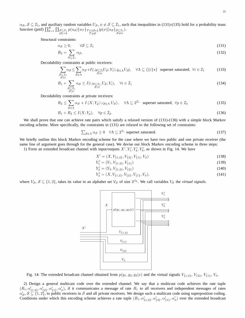
25

αS , S ⊆ I1, and auxiliary random variablesUS , φ 6= S ⊆ I1, such that inequalities in (131)-(135) hold for a probability massfunction (pmf)

∏K

k=1

∏

S⊆I1

|S|=k

p(uS |{uT }T ∈{S⋆}T 6=S

)p(x|{uS}S⊆I1

S6=φ

).

Structural constraints:

αS ≥ 0, ∀S ⊆ I1 (131)

R2 =∑

S⊆I1

αS , (132)

Decodability constraints at public receivers:∑

S⊆I1

S∋i

αS≤∑

S∈Λ

αS+I(∪S⊆I1

S∋i

US ;Yi|∪S∈ΛUS), ∀Λ ⊆ {{i}⋆} superset saturated, ∀i ∈ I1 (133)

R1 +∑

S⊆I1

S∋i

αS ≤ I(∪S⊆I1,S∋i

US ;Yi), ∀i ∈ I1 (134)

Decodability constraints at private receivers:

R2 ≤∑

S∈Λ

αS + I (X ;Yp| ∪S∈Λ US) , ∀Λ ⊆ 2I1 superset saturated, ∀p ∈ I2 (135)

R1 +R2 ≤ I(X ;Yp), ∀p ∈ I2. (136)

We shall prove that one can achieve rate pairs which satisfy arelaxed version of (131)-(136) with a simple block Markovencoding scheme. More specifically, the constraints in (131) are relaxed to the following set of constraints:

∑

S∈Λ αS ≥ 0 ∀Λ ⊆ 2I1 superset saturated. (137)

We briefly outline this block Markov encoding scheme for the case where we have two public and one private receiver (thesame line of argument goes through for the general case). We devise our block Markov encoding scheme in three steps:

1) Form an extended broadcast channel with input/outputsX ′, Y ′1 , Y

′2 , Y

′3 , as shown in Fig. 14. We have

X ′ = (X,V{1,2}, V{2}, V{1}, Vφ) (138)

Y ′1 = (Y1, V{1,2}, V{1}) (139)

Y ′2 = (Y2, V{1,2}, V{2}) (140)

Y ′3 = (X,V{1,2}, V{2}, V{1}, Vφ), (141)

whereVS , S ⊆ {1, 2}, takes its value in an alphabet setVS of size2βS . We call variablesVS the virtual signals.

p(y1, y2, y3|x)

X′

X

V{1,2}

V{1}

V{2}

Vφ

Y ′3

Y ′2

Y ′1

Fig. 14: The extended broadcast channel obtained fromp(y1, y2, y3|x) and the virtual signalsV{1,2}, V{2}, V{1}, Vφ.

2) Design a general multicast code over the extended channel. We say that a multicast code achieves the rate tuple(R1, α

′{1,2}, α

′{2}, α

′{1}, α

′φ), if it communicates a message of rateR1 to all receivers and independent messages of rates

α′S , S ⊆ {1, 2}, to public receivers inS and all private receivers. We design such a multicast code using superposition coding.

Conditions under which this encoding scheme achieves a ratetuple (R1, α′{1,2}, α

′{2}, α

′{1}, α

′φ) over the extended broadcast

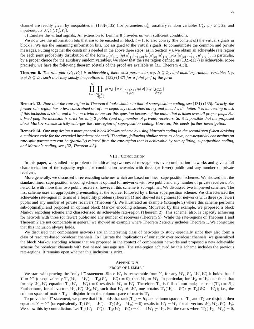
26

channel are readily given by inequalities in (133)-(135) (for parametersα′S , auxiliary random variablesU ′

S , φ 6=S ⊆I1, andinput/outputsX ′, Y ′

1, Y′2,Y

′3 ).

3) Emulate the virtual signals. An extension to Lemma 8 provides us with sufficient conditions.We now use the information bits that are to be encoded in blockt+1, to also convey (the content of) the virtual signals in

block t. We use the remaining information bits, not assigned to the virtual signals, to communicate the common and privatemessages. Putting together the constraints needed in the above three steps (as in Section V), we obtain an achievable rate regionfor each joint probability distribution of the formp(u′

{1,2})p(u′{1}|u

′{1,2})p(u

′{2}|u

′{1,2})p(x

′|u′{2}, u

′{1}, u

′{1,2}). In particular,

by a proper choice for the auxiliary random variables, we show that the rate region defined in (132)-(137) is achievable. Moreprecisely, we have the following theorem (details of the proof are available in [32, Theorem 4.3]).

Theorem 6. The rate pair(R1, R2) is achievable if there exist parametersαS , S ⊆ I1, and auxiliary random variablesUS ,φ 6= S ⊆ I1, such that they satisfy inequalities in(132)-(137) for a joint pmf of the form

K∏

k=1

∏

S⊆I1

|S|=k

p(uS |{uT }T ∈{S⋆}T 6=S

)p(x|{uS}S⊆I1

S6=φ

).

Remark 13. Note that the rate-region in Theorem 6 looks similar to that of superposition coding, see(131)-(135). Clearly, theformer rate-region has a less constrained set of non-negativity constraints onαS and includes the latter. It is interesting to askif this inclusion is strict, and it is non-trivial to answer this question because of the union that is taken over all proper pmfs. Fora fixed pmf, the inclusion is strict form ≥ 3 public (and any number of private) receivers. So it is possible that the proposedblock Markov scheme strictly enlarges the rate-region of superposition coding. However, this needs further investigation.

Remark 14. One may design a more general block Markov scheme by using Marton’s coding in the second step (when devisinga multicast code for the extended broadcast channel). Therefore, following similar steps as above, non-negativity constraints onrate-split parameters can be (partially) relaxed from the rate-region that is achievable by rate-splitting, superposition coding,and Marton’s coding, see [32, Theorem 4.3].

VIII. C ONCLUSION

In this paper, we studied the problem of multicasting two nested message sets over combination networks and gave a fullcharacterization of the capacity region for combination networks with three (or fewer) public and any number of privatereceivers.

More generally, we discussed three encoding schemes which are based on linear superposition schemes. We showed that thestandard linear superposition encoding scheme is optimal for networks with two public and any number of private receivers. Fornetworks with more than two public receivers, however, thisscheme is sub-optimal. We discussed two improved schemes. Thefirst scheme uses an appropriate pre-encoding at the source,followed by a linear superposition scheme. We characterized theachievable rate-region in terms of a feasibility problem (Theorem 1) and showed its tightness for networks with three (or fewer)public and any number of private receivers (Theorem 4). We illustrated an example (Example 5) where this scheme performssub-optimally, and proposed an optimal block Markov encoding scheme. Motivated by this example, we proposed a blockMarkov encoding scheme and characterized its achievable rate-region (Theorem 2). This scheme, also, is capacity achievingfor network with three (or fewer) public and any number of receivers (Theorem 5). While the rate-regions of Theorem 1 andTheorem 2 are not comparable in general, we showed an examplewhere Theorem 2 strictly includes Theorem 1. We conjecturethat this inclusion always holds.

We discussed that combination networks are an interesting class of networks to study especially since they also form aclass of resource-based broadcast channels. To illustratethe implications of our study over broadcast channels, we generalizedthe block Markov encoding scheme that we proposed in the context of combination networks and proposed a new achievablescheme for broadcast channels with two nested message sets.The rate-region achieved by this scheme includes the previousrate-regions. It remains open whether this inclusion is strict.

APPENDIX APROOF OFLEMMA 1

We start with proving the “only if” statement. SinceW1 is recoverable fromY , for anyW1,W2,W′1,W

′2 it holds that if

Y = Y ′ (or equivalentlyT1(W1 −W ′1) + T2(W2 −W ′

2) = 0), thenW1 = W ′1. In particular, forW2 = W ′

2 one finds thatfor any W1,W

′1 equationT1(W1 −W ′

1) = 0 results inW1 = W ′1. Therefore,T1 is full column rank; i.e., rank(T1) = R1.

Furthermore, for all vectorsW1,W′1,W2,W

′2 such thatW1 6= W ′

1, one obtainsT1(W1 −W ′1) 6= T2(W

′2 −W2); i.e., the

column space of matrixT2 is disjoint from the column space of matrixT1.To prove the “if” statement, we prove that if it holds that rank(T1) = R1 and column spaces ofT1 andT2 are disjoint, then

equationY = Y ′ (or equivalentlyT1(W1 −W ′1) +T2(W2 −W ′

2) = 0) results inW1 = W ′1 for all vectorsW1,W2,W

′1,W

′2.

We show this by contradiction. LetT1(W1−W ′1)+T2(W2−W ′

2) = 0 andW1 6= W ′1. For the cases whereT2(W2−W ′

2) = 0,

27

we getT1(W1−W ′1) = 0 for W1 6= W ′

1, which contradicts the original assumption of rank(T1) = R1. If T2(W2−W ′2) 6= 0,

thenT1(W1−W ′1)+T2(W2−W ′

2) = 0 implies that there exists at least one non-zero vector in theintersection of the columnspaces ofT1 andT2 which contradicts the assumption that column space ofT1 andT2 are disjoint.

APPENDIX BPROOF OFLEMMA 3

We start with proving that(i) implies (ii). Assume that matrixT is assigned full column rank. Over the equivalent unicastnetwork, we propose a network code that constitutes a transfer matrix (from nodeA to nodeB) exactly equal to the full-rankmatrix T: First, let each outgoing edge of the source carry one uncoded symbol of the message. Then, let the firstr{1,2} rowsof matrix T specify the local encoding matrix at noden′

{1,2}. Similarly, let the secondr{2}, the thirdr{1}, and the lastrφ setof rows of matrixT specify the local encoding matrices at nodesn′

{2}, n′{1}, andn′

φ, respectively. Note that the zero structureof matrix T, which is given in equation (22), ensures that this is a well defined construction. It follows thatT is the transfermatrix from nodeA to nodeB and, since it is full column rank, the encoded message can be decoded at sink nodeB.

Statement(ii) also implies(i) and the proof is by construction. If a message of ratec could be sent over the equivalentunicast network (from nodeA to nodeB), then there arec edge disjoint paths from the sourceA to the sinkB. Each suchpath matches one of the outgoing edges of source nodeA to one of the incoming edges of sink nodeB. We call this matchingbetween the outgoing edges of the source and the incoming edges of the sink matchingM and we note that its size isc.We use this matching to fill the indeterminates of matrixT with 0 − 1. First of all, note that each columnj of matrix T

corresponds to an outgoing edge of the source, sayej, and each rowi of matrix T corresponds to an incoming edge of thesink, saye′i. So each entry(i, j) of matrix T is priorly set to zero if and only if edgesej and e′j cannot be matched. Now,put a1 in entry (i, j) of matrix T if edgeej is matched to edgee′j over the matchingM . Since matchingM has a size equalto c, matrix T is made full column rank.

APPENDIX CPROOF OFLEMMA 4

Consider all (edge-) cuts separating the source nodeA from the sink nodeB. Since the intermediate edges all have infinitecapacity, the minimum cut does not contain any edges from them. One can verify the following fact over Fig. 6: If an edge(n′

S′ , B), S ′ ⊆ {1, . . . , t}, does not belong to the cut, then all edges(A, nS) whereS ⊇ S ′ belong to that cut. So each(finite-valued) cut corresponds to a subset of the nodesn′

S in the third layer. Denoting this subset of nodes by{n′S}S∈Γ, for

someΓ ⊆ 2{1,...,t}, we have the value of the cut given by∑

S∈Γ

rS +∑

S⊇S′, S′∈Γc

cS . (142)

It is not difficult to verify that the (inclusion-wise) minimal cuts are derived for setsΓc that are superset saturated. RenamingΓc asΛ concludes the proof.

APPENDIX DPROOF OFLEMMA 6

Let ri denote the number of rows inG(i); i.e., let ri =∑

S⊆I1 S∋i |ES |. In the matrixG(i) = [B(i)|L(i)1 ], first select an

assignment for the columns ofL(i)1 that makes them linearly independent (such an assignment exists from construction). Since

the element variables inL(i)1 are independent of those inB(i), G(i) can be made full-rank just by pickingR1 vectors from

Fri , linearly independent from the columns ofL(i)

1 , for the columns ofB(i). This is possible since rank(B(i)) is at most∑

S⊆I1 S∋i αS which is bounded byri −R1 (by assumption).

APPENDIX EDECODABILITY CONSTRAINTS FOR PRIVATE RECEIVERS INTHEOREM 1

For simplicity of notation, we give the proof for the case where m = 2. We prove thatT(p)P could be made full column

rank if and only if messageW2 could be unicast over the network of Fig. 15. In this network the outgoing edges of the sourceand the incoming edges of the sink are all of unit capacity andthe bold edges in the middle are of infinite capacity. DefineT

(p)′ := T(p)

P which is given by

T(p)′ =

α{1,2}←→

α{1}↔

α{2}↔

αφ

↔

0 0 00 0

0 0

llll

|E{1,2},p|

|E{1},p|

|E{2},p|

|Eφ,p|

· P.(143)

28

A

source

n{1,2} n{2} n{1}nφ

n′{1,2},p

n′{2},p n′

{1},p n′φ,p

B

sink

α{1,2} α{2} α{1} (αφ)+

|E{1,2},p||E{2},p| |E{1},p| |Eφ,p|

Fig. 15: Source nodeA communicates a message of rateR2 to the sink node,B.

Think of matrixP as the local transfer matrix at source nodeA. Also, think of the matrix formed by the first|E{1,2},p| rowsof T(p)′ as the local transfer matrix at intermediate noden{1,2},p, the matrix formed by the second|E{1},p| rows ofT(p)′ asthe local transfer matrix at intermediate noden{1} and so on. Notice the equivalence between matrixT

(p)′ and the transfermatrix imposed by a linear network code from nodeA to nodeB over the network of Fig. 15, and conclude that messageW2

is decodable if and only if messageW2 could be unicast fromA to B. Decodability conditions at receiverp can, therefore, beinferred from the min-cut separating nodesA andB over the network of Fig. 15. Lemma 4 gives this min-cut by the followingexpression.

min

minΛ⊂2I1

Λsuperset saturated

∑

S∈Λ

αS +∑

S∈Γc

|ES,p|,∑

S∈2I1 , S6=φ

αS + (αφ)+

. (144)

One can verify thatR2 is smaller than the expression in (144), provided that inequalities in (53) hold.

APPENDIX FAPPLICATION OF THESPARSEZEROSLEMMA TO THE PROOF OFTHEOREM 1

We constructed matricesG(i), i ∈ I and reduced the problem to making all these matrices simultaneously full-rank. MatricesG

(i) have their entries defined by the variables inA andP. We also discussed that each of these matrices could be madefull column rank. This implies that there exists a square submatrix of eachG(i), sayG(i)

s , that could be made full-rank. LetP(i) be the polynomial corresponding to the determinant ofG

(i)s , andP =

∏

i P(i). Given that there exists an assignment for

the variables such that each individual polynomialP(i) is non-zero, we can conclude from the sparse zeros lemma thatthereexists an assignment such that all polynomials are simultaneously non-zero. We can furthermore provide an upper bound onthe required size forF. This is done next by finding the degree of each polynomialP(i) in each variable.

For i ∈ I1, since all variables inG(i)s are independent of each other, the desired degree is at most1. For P(p), p ∈ I2,

also, we can show that the maximum degree in each variable is1. To see this, we proceed as follows. Recall that forp ∈ I2,G

(p) = T(p)

P. Let us denote the(i, j)th entry ofG(p) by gi,j . So eachgi,j =∑

l ti,lpl,j , whereti,l refers to the(i, l)th entryof T(p) andpl,j refers to the(l, j)th entry ofP. Using Laplace expansion, we have

detG(p)s =

∑

i

(−1)i+jgi,j detG(p)i,j , (145)

wheredetGi,j is the matrix obtained fromG(p)s after removing theith row and thej th column. Now, note thatdetGi,j is

not a function of variables{ti,l}l (which are indeed variables ofA), nor is it a function of variables{pl,j}l. Thus, the degreeof P(p) is at most1 in each of the variables ofA andP.

Let us construct the polynomialP =∏

i∈I P(i). EachP(i) is of degree at most1 in each variable. So, the degree ofP is

at mostK in each variable. From the sparse zeros lemma [38, Lemma 2.3], F need only be such that|F| ≥ K.

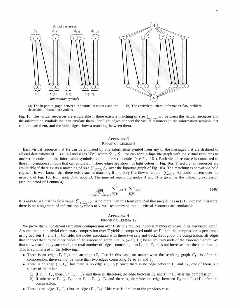
29

βφ

︷ ︸︸ ︷

Virtual resources

Information symbols

β{1}︷︸︸︷

β{2}︷ ︸︸ ︷

β{1,2}︷︸︸︷

αφ

︸︷︷︸

α{1}

︸ ︷︷ ︸

α{2}

︸︷︷︸

α{1,2}

︸ ︷︷ ︸

(a) The bi-partite graph between the virtual resources and thedecodable information symbols.

A

B

(b) The equivalent unicast information flow problem.

Fig. 16: The virtual resources are emulatable if there exists a matching of size∑

S⊆I1βS between the virtual resources and

the information symbols that can emulate them. The light edges connect the virtual resources to the information symbolsthatcan emulate them, and the bold edges show a matching between them.

APPENDIX GPROOF OFLEMMA 8

Each virtual resourcev ∈ VS can be emulated by one information symbol from any of the messages that are destined toall end-destinations ofv; i.e., all messagesW ′S′

2 whereS ′ ⊇ S. One can form a bipartite graph with the virtual resources asone set of nodes and the information symbols as the other set of nodes (see Fig. 16a). Each virtual resource is connected tothose information symbols that can emulate it. These edges are shown in light colour in Fig. 16a. Therefore, all resources areemulatable if there exists a matching of size

∑

S⊆I1βS over the bipartite graph of Fig. 16a. The matching is shown via bold

edges. It is well-known that there exists such a matching if and only if a flow of amount∑

S⊆I1βS could be sent over the

network of Fig. 16b from nodeA to nodeB. The min-cut separating nodesA andB is given by the following expression(see the proof of Lemma 4):

min∀S⊆I1

Γ superset saturated

∑

S∈Γ

αS +∑

S∈Γc

βS . (146)

It is easy to see that the flow value,∑

S⊆I1βS , is no more than this term provided that inequalities in (71)hold and, therefore,

there is an assignment of information symbols to virtual resources so that all virtual resources are emulatable.

APPENDIX HPROOF OFLEMMA 12

We prove that a non-trivial elementary compression overΓ strictly reduces the total number of edges in its associatedgraph.Assume that a non-trivial elementary compression overΓ yields a compressed multi-setΓ′, and the compression is performedusing two setsΓi andΓj . Consider the nodes associated with these two sets and track, throughout the compression, all edgesthat connect them to the other nodes of the associated graph.Let Γk ( 6= Γj ,Γj) be an arbitrary node of the associated graph. Wefirst show that for any such node, the total number of edges connecting it toΓi andΓj does not increase after the compression.This is summarized in the following.

• There is an edge(Γi,Γk) and an edge(Γj ,Γk): In this case, no matter what the resulting graphGΓ′ is after thecompression, there cannot be more than two edges connectingΓk to Γi andΓj.

• There is an edge(Γi,Γk) but there is no edge(Γj ,Γk): Since there is no edge betweenΓj andΓk, one of them is asubset of the other.

1) If Γj ⊆ Γk, thenΓi ∩ Γj ⊆ Γk and there is, therefore, no edge betweenΓk andΓi ∩ Γj after the compression.2) If otherwiseΓj ⊇ Γk, then Γi ∪ Γj ⊇ Γk and there is, therefore, no edge betweenΓk and Γi ∪ Γj after the

compression.

• There is no edge(Γi,Γk) but an edge(Γj ,Γk): This case is similar to the previous case.

30

• There is neither an edge(Γi,Γk) nor an edge(Γj ,Γk): In this case, we have either of the following possibilities.

1) If Γi ⊆ Γk andΓj ⊆ Γk, then bothΓi ∪ Γj andΓi ∩ Γj are subsets ofΓk and there is no edge connectingΓk toΓi ∩ Γj or Γi ∪ Γj overGΓ′ .

2) If Γi ⊆ Γk andΓj ⊇ Γk, thenΓi ∪ Γj ⊇ Γk andΓi ∩ Γj ⊆ Γk and there is, therefore, no edge connectingΓk toΓi ∩ Γj or Γi ∪ Γj overGΓ′ .

3) If Γi ⊇ Γk andΓj ⊆ Γk, then similar to the previous case one concludes that there is no edge connectingΓk toΓi ∩ Γj or Γi ∪ Γj overGΓ′ .

4) If Γi ⊇ Γk and Γj ⊇ Γk, then bothΓi ∪ Γj and Γi ∩ Γj are supersets ofΓk and there is, therefore, no edgeconnectingΓk to their replacementsΓi ∩ Γj or Γi ∪ Γj overGΓ′ .

Besides, edges betweenΓk andΓk′ , wherek, k′ /∈ {i, j}, remain unaffected. Since the compression is non-trivial,nodesΓi

andΓj have been connected overGΓ and are no longer connected overGΓ′ . So, the total number of edges inGΓ is strictlysmaller thanGΓ, and this concludes the proof.

APPENDIX IPROOF OFLEMMA 13

Let Λ be a multiset of2{1,2,3} with saturated pattern,Γ be a multi-set of2{1,2,3} with standard pattern, andΓ andΛ bebalanced and such thatΛ 6= Γ. We prove that no matter whatΓ andΛ are, at least one of the cases of the table in Fig. 13must hold forΛ, and therefore a non-trivial elementary decompression ofΛ is feasible.

Let us first count, in two different ways (once inΛ and once inΓ), the number of times a setS ⊆ I1 appears in the setsof multi-setsΛ andΓ. First of all, definenS , S ⊆ I1, to be the number of all setsΓ ∈ Γ that containS as an element. Oneobserves (from the standard pattern of multi-setΓ) that nS =

∑

i∈S n{i}. Similarly, definemΛ, Λ ∈ Λ, to be the number oftimes the setΛ appears in the multi-setΛ. For simplicity of notation, we usemΛ∪ to denote the number of all setsΛ′ inΛ which are of the formΛ′ = Λ ∪ Σ whereΣ ⊆ 2I1 is superset saturated, andΛ 6⊇ Σ. For example,m{{1,2}⋆}∪ counts thenumber of all sets such as{{1, 2}⋆}, {{1, 3}⋆, {1, 2}⋆}, {{2, 3}⋆, {1, 2}⋆}, {{2, 3}⋆, {1, 3}⋆, {1, 2}⋆}, and{{3} ⋆ {1, 2}⋆}in Λ, but not{{1}⋆} or {{1}⋆, {3}⋆}.

Since multi-setsΓ andΛ are balanced, the number of sets inΓ which contain a setS is equal to the number of the sets inΛ which contain it. Thus, counting the number of sets inΓ andΛ which contain{i} and{i, j} as elements, we obtain thefollowing relationship. In the following, we assume(i, j, k) to be a permutation of(1, 2, 3).

n{i} = m{{i}⋆}∪ (147)

n{i,j} = m{{i}⋆}∪ +m{{j}⋆}∪ −m{{i}⋆,{j}⋆}∪ +m{{i,j}⋆}∪ (148)

Sincen{i,j} = n{i} + n{j}, we conclude from (147) and (148) the following equation.

m{{i}⋆,{j}⋆}∪ = m{{i,j}⋆}∪ (149)

Similarly, counting the number of sets inΓ andΛ which contain{1, 2, 3} as an element, we arrive at the following equation.

n{1,2,3} = m{{1}⋆}∪ +m{{2}⋆}∪ +m{{3}⋆}∪ +m{{1,2}⋆}∪ +m{{1,3}⋆}∪ +m{{2,3}⋆}∪ +

+m{{1,2,3}⋆}∪ −m{{1}⋆,{2}⋆}∪ −m{{1}⋆,{3}⋆}∪ −m{{2}⋆,{3}⋆}∪ −m{{1}⋆,{2,3}⋆}∪ +

−m{{2}⋆,{1,3}⋆}∪ −m{{3}⋆,{1,2}⋆}∪ −m{{1,2}⋆,{1,3}⋆}∪ −m{{1,2}⋆,{2,3}⋆}∪ +

−m{{1,3}⋆,{2,3}⋆}∪ +m{{1,2}⋆,{1,3}⋆,{2,3}⋆}∪ +m{{1}⋆,{2}⋆,{3}⋆}∪ (150)

Usingn{1,2,3} = n{1} + n{2} + n{3}, equation (147) and inserting (149) into (150), we obtain

m{{1,2,3}⋆}∪ +m{{1}⋆,{2}⋆,{3}⋆}∪ = m{{1}⋆,{2,3}⋆}∪ +m{{2}⋆,{1,3}⋆}∪ +m{{3}⋆,{1,2}⋆}∪ +

+m{{1,2}⋆,{1,3}⋆}∪ +m{{1,2}⋆,{2,3}⋆}∪ +m{{1,3}⋆,{2,3}⋆}∪

−m{{1,2}⋆,{1,3}⋆,{2,3}⋆}∪. (151)

Now we write eachmΛ∪ in terms ofmΛ’s to derive the equation of our interest.

m{{1,2,3}⋆} +m{{1}⋆,{2}⋆,{3}⋆} = m{{1}⋆,{2,3}⋆} +m{{2}⋆,{1,3}⋆} +m{{3}⋆,{1,2}⋆} +m{{1,2}⋆,{1,3}⋆} +

+m{{1,2}⋆,{1,3}⋆,{2,3}⋆} +m{{1,2}⋆,{2,3}⋆} +m{{1,2}⋆,{1,3}⋆,{2,3}⋆} +

+m{{1,3}⋆,{2,3}⋆} +m{{1,2}⋆,{1,3}⋆,{2,3}⋆} −m{{1,2}⋆,{1,3}⋆,{2,3}⋆}

= m{{1}⋆,{2,3}⋆} +m{{2}⋆,{1,3}⋆} +m{{3}⋆,{1,2}⋆} +m{{1,2}⋆,{1,3}⋆} +

+m{{1,2}⋆,{2,3}⋆} +m{{1,3}⋆,{2,3}⋆} + 2m{{1,2}⋆,{1,3}⋆,{2,3}⋆} (152)

Observe from equality (152) that if there is a non-zero term,mΛ1, on the left hand, there is at least one other non-zero term,

mΛ2, on the right hand of the equality. No matter whatΛ1 andΛ2 are, see that we are in one of the decompression cases

31

in the table in Fig. 13. If both sides of equality (152) are zero, then one concludes thatm{{i}⋆,{j}⋆}∪ = m{{i}⋆,{j}⋆} andm{{i,j}⋆}∪ = m{{i,j}⋆} and therefore, by equation (149), we have another equation of interest.

m{{i}⋆,{j}⋆} = m{{i,j}⋆} (153)

Again, if m{{i}⋆,{j}⋆} is non-zero so ism{{i,j}⋆}, and we have the first case described in the table of Fig. 13.We have proved that a non-trivial elementary decompositionis possible unless all terms in (152) and (153) are zero, and all

terms in (152) and (153) are zero only ifΛ = Γ which contradicts the hypothesis.

APPENDIX JPROOF OFLEMMA 9

Let us call the rate-region characterized in Theorem 1 (whenI1 = {1, 2, 3}) regionR1 and the rate-region obtained fromrelaxing inequality (50) to inequality (95) (whenI1 = {1, 2, 3}) regionR2. Clearly,R1 ⊆ R2. It is, therefore, sufficient toshow thatR2 ⊆ R1. Both rate-regionsR1 andR2 are in terms of feasibility problems. In this sense, rate pair (R1, R2) belongsto R1 if and only if feasibility problem1 (characterized by inequalities (50)-(54)) is feasible. Similarly, rate pair(R1, R2)belongs toR2 if and only if feasibility problem2 (characterized by inequalities (95), (51)-(54)) is feasible.

In order to show thatR2 ⊆ R1, we show that if(R1, R2) is such that there exists a solution,αS , S ⊆ I1, to feasibilityproblem2, then there also exists a solutionα′

S , S ⊆ I1, to feasibility problem1. Note that problem1 varies from problem2only in the non-negativity constraints on parametersα′

S , φ 6= S ⊆ I1. The goal is to construct parametersα′S (from parameters

αS) such that besides satisfying constraints (51)-(54), theyall become non-negative except forαφ.We prove the existence of a solutionα′

S , S ⊆ 2I1 , by construction. This construction is done recursively. We start from asolution to feasibility problem2, αS , S ⊆ I1, and, at each step, we propose a solutionα′

S , S ⊆ I1, that is still a solution tofeasibility problem2 but is “strictly less negative” (excludingαφ). So after enough number of steps, we end up with a set ofparametersα′

S , S ⊆ I1, that satisfies (51)-(54) and also satisfies the non-negativity constraints in (50).

1. First, we setα′S = αS for all S ⊆ {1, 2, 3}. All α′

S , S ⊆ {1, 2, 3}, satisfy (51)-(54), (95).α{1,2,3} is ensured to benon-negative by (95) (forΛ = {{1, 2, 3}}).

2. We then choose non-negative parametersα′{i,j}, i, j ∈ {1, 2, 3}. Without loss of generality, take the following three cases,

and setα′S ’s as suggested (other cases are dealt with similarly).

(a) If α{1,2} < 0 andα{1,3} < 0 andα{2,3} < 0:set α′

{1,2,3} = α{1,2,3} + α{1,2} + α{1,3} + α{2,3}, α′{1,2} = α′

{1,3} = α′{2,3} = 0, α′

{i} = α{i}, for i = 1, 2, 3,and α′

φ = αφ. One can verify that allα′S , S ⊆ {1, 2, 3}, satisfy (51)-(54), (95). We outline this verification

in the following. (51), (52), (54), and (95) clearly hold. Weshow how to verify (53) through an example, say,Λ = {{1, 2}, {1, 2, 3}} and somep ∈ I2. From feasibility of problem2, we know thatαS is such that it satisfies(53) for all superset saturated subsetsΛ, and in particular forΛ = {{1, 2}⋆, {1, 3}⋆, {2, 3}⋆}. So, we have

R2 ≤ α{1,2,3} + α{1,2} + α{1,3} + α{2,3} +∑

S∈{φ,{1},{2},{3}}

|ES,p| (154)

= α′{1,2,3} +

∑

S∈{φ,{1},{2},{3}}

|ES,p| (155)

≤ α′{1,2,3} + α′

{1,2} +∑

S∈{{1,3},{2,3},φ,{1},{2},{3}}

|ES,p|. (156)

(b) If α{1,2} < 0 andα{1,3} < 0:setα′

{1,2,3} = α{1,2,3} + α{1,2} + α{1,3}, α′{1,2} = α′

{1,3} = 0, α′{2,3} = α{2,3}, α′

{i} = α{i} for i = 1, 2, 3, andα′φ = αφ. Verify that all α′

S , S ⊆ {1, 2, 3}, satisfy (51)-(54), (95).(c) If α{1,2} < 0:

setα′{1,2,3} = α{1,2,3} + α{1,2}, α′

{1,2} = 0, α′{1,3} = α{1,3}, α′

{2,3} = α{2,3}, α′{i} = α{i} for i = 1, 2, 3, and

α′φ = αφ. Verify that all α′

S , S ⊆ {1, 2, 3}, satisfy (51)-(54), (95).

3. Finally, we choose non-negative parametersα′{i}, i ∈ {1, 2, 3}. This is done recursively, following the procedure below,

for eachα′i < 0, until all α′

{i}, i = 1, 2, 3, are non-negative.δ is assumed a small enough positive number.

(a) If α′{i,j}, α

′{i,k} > 0:

set α′{i} = α′

{i} + δ, α′{i,j} = α′

{i,j} − δ, α′{i,k} = α′

{i,k} − δ, α′{1,2,3} = α′

{1,2,3} + δ, and keep the rest ofα′S ’s unchanged. Verify that allα′

S , S ⊆ {1, 2, 3}, satisfy (51)-(54), (95). We show (53) for one example:Λ ={{1, 2}⋆, {1, 3}⋆} and somep ∈ I2. Since theαS ’s we start with satisfy (53) for any superset saturatedΛ, and inparticular forΛ = {{1}⋆}, we have

R2 ≤ α{1} + α{1,2} + α{1,3} + α{1,2,3} +∑

S∈{φ,{2},{3},{2,3}}

|ES,p| (157)

32

≤ α′{1} + α′

{1,2} + α′{1,3} + α′

{1,2,3} +∑

S∈{φ,{2},{3},{2,3}}

|ES,p| (158)

≤ α′{1,2} + α′

{1,3} + α′{1,2,3} +

∑

S∈{φ,{2},{3},{2,3}}

|ES,p|, (159)

where the last inequality is becauseα′{1} is either still negative, or has just become zero after adding the smallδ.

(b) If α′{i,j} = 0, α′

{i,k} > 0:setα′

{i} = α′{i} + δ, α′

{i,k} = α′{i,k} − δ, and keep the rest ofα′

S ’s unchanged. Verify that allα′S , S ⊆ {1, 2, 3},

satisfy (51)-(54), (95).(c) If α′

{i,j} > 0, α′{i,k} = 0:

setα′{i} = α′

{i} + δ, α′{i,j} = α′

{i,j} − δ, and keep the rest ofα′S ’s unchanged. Verify that allα′

S , S ⊆ {1, 2, 3},satisfy (51)-(54), (95).

(d) If α′{i,j} = 0, α′

{i,k} = 0:setα′

{i} = α′{i} + δ, α′

{1,2,3} = α′{1,2,3} − δ, and keep the rest ofα′

S ’s unchanged. Verify that allα′S , S ⊆ {1, 2, 3},

satisfy (51)-(54), (95).

Note that in step1, we obtain a solution to feasibility problem2 with α{1,2,3} ≥ 0. After step2, the solution is such thatα{1,2}, α{1,3}, α{2,3}, α{1,2,3} are all non-negative. In step3, after each iteration,α{1,2}, α{1,3}, α{2,3}, α{1,2,3} all remainnon-negative and at the same time one negativeα{i} is increased. So after step3, all parametersαS , φ 6= S ⊆ {1, 2, 3},become non-negative. This is the solution to feasibility problem1 that we were looking for.

REFERENCES

[1] T. Cover, “Comments on broadcast channels,”IEEE Trans.Inf. Theory, vol. 44, no. 6, pp. 2524–2530, Oct. 1998.[2] R. Ahlswede, N. Cai, S.-Y. Li, and R. Yeung, “Network information flow,” IEEE Trans.Inf. Theory, vol. 46, no. 4, pp. 1204 –1216, July 2000.[3] H. Weingarten, Y. Steinberg, and S. Shamai, “The capacity region of the gaussian multiple-input multiple-output broadcast channel,”IEEE Trans.Inf.

Theory, vol. 52, no. 9, pp. 3936 –3964, Sept. 2006.[4] A. Avestimehr, S. Diggavi, and D. Tse, “Wireless networkinformation flow: A deterministic approach,”IEEE Trans.Inf. Theory, vol. 57, no. 4, pp.

1872 –1905, Apr. 2011.[5] Y. Geng and C. Nair, “The capacity region of the two-receiver gaussian vector broadcast channel with private and common messages,”IEEE Trans.Inf.

Theory, vol. 60, no. 4, pp. 2087–2104, Apr. 2014.[6] K. Marton, “A coding theorem for the discrete memorylessbroadcast channel,”IEEE Trans.Inf. Theory, vol. 25, no. 3, pp. 306 – 311, May 1979.[7] A. Gohari, A. El Gamal, and V. Anantharam, “On an outer bound and an inner bound for the general broadcast channel,” inIEEE Int. Symp.Inf. Theory,

June 2010, pp. 540 –544.[8] C. Nair and A. El Gamal, “An outer bound to the capacity region of the broadcast channel,”IEEE Trans.Inf. Theory, vol. 53, no. 1, pp. 350 –355, Jan.

2007.[9] Y. Liang, G. Kramer, and H. Poor, “On the equivalence of two achievable regions for the broadcast channel,”IEEE Trans.Inf. Theory, vol. 57, no. 1,

pp. 95 –100, Jan. 2011.[10] T. Chan and A. Grant, “Entropy vectors and network codes,” in IEEE Int. Symp.Inf. Theory, June 2007, pp. 1586–1590.[11] R. W. Yeung,Information TheoryandNetwork Coding, 1st ed. Springer Publishing Company, 2008.[12] L. Song, R. Yeung, and N. Cai, “Zero-error network coding for acyclic networks,”IEEE Trans.Inf. Theory, vol. 49, no. 12, pp. 3129–3139, Dec. 2003.[13] T. Cover, “Broadcast channels,”IEEE Trans.Inf. Theory, vol. 18, no. 1, pp. 2 – 14, Jan. 1972.[14] P. Bergmans, “Random coding theorem for broadcast channels with degraded components,”IEEE Trans.Inf. Theory, vol. 19, no. 2, pp. 197 – 207, Mar.

1973.[15] K. Marton, “The capacity region of deterministic broadcast channels,” inIEEE Int. Symp.Inf. Theory, 1977.[16] M. S. Pinsker, “The capacity region of noiseless broadcast channels,”Probl. Inf. Transm, vol. 14, pp. 97 – 102, 1974.[17] J. Korner and K. Marton, “General broadcast channels with degraded message sets,”IEEE Trans.Inf. Theory, vol. 23, no. 1, pp. 60 – 64, Jan. 1977.[18] S.-Y. Li, R. Yeung, and N. Cai, “Linear network coding,”IEEE Trans.Inf. Theory, vol. 49, no. 2, pp. 371 –381, Feb. 2003.[19] R. Koetter and M. Medard, “An algebraic approach to network coding,” IEEE/ACM Trans.Networking, vol. 11, no. 5, pp. 782 – 795, Oct. 2003.[20] T. Han and K. Kobayashi, “A new achievable rate region for the interference channel,”IEEE Trans.Inf. Theory, vol. 27, no. 1, pp. 49–60, Jan. 1981.[21] H. F. Chong, M. Motani, H. K. Garg, and H. El Gamal, “On theHan-Kobayashi region for the interference channel,”IEEE Trans.Inf. Theory, vol. 57,

no. 7, pp. 3188–3195, July 2008.[22] C. Nair and A. El Gamal, “The capacity region of a class of3-receiver broadcast channels with degraded message sets,” IEEE Trans. Inf. Theory,

vol. 55, no. 10, pp. 4479–4493, Oct. 2009.[23] S. Saeedi Bidokhti and V. Prabhakaran, “Is non-unique decoding necessary?”IEEE Trans.Inf. Theory, vol. 60, no. 5, pp. 2594–2610, May 2014.[24] A. Ramamoorthy and R. D. Wesel, “The single source two terminal network with network coding,”ArXiv e-prints, 2009, available on

http://arxiv.org/abs/0908.2847.[25] C. Ngai and R. Yeung, “Multisource network coding with two sinks,” in Int. Conf. Commun.,Circuits andSys, vol. 1, June 2004, pp. 34 – 37 Vol.1.[26] E. Erez and M. Feder, “Capacity region and network codesfor two receivers multicast with private and common data,” in Workshopon Coding,

CryptographyandCombinatorics, 2003.[27] S. Diggavi and D. Tse, “On opportunistic codes and broadcast codes with degraded message sets,” inIEEE Inf. TheoryWorkshop, Mar. 2006.[28] S. Borade, L. Zheng, and M. Trott, “Multilevel broadcast networks,” in IEEE Int. Symp.Inf. Theory, June 2007, pp. 1151 –1155.[29] V. Prabhakaran, S. Diggavi, and D. Tse, “Broadcasting with degraded message sets: A deterministic approach,” inAnnual Allerton Conf. on Commun.,

Control and Computing, 2007.[30] S. Saeedi Bidokhti, S. Diggavi, C. Fragouli, and V. Prabhakaran, “On degraded two message set broadcasting,” inIEEE Inf. Theory Workshop, Oct.

2009, pp. 406 –410.[31] S. Gheorghiu, S. Saeedi Bidokhti, C. Fragouli, and A. Toledo, “Degraded multicasting with network coding over the combination network,” inIEEE

Int. Symp.Network Coding, 2011, available on http://infoscience.epfl.ch/record/174452.[32] S. Saeedi Bidokhti,Broadcastingand Multicasting NestedMessageSets. PhD dissertation, Ecole Polytechnique Federal de Lausanne, 2012.[33] X. Xu and Y. L. Guan, “Joint routing and random network coding for multi-session networks,” inIEEE Int. Conf. Networks, Dec. 2013, pp. 1–5.[34] T. H. Chan and A. J. Grant, “Network coding capacity regions via entropy functions,”ArXiv e-prints, 2012, available on http://arxiv.org/abs/1201.1062.

33

[35] C. K. Ngai and R. Yeung, “Network coding gain of combination networks,” inIEEE Inf. TheoryWorkshop, Oct. 2004, pp. 283 – 287.[36] P. Balister and B. Bollobas, “Projections, entropy and sumsets,” Combinatorica, vol. 32, no. 2, pp. 125–141, 2012. [Online].Available:

http://dx.doi.org/10.1007/s00493-012-2453-1[37] F. Willems and E. van der Meulen, “The discrete memoryless multiple-access channel with cribbing encoders,”IEEE Trans.Inf. Theory, vol. 31, no. 3,

pp. 313 – 327, May 1985.[38] C. Fragouli and E. Soljanin, “Network coding fundamentals,” Foundationsand Trends in Networking , vol. 2, no. 1, pp. 1–133, 2007. [Online].

Available: http://dx.doi.org/10.1561/1300000003[39] A. El Gamal and Y. H. Kim,Network Information Theory. Cambridge University Press, 2011.