arX

iv:1

404.

1675

v1 [

cs.IT

] 7

Apr

201

41

Distributed MAC Protocol for Cognitive Radio

Networks: Design, Analysis, and Optimization

Le Thanh Tan and Long Bao Le

Abstract

In this paper, we investigate the joint optimal sensing and distributed MAC protocol design problem for cognitive radio

networks. We consider both scenarios with single and multiple channels. For each scenario, we design a synchronized MAC

protocol for dynamic spectrum sharing among multiple secondary users, which incorporates spectrum sensing for protecting

active primary users. We perform saturation throughput analysis for the corresponding proposed MAC protocols that explicitly

capture spectrum sensing performance. Then, we find their optimal configuration by formulating throughput maximization problems

subject to detection probability constraints for primary users. In particular, the optimal solution of the optimization problem returns

the required sensing time for primary users’ protection andoptimal contention window for maximizing total throughputof the

secondary network. Finally, numerical results are presented to illustrate developed theoretical findings in the paperand significant

performance gains of the optimal sensing and protocol configuration.

Index Terms

MAC protocol, spectrum sensing, optimal sensing, throughput maximization, cognitive radio.

I. I NTRODUCTION

Emerging broadband wireless applications have been demanding unprecedented increase in radio spectrum resources. As

a result, we have been facing a serious spectrum shortage problem. However, several recent measurements reveal very low

spectrum utilization in most useful frequency bands [1]. Toresolve this spectrum shortage problem, the Federal Communications

Commission (FCC) has opened licensed bands for unlicensed users’ access. This important change in spectrum regulationhas

resulted in growing research interests on dynamic spectrumsharing and cognitive radio in both industry and academia. In

particular, IEEE has established an IEEE 802.22 workgroup to build the standard for WRAN based on CR techniques [2].

Hierarchical spectrum sharing between primary networks and secondary networks is one of the most widely studied dynamic

spectrum sharing paradigms. For this spectrum sharing paradigm, primary users typically have strictly higher priority than

secondary users in accessing the underlying spectrum. One potential approach for dynamic spectrum sharing is to allow both

The authors are with INRS-EMT, University of Quebec, Montr´eal, Quebec, Canada. Emails:lethanh,long.le@emt.inrs.ca.L. B. Le is the corresponding

author.

2

primary and secondary networks to transmit simultaneouslyon the same frequency with appropriate interference control to

protect the primary network [3], [4]. In particular, it is typically required that a certain interference temperature limit due to

secondary users’ transmissions must be maintained at each primary receiver. Therefore, power allocation for secondary users

should be carefully performed to meet stringent interference requirements in this spectrum sharing model.

Instead of imposing interference constraints for primary users, spectrum sensing can be adopted by secondary users to search

for and exploit spectrum holes (i.e., available frequency bands) [5], [6]. There are several challenging technical issues related

to this spectrum discovery and exploitation problem. On onehand, secondary users should spend sufficient time for spectrum

sensing so that they do not interfere with active primary users. On the other hand, secondary users should efficiently exploit

spectrum holes to transmit their data by using an appropriate spectrum sharing mechanism. Even though these aspects are

tightly coupled with each other, they have not been treated thoroughly in the existing literature.

In this paper, we make a further bold step in designing, analyzing, and optimizing MAC protocols for cognitive radio

networks considering sensing performance captured in detection and false alarm probabilities. Specifically, the contributions of

this paper can be summarized as follows:i) we design distributed synchronized MAC protocols for cognitive radio networks

incorporating spectrum sensing operation for both single and multiple channel scenarios;ii) we analyze saturation throughput

of the proposed MAC protocols;iii) we perform throughput maximization of the proposed MAC protocols against their key

parameters, namely sensing time and minimum contention window; iv) we present numerical results to illustrate performance

of the proposed MAC protocols and the throughput gains due tooptimal protocol configuration.

The remaining of this paper is organized as follows. SectionIII describes system and sensing models. MAC protocol design,

throughput analysis, and optimization for the single channel case are performed in Section IV. The multiple channel case is

considered in Section V. Section VI presents numerical results followed by concluding remarks in Section VII.

II. RELATED WORKS

Various research problems and solution approaches have been considered for a dynamic spectrum sharing problem in the

literature. In [3], [4], a dynamic power allocation problemfor cognitive radio networks was investigated consideringfairness

among secondary users and interference constraints for primary users. When only mean channel gains averaged over shortterm

fading can be estimated, the authors proposed more relaxed protection constraints in terms of interference violation probabilities

for the underlying fair power allocation problem. In [7], information theory limits of cognitive radio channels were derived.

Game theoretic approach for dynamic spectrum sharing was considered in [8], [9].

There is a rich literature on spectrum sensing for cognitiveradio networks (e.g., see [10] and references therein). Classical

sensing schemes based on, for example, energy detection techniques or advanced cooperative sensing strategies [11] where

multiple secondary users collaborate with one another to improve the sensing performance have been investigated in the

literature. There are a large number of papers considering MAC protocol design and analysis for cognitive radio networks

3

[12]-[19] (see [12] for a survey of recent works in this topic). However, these existing works either assumed perfect spectrum

sensing or did not explicitly model the sensing imperfection in their design and analysis. In [5], optimization of sensing and

throughput tradeoff under a detection probability constraint was investigated. It was shown that the detection constraint is met

with equality at optimality. However, this optimization tradeoff was only investigated for a simple scenario with one pair of

secondary users. Extension of this sensing and throughput tradoff to wireless fading channels was considered in [20].

There are also some recent works that propose to exploit cooperative relays to improve sensing and throughput

performance of cognitive radio networks. In particular, a novel selective fusion spectrum sensing and best relay data

transmission scheme was proposed in [21]. Closed-form expression for the spectrum hole utilization efficiency of the

proposed scheme was derived and significant performance improvement compared to other sensing and transmission

schemes was demonstrated through extensive numerical studies. In [22], a selective relay based cooperative spectrum

sensing scheme was proposed that does not require a separatechannel for reporting sensing results. In addition, the

proposed scheme can achieve excellent sensing performancewith controllable interference to primary users. These

existing works, however, only consider a simple setting with one pair of secondary users.

III. SYSTEM AND SPECTRUM SENSING MODELS

In this section, we describe the system and spectrum sensingmodels. Specifically, sensing performance in terms of detection

and false alarm probabilities are explicitly described.

A. System Model

We consider a network setting whereN pairs of secondary users opportunistically exploit available frequency bands, which

belong a primary network, for their data transmission.Note that the optimization model in [5] is a special case of our

model with only one pair of secondary users.In particular, we will consider both scenarios in which one or multiple radio

channels are exploited by these secondary users. We will design synchronized MAC protocols for both scenarios assumingthat

each channel can be in idle or busy state for a predetermined periodic interval, which is referred to as a cycle in this paper.

We further assume that each pair of secondary users can overhear transmissions from other pairs of secondary users (i.e.,

collocated networks). In addition, it is assumed that transmission from each individual pair of secondary users affects one

different primary receiver. It is straightforward to relaxthis assumption to the scenario where each pair of secondaryusers

affects more than one primary receiver and/or each primary receiver is affected by more than one pair of secondary users.The

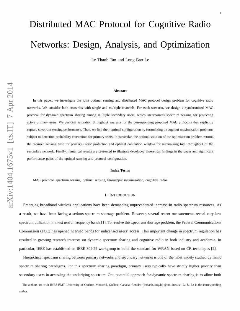
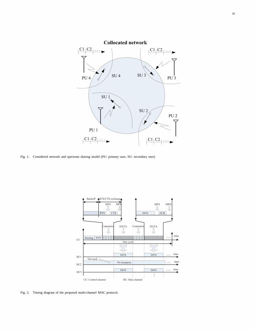
network setting under investigation is shown in Fig. 1. In the following, we will refer to pairi of secondary users as secondary

link i or flow i interchangeably.

Remark 1: In practice, secondary users can change their idle/busy status any time (i.e., status changes can occur

in the middle of any cycle). Our assumption on synchronous channel status changes is only needed to estimate the

4

system throughput. In general, imposing this assumption would not sacrifice the accuracy of our network throughput

calculation if primary users maintain their idle/busy status for sufficiently long time on average. This is actually the

case for many practical scenarios such as in TV bands as reported by several recent studies (see [2] and references

therein). In addition, our MAC protocols developed under this assumption would result in very few collisions with

primary users because the cycle time is quite small comparedto typical active/idle periods of primary users.

B. Spectrum Sensing

We assume that secondary links rely on a distributed synchronized MAC protocol to share available frequency channels.

Specifically, time is divided into fixed-size cycles and it isassumed that secondary links can perfectly synchronize with each

other (i.e., there is no synchronization error) [17], [23].It is assumed that each secondary link performs spectrum sensing at

the beginning of each cycle and only proceeds to contention with other links to transmit on available channels if its sensing

outcomes indicate at least one available channel (i.e., channels not being used by nearby primary users). For the multiple

channel case, we assume that there areM channels and each secondary transmitter is equipped withM sensors to sense all

channels simultaneously. Detailed MAC protocol design will be elaborated in the following sections.

Let H0 andH1 denote the events that a particular primary user is idle and active, respectively (i.e., the underlying channel

is available and busy, respectively) in any cycle. In addition, letP ij (H0) andP ij (H1) = 1 − P ij (H0) be the probabilities

that channelj is available and not available at secondary linki, respectively. We assume that secondary users employ an

energy detection scheme and letfs be the sampling frequency used in the sensing period whose length isτ for all secondary

links. There are two important performance measures, whichare used to quantify the sensing performance, namely detection

and false alarm probabilities. In particular, detection event occurs when a secondary link successfully senses a busy channel

and false alarm represents the situation when a spectrum sensor returns a busy state for an idle channel (i.e., a transmission

opportunity is overlooked).

Assume that transmission signals from primary users are complex-valued PSK signals while the noise at the secondary links

is independent and identically distributed circularly symmetric complex GaussianCN (0, N0) [5]. Then, the detection and false

alarm probability for the channelj at secondary linki can be calculated as [5]

P ijd

(εij , τ

)= Q

((εij

N0− γij − 1

)√τfs

2γij + 1

), (1)

P ijf

(εij , τ

)= Q

((εij

N0− 1

)√τfs

)

= Q(√

2γij + 1Q−1(P ijd

(εij , τ

))+√τfsγ

ij), (2)

wherei ∈ [1, N ] is the index of a SU link,j ∈ [1,M ] is the index of a channel,εij is the detection threshold for an energy

detector,γij is the signal-to-noise ratio (SNR) of the PU’s signal at the secondary link,fs is the sampling frequency,N0 is the

5

noise power,τ is the sensing interval, andQ (.) is defined asQ (x) =(1/

√2π) ∫∞

xexp

(−t2/2

)dt. In the analysis performed

in the following sections, we assume a homogeneous scenariowhere sensing performance on different channels is the same

for each secondary user. In this case, we denote these probabilities for secondary useri asP if andP i

d for brevity.

Remark 2: For simplicity, we do not consider the impact of wireless channel fading in modeling the sensing performance

in (1), (2). This enables us to gain insight into the investigated spectrum sensing and access problem while keeping

the problem sufficiently tractable. Extension of the model to capture wireless fading will be considered in our future

works. Relevant results published in some recent works suchas those in [20] would be useful for these further studies.

Remark 3: The analysis performed in the following sections can be easily extended to the case where each secondary transmitter

is equipped with only one spectrum sensor or each secondary transmitter only senses a subset of all channels in each cycle.

Specifically, we will need to adjust the sensing time for somespectrum sensing performance requirements. In particular, if

only one spectrum sensor is available at each secondary transmitter, then the required sensing time should beM times larger

than the case in which each transmitter hasM spectrum sensors.

IV. MAC D ESIGN, ANALYSIS AND OPTIMIZATION : SINGLE CHANNEL CASE

We consider the MAC protocol design, its throughput analysis and optimization for the single channel case in this section.

A. MAC Protocol Design

We now describe our proposed synchronized MAC for dynamic spectrum sharing among secondary flows. We assume that

each fixed-size cycle of lengthT is divided into 3 phases, namely sensing phase, synchronization phase, and data transmission

phase. During the sensing phase of lengthτ , all secondary users perform spectrum sensing on the underlying channel. Then,

only secondary links whose sensing outcomes indicate an available channel proceed to the next phase (they will be called

active secondary users/links in the following). In the synchronization phase, active secondary users broadcast beacon signals

for synchronization purposes. Finally, active secondary users perform contention and transmit data in the data transmission

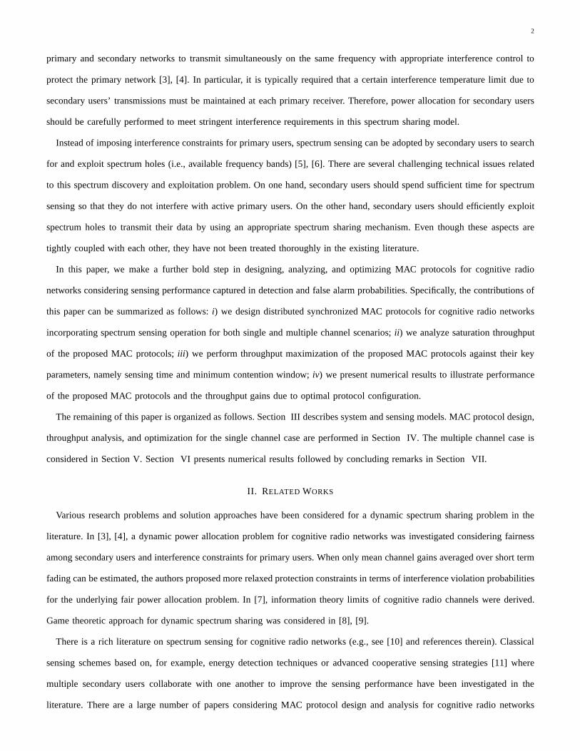
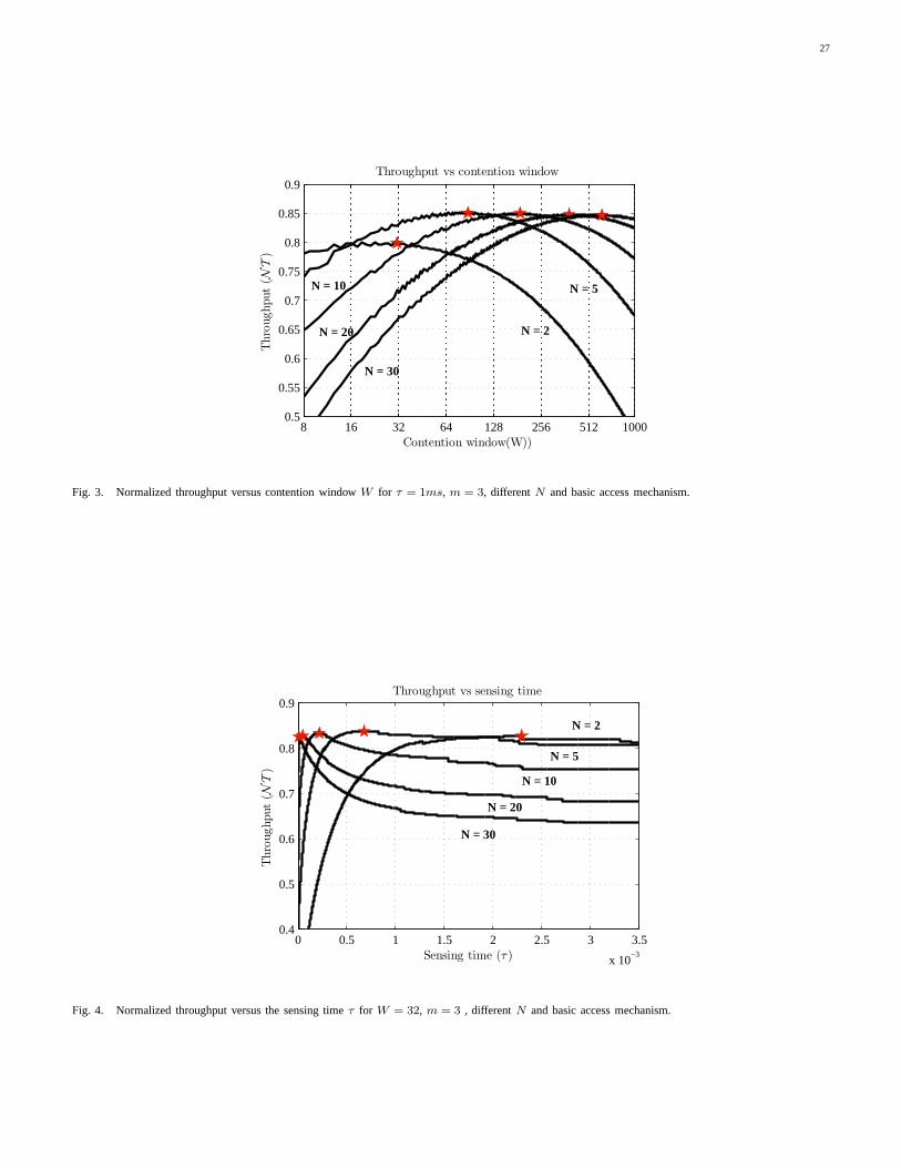
phase. The timing diagram of one particular cycle is illustrated in Fig. 2. For this single channel scenario, synchronization,

contention, and data transmission occur on the same channel.

We assume that the length of each cycle is sufficiently large so that secondary links can transmit several packets during the

data transmission phase. Indeed, the current 802.22 standard specifies the spectrum evacuation time upon the return of primary

users is 2 seconds, which is a relatively large interval. Therefore, our assumption would be valid for most practical cognitive

systems. During the data transmission phase, we assume thatactive secondary links employ a standard contention technique

to capture the channel similar to that in the CSMA/CA protocol. Exponential backoff with minimum contention windowW

and maximum backoff stagem [24] is employed in the contention phase. For brevity, we refer to W simply as contention

6

window in the following. Specifically, suppose that the current backoff stage of a particular secondary user isi then it starts

the contention by choosing a random backoff time uniformly distributed in the range[0, 2iW − 1], 0 ≤ i ≤ m. This user then

starts decrementing its backoff time counter while carriersensing transmissions from other secondary links.

Let σ denote a mini-slot interval, each of which corresponds one unit of the backoff time counter. Upon hearing a transmission

from any secondary link, each secondary link will “freeze” its backoff time counter and reactivate when the channel is sensed

idle again. Otherwise, if the backoff time counter reaches zero, the underlying secondary link wins the contention. Here, either

two-way or four-way handshake with RTS/CST will be employedto transmit one data packet on the available channel. In the

four-way handshake, the transmitter sends RTS to the receiver and waits until it successfully receives CTS before sending a

data packet. In both handshake schemes, after sending the data packet the transmitter expects an acknowledgment (ACK) from

the receiver to indicate a successful reception of the packet. Standard small intervals, namely DIFS and SIFS, are used before

backoff time decrements and ACK packet transmission as described in [24]. We refer to this two-way handshaking technique

as a basic access scheme in the following analysis.

B. Throughput Maximization

Given the sensing model and proposed MAC protocol, we are interested in finding its optimal configuration to achieve the

maximum throughput subject to protection constraints for primary receivers. Specifically, letNT (τ,W ) be the normalized

total throughput, which is a function of sensing timeτ and contention windowW . Suppose that each primary receiver requires

that detection probability achieved by its conflicting primary link i be at leastPi

d. Then, the throughput maximization problem

can be stated as follows:

Problem 1:

maxτ,W

NT (τ,W )

s.t. P id

(εi, τ

)≥ P i

d, i = 1, 2, · · · , N

0 < τ ≤ T, 0 < W ≤ Wmax,

(3)

whereWmax is the maximum contention window and recall thatT is the cycle interval. In fact, optimal sensingτ would

allocate sufficient time to protect primary receivers and optimal contention window would balance between reducing collisions

among active secondary links and limiting protocol overhead.

C. Throughput Analysis and Optimization

We perform saturation throughput analysis and solve the optimization problem (3) in this subsection. Throughput analysis

for the cognitive radio setting under investigation is moreinvolved compared to standard MAC protocol throughput analysis

(e.g., see [23], [24]) because the number of active secondary links participating in the contention in each cycle variesdepending

7

on the sensing outcomes. Suppose that all secondary links have same packet length. LetPr (n = n0) and T (τ, φ |n = n0 )

be the probability thatn0 secondary links participating in the contention and the conditional normalized throughput whenn0

secondary links join the channel contention, respectively. Then, the normalized throughput can be calculated as

NT =

N∑

n0=1

T (τ,W |n = n0 ) Pr (n = n0), (4)

where recall thatN is the number of secondary links,τ is the sensing time,W is the contention window. In the following,

we show how to calculatePr (n = n0) andT (τ, φ |n = n0 ).

1) Calculation of Pr (n = n0): It is noted that only secondary links whose sensing outcomesin the sensing phase indicate

an available channel proceed to contention in the data transmission phase. There are two scenarios for which this can happen

for a particular secondary linki:

• The primary user is not active and no false alarm is generatedby the underlying secondary link.

• The primary user is active and secondary linki mis-detects its presence.

Therefore, secondary linki joins contention in the data transmission phase with probability

P iidle =

[1− P i

f

(εi, τ

)]P i (H0) + P i

m

(εi, τ

)P i (H1) , (5)

whereP im

(εi, τ

)= 1 − P i

d

(εi, τ

)is the mis-detection probability. Otherwise, it will be silent for the whole cycle and waits

until the next cycle. This occurs with probability

P ibusy = 1− P i

idle =

= P if

(εi, τ

)P i (H0) + P i

d

(εi, τ

)P i (H1)

. (6)

We assume that interference of active primary users to the secondary user is negligible; therefore, a transmission fromany

secondary link only fails when it collides with transmissions from other secondary links. Now, letSk denote one particular

subset of all secondary links having exactlyn0 secondary links. There areCn0

N = N !n0!(N−n0)!

such setsSk. The probability of

the event thatn0 secondary links join contention in the data transmission phase can be calculated as

Pr (n = n0) =

Cn0N∑

k=1

∏

i∈Sk

P iidle

∏

j∈S\Sk

Pjbusy , (7)

whereS denotes the set of allN secondary links, andS\Sk is the complement ofSk with N − n0 secondary links. If all

secondary links have the sameSNRp and the same probabilitiesP i (H0) and P i (H1), then we haveP iidle = Pidle and

P ibusy = Pbusy = 1− Pidle for all i. In this case, (7) becomes

Pr (n = n0) = Cn0

N (1− Pbusy)n0(Pbusy)

N−n0 , (8)

where all terms in the sum of (7) become the same.

Remark 4: In general, interference from active primary users will impact transmissions of secondary users. However,

strong interference from primary users would imply high SNR of sensing signals collected at primary users. In this

8

high SNR regime, we typically require small sensing time while still satisfactorily protecting primary users. Therefore,

for the case in which interference from active primary usersto secondary users is small, sensing time will have the

most significant impact on the investigated sensing-throughput tradeoff. Therefore, consideration of this setting enables

us to gain better insight into the underlying problem. Extension to the more general case is possible by explicitly

calculating transmission rates achieved by secondary users as a function of SINR. Due to the space constraint, we will

not explore this issue further in this paper.

2) Calculation of Conditional Throughput: The conditional throughput can be calculated by using the technique developed

by Bianchi in [24] where we approximately assume a fixed transmission probabilityφ in a generic slot time. Specifically,

Bianchi shows that this transmission probability can be calculated from the following two equations [24]

φ =2 (1− 2p)

(1− 2p) (W + 1) +Wp (1− (2p)m), (9)

p = 1− (1− φ)n−1

, (10)

wherem is the maximum backoff stage,p is the conditional collision probability (i.e., the probability that a collision is observed

when a data packet is transmitted on the channel).

Suppose there aren0 secondary links participating in contention in the third phase, the probability of the event that at least

one secondary link transmits its data packet can be written as

Pt = 1− (1− φ)n0 . (11)

However, the probability that a transmission occurring on the channel is successful given there is at least one secondary link

transmitting can be written as

Ps =n0φ(1− φ)

n0−1

Pt. (12)

The average duration of a generic slot time can be calculatedas

Tsd = (1− Pt)Te + PtPsTs + Pt (1− Ps)Tc, (13)

whereTe = σ, Ts and Tc represent the duration of an empty slot, the average time thechannel is sensed busy due to a

successful transmission, and the average time the channel is sensed busy due to a collision, respectively. These quantities can

be calculated as [24]

For basic mechanism:

Ts = T 1s = H + PS + SIFS + 2PD+ACK+DIFS

Tc = T 1c = H + PS +DIFS + PD

H = HPHY +HMAC

, (14)

9

whereHPHY andHMAC are the packet headers for physical and MAC layers,PS is the packet size, which is assumed to

be fixed in this paper,PD is the propagation delay,SIFS is the length of a short interframe space,DIFS is the length of a

distributed interframe space,ACK is the length of an acknowledgment.

For RTS/CTS mechanism:

Ts = T 2s = H + PS + 3SIFS + 2PD+

RTS + CTS +ACK +DIFS

Tc = T 2c = H +DIFS +RTS + PD

, (15)

where we abuse notations by lettingRTS andCTS represent the length ofRTS andCTS control packets, respectively.

Based on these quantities, we can express the conditional normalized throughput as follows:

T (τ, φ |n = n0 ) =

⌊T − τ

Tsd

⌋ PsPtPS

T, (16)

where⌊.⌋ denotes the floor function and recall thatT is the duration of a cycle. Note that⌊T−τTsd

⌋denotes the average number

of generic slot times in one particular cycle excluding the sensing phase. Here, we omit the length of the synchronization

phase, which is assumed to be negligible.

3) Optimal Sensing and MAC Protocol Design: Now, we turn to solve the throughput maximization problem formulated

in (3). Note that we can calculate the normalized throughputgiven by (4) by usingPr (n = n0) calculated from (7) and

the conditional throughput calculated from (16). It can be observed that the detection probabilityP id

(εi, τ

)in the primary

protection constraintsP id

(εi, τ

)≥ P i

d depends on both detection thresholdεi and the optimization variableτ .

We can show that by optimizing the normalized throughput over τ andW while fixing detection thresholdsεi = εi0 where

P id

(εi0, τ

)= P i

d, i = 1, 2, · · · , N , we can achieve almost the maximum throughput gain. The intuition behind this observation

can be interpreted as follows. If we chooseεi < εi0 for a givenτ , then bothP id

(εi, τ

)andP i

f

(εi, τ

)increase compared to

the caseεi = εi0. As a result,P ibusy given in (6) increases. Moreover, it can be verified that the increase inP i

busy will lead to

the shift of the probability distributionPr (n = n0) to the left. Specifically,Pr (n = n0) given in (7) increases for smalln0

and decreases for largen0 asP ibusy increases. Fortunately, with appropriate choice of contention windowW the conditional

throughputT (τ,W |n = n0 ) given in (16) is quite flat for differentn0 (i.e., it only decreases slightly whenn0 increases).

Therefore, the normalized throughput given by (4) is almosta constant when we chooseεi < εi0.

In the following, we will optimize the normalized throughput over τ andW while choosing detection thresholds such that

P id

(εi0, τ

)= P i

d, i = 1, 2, · · · , N . From these equality constraints and (2) we have

P if = Q

(αi +

√τfsγ

i)

(17)

whereαi =√2γi + 1Q−1

(P id

). Hence, the optimization problem (3) becomes independent of all detection thresholdsεi, i =

1, 2, · · · , N . Unfortunately, this optimization problem is still a mixedinteger program (note thatW takes integer values), which

10

is difficult to solve. In fact, it can be verified even if we allow W to be a real number, the resulting optimization problem

is still not convex because the objective function is not concave [27]. Therefore, standard convex optimization techniques

cannot be employed to find the optimal solution for the optimization problem under investigation. Therefore, we have to rely

on numerical optimization [25] to find the optimal configuration for the proposed MAC protocol. Specifically, for a given

contention windowW we can find the corresponding optimal sensing timeτ as follows:

Problem 2:

max0<τ≤T

NT(τ,W ) =

N∑

n0=1

T (τ,W |n = n0 )Pr (n = n0). (18)

This optimization problem is not convex because its objective function is not concave in general. However, we will prove

thatNT(τ) is an unimodal function in the range of[0, T ]. Specifically,NT(τ) is monotonically increasing in[0, τ) while it

is monotonically decreasing in(τ , T ] for some0 < τ ≤ T . Hence,NT(τ ) is the only global maximum in the entire range of

[0, T ]. This property is formally stated in the following proposition.

Proposition 1: The objective functionNT(τ) of (18) satisfies the following properties

1) limτ→T

∂NT∂τ < 0,

2) limτ→0

∂NT∂τ = +∞,

3) there is an uniqueτ whereτ is in the range of[0, T ] such that∂NT (τ)∂τ = 0,

4) the objective functionNT(τ) is bounded from above.

Proof: The proof is provided in Appendix A.

We would like to discuss the properties stated in Proposition 1. Properties 1, 2, and 4 imply that there must be at least one

τ in [0, T ] that maximizesNT (τ). The second property implies that indeed such an optimal solution is unique. Therefore,

one can find the globally optimal(W ∗, τ∗) by finding optimalτ for eachW in its feasible range[1,Wmax]. The procedure to

find (W ∗, τ∗) can be described in Algorithm 1. Numerical studies reveal that this algorithm has quite low computation time

for practical values ofWmax andT .

Algorithm 1 OPTIMIZATION OF COGNITIVE MAC PROTOCOL

1: For each integer value ofW ∈ [1,Wmax], find the optimalτ according to (18), i.e.,

τ (W ) = argmax0<τ≤T

NT(τ,W ) (19)

2: The globally optimal(W ∗, τ∗) can then be found as

(W ∗, τ∗) = argmaxW,τ(W )

NT(τ (W ),W ). (20)

11

D. Some Practical Implementation Issues

Deployment for the optimal configuration of the proposed MAC protocol can be done as follows. Each secondary

user will need to spend some time to estimate the channel availability probabilities, channel SNRs, and the number of

secondary users sharing the underlying spectrum. When these system parameters have been estimated, each secondary

user can independently calculate the optimal sensing time and minimum contention window and implement them.

Therefore, implementation for optimal MAC protocol can be performed in a completely distributed manner, which

would be very desirable.

V. MAC D ESIGN, ANALYSIS, AND OPTIMIZATION : MULTIPLE CHANNEL CASE

We consider the MAC protocol design, analysis and optimization for the multi-channel case in this section.

A. MAC Protocol Design

We propose a synchronized multi-channel MAC protocol for dynamic spectrum sharing in this subsection. To exploit spectrum

holes in this case, we assume that there is one control channel which belongs to the secondary network (i.e., it is always available)

andM data channels which can be exploited by secondary users. We further assume that each transmitting secondary user

employ a reconfigurable transceiver which can be tuned to thecontrol channel or vacant channels for data transmission easily.

In addition, we assume that this transceiver can turn on and off the carriers on the available or busy channels, respectively

(e.g., this can be achieved by the OFDM technology).

There are still three phases for each cycle as in the single-channel case. However, in the first phase, namely the sensing

phase of lengthτ , all secondary users simultaneously perform spectrum sensing on all M underlying channels. Because the

control channel is always available, all secondary users exchange beacon signals to achieve synchronization in the second

phase. Moreover, only active secondary links whose sensingoutcomes indicate at least one vacant channel participate in the

third phase (i.e., data transmission phase). As a result, the transmitter of the winning link in the contention phase will need to

inform its receiver about the available channels. Finally,the winning secondary link will transmit data on all vacant channels

in the data transmission phase. The timing diagram of one particular cycle is illustrated in Fig. 2.

Again, we also assume that the length of each cycle is sufficiently large such that secondary links can transmit several

packets on each available channel during the data transmission phase. In the data transmission phase, we assume that active

secondary links adopt the standard contention technique tocapture the channels similar to that employed by the CSMA/CA

protocol using exponential backoff and either two-way or four-way handshake as described in Section III. For the case with

two-way handshake, both secondary transmitters and receivers need to perform spectrum sensing. With four-way handshake,

only secondary transmitters need to perform spectrum sensing and the RTS message will contain additional information about

the available channels on which the receiver will receive data packets. Also, multiple packets (i.e., one on each available

12

channel) are transmitted by the winning secondary transmitter. Finally, the ACK message will be sent by the receiver to

indicate successfully received packets on the vacant channels.

B. Throughput Maximization

In this subsection, we discuss how to find the optimal configuration to maximize the normalized throughput under sensing

constraints for primary users. Suppose that each primary receiver requires that detection probability achieved by itsconflicting

primary link i on channelj be at leastPij

d . Then, the throughput maximization problem can be stated asfollows:

Problem 3:

maxτ,W

NT (τ,W )

s.t. P ijd

(εij , τ

)≥ P ij

d , i ∈ [1, N ] , j ∈ [1,M ]

0 < τ ≤ T, 0 < W ≤ Wmax,

(21)

whereP ijd is the detection probability for secondary useri on channelj, Wmax is the maximum contention window and recall

that T is the cycle interval. We will assume that for each secondaryuseri, Pd

(εij , τ

)and P ij

d are the same for all channel

j, respectively. This would be valid because sensing performance (i.e., captured inPd

(εij , τ

)andPf

(εij , τ

)) depends on

detection thresholdsǫij and the SNRγij , which would be the same for different channelsj. In this case, the optimization

problem reduces to that of the same form as (3) although the normalized throughputNT (τ,W ) will need to be derived for

this multi-channel case. For brevity, we will drop all channel indexj in these quantities whenever possible.

C. Throughput Analysis and Optimization

We analyze the saturation throughput and show how to obtain an optimal solution forProblem 3 . Again we assume that all

secondary links transmit data packets of the same length. Let Pr (n = n0), E [l] andT (τ, φ |n = n0 ) denote the probability

that n0 secondary links participating in the contention phase, theaverage number of vacant channels at the winning SU link,

and the conditional normalized throughput whenn0 secondary links join the contention, respectively. Then, the normalized

throughput can be calculated as

NT =

N∑

n0=1

T (τ,W |n = n0 ) Pr (n = n0)E [l]

M, (22)

where recall thatN is the number of secondary links,M is the number of channels,τ is the sensing time,W is the contention

window. Note that this is the average system throughput per channel. We will calculateT (τ, φ |n = n0 ) using (16) for the

proposed MAC protocol with four-way handshake and exponential random backoff. In addition, we also show how to calculate

Pr (n = n0) .

13

1) Calculation of Pr (n = n0) and E [l]: Recall that only secondary links whose sensing outcomes indicate at least one

available channel participate in contention in the data transmission phase. Again, as in the single channel case derived in

Section IV-C1 the sensing outcome at secondary useri indicates that channelj is available or busy with probabilitiesP iidle and

P ibusy, which are in the same forms with (6) and (5), respectively (recall that we have dropped the channel indexj in these

quantities). Now,Pr (n = n0) can be calculated from these probabilities. Recall that secondary linki only joins the contention

if its sensing outcomes indicate at least one vacant channel. Otherwise, it will be silent for the whole cycle and waits until the

next cycle. This occurs if its sensing outcomes indicate that all channels are busy.

To gain insight into the optimal structure of the optimal solution while keeping mathematical details sufficiently tractable, we

will consider the homogeneous case in the following whereP if , P i

d (therefore,P iidle andP i

busy) are the same for all secondary

usersi. The obtained results, however, can extended to the generalcase even though the corresponding expressions will be

more lengthy and tedious. For the homogeneous system, we will simplify P iSUidle andP i

SUbusy to PSUidle andPSUbusy ,

respectively for brevity. Therefore, the probability thata particular channel is indicated as busy or idle by the corresponding

spectrum sensor can be written as

Pbusy = PfP (H0) + PdP (H1) , (23)

Pidle = 1− Pbusy. (24)

Let Pr (l = l0) denote the probability thatl0 out ofM channels are indicated as available by the spectrum sensors. Then, this

probability can be calculated as

Pr (l = l0) =

M

l0

P l0

idlePM−l0busy . (25)

Now, let PSUidle be the probability that a particular secondary linki participates in the contention (i.e., its spectrum sensors

indicate at least one available channel) andPSUbusy be the probability that secondary linki is silent (i.e., its spectrum sensors

indicate that all channels are busy). Then, these probabilities can be calculated as

PSUbusy = Pr (l = 0) = PMbusy, (26)

PSUidle =

M∑

l0=1

Pr (l = l0) = 1− PSUbusy . (27)

Again we assume that a transmission from a particular secondary link only fails if it collides with transmissions from other

14

secondary links. The probability thatn0 secondary links join the contention can be calculated by using (27) and (26) as follows:

Pr (n = n0) =

N

n0

Pn0

SUidlePN−n0

SUbusy

=

N

n0

(1− PM

busy

)n0

PM(N−n0)busy

. (28)

From (25), we can calculate the average number of available channels, denoted by the expectationE [l], at one particular

secondary link as

E[l] =M∑

l0=0

l0 Pr (l = l0) =M∑

l0=0

l0

M

l0

P l0

idlePM−l0busy

= MPidle = M (1− Pbusy)

. (29)

2) Optimal Sensing and MAC Protocol Design: We now tackle the throughput maximization problem formulated in (21). In

this case, the normalized throughput given by (22) can be calculated by usingPr (n = n0) in (28), the conditional throughput in

(16), and the average number of available channels in (29). Similar to the single-channel case, we will optimize the normalized

throughput overτ andW while choosing a detection threshold such thatPd (ε0, τ) = Pd. Under these equality constraints,

the false alarm probability can be written as

Pf = Q(α+

√τfsγ

)(30)

whereα =√2γ + 1Q−1

(Pd

). Hence,Problem 3 is independent of detection thresholds. Again, for a given contention window

W we can find the corresponding optimal sensing timeτ in the following optimization problem

Problem 4:

maxτ

N T (τ)∆= NT (τ,W ) |W=W

s.t. 0 ≤ τ ≤ T

. (31)

Similar to the single-channel case, we will prove thatNT (τ) is a unimodal function in the range of[0, T ]. Therefore, there

is a unique global maximum in the entire range of[0, T ]. This is indeed the result of several properties stated in the following

proposition.

Proposition 2: The functionN T (τ) satisfies the following properties

1) limτ→0

∂NT (τ)∂τ > 0,

2) limτ→T

∂NT (τ)∂τ < 0,

3) there is an uniqueτ whereτ is in the range of[0, T ] such that∂NT (τ)∂τ = 0,

4) and the objective functionNT (τ) is bounded from above.

15

Therefore, it is a unimodal function in the range of[0, T ]

Proof: The proof is provided in Appendix B.

Therefore, given one particular value ofW we can find a unique optimalτ (W ) for the optimization problem (31). Then,

we can find the globally optimal(W ∗, τ∗) by finding optimalτ for eachW in its feasible range[1,Wmax]. The procedure to

find (W ∗, τ∗) is the same as that described inAlgorithm 1 .

VI. N UMERICAL RESULTS

We present numerical results to illustrate throughput performance of the proposed cognitive MAC protocols. We take key

parameters for the MAC protocols from Table II in [24]. Otherparameters are chosen as follows: cycle time isT = 100ms;

mini-slot (i.e., generic empty slot time) isσ = 20µs; sampling frequency for spectrum sensing isfs = 6MHz; bandwidth of

PUs’ QPSK signals is6MHz. In addition, the exponential backoff mechanism with the maximum backoff stagem is employed

to reduce collisions.

A. Performance of Single Channel MAC Protocol

For the results in this section, we choose other parameters of the cognitive network as follows. The signal-to-noise ratio of

PU signals at secondary linksSNRip are chosen randomly in the range[−15,−20]dB. The target detection probability for

secondary links and the probabilitiesP i (H0) are chosen randomly in the intervals[0.7, 0.9] and [0.7, 0.8], respectively. The

basic scheme is used as a handshaking mechanism for the MAC protocol.

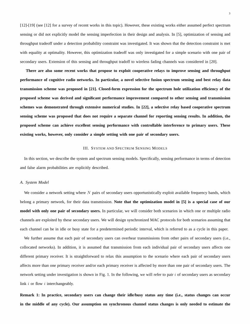
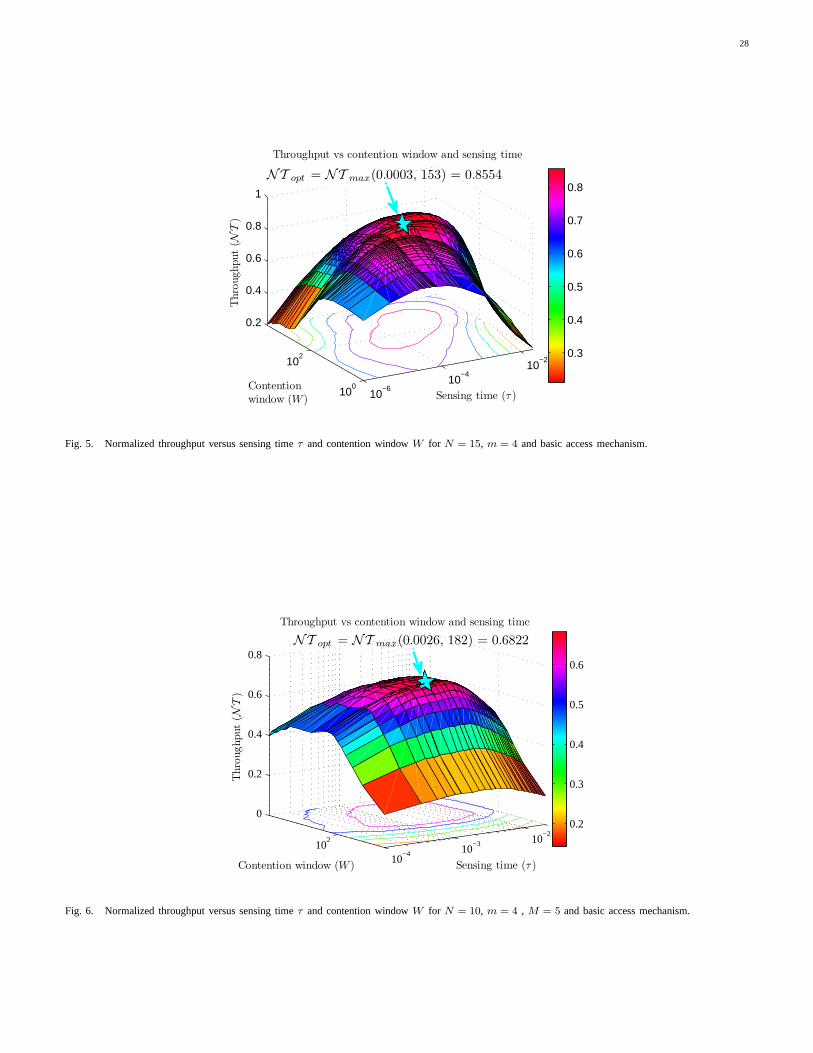
In Fig. 3, we show the normalized throughputNT versus contention windowW for different values ofN when the sensing

time is fixed atτ = 1ms and the maximum backoff stage is chosen atm = 3 for one particular realization of system parameters.

The maximum throughput on each curve is indicated by a star symbol. This figure indicates that the maximum throughput is

achieved at largerW for largerN . This is expected because larger contention window can alleviate collisions among active

secondary for larger number of secondary links. It is interesting to observe that the maximum throughput can be larger than

0.8 althoughP i (H0) are chosen in the range[0.7, 0.8]. This is due to a multiuser gain because secondary links are in conflict

with difference primary receivers.

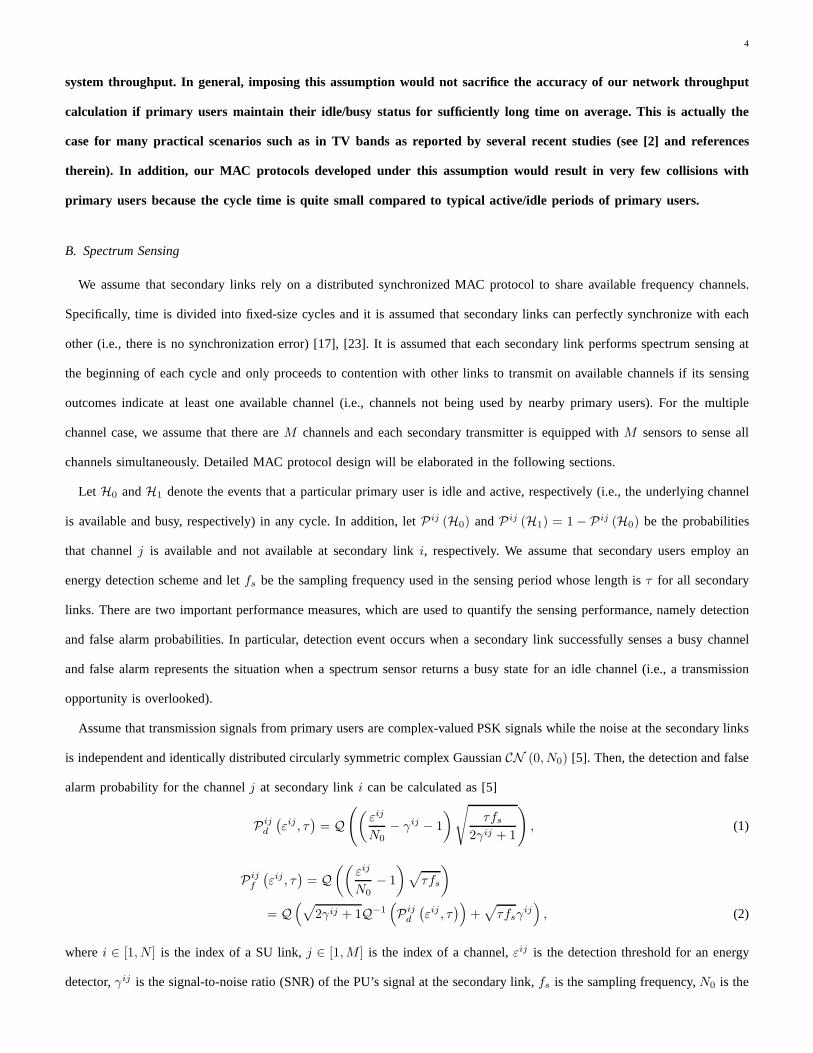
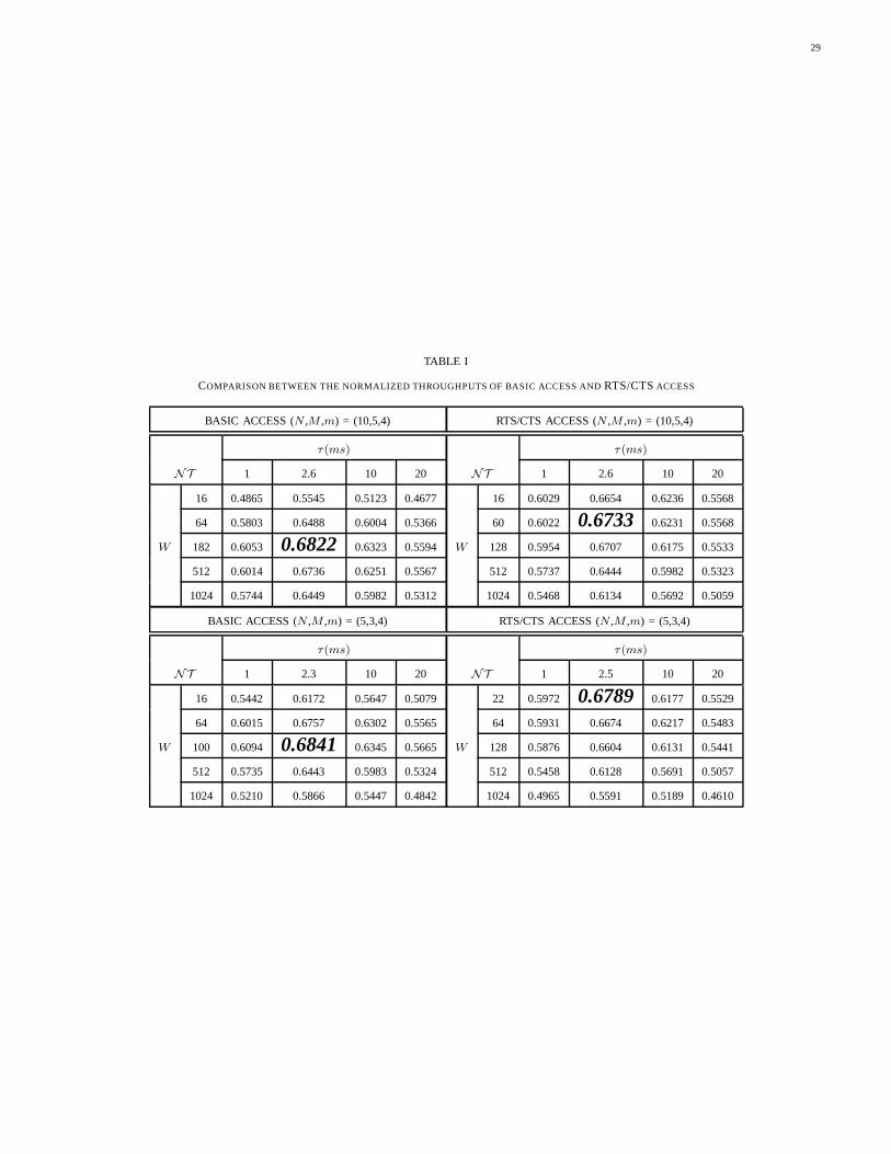
In Fig. 4 we present the normalized throughputNT versus sensing timeτ for a fixed contention windowW = 32, maximum

backoff stagem = 3, and different number of secondary linksN . The maximum throughput is indicated by a star symbol on

each curve. This figure confirms that the normalized throughput NT increases whenτ is small and decreases with largeτ as

being proved in Proposition 1. Moreover, for a fixed contention window the optimal sensing time indeed decreases with the

number of secondary linksN . Finally, the multi-user diversity gain can also be observed in this figure.

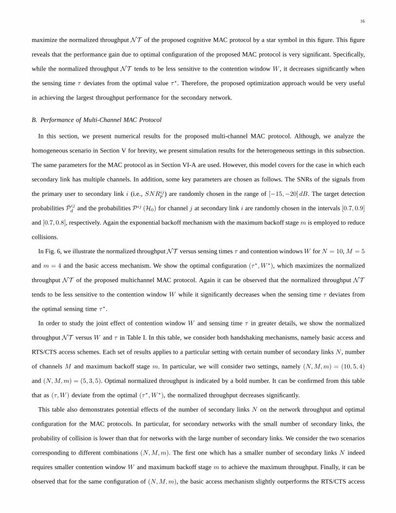
To illustrate the joint effects of contention windowW and sensing timeτ , we show the normalized throughputNT versus

τ and contention windowW for N = 15 andm = 4 in Fig. 5. We show the globally optimal parameters(φ∗, τ∗) which

16

maximize the normalized throughputNT of the proposed cognitive MAC protocol by a star symbol in this figure. This figure

reveals that the performance gain due to optimal configuration of the proposed MAC protocol is very significant. Specifically,

while the normalized throughputNT tends to be less sensitive to the contention windowW , it decreases significantly when

the sensing timeτ deviates from the optimal valueτ∗. Therefore, the proposed optimization approach would be very useful

in achieving the largest throughput performance for the secondary network.

B. Performance of Multi-Channel MAC Protocol

In this section, we present numerical results for the proposed multi-channel MAC protocol. Although, we analyze the

homogeneous scenario in Section V for brevity, we present simulation results for the heterogeneous settings in this subsection.

The same parameters for the MAC protocol as in Section VI-A are used. However, this model covers for the case in which each

secondary link has multiple channels. In addition, some keyparameters are chosen as follows. The SNRs of the signals from

the primary user to secondary linki (i.e., SNRijp ) are randomly chosen in the range of[−15,−20]dB. The target detection

probabilitiesP ijd and the probabilitiesP ij (H0) for channelj at secondary linki are randomly chosen in the intervals[0.7, 0.9]

and[0.7, 0.8], respectively. Again the exponential backoff mechanism with the maximum backoff stagem is employed to reduce

collisions.

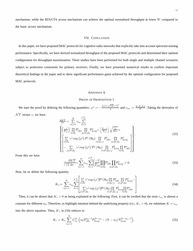
In Fig. 6, we illustrate the normalized throughputNT versus sensing timesτ and contention windowsW for N = 10, M = 5

andm = 4 and the basic access mechanism. We show the optimal configuration (τ∗,W ∗), which maximizes the normalized

throughputNT of the proposed multichannel MAC protocol. Again it can be observed that the normalized throughputNT

tends to be less sensitive to the contention windowW while it significantly decreases when the sensing timeτ deviates from

the optimal sensing timeτ∗.

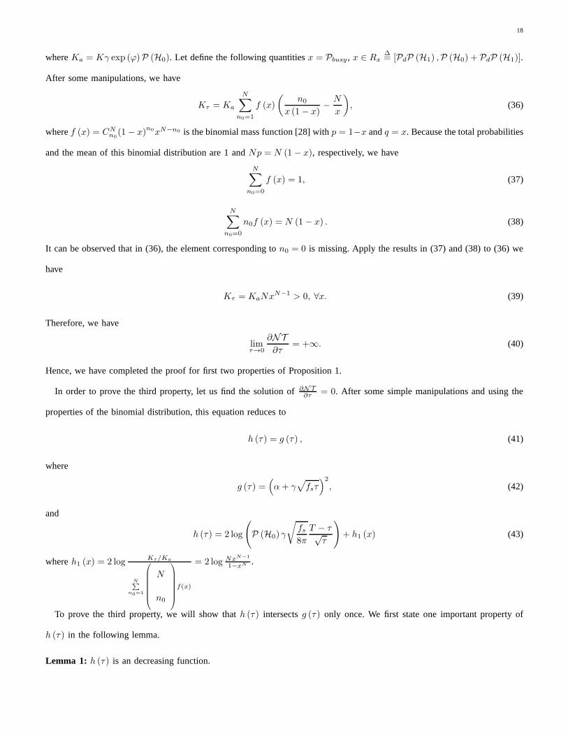
In order to study the joint effect of contention windowW and sensing timeτ in greater details, we show the normalized

throughputNT versusW andτ in Table I. In this table, we consider both handshaking mechanisms, namely basic access and

RTS/CTS access schemes. Each set of results applies to a particular setting with certain number of secondary linksN , number

of channelsM and maximum backoff stagem. In particular, we will consider two settings, namely(N,M,m) = (10, 5, 4)

and(N,M,m) = (5, 3, 5). Optimal normalized throughput is indicated by a bold number. It can be confirmed from this table

that as(τ,W ) deviate from the optimal(τ∗,W ∗), the normalized throughput decreases significantly.

This table also demonstrates potential effects of the number of secondary linksN on the network throughput and optimal

configuration for the MAC protocols. In particular, for secondary networks with the small number of secondary links, the

probability of collision is lower than that for networks with the large number of secondary links. We consider the two scenarios

corresponding to different combinations(N,M,m). The first one which has a smaller number of secondary linksN indeed

requires smaller contention windowW and maximum backoff stagem to achieve the maximum throughput. Finally, it can be

observed that for the same configuration of(N,M,m), the basic access mechanism slightly outperforms the RTS/CTS access

17

mechanism, while the RTS/CTS access mechanism can achieve the optimal normalized throughput at lowerW compared to

the basic access mechanism.

VII. C ONCLUSION

In this paper, we have proposed MAC protocols for cognitive radio networks that explicitly take into account spectrum sensing

performance. Specifically, we have derived normalized throughput of the proposed MAC protocols and determined their optimal

configuration for throughput maximization. These studies have been performed for both single and multiple channel scenarios

subject to protection constraints for primary receivers. Finally, we have presented numerical results to confirm important

theoretical findings in the paper and to show significant performance gains achieved by the optimal configuration for proposed

MAC protocols.

APPENDIX A

PROOF OFPROPOSITION1

We start the proof by defining the following quantities:ϕj := − (αj+√τfsγ

j)2

2 andcn0 := PsPtPST . Taking the derivative of

NT versusτ , we have

∂NT∂τ =

N∑n0=1

cn0

CNn0∑

k=1

(−1Tsd

) ∏i∈Sk

P iidle

∏j∈S\Sk

Pjbusy+

⌊T−τTsd

⌋√fs8πτ×

∑i∈Sk

γi exp(ϕi)P i (H0)

∏l∈Sk\i

P lidle

∏j∈S\Sk

Pjbusy

− ∑j∈S\Sk

γj exp(ϕj)Pj (H0)

∏l∈S\Sk\j

P lbusy

∏i∈Sk

P iidle

. (32)

From this we have

limτ→T

∂NT∂τ

=

N∑

n0=1

cn0

CNn0∑

k=1

(−1

Tsd

)∏

i∈Sk

P iidle

∏

j∈S\Sk

Pjbusy < 0. (33)

Now, let us define the following quantity

Kτ:=N∑

n0=1

cn0

CNn0∑

k=1

∑i∈Sk

γi exp(ϕi)P i(H0)

∏l∈Sk\i

P lidle

∏j∈S\Sk

Pjbusy−

∑j∈S\Sk

γj exp(ϕj)Pj(H0)

∏l∈S\Sk\j

P lbusy

∏i∈Sk

P iidle

. (34)

Then, it can be shown thatKτ > 0 as being explained in the following. First, it can be verifiedthat the termcn0 is almost a

constant for differentn0. Therefore, to highlight intuition behind the underlying property (i.e.,Kτ > 0), we substituteK = cn0

into the above equation. Then,Kτ in (34) reduces to

Kτ = Ka

N∑

n0=1

CNn0

(n0Pn0−1

idle PN−n0

busy − (N − n0)PN−n0−1busy

), (35)

18

whereKa = Kγ exp (ϕ)P (H0). Let define the following quantitiesx = Pbusy , x ∈ Rx∆= [PdP (H1) ,P (H0) + PdP (H1)].

After some manipulations, we have

Kτ = Ka

N∑

n0=1

f (x)

(n0

x (1− x)− N

x

), (36)

wheref (x) = CNn0(1− x)n0xN−n0 is the binomial mass function [28] withp = 1−x andq = x. Because the total probabilities

and the mean of this binomial distribution are 1 andNp = N (1− x), respectively, we have

N∑

n0=0

f (x) = 1, (37)

N∑

n0=0

n0f (x) = N (1− x) . (38)

It can be observed that in (36), the element corresponding ton0 = 0 is missing. Apply the results in (37) and (38) to (36) we

have

Kτ = KaNxN−1 > 0, ∀x. (39)

Therefore, we have

limτ→0

∂NT∂τ

= +∞. (40)

Hence, we have completed the proof for first two properties ofProposition 1.

In order to prove the third property, let us find the solution of ∂NT∂τ = 0. After some simple manipulations and using the

properties of the binomial distribution, this equation reduces to

h (τ) = g (τ) , (41)

where

g (τ) =(α+ γ

√fsτ)2

, (42)

and

h (τ) = 2 log

(P (H0) γ

√fs8π

T − τ√τ

)+ h1 (x) (43)

whereh1 (x) = 2 log Kτ/Ka

N∑n0=1

N

n0

f(x)

= 2 log NxN−1

1−xN .

To prove the third property, we will show thath (τ) intersectsg (τ) only once. We first state one important property of

h (τ) in the following lemma.

Lemma 1: h (τ) is an decreasing function.

19

Proof: Taking the first derivative ofh(.), we have

∂h

∂τ=

−1

τ− 2

T − τ+

∂h1

∂x

∂x

∂τ. (44)

We now derive∂x∂τ and ∂h1

∂x as follows:

∂x

∂τ= −P (H0) γ

√fs8πτ

exp

(−(α+ γ

√fsτ)2

2

)< 0, (45)

∂h1

∂x= 2

N − 1 + xN

x (1− xN )> 0. (46)

Hence, ∂h1

∂x∂x∂τ < 0. Using this result in (44), we have∂h∂τ < 0. Therefore, we can conclude thath (τ) is monotonically

decreasing.

We now consider functiong (τ). Take the derivative ofg (τ), we have

∂g

∂τ=(α+ γ

√fsτ) γ

√fs√τ

. (47)

Therefore, the monotonicity property ofg (τ) only depends ony = α+ γ√fsτ . Properties 1 and 2 imply that there must be

at least one intersection betweenh (τ) and g (τ). We now prove that there is indeed a unique intersection. To proceed, we

consider two different regions forτ as follows:

Ω1 =τ∣∣α+ γ

√fsτ < 0, τ ≤ T

=0 < τ < α2

γ2fs

and

Ω2 =τ∣∣α+ γ

√fsτ ≥ 0, τ ≤ T

=

α2

γ2fs≤ τ ≤ T

.

From the definitions of these two regions, we haveg (τ) decreases inΩ1 and increases inΩ2. To show that there is a unique

intersection betweenh (τ) andg (τ), we prove the following.

Lemma 2: The following statements are correct:

1) If there are intersections betweenh (τ) and g (τ) in Ω2 then it is the only intersection in this region and there is no

intersection inΩ1.

2) If there are intersections betweenh (τ) and g (τ) in Ω1 then it is the only intersection in this region and there is no

intersection inΩ2.

Proof: We prove the first statement now. Recall thatg (τ) monotonically increases inΩ2; therefore,g (τ) andh (τ) can

intersect at most once in this region (becauseh (τ) decreases). In addition,g (τ) andh (τ) cannot intersection inΩ1 for this

case if we can prove that∂h∂τ < ∂g∂τ . This is because both functions decrease inΩ1. We will prove that∂h∂τ < ∂g

∂τ in lemma 3

after this proof.

We now prove the second statement of lemma 2. Recall that we have ∂h∂τ < ∂g

∂τ . Therefore, there is at most one intersection

betweeng (τ) andh (τ) in Ω1. In addition, it is clear that there cannot be any intersection between these two functions inΩ2

for this case.

20

Lemma 3: We have∂h∂τ < ∂g

∂τ .

Proof: From (44), we can see that lemma 3 holds if we can prove the following stronger result

−1

τ+

∂h1

∂τ<

∂g

∂τ, (48)

where ∂h1

∂τ = ∂h1

∂x∂x∂τ , ∂x

∂τ is derived in (45),∂h1

∂x is derived in (46) and∂g∂τ is given in (47).

To prove (48), we will prove the following

− 1

τ+

yP (H0) γ√

fsτ

P (H0) +√2πP (H1)

(1− Pd

)(−y) exp

(y2

2

) <∂g

∂τ, (49)

wherey =(α+ γ

√fsτ < 0

). Then, we show that

∂h1

∂τ<

yP (H0) γ√

fsτ

P (H0) +√2πP (H1)

(1− Pd

)(−y) exp

(y2

2

) . (50)

Therefore, the result in (48) will hold. Let us prove (50) first. First, let us prove the following

∂h1

∂x>

2

1− x. (51)

Using the result in∂h1

∂x from (46), (51) is equivalent to

2N − 1 + xN

x (1− xN )>

2

1− x, (52)

After some manipulations, we get

(1− x)(N − 1−

(x+ x2 + · · ·+ xN−1

))> 0. (53)

It can be observed that0 < x < 1 and 0 < xi < 1, i ∈ [1, N − 1]. So N − 1 −(x+ x2 + · · ·+ x(N−1)

)> 0; hence (53)

holds. Therefore, we have completed the proof for (51).

We now show that the following inequality holds

2

1− x>

2√2π (−y) exp

(y2

2

)

P (H0) +√2πP (H1)

(1− Pd

)(−y) exp

(y2

2

) . (54)

This can be proved as follows. In [26], it has been shown thatQ (t) with t > 0 satisfies

1

Q (t)>

√2πt exp

(t2

2

). (55)

Apply this result toPf = Q (y) = 1−Q (−y) with y =(α+ γ

√fsτ)< 0 we have

1

1− Pf>

√2π (−y) exp

(y2

2

). (56)

After some manipulations, we obtain

Pf > 1− 1√2π (−y) exp

(y2

2

) . (57)

21

Recall that we have definedx = PfP (H0) + PdP (H1). Using the result in (57), we can obtain the lower bound of21−x

given in (54). Using the results in (51) and (54), and the factthat ∂x∂τ < 0, we finally complete the proof for (50).

To complete the proof of the lemma, we need to prove that (49) holds. Substitute∂g∂τ from (47) to (49) and make some

further manipulations, we have

1

−y (y − α)> 1−

yP (H0) γ√

fsτ

P (H0) +√2πP (H1)

(1− Pd

)(−y) exp

(y2

2

) . (58)

Let us consider the LHS of (58). We have0 < y − α = γ√fsτ < −α; therefore, we have0 < −y < −α. Apply the

CauchySchwarz inequality to−y andy − α, we have the following

0 < −y (y − α) ≤(−y + y − α

2

)2

=α2

4. (59)

Hence

1

−y (y − α)≥ 4

α2=

4

(2γ + 1)(Q−1

(Pd

))2 > 1. (60)

It can be observed that the RHS of (58) is less than 1. Therefore, (58) holds, which implies that (49) and (48) also hold.

Finally, the last property holds because becausePr (n = n0) < 1 and conditional throughput are all bounded from above.

Therefore, we have completed the proof of Proposition 1.

APPENDIX B

PROOF OFPROPOSITION2

To prove the properties stated in Proposition 2, we first find the derivative ofN T (τ). Again, it can be verified thatPtPsPST

is almost a constant for differentn0. To demonstrate the proof for the proposition, we substitute this term as a constant value,

denoted asK, in the throughput formula. In addition, for largeT ,⌊T−τTsd

⌋is very close toT−τ

Tsd. Therefore,N T can be

accurately approximated as

N T(τ)=N∑

n0=1

K

N

n0

(T − τ )

(1− xM

)n0xM(N−n0) (1− x), (61)

whereK = PtPsPST , andx = Pbusy . Now, let us define the following function

f ′ (x) =(1− xM

)n0xM(N−n0) (1− x) . (62)

Then, we have

∂f ′

∂x= f ′ (x)

[ −1

1− x− Mn0

1− xMxM−1 +

M (N − n0)

x

], (63)

22

and ∂x∂τ is the same as (45). Hence, the first derivation ofNT (τ) can be written as

∂NT (τ)∂τ =

N∑n0=1

K

N

n0

[−f ′ (x) + (T − τ) ∂f ′

∂x∂x∂τ

]

=N∑

n0=1K

N

n0

f ′ (x)×

(T − τ)[

11−x + Mn0

1−xM xM−1 − M(N−n0)x

]

×P (H0) γ√

fs8πτ exp

(− (α+γ

√fsτ)

2

2

)− 1

. (64)

From (23), the range ofx, namelyRx can be expressed as[PdP (H1) , P (H0) + PdP (H1)]. Now, it can be observed that

limτ→T

∂N T (τ)

∂τ= −

N∑

n0=1

K

N

n0

f ′ (x) < 0. (65)

Therefore, the second property of Proposition 2 holds.

Now, let us define the following quantity

K′τ =

N∑

n0=1

N

n0

f

′ (x)

[1

1− x+

Mn0

1− xMxM−1−M(N− n0)

x

]. (66)

Then, it can be seen thatlimτ→0

∂NT (τ)∂τ = +∞ > 0 if K′

τ > 0, ∀M, N, x ∈ Rx. This last property is stated and proved in the

following lemma.

Lemma 4: K′τ > 0, ∀M, N, x ∈ Rx.

Proof: Making some manipulations to (66), we have

K′τ =

(1− (1−x)M

x

) N∑n0=1

N

n0

(1− xM

)n0xM(N−n0)+

M(1−x)x(1−xM)

N∑n0=1

N

n0

n0

(1− xM

)n0xM(N−n0).

(67)

It can be observed thatN∑

n0=1

N

n0

(1− xM

)n0xM(N−n0) and

N∑n0=1

N

n0

n0

(1− xM

)n0xM(N−n0) represent a cumu-

lative distribution function (CDF) and the mean of a binomial distribution [28] with parameterp, respectively missing the term

corresponding ton0 = 0 wherep = 1−xM . Note that the CDF and mean of such a distribution are 1 andNp = N(1− xM

),

respectively. Hence, (67) can be rewritten as

K ′τ =

(1− (1− x)M

x

)(1− xMN

)+

M (1− x)

x (1− xM )N(1− xM

). (68)

23

After some manipulations, we have

K′τ = 1− xMN +MNxMN−1 (1− x) > 0, ∀x. (69)

Therefore, we have completed the proof.

Hence, the first property of Proposition 1 also holds.

To prove the third property, let us consider the following equation ∂NT (τ)∂τ = 0. After some manipulations, we have the

following equivalent equation

g (τ) = h′ (τ) , (70)

where

g (τ) =(α+ γ

√fsτ)2

, (71)

h′ (τ) = 2 log

(P (H0) γ

√fs8π

T − τ√τ

)+ h′

1 (x) , (72)

h′1 (x) = 2 log

K ′τ

N∑n0=1

N

n0

f ′ (x)

, (73)

K ′τ is given in (66). We have the following result forh′ (τ).

Lemma 5: h′ (τ) monotonically decreases inτ .

Proof: The derivative ofh′ (τ) can be written as

∂h′

∂τ=

−1

τ− 2

T − τ+

∂h′1

∂τ. (74)

In the following, we will show that∂h′

1

∂x > 0 for all x ∈ Rx, all M andN , and ∂x∂τ < 0. Hence ∂h′

1

∂τ =∂h′

1

∂x∂x∂τ < 0. From

this, we have∂h′

∂τ < 0; therefore, the property stated in lemma 5 holds.

We now show that∂h′

1

∂x > 0 for all x ∈ Rx, all M andN . SubstituteK′τ in (69) to (73) and exploit the property of the

CDF of the binomial distribution function, we have

h′1 (x) = 2 log 1−xMN+MNxMN−1(1−x)

(1−x)N∑

n0=1

N

n0

(1−xM )n0xM(N−n0)

= 2 log 1−xMN+MNxMN−1(1−x)(1−x)(1−xMN )

. (75)

Taking the first derivative ofh′1 (x) and performing some manipulations, we obtain

∂h′1

∂x= 2

r (r − 1)xr−2(1− x)2(1− xr)

+(1− xr)2+ r2x2(r−1)(1− x)

2

(1− xr + rx(r−1) (1− x)

)(1− x) (1− xr)

, (76)

24

wherer = MN . It can be observed that there is no negative term in (76); hence, ∂h′

1

∂x > 0 for all x ∈ Rx, all M andN .

Therefore, we have proved the lemma.

To prove the third property, we show thatg (τ) andh′ (τ) intersect only once in the range of[0, T ]. This will be done using

the same approach as that in Appendix A. Specifically, we willconsider two regionsΩ1 andΩ2 and prove two properties

stated in Lemma 2 for this case. As in Appendix A, the third property holds if we can prove− 1τ +

∂h′

1

∂τ < ∂g∂τ . It can be

observed that all steps used to prove this inequality are thesame as those in the proof of (48) for Proposition 1. Hence, we

need to prove

∂h′1

∂x>

2

1− x. (77)

Substitute∂h′

1

∂x from (76) to (77), this inequality reduces to

2

r (r − 1)xr−2(1− x)2 (1− xr)

+(1− xr)2+ r2x2(r−1)(1− x)

2

(1− xr + rx(r−1) (1− x)

)(1− x) (1− xr)

>2

1− x. (78)

After some manipulations, this inequality becomes equivalent to

rx(r−2) (1− x)2[r −

(1 + x+ x2 + · · ·+ x(r−1)

)]> 0. (79)

It can be observed that0 < x < 1 and0 < xi < 1, i ∈ [0, r − 1]. Hence, we haver−(1 + x+ x2 + · · ·+ x(r−1)

)> 0 which

shows that (79) indeed holds. Therefore, (77) holds and we have completed the proof of the third property. Finally, the last

property of the Proposition is obviously correct. Hence, wehave completed the proof of Proposition 2.

REFERENCES

[1] Q. Zhao and B.M. Sadler, “A Survey of dynamic spectrum access,” IEEE Signal Processing Mag., vol. 24, no. 3, pp. 79-89, May, 2007.

[2] C. Stevenson, G. Chouinard, L. Zhongding, H. Wendong, S.Shellhammer, W. Caldwell, “IEEE 802.22: The first cognitiveradio wireless regional area

network standard,”IEEE Commun. Mag., vol. 47, no. 1, pp. 130–138, Jan. 2009.

[3] D. I. Kim, L. B. Le, and E. Hossain, “Joint rate and power allocation for cognitive radios in dynamic spectrum access environment,” IEEE Trans.

Wireless Commun., vol. 7, no. 12, pp. 5517-5527, Dec. 2008.

[4] L. B. Le and E. Hossain, “Resource allocation for spectrum underlay in cognitive radio networks,”IEEE Trans. Wireless Commun., vol. 7, no. 12, pp.

5306-5315, Dec. 2008.

[5] L. Ying-Chang, Z. Yonghong, E. C. Y. Peh and H. Anh Tuan, “Sensing-throughput tradeoff for cognitive radio networks”, IEEE Trans. Wireless Commun.,

vol. 7, no. 4, pp. 1326-1337, April 2008.

[6] E. C. Y. Peh, Y.-C. Liang and Y. L. Guan, “Optimization of cooperative sensing in cognitive radio networks: A sensing-throughput tradeoff view”, in

Proc. IEEE International Conf. Commun., pp. 3521-3525, 2009.

[7] N. Devroye, P. Mitran, and V. Tarokh, “Achievable rates in cognitive radio channels,”IEEE Trans. Inf. Theory, vol. 52, no. 5, pp. 1813–1827, May 2006.

[8] F. Wang, M. Krunz, and S. Cui, “Price-based spectrum management in cognitive radio networks,”IEEE J. Sel. Topics Signal Processing, vol. 2, no. 1,

pp. 74–87, Feb. 2008.

25

[9] D. Niyato and E. Hossain, “Competitive pricing for spectrum sharing in cognitive radio networks: Dynamic game, inefficiency of Nash equilibrium, and

collusion,” IEEE J. Sel. Areas Commun., vol. 26, no. 1, pp. 192–202, Jan. 2008.

[10] T. Yucek and H. Arslan, “A survey of spectrum sensing algorithms for cognitive radio applications,”IEE Commun. Surveys and Tutorials, vol. 11, no.

1, pp. 116–130, 2009.

[11] J. Unnikrishnan and V. V. Veeravalli, “Cooperative sensing for primary detection in cognitive radio,”IEEE J. Sel. Areas Signal Processing, vol. 2, no.

1, pp. 18–27, Feb. 2008.

[12] C. Cormiob and K. R. Chowdhurya, “A survey on MAC protocols for cognitive radio networks,”Elsevier Ad Hoc Networks, vol. 7, no. 7, pp. 1315-1329,

Sept. 2009.

[13] H. Kim and K. G. Shin, “Efficient discovery of spectrum opportunities with MAC-layer sensing in cognitive radio networks,” IEEE Trans. Mobile

Computing, vol. 7, no. 5, pp. 533-545, May 2008.

[14] H. Su and X. Zhang, “Opportunistic MAC protocols for cognitive radio based wireless networks,” inProc. CISS’2007.

[15] H. Nan, T.-I. Hyon, and S.-J. Yoo, “Distributed coordinated spectrum sharing MAC protocol for cognitive radio,” inIEEE DySPAN’2007.

[16] C. Cordeiro, and K. Challapali, “ C-MAC: A cognitive MACprotocol for multi-channel wireless networks,” inIEEE DySPAN’2007.

[17] Y.R. Kondareddy, and P. Agrawal, “Synchronized MAC protocol for multi-hop cognitive radio networks,” inProc. IEEE ICC’2008.

[18] A. C.-C. Hsu, D.S.L. Weit, and C.-C.J. Kuo, “A cognitiveMAC protocol using statistical channel allocation for wireless ad-hoc networks,” inProc.

IEEE WCNC’2007.

[19] H. Su, and X. Zhang, “Cross-layer based opportunistic MAC protocols for QoS provisionings over cognitive radio wireless networks,”IEEE J. Sel.

Areas Commun., vol. 26, no. 1, pp. 118–129, Jan. 2008.

[20] Y. Zuo, Y.-D. Yao, and B. Zheng, “Outage probability analysis of cognitive transmissions: Impact of spectrum sensing overhead,”IEEE Trans. Wireless

Commun., vol. 9, no. 8, pp. 2676–2688, Aug. 2010.

[21] Y. Zou, Y.-D. Yao, and B. Zheng, “Cognitive transmissions with multiple relays in cognitive radio networks,”IEEE Trans. Wireless Commun., vol. 10,

no. 2, pp. 648–659, Feb. 2011.

[22] Y. Zou, Y.-D. Yao, and B. Zheng, “A selective-relay based cooperative spectrum sensing scheme without dedicated reporting channels in cognitive radio

networks,” IEEE Trans. Wireless Commun., vol. 10, no. 4, pp. 1188–1198, April 2011.

[23] J. Shi, E. Aryafar, T. Salonidis and E. W. Knightly, “Synchronized CSMA contention: Model, implementation and evaluation”, in Proc. IEEE INFOCOM,

pp. 2052-2060, 2009.

[24] G. Bianchi, “Performance analysis of the ieee 802.11 distributed coordination function,”IEEE J. Sel. Areas Commun., vol. 18, no. 3, pp. 535-547 Mar.

2000.

[25] S. Kameshwaran and Y. Narahari, “Nonconvex piecewise linear knapsack problems,”European J. Operational Research, vol. 192, no. 1, pp. 56-68,

2009.

[26] George K. Karagiannidis and Athanasios S. Lioumpas, “An improved approximation for the Gaussian Q-function,”IEEE Commun. Let., vol. 11, no. 8,

pp. 644-646, Aug. 2007.

[27] S. P. Boyd and L. Vandenberghe, Convex Optimization, Cambridge University Press, Cambridge, UK ; New York, 2004.

[28] V. Krishnan, Probability and Random Processes, Wiley-Interscience, 2006, p. xiii, 723 p.

26

Fig. 1. Considered network and spectrum sharing model (PU: primary user, SU: secondary user)

One cycle

timeSensing SYN

DATA Contention DATA

. . .

CTSRTS

DIFSSIFS SIFS

Backoff RTS/CTS exchange

DATADATADC1

DC2

DATADATADC3 . . .

Not used

PU occupancy

CC: Control channel

DATA ACK

SIFS

. . .

. . .

. . .

time

time

time

CC

DC: Data channel

Contention

Fig. 2. Timing diagram of the proposed multi-channel MAC protocol.

27

8 16 32 64 128 256 512 10000.5

0.55

0.6

0.65

0.7

0.75

0.8

0.85

0.9

Contention window(W))

Thro

ughput

(NT

)

Throughput vs contention window

N = 5

N = 20

N = 10

N = 30

N = 2

Fig. 3. Normalized throughput versus contention windowW for τ = 1ms, m = 3, differentN and basic access mechanism.

0 0.5 1 1.5 2 2.5 3 3.5

x 10−3

0.4

0.5

0.6

0.7

0.8

0.9

Sensing time (τ )

Thro

ughput

(NT

)

Throughput vs sensing time

N = 30

N = 20

N = 10

N = 5

N = 2

Fig. 4. Normalized throughput versus the sensing timeτ for W = 32, m = 3 , different N and basic access mechanism.

28

10−6

10−4

10−2

100

102

0.2

0.4

0.6

0.8

1

Sensing time (τ )

Throughput vs contention window and sensing time

Contentionwindow (W)

Thro

ughput

(NT

)

0.3

0.4

0.5

0.6

0.7

0.8NT opt = NT max(0.0003, 153) = 0.8554

Fig. 5. Normalized throughput versus sensing timeτ and contention windowW for N = 15, m = 4 and basic access mechanism.

10−4 10

−3 10−2

102

0

0.2

0.4

0.6

0.8

Sensing time (τ )

Throughput vs contention window and sensing time

Contention window (W)

Thro

ughput

(NT

)

0.2

0.3

0.4

0.5

0.6

NT opt = NT max(0.0026, 182) = 0.6822

Fig. 6. Normalized throughput versus sensing timeτ and contention windowW for N = 10, m = 4 , M = 5 and basic access mechanism.

29

TABLE I

COMPARISON BETWEEN THE NORMALIZED THROUGHPUTS OF BASIC ACCESS AND RTS/CTSACCESS

BASIC ACCESS (N ,M ,m) = (10,5,4)

τ(ms)

NT 1 2.6 10 20

16 0.4865 0.5545 0.5123 0.4677

64 0.5803 0.6488 0.6004 0.5366

W 182 0.6053 0.6822 0.6323 0.5594

512 0.6014 0.6736 0.6251 0.5567

1024 0.5744 0.6449 0.5982 0.5312

RTS/CTS ACCESS (N ,M ,m) = (10,5,4)

τ(ms)

NT 1 2.6 10 20

16 0.6029 0.6654 0.6236 0.5568

60 0.6022 0.6733 0.6231 0.5568

W 128 0.5954 0.6707 0.6175 0.5533

512 0.5737 0.6444 0.5982 0.5323

1024 0.5468 0.6134 0.5692 0.5059

BASIC ACCESS (N ,M ,m) = (5,3,4)

τ(ms)

NT 1 2.3 10 20

16 0.5442 0.6172 0.5647 0.5079

64 0.6015 0.6757 0.6302 0.5565

W 100 0.6094 0.6841 0.6345 0.5665

512 0.5735 0.6443 0.5983 0.5324

1024 0.5210 0.5866 0.5447 0.4842

RTS/CTS ACCESS (N ,M ,m) = (5,3,4)

τ(ms)

NT 1 2.5 10 20

22 0.5972 0.6789 0.6177 0.5529

64 0.5931 0.6674 0.6217 0.5483

W 128 0.5876 0.6604 0.6131 0.5441

512 0.5458 0.6128 0.5691 0.5057

1024 0.4965 0.5591 0.5189 0.4610