Physics 125Course Notes

Angular Momentum040429 F. Porter

1 Introduction

This note constitutes a discussion of angular momentum in quantum mechan-ics. Several results are obtained, important to understanding how to solveproblems involving rotational symmetries in quantum mechanics. We will of-ten give only partial proofs to the theorems, with the intent that the readercomplete them as necessary. In the hopes that this will prove to be a usefulreference, the discussion is rather more extensive than usually encounteredin quantum mechanics textbooks.

2 Rotations: Conventions and Parameteriza-

tions

A rotation by angle θ about an axis e (passing through the origin in R3)is denoted by Re(θ). We’ll denote an abstract rotation simply as R. It isconsidered to be “positive” if it is performed in a clockwise sense as we lookalong e. As with other transformations, our convention is that we think of arotation as a transformation of the state of a physical system, and not as achange of coordinate system (sometimes referred to as the “active view”). IfRe(θ) acts on a configuration of points (“system”) we obtain a new, rotated,configuration: If x is a point of the old configuration, and x′ is its imageunder the rotation, then:

x′ = Re(θ)x. (1)

That is, R is a linear transformation described by a 3×3 real matrix, relativeto a basis (e1, e2, e3).

Geometrically, we may observe that:

Re(−θ) = R−1e (θ), (2)

I = Re(0) = Re(2πn), n = integer, (3)

Re(θ)Re(θ′) = Re(θ + θ′), (4)

Re(θ + 2πn) = Re(θ), n = integer, (5)

R−e = Re(−θ). (6)1

A product of the form Re(θ)Re′(θ′) means “first do Re′(θ

′), then do Re(θ)to the result”. All of these identities may be understood in terms of ma-trix identities, in addition to geometrically. Note further that the set of allrotations about a fixed axis e forms a one-parameter abelian group.

It is useful to include in our discussion of rotations the notion also ofreflections: We’ll denote the space reflection with respect to the origin by P ,for parity:

Px = −x. (7)

Reflection in a plane through the origin is called a mirroring. Let e be a unitnormal to the mirror plane. Then

Mex = x − 2e(e · x), (8)

since the component of the vector in the plane remains the same, and thenormal component is reversed.

Theorem: 1.

[P,Re(θ)] = 0. (9)

[P,Me] = 0. (10)

(The proof of this is trivial, since P = −I.)2.

PMe = MeP = Re(π). (11)

3. P , Me, and Re(π) are “involutions”, that is:

P 2 = I. (12)

M2e = I. (13)

[Re(π)]2 = I. (14)

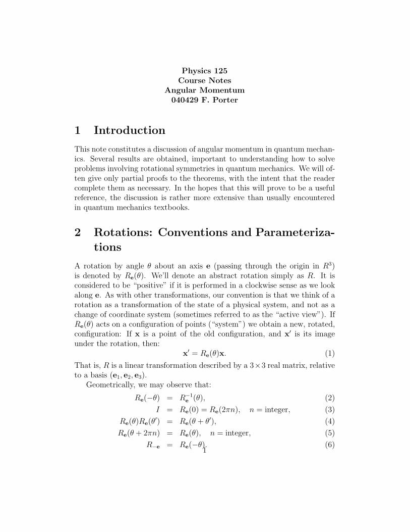
Theorem: Let Re(θ) be a rotation and let e′, e′′ be two unit vectors per-pendicular to unit vector e such that e′′ is obtained from e′ accordingto:

e′′ = Re(θ/2)e′. (15)

ThenRe(θ) = Me′′Me′ = Re′′(π)Re′(π). (16)

Hence, every rotation is a product of two mirrorings, and also a productof two rotations by π.

2

M

M

x

R

e'

e'' e

a+b=a

b

e'

e''

/2

/2/2

e( )θθ

θ

θθ

x

Figure 1: Proof of the theorem that a rotation about e by angle θ is equivalentto the product of two mirrorings or rotations by π.

Proof: We make a graphical proof, referring to Fig. 1.

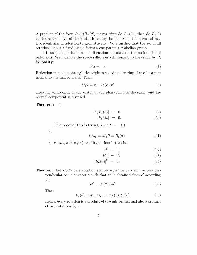
Theorem: Consider the spherical triangle in Fig. 2.

1. We haveRe3(2α3)Re2(2α2)Re1(2α1) = I, (17)

where the unit vectors ei are as labelled in the figure.

2. Hence, the product of two rotations is a rotation:

Re2(2α2)Re1(2α1) = Re3(−2α3). (18)

The set of all rotations is a group, where group multiplication isapplication of successive rotations.

Proof: Use the figure and label M1 the mirror plane spanned by e2, e3, etc.Then we have:

Re1(2α1) = M3M2

Re2(2α2) = M1M3

Re3(2α3) = M2M1. (19)

3

Μ1

Μ 2

Μ 3

α

αα

e

e

e

3

2

1

.

.

.Figure 2: Illustration for theorem. Spherical triangle vertices are defined asthe intersections of unit vectors e1, e2, e3 on the surface of the unit sphere.

Thus,

Re3(2α3)Re2(2α2)Re1(2α1) = (M2M1)(M1M3)(M3M2) = I. (20)

The combination of two rotations may thus be expressed as a problemin spherical trigonometry.

As a corollary to this theorem, we have the following generalization ofthe addition formula for tangents:

Theorem: If Re(θ) = Re′′(θ′′)Re′(θ

′), and defining:

τττ = e tan θ/2

τττ ′ = e′ tan θ′/2

τττ ′′ = e′′ tan θ′′/2, (21)

then

τττ =τττ ′ + τττ ′′ + τττ ′′ × τττ ′

1 − τττ ′ · τττ ′′. (22)

This will be left as an exercise for the reader to prove.

4

Theorem: The most general mapping x → x′ of R3 into itself, such thatthe origin is mapped into the origin, and such that all distances arepreserved, is a linear, real orthogonal transformation Q:

x′ = Qx, where QTQ = I, and Q∗ = Q. (23)

Hence,x′ · y′ = x · y ∀ pointsx,y ∈ R3. (24)

For such a mapping, either:

1. det(Q) = 1, Q is called a proper orthogonal transformation, andis in fact a rotation. In this case,

x′ × y′ = (x × y)′ ∀ pointsx,y ∈ R3. (25)

or,

2. det(Q) = −1, Q is called an improper orthogonal transforma-tion, and is the product of a reflection (parity) and a rotation. Inthis case,

x′ × y′ = −(x × y)′ ∀ pointsx,y ∈ R3. (26)

The set of all orthogonal transformations on three dimensions forms agroup (denoted O(3)), and the set of all proper orthogonal transforma-tions forms a subgroup (O+(3) or SO(3) of O(3)), in 1 : 1 correspon-dence with, hence a “representation” of, the set of all rotations.

Proof of this theorem will be left to the reader.

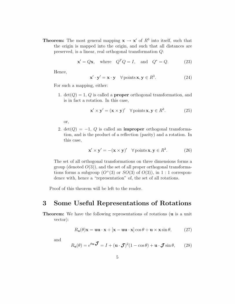
3 Some Useful Representations of Rotations

Theorem: We have the following representations of rotations (u is a unitvector):

Ru(θ)x = uu · x + [x − uu · x] cos θ + u × x sin θ, (27)

andRu(θ) = eθu·JJJ = I + (u · JJJ )2(1 − cos θ) + u · JJJ sin θ, (28)

5

where JJJ = (J1,J2,J3) with:

J1 =

0 0 00 0 −10 1 0

, J2 =

0 0 10 0 0−1 0 0

, J3 =

0 −1 01 0 00 0 0

.

(29)

Proof: The first relation may be seen by geometric inspection: It is a de-composition of the rotated vector into components along the axis ofrotation, and the two orthogonal directions perpendicular to the axisof rotation.

The second relation may be demonstrated by noticing that Jix = ei×x,where e1, e2, e3 are the three basis unit vectors. Thus,

(u · JJJ )x = u × x, (30)

and(u · JJJ )2x = u × (u × x) = u(u · x) − x. (31)

Further,

(u · JJJ )2n+m = (−)n(u · JJJ )m, n = 1, 2, . . . ; m = 1, 2. (32)

The second relation then follows from the first.

Note that

Tr [Ru(θ)] = Tr[I + (u · JJJ )2(1 − cos θ)

]. (33)

With

J 21 =

0 0 00 −1 00 0 −1

,J 2

2 =

−1 0 00 0 00 0 −1

,J 2

3 =

−1 0 00 −1 00 0 0

, (34)

we haveTr [Ru(θ)] = 3 − 2(1 − cos θ) = 1 + 2 cos θ. (35)

This is in agreement with the eigenvalues of Ru(θ) being 1, eiθ, e−iθ.

6

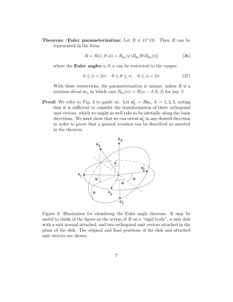
Theorem: (Euler parameterization) Let R ∈ O+(3). Then R can berepresented in the form:

R = R(ψ, θ, φ) = Re3(ψ)Re2(θ)Re3(φ), (36)

where the Euler angles ψ, θ, φ can be restricted to the ranges:

0 ≤ ψ < 2π; 0 ≤ θ ≤ π; 0 ≤ φ < 2π. (37)

With these restrictions, the parameterization is unique, unless R is arotation about e3, in which case Re3(α) = R(α− β, 0, β) for any β.

Proof: We refer to Fig. 3 to guide us. Let e′k = Rek, k = 1, 2, 3, noting

that it is sufficient to consider the transformation of three orthogonalunit vectors, which we might as well take to be intitially along the basisdirections. We must show that we can orient e′

k in any desired directionin order to prove that a general rotation can be described as assertedin the theorem.

ee

33'

e1

e2

e1'

e2'

θ

θ

ψψ φ

Figure 3: Illustration for visualizing the Euler angle theorem. It may beuseful to think of the figure as the action of R on a “rigid body”, a unit diskwith a unit normal attached, and two orthogonal unit vectors attached in theplane of the disk. The original and final positions of the disk and attachedunit vectors are shown.

7

We note that e′3 does not depend on φ since this first rotation is about

e3 itself. The polar angles of e′3 are given precisely by θ and ψ. Hence

θ and ψ are uniquely determined (within the specified ranges, andup to the ambiguous case mentioned in the theorem) by e′

3 = Re3,which can be specified to any desired orientation. The angle φ is thendetermined uniquely by the orientation of the pair (e′

1, e′2) in the plane

perpendicular to e′3.

We note that the rotation group [O+(3)] is a group of infinite order (or, isan “infinite group”, for short). There are also an infinite number of subgroupsof O+(3), including both finite and infinite subgroups. Some of the importantfinite subgroups may be classified as:

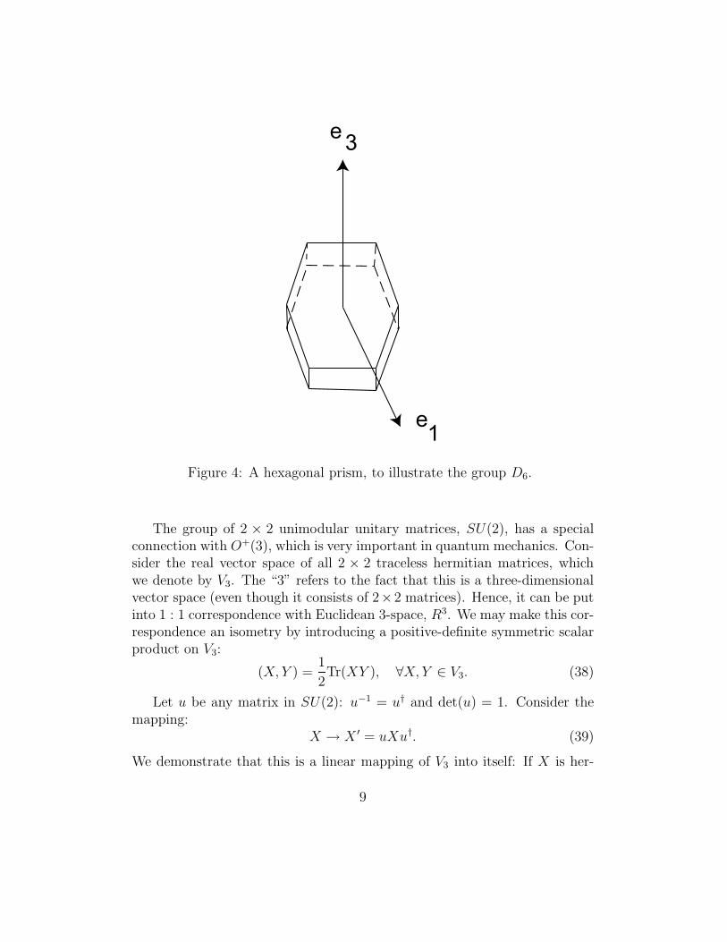
1. The Dihedral groups, Dn, corresponding to the proper symmetries ofan n-gonal prism. For example, D6 ⊂ O+(3) is the group of rotationswhich leaves a hexagonal prism invariant. This is a group of order 12,generated by rotations Re3(2π/6) and Re2(π).

2. The symmetry groups of the regular solids:

(a) The symmetry group of the tetrahedron.

(b) The symmetry group of the octahedron, or its “dual” (replacevertices by faces, faces by vertices) the cube.

(c) The symmetry group of the icosahedron, or its dual, the dodeca-hedron.

We note that the tetrahedron is self-dual.

An example of an infinite subgroup of O+(3) is D∞, the set of all rotationswhich leaves a circular disk invariant, that is, including all rotations aboutthe normal to the disk, and rotations by π about any axis in the plane of thedisk.

4 Special Unitary Groups

The set of all n × n unitary matrices forms a group (under normal matrixmultiplication), denoted by U(n). U(n) includes as a subgroup, the set ofall n × n unitary matrices with determinant equal to 1 (“unimodular”, or“special”. This subgroup is denoted by SU(n), for “Special Unitary” group.

8

e

e

3

1

Figure 4: A hexagonal prism, to illustrate the group D6.

The group of 2 × 2 unimodular unitary matrices, SU(2), has a specialconnection with O+(3), which is very important in quantum mechanics. Con-sider the real vector space of all 2 × 2 traceless hermitian matrices, whichwe denote by V3. The “3” refers to the fact that this is a three-dimensionalvector space (even though it consists of 2×2 matrices). Hence, it can be putinto 1 : 1 correspondence with Euclidean 3-space, R3. We may make this cor-respondence an isometry by introducing a positive-definite symmetric scalarproduct on V3:

(X, Y ) =1

2Tr(XY ), ∀X, Y ∈ V3. (38)

Let u be any matrix in SU(2): u−1 = u† and det(u) = 1. Consider themapping:

X → X ′ = uXu†. (39)

We demonstrate that this is a linear mapping of V3 into itself: If X is her-

9

mitian, so is X ′. If X is traceless then so is X ′:

Tr(X ′) = Tr(uXu†) = Tr(Xuu†) = Tr(X). (40)

This mapping of V3 into itself also preserves the norms, and hence, the scalarproducts:

(X ′, X ′) =1

2Tr(X ′X ′)

=1

2Tr(uXu†uXu†)

= (X,X). (41)

The mapping is therefore a rotation acting on V3 and we find that to everyelement of SU(2) there corresponds a rotation.

Let us make this notion of a connection more explicit, by picking anorthonormal basis (σ1, σ2, σ3) of V3, in the form of the Pauli matrices:

σ1 =(

0 11 0

), σ2 =

(0 −ii 0

), σ3 =

(1 00 −1

). (42)

Note that the Pauli matrices form an orthonormal basis:

1

2Tr(σασβ) = δαβ. (43)

We have the products:

σ1σ2 = iσ3, σ2σ3 = iσ1, σ3σ1 = iσ2. (44)

Different Pauli matrices anti-commute:

σα, σβ ≡ σασβ + σβσα = 2δαβI (45)

The commutation relations are:

[σα, σβ] = 2iεαβγσγ . (46)

Any element of V3 may be written in the form:

X = x · σσσ =3∑

i=1

xiσi, (47)

10

where x ∈ R3. This establishes a 1 : 1 correspondence between elements ofV3 and R3. We note that

1

2Tr [(a · σσσ)(b · σσσ)] = a · b, (48)

and

(a · σσσ)(b · σσσ) =3∑

i=1

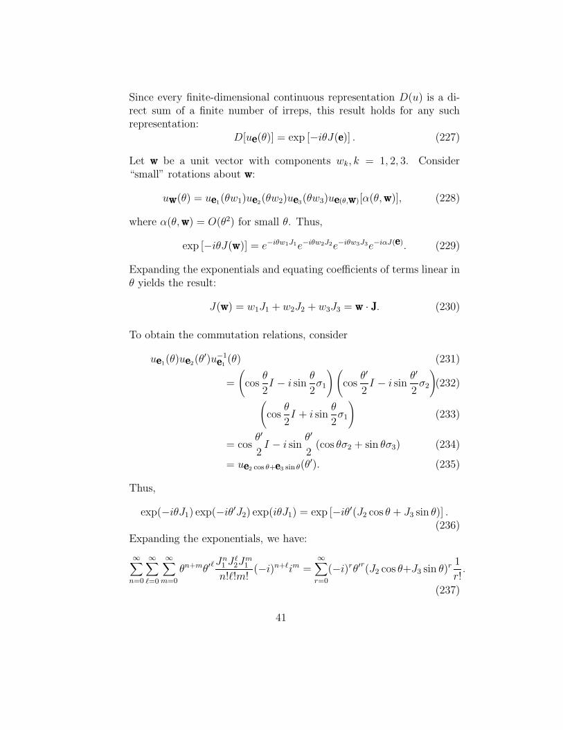
aibiσ2i +

3∑

i=1

∑

j 6=iaibjσiσj

= (a · b)I + i(a × b) · σσσ. (49)

Finally, we may see that the mapping is isometric:

(X, Y ) =1

2Tr(XY ) =

1

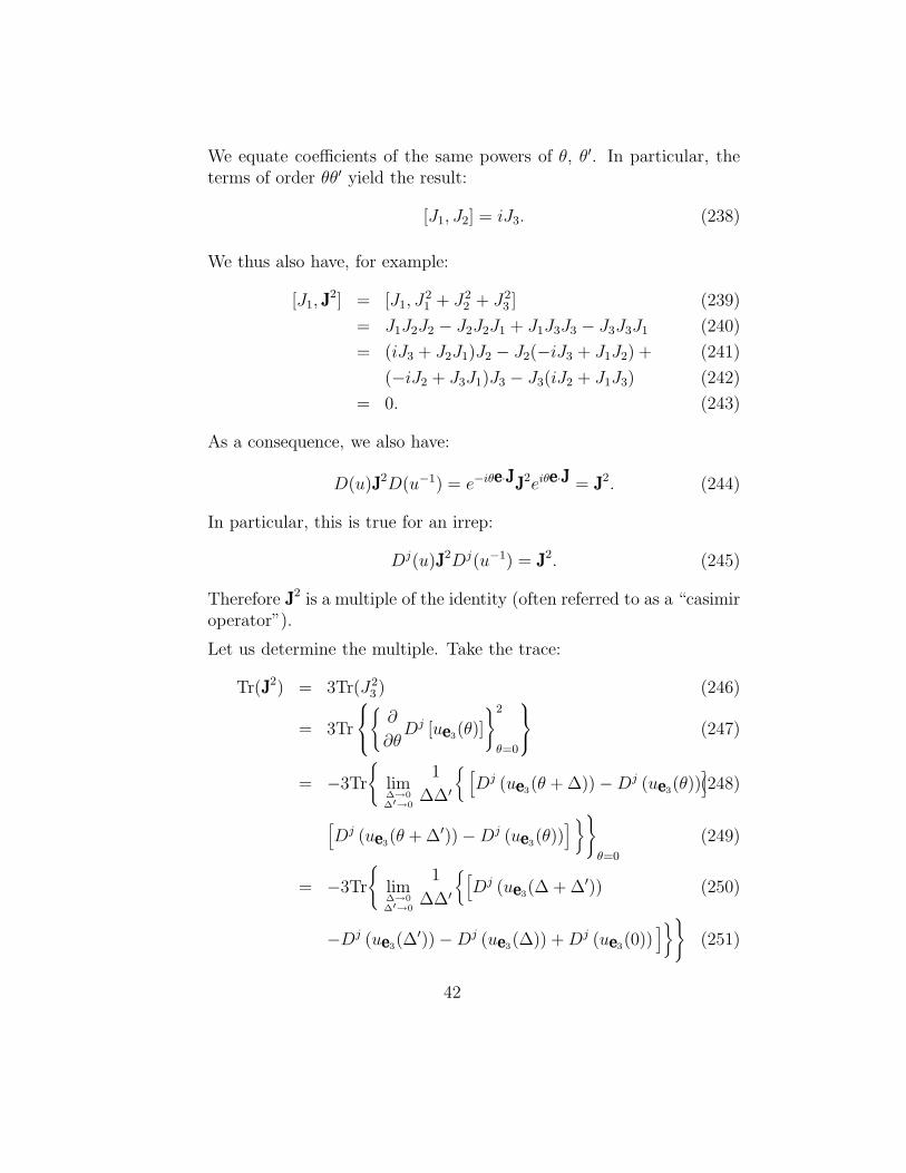
2Tr [(x · σσσ)(y · σσσ)] = x · y. (50)

Let’s investigate SU(2) further, and see the relevance of V3: Every unitarymatrix can be expressed as the exponential of a skew-hermitian (A† = −A)matrix. If the unitary matrix is also unimodular, then the skew-hermitianmatrix can be selected to be traceless. Hence, every u ∈ SU(2) is of the formu = e−iH , where H = H† and Tr(H) = 0. For every real unit vector e andevery real θ, we define ue(θ) ∈ SU(2) by:

u(θ) = exp(− i

2θe · σσσ

). (51)

Any element of SU(2) can be expressed in this form, since every tracelesshermitian matrix is a (real) linear combination of the Pauli matrices.

Now let us relate ue(θ) to the rotation Re(θ):

Theorem: Let x ∈ R3, and X = x · σσσ. Let

u(θ) = exp(− i

2θe · σσσ

), (52)

and letue(θ)Xu

†e(θ) = X ′ = x′ · σσσ. (53)

Thenx′ = Re(θ)x. (54)

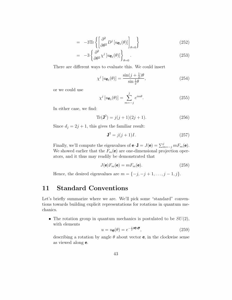
11

Proof: Note that

ue(θ) = exp(− i

2θe · σσσ

)= I cos

θ

2− i(e · σσσ) sin

θ

2. (55)

This may be demonstrated by using the identity (a · σσσ)(b · σσσ) = (a ·b)I + (a × b) · σσσ, and letting a = b = e to get (e · σ)2 = I, and usingthis to sum the exponential series.

Thus,

x′ · σσσ = ue(θ)Xu†e(θ)

=

[I cos

θ

2− i(e · σσσ) sin

θ

2

](x · σσσ)

[I cos

θ

2+ i(e · σσσ) sin

θ

2

]

= x · σ cos2 θ

2+ (e · σσσ)(x · σσσ)(e · σσσ) sin2 θ

2

+ [−i(e · σσσ)(x · σσσ) + i(x · σσσ)(e · σσσ)] sinθ

2cos

θ

2. (56)

But

(e · σσσ)(x · σσσ) = (e · x)I + i(e × x) · σσσ (57)

(x · σσσ)(e · σσσ) = (e · x)I − i(e × x) · σσσ (58)

(e · σσσ)(x · σσσ)(e · σσσ) = (e · x)(e · σ) + i [(e × x) · σσσ] (e · σσσ)

= (e · x)(e · σσσ) + i2 [(e × x) × e] · σσσ= 2(e · x)(e · σσσ) − x · σσσ, (59)

where we have made use of the identity (C × B) × A = B(A · C) −C(A · B) to obtain (e × x) × e = x − e(e · x). Hence,

x′ · σσσ =

cos2 θ

2x + sin2 θ

2[2(e · x)e − x]

· σσσ

+i sinθ

2cos

θ

2[−2i(e × x) · σσσ] . (60)

Equating coefficients of σ we obtain:

x′ = x cos2 θ

2+ [2(e · x)e − x] sin2 θ

2+ 2(e × x) sin

θ

2cos

θ

2= (e · x)e + [x − (e · x)e] cos θ + (e × x) sin θ

= Re(θ)x. (61)

12

Thus, we have shown that to every rotation Re(θ) corresponds at leastone u ∈ SU(2), and also to every element of SU(2) there corresponds arotation. We may restate the theorem just proved in the alternative form:

uXu† = u(x · σσσ)u† = x · (uσσσu†)= x · σσσ = [Re(θ)x] · σ = x ·

[R−1

e (θ)σσσ]. (62)

But x is arbitrary, souσσσu† = R−1

e (θ)σσσ, (63)

or,u−1σσσu = Re(θ)σσσ. (64)

More explicitly, this means:

u−1σiu =3∑

j=1

Re(θ)ijσj. (65)

There remains the question of uniqueness: Suppose u1 ∈ SU(2) andu2 ∈ SU(2) are such that

u1Xu†1 = u2Xu

†2, ∀X ∈ V3. (66)

Then u−12 u1 commutes with every X ∈ V3 and therefore this matrix must

be a multiple of the identity (left for the reader to prove). Since it is uni-tary and unimodular, it must equal I or −I. Thus, there is a two-to-onecorrespondence between SU(2) and O+(3): To every rotation Re(θ) corre-sponds the pair ue(θ) and −ue(θ) = ue(θ + 2π). Such a mapping of SU(2)onto O+(3) is called a homomorphism (alternatively called an unfaithfulrepresentation).

We make this correspondence precise in the following:

Theorem: 1. There is a two-to-one correspondence between SU(2) andO+(3) under the mapping:

u→ R(u), where Rij(u) =1

2Tr(u†σiuσj), (67)

and the rotation Re(θ) corresponds to the pair:

Re(θ) ↔ ue(θ),−ue(θ) = ue(θ + 2π). (68)

13

2. In particular, the pair of elements I,−I ⊂ SU(2) maps to I ∈O+(3).

3. This mapping is a homomorphism: u→ R(u) is a representationof SU(2), such that

R(u′u′′) = R(u′)R(u′′), ∀u′, u′′ ∈ SU(2). (69)

That is, the “multiplication table” is preserved under the map-ping.

Proof: 1. We have

u−1σiu =3∑

j=1

Re(θ)ijσj. (70)

Multiply by σk and take the trace:

Tr(u−1σiuσk) = Tr

3∑

j=1

Re(θ)ijσjσk

, (71)

or

Tr(u†σiuσk) =3∑

j=1

Re(θ)ijTr(σjσk). (72)

But 12Tr(σjσk) = δjk, hence

Rik(u) = Re(θ)ik =1

2Tr(u†σiuσk). (73)

Proof of the remaining statements is left to the reader.

A couple of comments may be helpful here:

1. Why did we restrict u to be unimodular? That is, why are we consider-ing SU(2), and not U(2). In fact, we could have considered U(2), butthe larger group only adds unnecessary complication. All U(2) adds ismultiplication by an overall phase factor, and this has no effect in thetransformation:

X → X ′ = uXu†. (74)

This would enlarge the two-to-one mapping to infinity-to-one, appar-ently without achieving anything of interest. So, we keep things assimple as we can make them.

14

2. Having said that, can we make things even simpler? That is, can weimpose additional restrictions to eliminate the “double-valuedness” inthe above theorem? The answer is no – SU(2) has no subgroup whichis isomorphic with O+3.

5 Lie Groups: O+(3) and SU(2)

Def: An abstract n-dimensional Lie algebra is an n-dimensional vectorspace V on which is defined the notion of a product of two vectors (∗)with the properties (x, y, z ∈ V, c a complex number):

1. Closure: x ∗ y ∈ V.

2. Distributivity:

x ∗ (y + z) = x ∗ y + x ∗ z (75)

(y + z) ∗ x = y ∗ x+ z ∗ x. (76)

3. Associativity with respect to multiplication by a complex number:

(cx) ∗ y = c(x ∗ y). (77)

4. Anti-commutativity:x ∗ y = −y ∗ x (78)

5. Non-associative (“Jacobi identity”):

x ∗ (y ∗ z) + z ∗ (x ∗ y) + y ∗ (z ∗ x) = 0 (79)

We are especially interested here in Lie algebras realized in terms of matri-ces (in fact, every finite-dimensional Lie algebra has a faithful representationin terms of finite-dimensional matrices):

Def: A Lie algebra of matrices is a vector space M of matrices which isclosed under the operation of forming the commutator:

[M ′,M ′′] = M ′M ′′ −M ′′M ′ ∈ M, ∀M ′,M ′′ ∈ M. (80)

Thus, the Lie product is the commutator: M ′ ∗M ′′ = [M ′,M ′′]. Thevector space may be over the real or complex fields.

15

Let’s look at a couple of relevant examples:

1. The set of all real skew-symmetric 3×3 matrices is a three-dimensionalLie algebra. Any such matrix is a real linear combination of the matri-ces

J1 =

0 0 00 0 −10 1 0

, J2 =

0 0 10 0 0−1 0 0

, J3 =

0 −1 01 0 00 0 0

(81)as defined already earlier. The basis vectors satisfy the commutationrelations:

[Ji,Jj] = εijkJk. (82)

We say that this Lie algebra is the Lie algebra associated with thegroup O+(3). Recall that

Ru(θ) = eθu·JJJ . (83)

2. The set of all 2×2 skew-hermitian matrices is a Lie algebra of matrices.This is also 3-dimensional, and if we write:

Sj =i

2σj, j = 1, 2, 3, (84)

we find S satisfy the “same” commutation relations as J :

[Si,Sj] = εijkSk. (85)

This is the Lie algebra associated with the group SU(2). Recall that

ue(θ) = eθe·(−i2σσσ) = eθe·SSS . (86)

This is also a real Lie algebra, i.e., a vector space over the real field,even though the matrices are not in general real.

We see that the Lie algebras of O+(3) and SU(2) have the same “struc-ture”, i.e., a 1 : 1 correspondence can be established between them which islinear and preserves all commutators. As Lie algrebras, the two are isomor-phic.

We explore a bit more the connection between Lie algebras and Liegroups. Let M be an n-dimensional Lie algebra of matrices. Associated

16

with M there is an n-dimensional Lie group G of matrices: G is the matrixgroup generated by all matrices of the form eX , where X ∈ M. We seethat O+(3) and SU(2) are Lie groups of this kind – in fact, every elementof either of these groups corresponds to an exponential of an element of theappropriate Lie algrebra.1

6 Continuity Structure

As a finite dimensional vector space, M has a continuity structure in theusual sense (i.e., it is a topological space with the “usual” topology). Thisinduces a continuity structure (topology) on G (for O+(3) and SU(2), thereis nothing mysterious about this, but we’ll keep our discussion a bit moregeneral for a while). G is an n-dimensional manifold (a topological spacesuch that every point has a neighborhood which can be mapped homeo-morphically onto n-dimensional Euclidean space). The structure of G (itsmultiplication table) in some neighborhood of the identity is uniquely deter-mined by the structure of the Lie algebra M. This statement follows fromthe Campbell-Baker-Hausdorff theorem for matrices: If matrices X, Y aresufficiently “small”, then eXeY = eZ , where Z is a matrix in the Lie algebragenerated by matrices X and Y . That is, Z is a series of repeated commu-tators of the matrices X and Y . Thus, we have the notion that the localstructure of G is determined solely by the structure of M as a Lie algebra.

We saw that the Lie algebras of O+(3) and SU(2) are isomorphic, hencethe group O+(3) is locally isomorphic with SU(2). Note, on the other hand,that the properties

(u · J )3 = −(u · J ) and (u · J )2n+m = (−)n(u · J )m, (87)

for all positive integers n,m, are not shared by the Pauli matrices, whichinstead satisfy:

(u · σ)3 = u · σ. (88)

Such algebraic properties are outside the realm of Lie algebras (the productsbeing taken are not Lie products). We also see that (as with O+(3) and

1This latter fact is not a general feature of Lie groups: To say that G is generatedby matrices of the form eX means that G is the intersection of all matrix groups whichcontain all matrices eX where X ∈ M. An element of G may not be of the form eX .

17

SU(2)) it is possible for two Lie algebras to have the same local structure,while not being globally isomorphic.

A theorem describing this general situation is the following:

Theorem: (and definition) To every Lie algebra M corresponds a uniquesimply-connected Lie group, called the Universal Covering Group,defined by M. Denote this group by GU . Every other Lie group witha Lie algebra isomorphic with M is then isomorphic with the quotientgroup of GU relative to some discrete (central – all elements whichmap to the identity) subgroup of GU iself. If the other group is simplyconnected, it is isomorphic with GU itself.

We apply this to rotations: The group SU(2) is the universal coveringgroup defined by the Lie algebra of the rotation group, hence SU(2) takeson special significance. We note that SU(2) can be parameterized as thesurface of a unit sphere in four dimensions, hence is simply connected (allclosed loops may be continuously collapsed to a point). On the other hand,O+(3) is isomorphic with the quotient group SU(2)/I(2), where I(2) is theinversion group in two dimensions:

I(2) =(

1 00 1

),(−1 0

0 −1

). (89)

7 The Haar Integral

We shall find it desirable to have the ability to perform an “invariant inte-gral” on the manifolds O+(3) and SU(2), which in some sense assigns anequal “weight” to every element of the group. The goal is to find a way ofdemocratically “averaging” over the elements of a group. For a finite group,the correspondence is to a sum over the group elements, with the same weightfor each element.

For the rotation group, let us denote the desired “volume element” byd(R). We must find an expression for d(R) in terms of the parameterization,for some parameterization of O+(3). For example, we consider the Eulerangle parameterization. Recall, in terms of Euler angles the representationof a rotation as:

R = R(ψ, θ, φ) = Re3(ψ)Re2(θ)Re3(φ). (90)

18

We will argue that the appropriate volume element must be of the form:

d(R) = Kdψ sin θdθdφ, K > 0. (91)

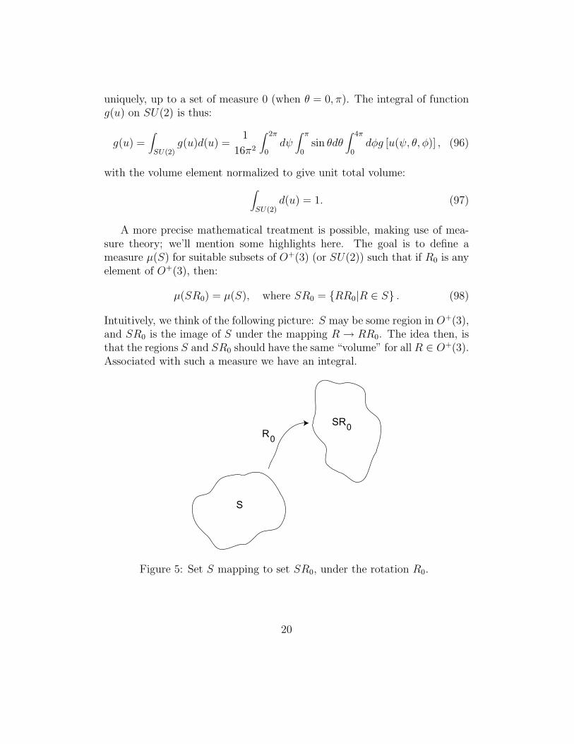
The argument for this form is as follows: We have a 1 : 1 correspondencebetween elements of O+(3) and orientations of a rigid body (such as a spherewith a dot at the north pole, centered at the origin; let I ∈ O+(3) correspondto the orientation with the north pole on the +e3 axis, and the meridian alongthe +e2 axis, say). We want to find a way to average over all positions of thesphere, with each orientation receiving the same weight. This correspondsto a uniform averaging over the sphere of the location of the north pole.

Now notice that if R(ψ, θ, φ) acts on the reference position, we obtainan orientation where the north pole has polar angles (θ, ψ). Thus, the (θ, ψ)dependence of d(R) must be dψ sin θdθ. For fixed (θ, ψ), the angle φ describesa rotation of the sphere about the north-south axis – the invariant integralmust correspond to a uniform averaging over this angle. Hence, we intuitivelyarrive at the above form for d(R). The constant K > 0 is arbitrary; we pickit for convenience. We shall choose K so that the integral over the entiregroup is one:

1 =∫

O+(3)d(R) =

1

8π2

∫ 2π

0dψ

∫ π

0sin θdθ

∫ 2π

0dφ. (92)

We can thus evaluate the integral of a (suitably behaved) function f(R) =f(ψ, θ, φ) over O+(3):

f(R) =∫

O+(3)f(R)d(R) =

1

8π2

∫ 2π

0dψ

∫ π

0sin θdθ

∫ 2π

0dφf(ψ, θ, φ). (93)

The overbar notation is intended to suggest an average.What about the invariant integral over SU(2)? Given the answer for

O+(3), we can obtain the result for SU(2) using the connection between thetwo groups. First, parameterize SU(2) by the Euler angles:

u(ψ, θ, φ) = exp(− i

2ψσ3

)exp

(− i

2θσ2

)exp

(− i

2φσ3

), (94)

with0 ≤ ψ < 2π; 0 ≤ θ ≤ π; 0 ≤ φ < 4π. (95)

Notice that the ranges are the same as for O+(3), except for the doubledrange required for φ. With these ranges, we obtain every element of SU(2),

19

uniquely, up to a set of measure 0 (when θ = 0, π). The integral of functiong(u) on SU(2) is thus:

g(u) =∫

SU(2)g(u)d(u) =

1

16π2

∫ 2π

0dψ

∫ π

0sin θdθ

∫ 4π

0dφg [u(ψ, θ, φ)] , (96)

with the volume element normalized to give unit total volume:

∫

SU(2)d(u) = 1. (97)

A more precise mathematical treatment is possible, making use of mea-sure theory; we’ll mention some highlights here. The goal is to define ameasure µ(S) for suitable subsets of O+(3) (or SU(2)) such that if R0 is anyelement of O+(3), then:

µ(SR0) = µ(S), where SR0 = RR0|R ∈ S . (98)

Intuitively, we think of the following picture: S may be some region in O+(3),and SR0 is the image of S under the mapping R → RR0. The idea then, isthat the regions S and SR0 should have the same “volume” for all R ∈ O+(3).Associated with such a measure we have an integral.

R

S

SR

00

Figure 5: Set S mapping to set SR0, under the rotation R0.

20

It may be shown2 that a measure with the desired property exists and isunique, up to a factor, for any finite-dimensional Lie group. Such a measureis called a Haar measure. The actual construction of such a measure mustdeal with coordinate system issues. For example, there may not be a goodglobal coordinate system on the group, forcing the consideration of localcoordinate systems.

Fortunately, we have already used our intuition to obtain the measure(volume element) for the Euler angle parameterization, and a rigorous treat-ment would show it to be correct. The volume element in other parameter-izations may be found from this one by suitable Jacobian calculations. Forexample, if we parameterize O+(3) by:

Re(θ) = eθθθ·JJJ , (99)

where θθθ ≡ θe, and |θθθ| ≤ π, then the volume element (normalized again tounit total volume of the group) is:

d(R) =1

4π2

1 − cos θ

θ2d3(θθθ), (100)

where d3(θθθ) is an ordinary volume element on R3. Thus, the group-averagedvalue of f(R) is:

∫

O+(3)f(R)d(R) =

1

4π2

∫

O+(3)

1 − cos θ

θ2d3(θθθ)f

(eθθθ·JJJ

)(101)

=1

4π2

∫

4πdΩe

∫ 2π

0(1 − cos θ)dθf

(eθθθ·JJJ

). (102)

Alternatively, we may substitute 1− cos θ = 2 sin2 θ2. For SU(2) we have the

corresponding result:

d(u) =1

4π2dΩe sin2 θ

2dθ, 0 ≤ θ ≤ 2π. (103)

We state without pro0f that the Haar measure is both left- and right-invariant. That is, µ(S) = µ(SR0) = µ(R0S) for all R0 ∈ O+(3) and for allmeasurable sets S ⊂ O+(3). This is to be hoped for on “physical” grounds.The invariant integral is known as the Haar integral, or its particular real-ization for the rotation group as the Hurwitz integral.

2This may be shown by construction, starting with a small neighborhood of the identity,and using the desired property to transfer the right volume element everywhere.

21

8 Unitary Representations of SU(2) (and O+(3))

A unitary representation of SU(2) is a mapping

u ∈ SU(2) → U(u) ∈ U(n) such that U(u′)U(u′′) = U(u′u′′), ∀u′, u′′ ∈ SU(2).(104)

That is, we “represent” the elements of SU(2) by unitary matrices (notnecessarily 2 × 2), such that the multiplication table is preserved, eitherhomomorphically or isomorphically. We are very interested in such mappings,because they permit the study of systems of arbitrary angular momenta,as well as providing the framework for adding angular momenta, and forstudying the angular symmetry properties of operators. We note that, forevery unitary representation R → T (R) of O+(3) there corresponds a unitaryrepresentation of SU(2): u→ U(u) = T [R(u)]. Thus, we focus our attentionon SU(2), without losing any generality.

For a physical theory, it seems reasonable to to demand some sort ofcontinuity structure. That is, whenever two rotations are near each other,the representations for them must also be close.

Def: A unitary representation U(u) is called weakly continuous if, for anytwo vectors φ, ψ, and any u:

limu′→u

〈φ| [U(u′) − U(u)]ψ〉 = 0. (105)

In this case, we write:

w-limu′→u

U(u′) = U(u), (106)

and refer to it as the “weak-limit”.

Def: A unitary representation U(u) is called strongly continuous if, forany vector φ and any u:

limu′→u

‖ [U(u′) − U(u)]φ‖ = 0. (107)

In this case, we write:

s-limu′→u

U(u′) = U(u), (108)

and refer to it as the “strong-limit”.

22

Strong continuity implies weak continuity, since:

|〈φ| [U(u′) − U(u)]ψ〉| ≤ ‖φ‖‖ [U(u′) − U(u)]ψ‖ (109)

We henceforth (i.e., until experiment contradicts us) adopt these notions ofcontinuity as physical requirements.

An important concept in representation theory is that of “(ir)reducibility”:

Def: A unitary representation U(u) is called irreducible if no subspace ofthe Hilbert space is mapped into itself by every U(u). Otherwise, therepresentation is said to be reducible.

Irreducible representations are discussed so frequently that the jargon “ir-rep” has emerged as a common substitute for the somewhat lengthy “irre-ducible representation”.

Lemma: A unitary representation U(u) is irreducible if and only if everybounded operator Q which commutes with every U(u) is a multiple ofthe identity.

Proof of this will be left as an exercise. Now for one of our key theorems:

Theorem: If u→ U(u) is a strongly continuous irreducible representation ofSU(2) on a Hilbert space H, then H has a finite number of dimensions.

Proof: The proof consists of showing that we can place a finite upper boundon the number of mutually orthogonal vectors in H: Let E be any one-dimensional projection operator, and φ, ψ be any two vectors in H.Consider the integral:

B(ψ, φ) =∫

SU(2)d(u)〈ψ|U(u)EU(u−1)φ〉. (110)

This integral exists, since the integrand is continuous and bounded,because U(u)EU(u−1) is a one-dimensional projection, hence of norm1.

Now

|B(ψ, φ)| =

∣∣∣∣∣

∫

SU(2)d(u)〈ψ|U(u)EU(u−1)φ〉

∣∣∣∣∣

≤∫

SU(2)d(u)|〈ψ|U(u)EU(u−1)φ〉| (111)

≤∫

SU(2)d(u)‖ψ‖‖φ‖‖U(u)EU(u−1)‖ (112)

≤ ‖ψ‖‖φ‖, (113)

23

where we have made use of the Schwarz inequality and of the fact∫SU(2) d(u) = 1.

B(ψ, φ) is linear in φ, anti-linear in ψ, and hence defines a boundedoperator B0 such that:

B(ψ, φ) = 〈ψ|B0φ〉. (114)

Let u0 ∈ SU(2). Then

〈ψ|U(u0)B0U(u−10 )φ〉 =

∫

SU(2)d(u)〈ψ|U(u0u)EU((u0u)

−1)φ〉(115)

=∫

SU(2)d(u)〈ψ|U(u)EU(u−1)φ〉 (116)

= 〈ψ|B0φ〉, (117)

where the second line follows from the invariance of the Haar integral.Since ψ and φ are arbitrary vectors, we thus have;

U(u0)B0 = B0U(u0), ∀u0 ∈ SU(2). (118)

Since B0 commutes with every element of an irreducible representation,it must be a multiple of the identity, B0 = pI.

∫

SU(2)d(u)U(u)EU(u−1) = pI. (119)

Now let φn|n = 1, 2, . . . , N be a set of N orthonormal vectors,〈φn|φm〉 = δnm, and take E = |φ1〉〈φ1|. Then,

〈φ1|∫

SU(2)d(u)U(u)EU(u−1)|φ1〉 = p〈φ1|I|φ1〉 = p, (120)

=∫

SU(2)d(u)〈φ1|U(u)|φ1〉〈φ1|U(u−1)|φ1〉

=∫

SU(2)d(u)|〈φ1|U(u)|φ1〉|2 > 0. (121)

Note that the integral cannot be zero, since the integrand is a contin-uous non-negative definite function of u, and is equal to one for u = I.

24

Thus, we have:

pN =N∑

n=1

〈φn|pIφn〉 (122)

=N∑

n=1

∫

SU(2)d(u)〈φn|U(u)EU(u−1)φn〉 (123)

=N∑

n=1

∫

SU(2)d(u)〈φn|U(u)|φ1〉〈φ1|U(u−1)φn〉 (124)

=N∑

n=1

∫

SU(2)d(u)〈U(u)φ1|φn〉〈φn|U(u)φ1〉 (125)

=∫

SU(2)d(u)〈U(u)φ1|

N∑

n=1

|φn〉〈φn|U(u)φ1〉 (126)

≤∫

SU(2)d(u)〈U(u)φ1|I|U(u)φ1〉 (127)

≤∫

SU(2)d(u)‖U(u)φ1‖2 = 1. (128)

(129)

That is, pN ≤ 1. But p > 0, so N < ∞, and hence H cannot containan arbitrarily large number of mutually orthogonal vectors. In otherwords, H is finite-dimensional.

Thus, we have the important result that if U(u) is irreducible, then theoperators U(u) are finite-dimensional unitary matrices. We will not have toworry about delicate issues that might arise if the situation were otherwise.3

Before actually building representations, we would like to know whetherit is “sufficient” to consider only unitary representations of SU(2).

Def: Two (finite dimensional) representations U and W of a group are calledequivalent if and only if they are similar, that is, if there exists afixed similarity transformation S which maps one representation ontothe other:

U(u) = SW (u)S−1, ∀u ∈ SU(2). (130)

Otherwise, the representations are said to be inequivalent.

3The theorem actually holds for any compact Lie group, since a Haar integral normal-ized to one exists.

25

Note that we can think of equivalence as just a basis transformation. Thedesired theorem is:

Theorem: Any finite-dimensional (continuous) representation u→W (u) ofSU(2) is equivalent to a (continuous) unitary representation u→ U(u)of SU(2).

Proof: We prove this theorem by constructing the required similarity trans-formation: Define matrix

P =∫

SU(2)d(u)W †(u)W (u). (131)

This matrix is positive definite and Hermitian, since the integrand is.Thus P has a unique positive-definite Hermitian square root S:

P = P † > 0 =⇒√P = S = S† > 0. (132)

Now, let u0, u ∈ SU(2). We have,

W †(u0)W†(u)W (u) =

[W †(uu0)W (uu0)

]W (u−1

0 ). (133)

From the invariance of the Haar integral, we find:

W †(u0)P =∫

SU(2)d(u)

[W †(uu0)W (uu0)

]W (u−1

0 ) (134)

= PW (u−10 ), ∀u0 ∈ SU(2). (135)

Now define, for all u ∈ SU(2),

U(u) = SW (u)S−1. (136)

The mapping u→ U(u) defines a continuous representation of SU(2),and furthermore:

U †(u)U(u) =[SW (u)S−1

]† [SW (u)S−1

]

=(S−1

)†W †(u)S†SW (u)S−1

=(S−1

)†PW †(u−1)W (u)S−1

=(S−1

)†PS−1

=(S−1

)†S†SS−1

= I. (137)

That is, U(u) is a unitary representation, equivalent to W (u).

26

We have laid the fundamental groundwork: It is sufficient to determine allunitary finite-dimensional irreducible representations of SU(2).

This brings us to some important “tool theorems” for working in grouprepresentaion theory.

Theorem: Let u → D′(u) and u → D′′(u) be two inequivalent irreduciblerepresentations of SU(2). Then the matrix elements ofD′(u) andD′′(u)satisfy: ∫

SU(2)d(u)D′

mn(u)D′′rs(u) = 0. (138)

Proof: Note that the theorem can be thought of as a sort of orthogonalityproperty between matrix elements of inequivalent representations. LetV ′ be the N ′-dimensional carrier space of the representation D′(u), andlet V ′′ be the N ′′-dimensional carrier space of the representation D′′(u).Let A be any N ′ ×N ′′ matrix. Define another N ′ ×N ′′ matrix, A0 by:

A0 ≡∫

SU(2)d(u)D′(u−1)AD′′(u). (139)

Consider (in the sceond line, we use the invariance of the Haar integralunder the substitution u→ uu0):

D′(u0)A0 =∫

SU(2)d(u)D′(u0u

−1)AD′′(u)

=∫

SU(2)d(u)D′(u−1)AD′′(uu0)

=∫

SU(2)d(u)D′(u−1)AD′′(u)D′′(u0)

= A0D′′(u0), ∀u0 ∈ SU(2). (140)

Now define N ′ ×N ′ matrix B′ and N ′′ ×N ′′ matrix B′′ by:

B′ ≡ A0A†0, B′′ ≡ A†

0A0. (141)

Then we have:

D′(u)B′ = D′(u)A0A†0

= A0D′′(u)A†

0

= A0A†0D

′(u)

= B′D′(u), ∀u ∈ SU(2). (142)

27

Similarly,D′′(u)B′′ = B′′D′′(u), ∀u ∈ SU(2). (143)

Thus, B′, an operator on V ′, commutes with all elements of irreduciblerepresentation D′, and is therefore a multiple of the identity operatoron V ′: B′ = b′I ′. Likewise, B′′ = b′′I ′′ on V ′′.

If A0 6= 0, this can be possible only if N ′ = N ′′, and A0 is non-singular. But if A0 is non-singular, then D′ and D′′ are equivalent,since D′(u)A0 = A0D

′′, ∀u ∈ SU(2). But this contradicts the as-sumption in the theorem, hence A0 = 0. To complete the proof, selectAnr = 1 for any desired n, r and set all of the other elements equal tozero.

Next, we quote the corresponding “orthonormality” theorem among ele-ments of the same irreducible representation:

Theorem: Let u → D(u) be a (continuous) irreducible representation ofSU(2) on a carrier space of dimension d. Then

∫

SU(2)d(u)Dmn(u

−1)Drs(u) = δmsδnr/d. (144)

Proof: The proof of this theorem is similar to the preceding theorem. LetA be an arbitrary d× d matrix, and define

A0 ≡∫

SU(2)d(u)D(u−1)AD(u). (145)

As before, we may show that

D(u)A0 = A0D(u), (146)

and hence A0 = aI is a multiple of the identity. We take the trace tofind the multiple:

a =1

dTr

[∫

SU(2)d(u)D(u−1)AD(u)

](147)

=1

d

∫

SU(2)d(u)Tr

[D(u−1)AD(u)

](148)

=1

dTrA. (149)

28

This yields the result

∫

SU(2)d(u)D(u−1)AD(u) =

Tr(A)

dI. (150)

Again, select A with any desired element equal to one, and all otherelements equal to 0, to finish the proof.

We consider now the set of all irreducible representations of SU(2). Moreprecisely, we do not distinguish between equivalent representations, so this setis the union of all equivalence classes of irreducible representations. Use thesymbol j to label an equivalence class, i.e., j is an index, taking on values inan index set in 1:1 correspondence with the set of all equivalence classes. Wedenote D(u) = Dj(u) to indicate that a particular irreducible representationu → D(u) belongs to equivalence class “j”. Two representations Dj(u) andDj′(u) are inequivalent if j 6= j ′. Let dj be the dimension associated withequivalence class j. With this new notation, we may restate our above twotheorems in the form:

∫

SU(2)d(u)Dj

mn(u−1)Dj′

rs =1

dδjj′δmsδnr. (151)

This is an important theorem in representation theory, and is sometimesreferred to as the “General Orthogonality Relation”.

For much of what we need, we can deal with simpler objects than the fullrepresentation matrices. In particular, the traces are very useful invariantsunder similarity transformations. So, we define:

Def: The character χ(u) of a finite-dimensional representation u → D(u)of SU(2) is the function on SU(2):

χ(u) = Tr [D(u)] . (152)

We immediately remark that the characters of two equivalent representationsare identical, since

Tr[SD(u)S−1

]= Tr [D(u)] . (153)

In fact, we shall see that the representation is completely determined by thecharacters, up to similarity transformations.

Let χj(u) denote the character of irreducible representation Dj(u). Theindex j uniquely determines χj(u). We may summarize some importantproperties of characters in a theorem:

29

Theorem: 1. For any finite-dimensional representation u→ D(u) of SU(2):

χ(u0uu−10 ) = χ(u), ∀u, u0 ∈ SU(2). (154)

2.χ(u) = χ∗(u) = χ(u−1) = χ(u∗), ∀u ∈ SU(2). (155)

3. For the irreducible representations u→ Dj(u) of SU(2):∫

SU(2)d(u)χj(u0u

−1)Dj′(u) =1

djδjj′D

j(u0) (156)

∫

SU(2)d(u)χj(u0u

−1)χj′(u) =1

djδjj′χj(u0) (157)

∫

SU(2)d(u)χj(u

−1)χj′(u) =∫

SU(2)d(u)χ∗

j(u)χj′(u) = δjj′. (158)

Proof: (Selected portions)

1.

χ(u0uu−10 ) = Tr

[D(u0uu

−10 )]

= Tr[D(u0)D(u)D(u−1

0 )]

= χ(u). (159)

2.

χ(u−1) = Tr[D(u−1)

]= Tr

[D(u)−1

]

= Tr[(SU(u)S−1)−1

], where U is a unitary representation,

= Tr[S−1U †(u)S

]

= Tr[U †(u)

]

= χ∗(u). (160)

The property χ(u) = χ(u∗) holds for SU(2), but not more gener-ally [e.g., it doesn’t hold for SU(3)]. It holds for SU(2) becausethe replacement u → u∗ gives an equivalent representation forSU(2). Let us demonstrate this. Consider the parameterization:

u = ue(θ) = cosθ

2I − i sin

θ

2e · σσσ. (161)

30

Now form the complex conjugate, and make the following similar-ity transformation:

σ2u∗σ−1

2 = σ2

[cos

θ

2I + i sin

θ

2e · σσσ∗σ−1

2

]

= cosθ

2I + i sin

θ

2[e1σ2σ1σ2 − e2σ2σ2σ2 + e3σ2σ3σ2]

= cosθ

2I − i sin

θ

2e · σσσ

= u. (162)

We thus see that u and u∗ are equivalent representations forSU(2). Now, for representation D (noting that iσ2 ∈ SU(2)):

D(u) = D(iσ2)D(u∗)D−1(iσ2), (163)

and hence, χ(u) = χ(u∗).

3. We start with the general orthogonality relation, and use

χj(u0u−1) =

∑

m,n

Djnm(u0)D

jmn(u

−1), (164)

to obtain∫

SU(2)d(u)χj(u0u

−1)Dj′

rs(u) =∫

SU(2)d(u)

∑

m,n

Djnm(u0)D

jmn(u

−1)Dj′

rs(u)

=∑

m,n

Djnm(u0)

1

djδjj′δnrδms

=1

djδjj′D

jrs(u0). (165)

Now take the trace of both sides of this, as a matrix equation:

∫

SU(2)d(u)χj(u0u

−1)χj′(u) =1

djδjj′χj(u0). (166)

Let u0 = I. The character of the identity is just dj, hence weobtain our last two relations.

31

9 Reduction of Representations

Theorem: Every continuous finite dimensional representation u→ D(u) ofSU(2) is completely reducible, i.e., it is the direct sum:

D(u) =∑

r

⊕Dr(u) (167)

of a finite number of irreps Dr(u). The multiplicities mj (the numberof irreps Dr which belong to the equivalence class of irreps characterizedby index j) are unique, and they are given by:

mj =∫

SU(2)d(u)χj(u

−1)χ(u), (168)

where χ(u) = Tr [D(u)]. Two continuous finite dimensional represen-tations D′(u) and D′′(u) are equivalent if and only if their charactersχ′(u) and χ′′(u) are identical as functions on SU(2).

Proof: It is sufficient to consider the case where D(u) is unitary and re-ducible. In this case, there exists a proper subspace of the carrierspace of D(u), with projection E ′, which is mapped into itself by D(u):

E ′D(u)E ′ = D(u)E ′. (169)

Take the hermitian conjugate, and relabel u→ u−1:

[E ′D(u−1)E ′

]†=

[D(u−1)E ′

]†(170)

E ′D†(u−1)E ′ = E ′D†(u−1) (171)

E ′D(u)E ′ = E ′D(u). (172)

Hence, E ′D(u) = D(u)E ′, for all elements u in SU(2).

Now, let E ′′ = I − E ′ be the projection onto the subspace orthogonalto E ′. Then:

D(u) = (E ′ + E ′′)D(u)(E ′ + E ′′) (173)

= E ′D(u)E ′ + E ′′D(u)E ′′ (174)

(since, e.g., E ′D(u)E ′′ = D(u)E ′E ′′ = D(u)E ′(I − E ′) = 0). Thisformula describes a reduction of D(u). If D(u) restricted to subspace

32

E ′ (or E ′′) is reducible, we repeat the process until we have only ir-reps remaining. The finite dimensionality of the carrier space of D(u)implies that there are a finite number of steps to this procedure.

Thus, we obtain a set of projections Er such that

I =∑

r

Er (175)

ErEs = δrsEr (176)

D(u) =∑

r

ErD(u)Er, (177)

where D(u) restricted to any of subspaces Er is irreducible:

D(u) =∑

r

⊕Dr(u). (178)

The multiplicity follows from

∫

SU(2)d(u)χj(u

−1)χj′(u) = δjj′. (179)

Thus,

∫

SU(2)d(u)χj(u

−1)χ(u) =∫

SU(2)χj(u

−1)Tr

[∑

r

⊕Dr(u)

](180)

= the number of terms in the sum

with Dr = Dj (181)

= mj. (182)

Finally, suppose D′(u) and D′′ are equivalent. We have already shownthat the characters must be identical. Suppose, on the other hand, thatD′(u) and D′′ are inequivalent. In this case, the characters cannot beidentical, or this would violate our other relations above, as the readeris invited to demonstrate.

10 The Clebsch-Gordan Series

We are ready to embark on solving the problem of the addition of angularmomenta. Let D′(u) be a representation of SU(2) on carrier space V ′, and

33

let D′′(u) be a representation of SU(2) on carrier space V ′′, and assume V ′

and V ′′ are finite dimensional. Let V = V ′ ⊗ V ′′ denote the tensor productof V ′ and V ′′.

The representations D′ and D′′ induce a representation on V in a naturalway. Define the representation D(u) on V in terms of its action on any φ ∈ Vof the form φ = φ′ ⊗ φ′′ as follows:

D(u)(φ′ ⊗ φ′′) = [D′(u)φ′] ⊗ [D′′(u)φ′′] . (183)

Denote this representation as D(u) = D′(u) ⊗D′′(u) and call it the tensorproduct of D′ and D′′. The matrix D(u) is the Kronecker product of D′(u)and D′′(u). For the characters, we clearly have

χ(u) = χ′(u)χ′′(u). (184)

We can extend this tensor product definition to the product of any finitenumber of representations.

The tensor product of two irreps, Dj′(u) and Dj′′(u), is in general notirreducible. We know however, that it is completely reducible, hence a directsum of irreps:

Dj′(u) ⊗Dj′′(u) =∑

j

⊕Cj′j′′jDj(u). (185)

This is called a “Clebsch-Gordan series”. The Cj′j′′j coefficients are some-times referred to as Clebsch-Gordan coefficients, although we tend to use thatname for a different set of coefficients. These coefficients must, of course, benon-negative integers. We have the corresponding identity:

χj′(u)χj′′(u) =∑

j

Cj′j′′jχj(u). (186)

We now come to the important theorems on combining angular momentain quantum mechanics:

Theorem:

1. There exists only a countably infinite number of inequivalent ir-reps of SU(2). For every positive integer (2j+1), j = 0, 1

2, 1, 3

2, . . .,

there exists precisely one irrep Dj(u) (up to similarity transforma-tions) of dimension (2j + 1). As 2j runs through all non-negativeintegers, the representations Dj(u) exhaust the set of all equiva-lence classes.

34

2. The character of irrep Dj(u) is:

χj [ueee(θ)] =sin 2j+1

2θ

sin 12θ, (187)

andχj(I) = dj = 2j + 1. (188)

3. The representation Dj(u) occurs precisely once in the reductionof the 2j-fold tensor product (⊗u)2j, and we have:

∫

SU(2)d(u)χj(u) [Tr(u)]2j = 1. (189)

Proof: We take from∫SU(2) d(u)χ

∗j(u)χj′(u) = δjj′ the suggestion that the

characters of the irreps are a complete set of orthonormal functionson a Hilbert space of class-functions of SU(2) (A class-function is afunction which takes the same value for every element in a conjugateclass).

Consider the following function on SU(2):

ω(u) ≡ 1 − 1

8Tr[(u− I)†(u− I)

]=

1

2

[1 +

1

2Tr(u)

], (190)

which satisfies the conditions 1 > ω(u) ≥ 0 for u 6= I, and u(I) = 1(e.g., noting that ueee(θ) = cos θ

2I + a traceless piece). Hence, we have

the lemma: If f(u) is a continuous function on SU(2), then

limn→∞

∫SU(2) d(u)f(u) [ω(u)]n∫SU(2) d(u) [ω(u)]n

= f(I). (191)

The intuition behind this lemma is that, as n → ∞, [ω(u)]n becomesincreasingly peaked about u = I.

Thus, if Dj(u) is any irrep of SU(2), then there exists an integer n suchthat: ∫

SU(2)d(u)χj(u

−1) [Tr(u)]n 6= 0. (192)

Therefore, the irrep Dj(u) occurs in the reduction of the tensor product(⊗u)n.

35

Next, we apply the Gram-Schmidt process to the infinite sequence[Tr(u)]n |n = 0, 1, 2, . . . of linearly independent class functions on SU(2)to obtain the orthonormal sequence Bn(u)|n = 0, 1, 2, . . . of classfunctions:∫

SU(2)d(u)B∗

n(u)Bm(u) =1

π

∫ 2π

0dθ sin2 θ

2B∗n [ue3(θ)]Bm [ue3(θ)] = δnm,

(193)where we have used the measure d(u) = 1

4π2dΩeee sin2 θ2dθ and the fact

that, since Bn is a class function, it has the same value for a rotationby angle θ about any axis.

Now, writeβn(θ) = Bn [ue3(θ)] = Bn [ueee(θ)] . (194)

Noting that

[Tr(u)]n =

(2 cos

θ

2

)n=

n∑

m=0

(n

m

)eiθ(

n2−m), (195)

we may obtain the result

βn(θ) =sin [(n+ 1)θ/2]

sin θ/2= Bn [ueee(θ)] = B∗

n [ueee(θ)] , (196)

by adopting suitable phase conventions for the B’s. Furthermore,∫

SU(2)d(u)B∗

n(u) [Tr(u)]m =

0 if n > m,1 if n = m.

(197)

We need to prove now that the functions Bn(u) are characters of theirreps. We shall prove this by induction on n. First, B0(u) = 1; B0(u) isthe character of the trivial one-dimensional identity representation:D(u) = 1. Assume now that for some integer n0 ≥ 0 the functionsBn(u) for n = 0, 1, . . . , n0 are all characters of irreps. Consider thereduction of the representation (⊗u)n0+1:

[Tr(u)]n0+1 =n0∑

n=0

Nn0,nBn(u) +∑

j∈Jn0

cn0,jχj(u), (198)

where Nn0,n and cn0,j are integers ≥ 0, and the cn0,j sum is over irrepsDj such that the characters are not in the set Bn(u)|n = 0, 1, . . . , n0(j runs over a finite subset of the Jn0 index set).

36

With the above fact that:∫

SU(2)d(u)B∗

n(u) [Tr(u)]n0+1 =

0 if n > n0 + 1,1 if n = n0 + 1,

(199)

we have,Bn0+1(u) =

∑

j∈Jn0

cn0,jχj(u). (200)

Squaring both sides, and averaging over SU(2) yields

1 =∑

j∈Jn0

(cn0,j)2. (201)

But the cn0,j are integers, so there is only one term, with cn0,j = 1.Thus, Bn0+1(u) is a character of an irrep, and we see that there are acountably infinite number of (inequivalent) irreducible representations.

Let us obtain the dimensionality of the irreducible representation. TheBn(u), n = 0, 1, 2, . . . correspond to characters of irreps. We’ll labelthese irredusible representations Dj(u) according to the 1 : 1 mapping2j = n. Then

dj = χj(I) = B2j(I) = β2j(0) (202)

= limθ→0

sin [(2j + 1)θ/2]

sin θ/2(203)

= 2j + 1. (204)

Next, we consider the reduction of the tensor product of two irreduciblerepresentations of SU(2). This gives our “rule for combining angular momen-tum”. That is, it tells us what angular momenta may be present in a systemcomposed of two components with angular momenta. For example, it maybe applied to the combination of a spin and an orbital angular momentum.

Theorem: Let j1 and j2 index two irreps of SU(2). Then the Clebsch-Gordan series for the tensor product of these representations is:

Dj1(u) ⊗Dj2(u) =j1+j2∑

j=|j1−j2|⊕Dj(u). (205)

37

Equivalently,

χj1(u)χj2(u) =j1+j2∑

j=|j1−j2|χj(u) =

∑

j

Cj1j2jχj(u), (206)

where

Cj1j2j =∫

SU(2)d(u)χj1(u)χj2(u)χj(u) (207)

=

1 iff j1 + j2 + j is an integer, and a triangle canbe formed with sides j1, j2, j,

0 otherwise.

(208)

The proof of this theorem is straightforward, by considering

Cj1j2j =1

π

∫ 2π

0dθ sin

[(j1 +

1

2)θ]sin

[(j2 +

1

2)θ] j∑

m=−je−imθ, (209)

etc., as the reader is encouraged to carry out.We have found all the irreps of SU(2). Which are also irreps of O+(3)?

This is the subject of the next theorem:

Theorem: If 2j is an odd integer, then Dj(u) is a faithful representationof SU(2), and hence is not a representation of O+(3). If 2j > 0 is aneven integer (and hence j > 0 is an integer), then Reee(θ) → Dj[ueee(θ)]is a faithful representation of O+(3). Except for the trivial identityrepresentation, all irreps of O+(3) are of this form.

The proof of this theorem is left to the reader.We will not concern ourselves especially much with issues of constructing

a proper Hilbert space, such as completeness, here. Instead, we’ll concentrateon making the connection between SU(2) representation theory and angularmomentum in quantum mechanics a bit more concrete. We thus introducethe quantum mechanical angular momentum operators.

Theorem: Let u→ U(u) be a (strongly-)continuous unitary representationof SU(2) on Hilbert space H. Then there exists a set of 3 self-adjointoperators Jk, k = 1, 2, 3 such that

U [ueee(θ)] = exp(−iθeee · JJJ). (210)

38

To keep things simple, we’ll consider now U(u) = D(u), where D(u) isa finite-dimensional representation – the appropriate extension to thegeneral case may be demonstrated, but takes some care, and we’ll omitit here.

1. The function D[ueee(θ)] is (for eee fixed), an infinitely differentiablefunction of θ. Define the matrices J(eee) by:

J(eee) ≡ i

∂

∂θD [ueee(θ)]

θ=0

. (211)

Also, let J1 = J(eee1), J2 = J(eee2), J3 = J(eee3). Then

J(eee) = eee · JJJ =3∑

k=1

(eee · eeek)Jk. (212)

For any unit vector eee and any θ, we have

D [ueee(θ)] = exp(−iθeee · JJJ). (213)

The matrices Jk satisfy:

[Jk, J`] = iεk`mJm. (214)

The matrices −iJk, k = 1, 2, 3 form a basis for a representation ofthe Lie algebra of O+(3) under the correspondence:

Jk → −iJk, k = 1, 2, 3. (215)

The matrices Jk are hermitian if and only if D(u) is unitary.

2. The matrices Jk, k = 1, 2, 3 form an irreducible set if and only ifthe representation D(u) is irreducible. If D(u) = Dj(u) is irre-ducible, then for any eee, the eigenvalues of eee · JJJ are the numbersm = −j,−j + 1, . . . , j − 1, j, and each eigenvalue has multiplicityone. Furthermore:

JJJ2 = J21 + J2

2 + J23 = j(j + 1). (216)

3. For any representation D(u) we have

D(u)JJJ2D(u−1) = JJJ2; [Jk,JJJ2] = 0, k = 1, 2, 3. (217)

39

Proof: (Partial) Consider first the case where D(u) = Dj(u) is an irrep. LetMj = m|m = −j, . . . , j, let eee be a fixed unit vector, and define theoperators Fm(eee) (with m ∈Mj) by:

Fm(eee) ≡ 1

4π

∫ 4π

0dθeimθDj[ueee(θ)]. (218)

Multiply this defining equation by Dj[ueee(θ′)]:

Dj[ueee(θ′)]Fm(eee) =

1

4π

∫ 4π

0dθeimθDj[ueee(θ + θ′)] (219)

=1

4π

∫ 4π

0dθeim(θ−θ′)Dj[ueee(θ)] (220)

= e(−imθ′)Fm(eee). (221)

Thus, either Fm(eee) = 0, or e(−imθ′) is an eigenvalue of Dj[ueee(θ

′)]. But

χj[ueee(θ)] =j∑

n=−je−inθ, (222)

and hence,

Tr[Fm(eee)] =

1 if m ∈Mj,0 otherwise.

(223)

Therefore, Fm(eee) 6= 0.

We see that the Fm(eee) form a set of 2j+1 independent one-dimensionalprojection operators, and we can represent the Dj(u) by:

Dj[ueee(θ)] =j∑

m=−je−imθFm(eee). (224)

From this, we obtain:

J(eee) ≡ i

∂

∂θDj [ueee(θ)]

θ=0

=j∑

m=−jmFm(eee), (225)

andDj[ueee(θ)] = exp [−iθJ(eee)] , (226)

which is an entire function of θ for fixed eee.

40

Since every finite-dimensional continuous representation D(u) is a di-rect sum of a finite number of irreps, this result holds for any suchrepresentation:

D[ueee(θ)] = exp [−iθJ(eee)] . (227)

Let www be a unit vector with components wk, k = 1, 2, 3. Consider“small” rotations about www:

uwww(θ) = ueee1(θw1)ueee2(θw2)ueee3(θw3)ueee(θ,www)[α(θ,www)], (228)

where α(θ,www) = O(θ2) for small θ. Thus,

exp [−iθJ(www)] = e−iθw1J1e−iθw2J2e−iθw3J3e−iαJ(eee). (229)

Expanding the exponentials and equating coefficients of terms linear inθ yields the result:

J(www) = w1J1 + w2J2 + w3J3 = www · JJJ. (230)

To obtain the commutation relations, consider

ueee1(θ)ueee2(θ′)u−1

eee1(θ) (231)

=

(cos

θ

2I − i sin

θ

2σ1

)(cos

θ′

2I − i sin

θ′

2σ2

)(232)

(cos

θ

2I + i sin

θ

2σ1

)(233)

= cosθ′

2I − i sin

θ′

2(cos θσ2 + sin θσ3) (234)

= ueee2 cos θ+eee3 sin θ(θ′). (235)

Thus,

exp(−iθJ1) exp(−iθ′J2) exp(iθJ1) = exp [−iθ′(J2 cos θ + J3 sin θ)] .(236)

Expanding the exponentials, we have:

∞∑

n=0

∞∑

`=0

∞∑

m=0

θn+mθ′`J

n1 J

`2J

m1

n!`!m!(−i)n+`im =

∞∑

r=0

(−i)rθ′r(J2 cos θ+J3 sin θ)r1

r!.

(237)

41

We equate coefficients of the same powers of θ, θ′. In particular, theterms of order θθ′ yield the result:

[J1, J2] = iJ3. (238)

We thus also have, for example:

[J1,JJJ2] = [J1, J

21 + J2

2 + J23 ] (239)

= J1J2J2 − J2J2J1 + J1J3J3 − J3J3J1 (240)

= (iJ3 + J2J1)J2 − J2(−iJ3 + J1J2) + (241)

(−iJ2 + J3J1)J3 − J3(iJ2 + J1J3) (242)

= 0. (243)

As a consequence, we also have:

D(u)JJJ2D(u−1) = e−iθeee·JJJJJJ2eiθeee·JJJ = JJJ2. (244)

In particular, this is true for an irrep:

Dj(u)JJJ2Dj(u−1) = JJJ2. (245)

Therefore JJJ2 is a multiple of the identity (often referred to as a “casimiroperator”).

Let us determine the multiple. Take the trace:

Tr(JJJ2) = 3Tr(J23 ) (246)

= 3Tr

∂

∂θDj [ueee3(θ)]

2

θ=0

(247)

= −3Tr

lim∆→0∆′→0

1

∆∆′

[Dj (ueee3(θ + ∆)) −Dj (ueee3(θ))

](248)

[Dj (ueee3

(θ + ∆′)) −Dj (ueee3(θ))

]

θ=0

(249)

= −3Tr

lim∆→0∆′→0

1

∆∆′

[Dj (ueee3(∆ + ∆′)) (250)

−Dj (ueee3(∆′)) −Dj (ueee3(∆)) +Dj (ueee3(0))

](251)

42

= −3Tr

[∂2

∂θ2Dj [ueee3(θ)]

]

θ=0

(252)

= −3

∂2

∂θ2χj [ueee3(θ)]

θ=0

. (253)

There are different ways to evaluate this. We could insert

χj [ueee3(θ)] =sin(j + 1

2)θ

sin 12θ

, (254)

or we could use

χj [ueee3(θ)] =

j∑

m=−jeimθ. (255)

In either case, we find:

Tr(JJJ2) = j(j + 1)(2j + 1). (256)

Since dj = 2j + 1, this gives the familiar result:

JJJ2 = j(j + 1)I. (257)

Finally, we’ll compute the eigenvalues of eee ·JJJ = J(eee) =∑jm=−jmFm(eee).

We showed earlier that the Fm(eee) are one-dimensional projection oper-ators, and it thus may readily be demonstrated that

J(eee)Fm(eee) = mFm(eee). (258)

Hence, the desired eigenvalues are m = −j,−j + 1, . . . , j − 1, j.

11 Standard Conventions

Let’s briefly summarize where we are. We’ll pick some “standard” conven-tions towards building explicit representations for rotations in quantum me-chanics.

• The rotation group in quantum mechanics is postulated to be SU(2),with elements

u = ueee(θ) = e−i2θeee·σσσ, (259)

describing a rotation by angle θ about vector eee, in the clockwise senseas viewed along eee.

43

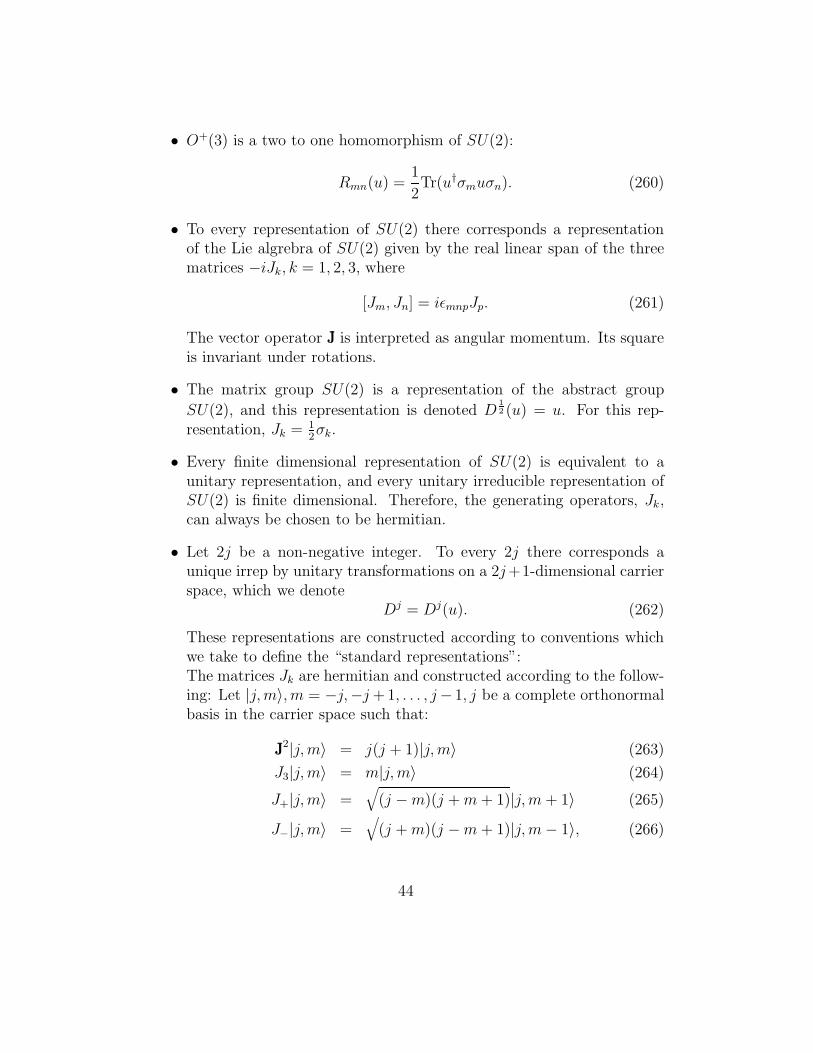
• O+(3) is a two to one homomorphism of SU(2):

Rmn(u) =1

2Tr(u†σmuσn). (260)

• To every representation of SU(2) there corresponds a representationof the Lie algrebra of SU(2) given by the real linear span of the threematrices −iJk, k = 1, 2, 3, where

[Jm, Jn] = iεmnpJp. (261)

The vector operator JJJ is interpreted as angular momentum. Its squareis invariant under rotations.

• The matrix group SU(2) is a representation of the abstract group

SU(2), and this representation is denoted D12 (u) = u. For this rep-

resentation, Jk = 12σk.

• Every finite dimensional representation of SU(2) is equivalent to aunitary representation, and every unitary irreducible representation ofSU(2) is finite dimensional. Therefore, the generating operators, Jk,can always be chosen to be hermitian.

• Let 2j be a non-negative integer. To every 2j there corresponds aunique irrep by unitary transformations on a 2j+1-dimensional carrierspace, which we denote

Dj = Dj(u). (262)

These representations are constructed according to conventions whichwe take to define the “standard representations”:The matrices Jk are hermitian and constructed according to the follow-ing: Let |j,m〉, m = −j,−j +1, . . . , j− 1, j be a complete orthonormalbasis in the carrier space such that:

JJJ2|j,m〉 = j(j + 1)|j,m〉 (263)

J3|j,m〉 = m|j,m〉 (264)

J+|j,m〉 =√

(j −m)(j +m + 1)|j,m + 1〉 (265)

J−|j,m〉 =√

(j +m)(j −m + 1)|j,m− 1〉, (266)

44

whereJ± ≡ J1 ± iJ2. (267)

According to convention, matrices J1 and J3 are real, and matrix J2 ispure imaginary. The matrix

Dj [ueee(θ)] = exp(−iθeee · JJJ), (268)

describes a rotation by θ about unit vector eee.

• If j = 12-integer, then Dj(u) are faithful representations of SU(2). If j

is an integer, then Dj(u) are representations of O+(3) (and are faithfulif j > 0). Also, if j is an integer, then the representation Dj(u) issimilar to a representation by real matrices:

Rmn(u) =3

j(j + 1)(2j + 1)Tr[Dj†(u)JmD

j(u)Jn]. (269)

• In the standard basis, the matrix elements of Dj(u) are denoted:

Djm1m2

(u) = 〈j,m1|Dj(u)|j,m2〉, (270)

and thus,

Dj(u)|j,m〉 =j∑

m′=−jDjm′m(u)|j,m′〉. (271)

Let |φ〉 be an element in the carrier space of Dj, and let |φ′〉 = Dj(u)|φ〉be the result of applying rotation Dj(u) to |φ〉. We may expand thesevectors in the basis:

|φ〉 =∑

m

φm|j,m〉 (272)

|φ′〉 =∑

m

φ′m|j,m〉. (273)

Thenφ′m =

∑

m′Djmm′(u)φm′. (274)

• Since matrices u and Dj(u) are unitary,

Djm1m2

(u−1) = Djm1m2

(u†) = D∗jm2m1

(u). (275)

45

• The representation Dj is the symmetrized (2j)-fold tensor product of

the representation D12 = SU(2) with itself. For the standard repre-

sentation, this is expressed by an explicit formula for matrix elementsDjm1m2

(u) as polynomials of degree 2j in the matrix elements of SU(2):Define the quantities Dj

m1m2(u) for m1, m2 = −j, . . . , j by:

〈λ∗|u|η〉2j = (λ1u11η1 + λ1u12η2 + λ2u21η1 + λ2u22η2)2j (276)

= (2j)!∑

m1,m2

(277)

λj+m11 λj−m1

2 ηj+m21 ηj−m2

2√(j +m1)!(j −m1)!(j +m2)!(j −m2)!

Djm1m2

(u).

We defer to later the demonstration that the matrix elements Djm1m2

(u)so defined are identical with the earlier definition for the standard rep-resentation. A consequence of this formula (which the reader is encour-aged to demonstrate) is that, in the standard representation,

Dj(u∗) = D∗j(u) (278)

Dj(uT ) = DjT (u). (279)

Also, noting that u∗ = σ2uσ2, we obtain

D∗j(u) = exp(−iπJ2)Dj(u) exp(iπJ2), (280)

making explicit our earlier statement that the congugate representationwas equivalent in SU(2) [We remark that this property does not holdfor SU(n), if n > 2].

• We can also describe the standard representation in terms of an ac-tion of the rotation group on homogeneous polynomials of degree 2jof complex variables x and y. We define, for each j = 0, 1

2, 1, . . ., and

m = −j, . . . , j the polynomial:

Pjm(x, y) ≡ xj+myj−m√(j +m)!(j −m)!

; P00 ≡ 1. (281)

We also define Pjm ≡ 0 if m /∈ −j, . . . , j. In addition, define thedifferential operators Jk, k = 1, 2, 3, J+, J−:

J3 =1

2(x∂x − y∂y) (282)

46

J1 =1

2(x∂y + y∂x) =

1

2(J+ + J−) (283)

J2 =i

2(y∂x − x∂y) =

i

2(J− − J+) (284)

J+ = x∂y = J1 + iJ2 (285)

J− = y∂x = J1 − iJ2 (286)

These definitions give

JJJ2 =1

4

[(x∂x − y∂y)

2 + 2(x∂x + y∂y)]. (287)

We let these operators act on our polynomials:

J3Pjm(x, y) =[1

2(x∂x − y∂y)

]xj+myj−m√

(j +m)!(j −m)!(288)

=1

2[j +m− (j −m)]Pjm(x, y) (289)

= mPjm(x, y). (290)

Similarly,

J+Pjm(x, y) = (x∂y)xj+myj−m√

(j +m)!(j −m)!(291)

= (j −m)xj+m+1yj−m−1

√(j +m)!(j −m)!

(292)

= (j −m)

√√√√(j +m+ 1)!(j −m− 1)!

(j +m)!(j −m)!Pj,m+1(x, y)

=√

(j −m)(j +m+ 1)Pj,m+1(x, y). (293)

Likewise,

J−Pjm(x, y) =√

(j +m)(j −m + 1)Pj,m−1(x, y), (294)

andJJJ2Pjm(x, y) = j(j + 1)Pjm(x, y). (295)

We see that the actions of these differential operators on the monomials,Pjm, are according to the standard representation of the Lie algebra of

47

the rotation group (that is, we compare with the actions of the standardrepresentation for JJJ on orthonormal basis |j,m〉).Thus, regarding Pjm(x, y) as our basis, a rotation corresponds to:

Dj(u)Pjm(x, y) =∑

m′Djm′m(u)Pjm′(x, y). (296)

Now,

D12 (u)P 1

2m(x, y) =

∑

m′D

12m′m(u)P 1

2m′(x, y) (297)

=∑

m′um′m(u)P 1

2m′(x, y). (298)

Or,uP 1

2m(x, y) = u 1

2mP 1

212(x, y) + u− 1

2mP 1

2− 1

2(x, y). (299)

With P 12

12(x, y) = x, and P 1

2− 1

2(x, y) = y, we thus have (using normal

matrix indices now on u)

uP 12

12(x, y) = u11x+ u21y, (300)

uP 12− 1

2(x, y) = u12x+ u22y. (301)

Hence,

Dj(u)Pjm(x, y) = Pjm(u11x + u21y, u12x + u22y) (302)

=∑

m′Djm′m(u)Pjm′(x, y). (303)

Any homogeneous polynomial of degree 2j in (x, y) can be written as aunique linear combination of the monomials Pjm(x, y). Therefore, theset of all such polynomials forms a vector space of dimension 2j + 1,and carries the standard representation Dj of the rotation group if theaction of the group elements on the basis vectors Pjm is as above. Notethat

Pjm(∂x, ∂y)Pjm′(x, y) =∂j+mx ∂j−my xj+m

′yj−m

′

√(j +m)!(j −m)!(j +m′)!(j −m′)!

= δmm′ . (304)

48

Apply this to

Pjm(u11x + u21y, u12x + u22y) =∑

m′D

12m′m(u)P 1

2m′(x, y) : (305)

Pjm(∂x, ∂y)∑

m′′D

12m′′m′(u)P 1

2m′′(x, y) = Dj

mm′(u). (306)

Hence,

Djmm′(u) = Pjm(∂x, ∂y)Pjm′(u11x+ u21y, u12x+ u22y), (307)

and we see that Djmm′(u) is a homogeneous polynomial of degree 2j in

the matrix elements of u.

Now,

j∑

m=−jPjm(x1, y1)Pjm(x2, y2) =

j∑

m=−j

(x1x2)j+m(y1 + y2)

j−m

(j +m)!(j −m)!. (308)

Using the binomial theorem, we can write:

(x1x2 + y1y2)2j

(2j)!=

j∑

m=−j

(x1x2)j+m(y1 + y2)

j−m

(j +m)!(j −m)!. (309)

Thus,j∑

m=−jPjm(x1, y1)Pjm(x2, y2) =

(x1x2 + y1y2)2j

(2j)!. (310)

One final step remains to get our asserted equation defining the Dj(u)standard representation in terms of u:

∑

m1,m2

λj+m11 λj−m1

2 ηj+m21 ηj−m2

2√(j +m1)!(j −m1)!(j +m2)!(j −m2)!

Djm1m2

(u) (311)

=∑

m1,m2

Pjm1(λ1, λ2)Djm1m2

(u)Pjm2(η1, η2) (312)

=∑

m2

Pjm2(u11λ1 + u21λ2, u12λ1 + u22λ2)Pjm2(η1, η2) (313)

=1

(2j)!(λ1u11η1 + λ1u12η2 + λ2u21η1 + λ2u22η2)

2j. (314)

The step in obtaining Eqn. 313 follows from Eqn. 303, or it can bedemonstrated by an explicit computation. Thus, we have now demon-strated our earlier formula, Eqn. 277, for the standard representationfor Dj.

49

12 “Special” Cases

We have obtained a general expression for the rotation matrices for an irrep.Let us consider some “special cases”, and derive some more directly usefulformulas for the matrix elements of the rotation matrices.

1. Consider, in the standard representation, a rotation by angle π aboutthe coordinate axes. Let ρ1 = exp(−iπσ1/2) = −iσ1. Using

Djmm′(u) = Pjm(∂x, ∂y)Pjm′(u11x+ u21y, u12x+ u22y), (315)

we find:

Djmm′(ρ1) = Pjm(∂x, ∂y)Pjm′(−iy,−ix), (316)

= Pjm(∂x, ∂y)(−)jPjm′(x, y), (317)

= e−iπjδmm′ . (318)

Hence,exp(−iπJ1)|j,m〉 = e−iπj|j,−m〉. (319)

Likewise, we define

ρ2 = exp(−iπσ2/2) = −iσ2, (320)

ρ3 = exp(−iπσ3/2) = −iσ3, (321)

which have the properties:

ρ1ρ2 = −ρ2ρ1 = ρ3, (322)

ρ2ρ3 = −ρ3ρ2 = ρ1, (323)

ρ3ρ1 = −ρ1ρ3 = ρ2, (324)

and hence,Dj(ρ2) = Dj(ρ3)D

j(ρ1). (325)

In the standard representation, we already know that

exp(−iπJ3)|j,m〉 = e−iπm|j,m〉. (326)

Therefore,

exp(−iπJ2)|j,m〉 = exp(−iπJ3) exp(−iπJ1)|j,m〉 (327)

= exp(−iπJ3) exp(−iπj)|j,−m〉 (328)

= exp(−iπ(j −m))|j,−m〉. (329)

50

2. Consider the parameterization by Euler angles ψ, θ, φ:

u = eψJ3eθJ2eφJ3 , (330)

(here Jk = − i2σk) or,

Dj(u) = Dj(ψ, θ, φ) = e−iψJ3e−iθJ2e−iφJ3, (331)

where it is sufficient (for all elements of SU(2)) to choose the range ofparameters:

0 ≤ ψ < 2π, (332)

0 ≤ θ ≤ π, (333)

0 ≤ φ < 4π (or 2π, if j is integral). (334)

We define the functions

Djm1m2

(ψ, θ, φ) = e−i(m1ψ+m2φ)djm1m2(θ) = 〈j,m1|Dj(u)|j,m2〉, (335)

where we have introduced the real functions djm1m2(θ) given by:

djm1m2(θ) ≡ Dj

m1m2(0, θ, 0) = 〈j,m1|e−iθJ2|j,m2〉. (336)

The “big-D” and “little-d” functions are useful in solving quantummechanics problems involving angular momentum. The little-d func-tions may be found tabulated in various tables, although we have builtenough tools to compute them ourselves, as we shall shortly demon-strate. Note that the little-d functions are real.

Here are some properties of the little-d functions, which the reader isencouraged to prove:

djm1m2(θ) = dj∗m1m2

(θ) (337)

= (−)m1−m2djm2m1(θ) (338)

= (−)m1−m2dj−m1,−m2(θ) (339)

djm1m2(π − θ) = (−)j−m2dj−m1m2

(θ) (340)

= (−)j+m1djm1,−m2(θ) (341)

djm1m2(−θ) = djm2m1

(θ) (342)

djm1m2(2π + θ) = (−)2jdjm1m2

(θ). (343)

51

The dj functions are homogeneous polynomials of degree 2j in cos(θ/2)and sin(θ/2). Note that slightly different conventions from those hereare sometimes used for the big-D and little-d functions.

The Djm1m2

(u) functions form a complete and essentially orthonormalbasis of the space of square integrable functions on SU(2):

∫

SU(2)d(u)D∗j

m1m2(u)Dj′

m′1m

′2(u) =

δjj′δm1m′1δm2m′

2

2j + 1. (344)

In terms of the Euler angles, d(u) = 116π2dψ sin θdθdφ, and

δjj′

2j + 1=

1

16π2

∫ 2π

0dψ

∫ π

0sin θdθ

∫ 4π

0dφ (345)

ei(m1ψ+m2φ)e−i(m1ψ+m2φ)djm1m2(θ)dj

′

m1m2(θ) (346)

=1

2

∫ π

0sin θdθdjm1m2

(θ)dj′

m1m2(θ). (347)

3. Spherical harmonics and Legendre polynomials: The Y`m functions arespecial cases of the Dj. Hence we may define:

Y`m(θ, ψ) ≡√

2`+ 1

4πD∗`m0(ψ, θ, 0), (348)

where ` is an integer, and m ∈ −`,−`+ 1, . . . , `.This is equivalent to the standard definition, where the Y`m’s are con-structed to transform under rotations like |`m〉 basis vectors, and where

Y`0(θ, 0) =

√2`+ 1

4πP`(cos θ). (349)

According to our definition,

Y`0(θ, 0) =

√2`+ 1

4πD∗`

00(0, θ, 0) =

√2`+ 1

4πd`00(θ). (350)

Thus, we need to show that d`00(θ) = P`(cos θ). This may be done bycomparing the generating function for the Legendre polynomials:

∞∑

`=0

t`P`(x) = 1/√

1 − 2tx + t2, (351)

52

with the generating function for d00(θ), obtained from considering thegenerating function for the characters of the irreps of SU(2):

∑

j

χj(u)z2j = 1/(1 − 2τz + z2), (352)

where τ = Tr(u/2). We haven’t discussed this generating function, andwe leave it to the reader to pursue this demonstration further.

The other aspect of our assertion of equivalence requiring proof con-cerns the behavior of our spherical harmonics under rotations. WritingY`m(eee) = Y`m(θ, ψ), where θ, ψ are the polar angles of unit vector eee, wecan express our definition in the form:

Y`m[R(u)eee3] =

√2`+ 1

4πD`

0m(u−1), (353)

since,

Y`m[R(u)eee3] = Y`m(eee) = Y`m(θ, ψ) (354)

=

√2`+ 1

4πD`m0(ψ, θ, 0) (355)

=

√2`+ 1

4π〈j,m|D`(u)|j, 0〉∗ (356)

=

√2`+ 1

4π〈D`(u)(j, 0)||j,m〉 (357)

=

√2`+ 1

4π〈j, 0|D†`(u)|j,m〉. (358)

To any u0 ∈ SU(2) corresponds R(uo) on any function f(eee) on the unitsphere as follows:

R(uo)f(eee) = f[R−1(u0)eee

]. (359)

Thus,

R(uo)Y`m(eee) = Y`m[R−1(u0)eee

](360)

= Y`m[R−1(u0)R(u)eee3

](361)

53

= Y`m[R(u−1

0 u)eee3

](362)

=

√2`+ 1

4πD`

0m(u−1u0) (363)

=

√2`+ 1

4π

∑

m′D`

0m′(u−1)D`m′m(u0) (364)

=∑

m′D`m′m(u0)Y`m′(eee). (365)

This shows that the Y`m transform under rotations according to the|`,m〉 basis vectors.

We immediately have the following properties:

(a) If JJJ = −ixxx ×∇ is the angular momentum operator, then

J3Y`m(eee) = mY`m(eee) (366)

JJJ2Y`m(eee) = `(`+ 1)Y`m(eee). (367)

(b) From th D∗D orthogonality relation, we further have:∫ 2π

0dψ

∫ π

0dθ sin θY ∗

`m(θ, ψ)Y`′m′(θ, ψ) = δmm′δ``′. (368)

The Y`m(θ, ψ) form a complete orthonormal set in the space ofsquare-integrable functions on the unit sphere.

We give a proof of completeness here: If f(θ, ψ) is square-integrable,and if

∫ 2π

0dψ

∫ π

0dθ sin θf(θ, ψ)Y ∗

`m(θ, ψ) = 0, ∀(`,m), (369)

we must show that this means that the integral of |f |2 vanishes.This follows from the completeness of Dj(u) on SU(2): Extendthe domain of definition of f to F (u) = F (ψ, θ, φ) = f(θ, ψ), ∀u ∈SU(2). Then,

∫

SU(2)d(u)F (u)Dj

mm′(u) =

0 if m′ = 0, by assumption0 if m′ 6= 0 since F (u) is independent

of φ, and∫ 4π0 dφe−im

′φ = 0.(370)

Hence,∫SU(2) d(u)|F (u)|2 = 0 by the completeness of Dj(u), and

therefore∫(4π) dΩ|f |2 = 0.

54

(c) We recall that Y`0(θ, 0) =√

2`+14π

P`(cos θ). With

R(uo)Y`m(eee) = Y`m[R−1(u0)eee

]=∑

m′D`m′m(u0)Y`m′(eee), (371)

we have, for m = 0,

R(uo)Y`0(eee) = Y`0[R−1(u0)eee

]=∑

m′D`m′0(u0)Y`m′(eee) (372)

=

√4π

2`+ 1

∑

m′Y ∗`m′(eee′)Y`m′(eee), (373)

where we have defined R(u0)eee3 = eee′. But

eee · eee′ = eee · [R(u0)eee3 = [R−1(u0)eee] · eee3, (374)

and

Y`0[R−1(u0)eee] = function of θ[R−1(u0)eee] only, (375)

=

√2`+ 1

4πP`(cos θ), (376)

where cos θ = eee · eee′. Thus, we have the “addition theorem” forspherical harmonics:

P`(eee · eee′) =4π

2`+ 1

∑

m

Y ∗`m(eee′)Y`m(eee). (377)

(d) In momentum space, we can therefore write

δ(3)(ppp − qqq) =δ(p− q)

4πpq

∞∑

`=0

(2`+ 1)P`(cos θ) (378)

=δ(p− q)

4πpq

∞∑

`=0

∑

m=−`Y`m(θp, ψp)Y

∗`m(θq, ψq),(379)

where p = |ppp|, and θ is the angle between ppp and qqq.

(e) Let us see now how we may compute the dj(θ) functions. Recall

Djmm′(u) = Pjm(∂x, ∂y)Pjm′(u11x+ u21y, u12x+ u22y). (380)

55

With

u(0, θ, 0) = e−iθ2σ2 = cos

θ

2I − i sin

θ

2σ2 (381)

=(

cos θ2

− sin θ2

sin θ2

cos θ2

), (382)

we have:

djmm′(θ) = Djmm′(0, θ, 0) (383)

= Pjm(∂x, ∂y)Pjm′(x cosθ

2+ y sin

θ

2,−x sin

θ

2+ y cos

θ

2) (384)

=∂j+mx ∂j−my (x cos θ

2+ y sin θ

2)j+m

′(−x sin θ

2+ y cos θ

2)j−m

′

√(j +m)!(j −m)!(j +m′)!(j −m′)!

.(385)

Thus, we have an explicit means to compute the little-d functions.An alternate equation, which is left to the reader to derive (againusing the Pjm functions), is

djmm′(θ) =1

2π

√√√√ (j +m)!(j −m)!

(j +m′)!(j −m′)!(386)

×∫ 2π

0dαei(m−m′)α(cos

θ

2+ eiα sin

θ

2)j+m

′(cos

θ

2− e−iα sin

θ

2)j−m

In tabulating the little-d functions it is standard to use the label-ing:

dj =

djjj . . . djj,−j...

. . ....

dj−j,j . . . dj−j,−j

. (387)

For example, we find:

d12 (θ) =

(cos θ

2− sin θ

2

sin θ2

cos θ2

), (388)

and

d1(θ) =

12(1 + cos θ) − 1√

2sin θ 1

2(1 − cos θ)

1√2sin θ cos θ − 1√

2sin θ

12(1 − cos θ) 1√

2sin θ 1

2(1 + cos θ)

. (389)

56

13 Clebsch-Gordan (Vector Addition) Coef-

ficients

We consider the tensor (or Kronecker) product of two irreps, and its reductionaccording to the Clebsch-Gordan series:

Dj1(u) ⊗Dj2(u) =j1+j2∑

j=|j1−j2|Dj(u). (390)

The carrier space of the representation Dj1⊗Dj2 is of dimension (2j1+1)(2j2+1). It is the tensor product of the carrier spaces for the representations Dj1

and Dj2. Corresponding to the above reduction of the kronecker product, wehave a decomposition of the carrier space into orthogonal subspaces carryingthe representations Dj.

For each j we can select a standard basis system:

|j1j2; j,m〉 =∑

m1,m2

C(j1j2j;m1m2m)|j1, m1; j2, m2〉, (391)

where the latter ket is just the tensor product of the standard basis vectors|j1, m1〉 and |j2, m2〉. The coefficients C are the “vector-addition coefficients”,or “Wigner coefficients”, or, more commonly now, “Clebsch-Gordan (CG)coefficients”. These coefficients must be selected so that the unit vectors|j1j2; j,m〉 transform under rotations according to the standard representa-tion.

We notice that the CG coefficients relate two systems of orthonormalbasis vectors. Hence, they are matrix elements of a unitary matrix with rowslabeled by the (m1, m2) pair, and columns labeled by the (j,m) pair. Thus,we have the orthonormality relations:

∑

m1,m2

C∗(j1j2j;m1m2m)C(j1j2j′;m1m2m

′) = δjj′δmm′ , (392)

∑

j,m

C∗(j1j2j;m1m2m)C(j1j2j;m′1m

′2m) = δm1m′

1δm2m′

2. (393)

The inverse basis transformation is:

|j1, m1; j2, m2〉 =∑

j,m

C∗(j1j2j;m1m2m)|j1j2; j,m〉. (394)

57

We wish to learn more about the CG coefficients, including how to com-pute them in general. Towards accomplishing this, evaluate the matrix ele-ments of the Clebsch-Gordan series, with

Dj1m′

1m′′1(u) = 〈j1, m′

1|Dj1(u)|j1, m′′1〉, (395)

etc. Thus we obtain the explicit reduction formula for the matrices of thestandard representations:

Dj1m′

1m′′1(u)Dj2

m′2m

′′2(u) = 〈j1, m′

1; j2, m′2|∑

j

Dj(u)|j1, m′′1; j2, m

′′2〉 (396)

=∑

j

∑

m′C(j1j2j;m

′1m

′2m

′)〈j1j2; j,m′|Dj(u)∑

m′′C∗(j1j2j;m

′′1m

′′2m

′′)|j1j2; j,m′′〉

=∑

j,m′,m′′C(j1j2j;m

′1m

′2m

′)C∗(j1j2j;m′′1m

′′2m

′′)Djm′m′′(u). (397)

Next, we take this equation, multiply by D∗jm′m′′(u), integrate over SU(2),

and use orthogonality to obtain:

C(j1j2j;m′1m

′2m

′)C∗(j1j2j;m′′1m

′′2m

′′) = (2j+1)∫

SU(2)d(u)D∗j

m′m′′(u)Dj1m′

1m′′1(u)Dj2

m′2m

′′2(u).

(398)Thus, the CG coefficients for the standard representations are determined bythe matrices in the standard representations, except for a phase factor whichdepends on (j1j2j) [but not on (m1m2m)].

The coefficients vanish unless:

1. j ∈ |j1−j2|, |j1−j2|+1, . . . , j1+j2 (from the Clebsch-Gordan series).

2. m = m1 +m2 (as will be seen anon).

3. m ∈ −j,−j+1, . . . , j, m1 ∈ −j1,−j1 +1, . . . , j1, m2 ∈ −j2,−j2 +1, . . . , j2 (by convention).

Consider the Euler angle parameterization for the matrix elements, giv-ing:

C(j1j2j;m′1m

′2m

′)C∗(j1j2j;m′′1m

′′2m

′′)

= (2j + 1)1

16π2

∫ 2π

0dψ

∫ 4π

0dφ∫ π

0sin θdθ (399)

exp −i [(−m′ +m′1 +m′

2)ψ + (−m′′ +m′′1 +m′′

2)φ] djm′m′′(θ)dj1m′

1m′′1(θ)dj2m′

2m′′2(θ).

58

We see that this is zero unless m′ = m′1 +m′

2 and m′′ = m′′1 +m′′

2, verifyingthe above assertion. Hence, we have:

C(j1j2j;m′1m

′2m

′)C∗(j1j2j;m′′1m

′′2m

′′) (400)

=(2j + 1)

2

∫ π

0sin θdθdjm′m′′(θ)d

j1m′

1m′′1(θ)dj2m′

2m′′2(θ).

Now, to put things in a more symmetric form, let m′3 = −m′, m′′

3 = −m′′,and use

dj3−m′3,−m

′′3(θ) = (−)m

′3−m′′

3dj3m′3,m

′′3(θ), (401)

to obtain the result:

2

2j + 1(−)m

′3−m′′

3C(j1j2j3;m′1m

′2,−m′

3)C∗(j1j2j3;m

′′1m

′′2,−m′′

3) (402)

=∫ π

0sin θdθdj1m′

1m′′1(θ)dj2m′

2m′′2(θ)dj3m′

3m′′3(θ).

The d-functions are real. Thus, we can choose our arbitrary phase in C forgiven j1j2j3 so that at least one non-zero coefficient is real. Then, accordingto this formula, all coefficients for given j1j2j3 will be real. We thereforeadopt the convention that all CG coefficients are real.

The right-hand side of Eqn. 402 is highly symmetric. Thus, it is usefulto define the “3-j” symbol (Wigner):

(j1 j2 j3m1 m2 m3

)≡ (−)j1−j2−m3C(j1j2j3;m1m2,−m3)√

2j3 + 1. (403)

In terms of these 3-j symbols we have:

(j1 j2 j3m′

1 m′2 m′

3

)(j1 j2 j3m′′

1 m′′2 m′′

3

)(404)

=1

2

∫ π

0sin θdθ(θ)dj1m′

1m′′1(θ)dj2m′

2m′′2(θ)dj3m′

3m′′3(θ),

for m′1 +m′

2 +m′3 = m′′

1 +m′′2 +m′′

3 = 0.According to the symmetry of the right hand side, we see, for example,

that the square of the 3-j symbol is invariant under permutations of thecolumns. Furthermore, since

djm′m′′(π − θ) = (−)j−m′′dj−m′m′′(θ), (405)

59

we find that(j1 j2 j3m1 m2 m3

)= (−)j1+j2+j3

(j1 j2 j3

−m1 −m2 −m3

). (406)

It is interesting to consider the question of which irreps occur in thesymmetric, and in the anti-symmetric, tensor products of Dj with itself:

Theorem:

[Dj(u) ⊗Dj(u)

]s

=[j]∑

n=0

D2j−2n(u), (407)

[Dj(u) ⊗Dj(u)

]a

=

[j− 12]∑

n=0

D2j−2n−1(u), (408)

where s denotes the symmetric tensor product, a denotes the anti-symmetric tensor product, and [j] means the greatest integer which isnot larger than j.

Proof: We prove this by considering the characters. Let S(u) ≡ [Dj(u) ⊗Dj(u)]s,and A(u) ≡ [Dj(u) ⊗Dj(u)]a. Then, by definition,

S(m′1m

′2)(m′′

1m′′2 ) =

1

2

(Djm′

1m′′1Djm′

2m′′2

+Djm′

1m′′2Djm′

2m′′1

), (409)

A(m′1m

′2)(m′′

1m′′2 ) =

1

2

(Djm′

1m′′1Djm′

2m′′2−Dj

m′1m

′′2Djm′

2m′′1

). (410)

(411)

Taking the traces means to set m′1 = m′′

1 and m′2 = m′′

2, and sum overm′

1 and m′2. This yields

TrS(u) =1

2[χ2j(u) + χj(u

2)] (412)

TrA(u) =1

2[χ2j(u) − χj(u

2)]. (413)

We need to evaluate χj(u2). If u is a rotation by θ, then u2 is a rotation

by 2θ, hence,

χj(u2) =

j∑

m=−je−2imθ (414)

60

=2j∑

k=−2j

e−ikθ −2j−1∑

k=−2j+1

e−ikθ +2j−2∑

k=−2j+2

e−ikθ − . . . (415)

=2j∑

n=0

(−)n2j−n∑

k=−2j+n

e−ikθ (416)

=2j∑

n=0

(−)nχ2j−n(u). (417)

Next, consider χ2j(u). Since

χj′(u)χj′′(u) =j′+j′′∑

j=|j′−j′′|χj(u), (418)

we have

χ2j(u) =

2j∑

k=0

χk(u) =2j∑

n=0

χ2j−n(u). (419)

Thus,

TrS(u) =1

2

2j∑

n=0

[χ2j−n(u) + (−)nχ2j−n(u)] (420)

=[j]∑

n=0

χ2j−2n(u). (421)

Similarly, we obtain:

TrA(u) =

[j− 12]∑

n=0

χ2j−2n−1(u). (422)

This completes the proof.

This theorem implies an important symmetry relation for the CG coeffi-cients when two j’s are equal. From Eqn. 398, we obtain

C(j1j1j;m′1m

′2m

′)C(j1j1j;m′′1m

′′2m

′′) = (2j+1)∫

SU(2)d(u)D∗j

m′m′′(u)Dj1m′

1m′′1(u)Dj1

m′2m

′′2(u).

(423)

61

But

Dj1m′

1m′′1(u)Dj1

m′2m

′′2(u) = S(m′

1m′2)(m′′

1m′′2 )(u) + A(m′

1m′2)(m′′

1m′′2 )(u), (424)

and the integral of this with D∗j(u) picks the Dj piece of this quantity,which must be either m′

1 ↔ m′2 symmetric or anti-symmetric, according to

the theorem we have just proven. If symmetric, then

C(j1j1j;m′2m

′1m

′) = C(j1j1j;m′1m

′2m

′), (425)

and if anti-symmetric, then

C(j1j1j;m′2m

′1m

′) = −C(j1j1j;m′1m

′2m

′). (426)

Let’s try a simple example: Let j1 = j2 = 12. That is, we wish to

combine two spin-1/2 systems (with zero orbital angular momentum). Fromthe theorem:

(D

12 ⊗D

12

)s

=[1/2]∑

n=0

D1−2n = D1, (427)

(D

12 ⊗D

12

)a

=[0]∑

n=0

D1−2n−1 = D0. (428)

Hence, the spin-1 combination is symmetric, with basis

|j = 1, m = 1;m1 = 12, m2 = 1

2〉, (429)

1√2

(|1, 0; 1

2,−1

2〉 + |1, 0;−1

2, 1

2〉), (430)

|1,−1;−12,−1

2〉, (431)

and the spin-0 combination is antisymmetric:

1√2

(|0, 0; 1

2,−1

2〉 − |0, 0;−1

2, 1

2〉). (432)

The generalization of this example is that the symmetric combinationsare j = 2j1, 2j1 − 2, . . ., and the antisymmetric combinations are j = 2j1 −1, 2j1 − 3, . . . Therefore,

C(j1j1j;m′2m

′1m

′) = (−)2j1+jC(j1j1j;m′1m

′2m

′). (433)

62

Also, (j j Jm1 m2 M

)= (−)2j+J

(j j Jm2 m1 M

), (434)

as well as the corresponding column permutations, e.g.,

(j J jm1 M m2

)= (−)2j+J

(j J Jm2 M m1

), (435)

We adopt a “standard construction” of the 3-j and CG coefficients: First,they are selected to be real. Second, for any triplet j1j2j the 3-j symbolsare then uniquely determined, except for an overall sign which depends onj1j2j only. By convention, we pick (this is a convention when j1, j2, j3 are alldifferent, otherwise it is required):

(j1 j2 j3m1 m2 m3

)=(j2 j3 j1m2 m3 m1

)= (−)j1+j2+j3

(j2 j1 j3m2 m1 m3

).

(436)That is, the 3-j symbol is chosen to be symmetric under cyclic permutationof the columns, and either symmetric or anti-symmetric, depending on j1 +j2 + j3, under anti-cyclic permutations.

Sometimes the symmetry properties are all we need, e.g., to determinewhether some process is permitted or not by angular momentum conserva-tion. However, we often need to know the CG (or 3-j) coefficients themselves.These are tabulated in many places. We can also compute them ourselves,and we now develop a general formula for doing this. We can take the fol-lowing as the defining relation for the 3-j symbols, i.e., it can be shown tobe consistent with all of the above constraints:

G(k; x, y) ≡ (x1y2 − x2y1)2k3(x2y3 − x3y2)

2k1(x3y1 − x1y3)2k2

√(2k3)!(2k1)!(2k2)!(j1 + j2 + j3 + 1)!

≡∑

m1m2m3

(j1 j2 j3m1 m2 m3

)Pj1m1(x1, y1)Pj2m2(x2, y2)Pj3m3(x3, y3), (437)

where 2k1, 2k2, 2k3 are non-negative integers given by:

2k3 = j1 + j2 − j3; 2k1 = j2 + j3 − j1; 2k2 = j3 + j1 − j2. (438)

We’ll skip the proof of this consistency here. The interested reader maywish to look at T.Regge, Il Nuovo Cimento X (1958) 296; V. Bargmann, Rev.

63

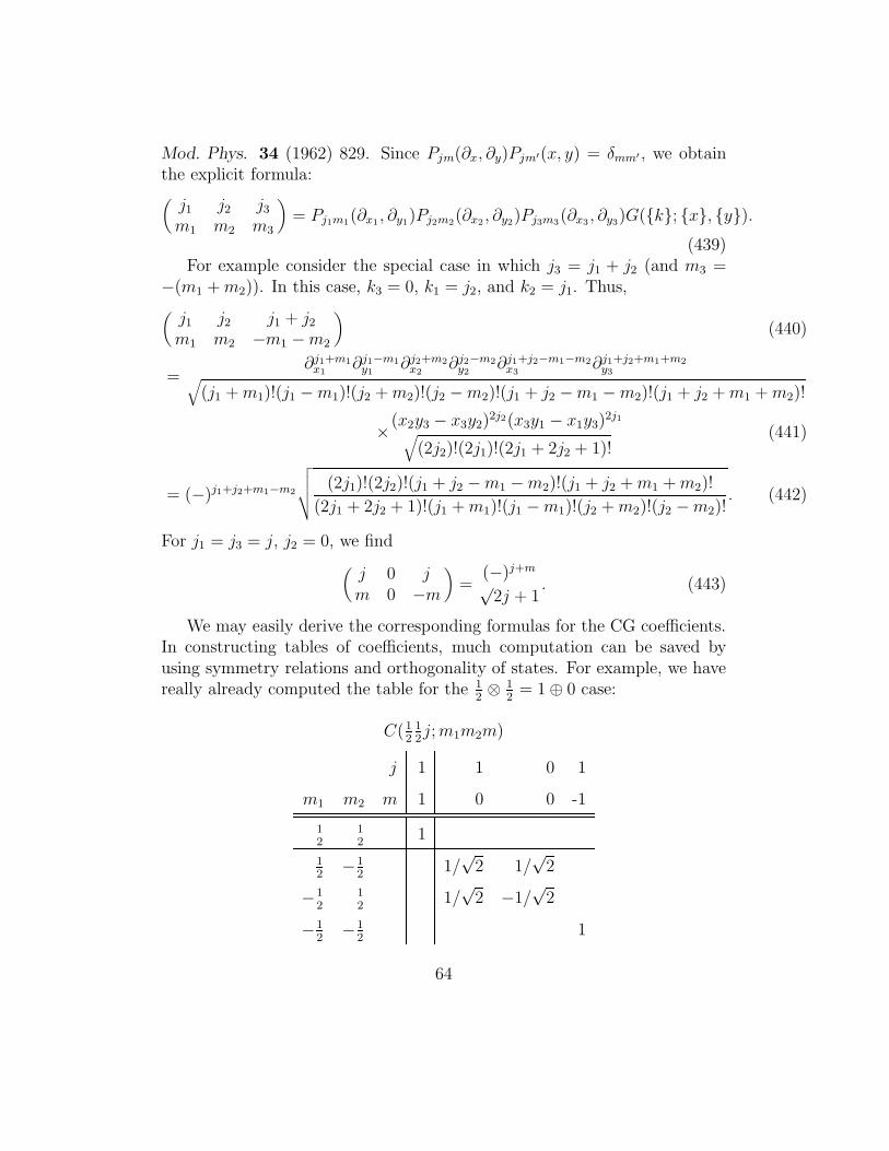
Mod. Phys. 34 (1962) 829. Since Pjm(∂x, ∂y)Pjm′(x, y) = δmm′ , we obtainthe explicit formula:(j1 j2 j3m1 m2 m3

)= Pj1m1(∂x1 , ∂y1)Pj2m2(∂x2 , ∂y2)Pj3m3(∂x3 , ∂y3)G(k; x, y).

(439)For example consider the special case in which j3 = j1 + j2 (and m3 =

−(m1 +m2)). In this case, k3 = 0, k1 = j2, and k2 = j1. Thus,(j1 j2 j1 + j2m1 m2 −m1 −m2

)(440)

=∂j1+m1x1

∂j1−m1y1

∂j2+m2x2

∂j2−m2y2

∂j1+j2−m1−m2x3

∂j1+j2+m1+m2y3√

(j1 +m1)!(j1 −m1)!(j2 +m2)!(j2 −m2)!(j1 + j2 −m1 −m2)!(j1 + j2 +m1 +m2)!

×(x2y3 − x3y2)2j2(x3y1 − x1y3)

2j1

√(2j2)!(2j1)!(2j1 + 2j2 + 1)!

(441)

= (−)j1+j2+m1−m2

√√√√ (2j1)!(2j2)!(j1 + j2 −m1 −m2)!(j1 + j2 +m1 +m2)!

(2j1 + 2j2 + 1)!(j1 +m1)!(j1 −m1)!(j2 +m2)!(j2 −m2)!. (442)

For j1 = j3 = j, j2 = 0, we find

(j 0 jm 0 −m

)=

(−)j+m√2j + 1

. (443)

We may easily derive the corresponding formulas for the CG coefficients.In constructing tables of coefficients, much computation can be saved byusing symmetry relations and orthogonality of states. For example, we havereally already computed the table for the 1

2⊗ 1

2= 1 ⊕ 0 case:

C(12

12j;m1m2m)

j 1 1 0 1

m1 m2 m 1 0 0 -1

12

12

1

12

−12

1/√

2 1/√

2

−12

12

1/√

2 −1/√

2

−12

−12

1

64

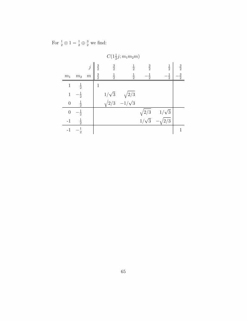
For 12⊗ 1 = 1

2⊕ 3

2we find:

C(112j;m1m2m)

j 32

32

12

32

12

32

m1 m2 m 32

12

12

−12

−12

−32

1 12

1

1 −12

1/√

3√

2/3

0 12

√2/3 −1/

√3

0 −12

√2/3 1/

√3

-1 12

1/√

3 −√

2/3

-1 −12

1

65

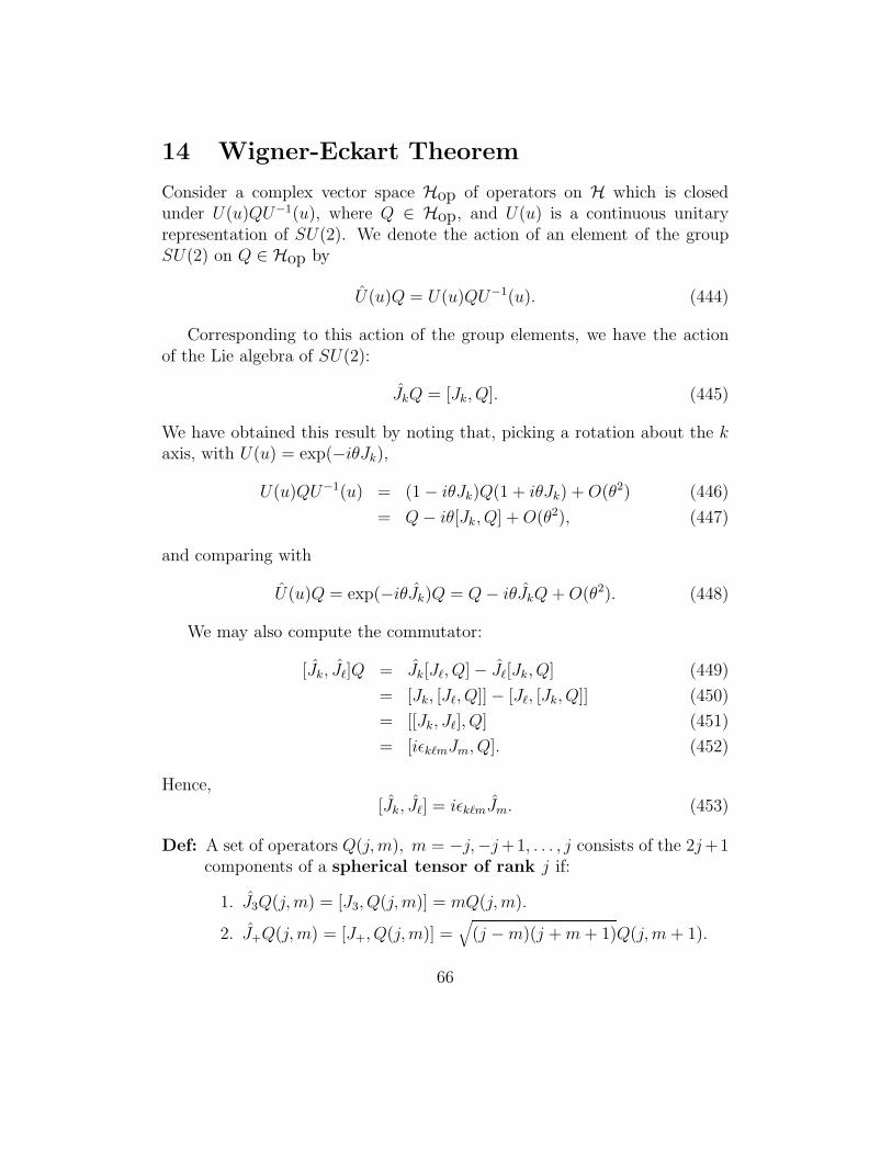
14 Wigner-Eckart Theorem

Consider a complex vector space Hop of operators on H which is closedunder U(u)QU−1(u), where Q ∈ Hop, and U(u) is a continuous unitaryrepresentation of SU(2). We denote the action of an element of the groupSU(2) on Q ∈ Hop by

U(u)Q = U(u)QU−1(u). (444)

Corresponding to this action of the group elements, we have the actionof the Lie algebra of SU(2):

JkQ = [Jk, Q]. (445)

We have obtained this result by noting that, picking a rotation about the kaxis, with U(u) = exp(−iθJk),

U(u)QU−1(u) = (1 − iθJk)Q(1 + iθJk) +O(θ2) (446)

= Q− iθ[Jk, Q] +O(θ2), (447)

and comparing with

U(u)Q = exp(−iθJk)Q = Q− iθJkQ +O(θ2). (448)

We may also compute the commutator:

[Jk, J`]Q = Jk[J`, Q] − J`[Jk, Q] (449)

= [Jk, [J`, Q]] − [J`, [Jk, Q]] (450)

= [[Jk, J`], Q] (451)

= [iεk`mJm, Q]. (452)

Hence,[Jk, J`] = iεk`mJm. (453)

Def: A set of operators Q(j,m), m = −j,−j+1, . . . , j consists of the 2j+1components of a spherical tensor of rank j if:

1. J3Q(j,m) = [J3, Q(j,m)] = mQ(j,m).

2. J+Q(j,m) = [J+, Q(j,m)] =√

(j −m)(j +m+ 1)Q(j,m + 1).

66

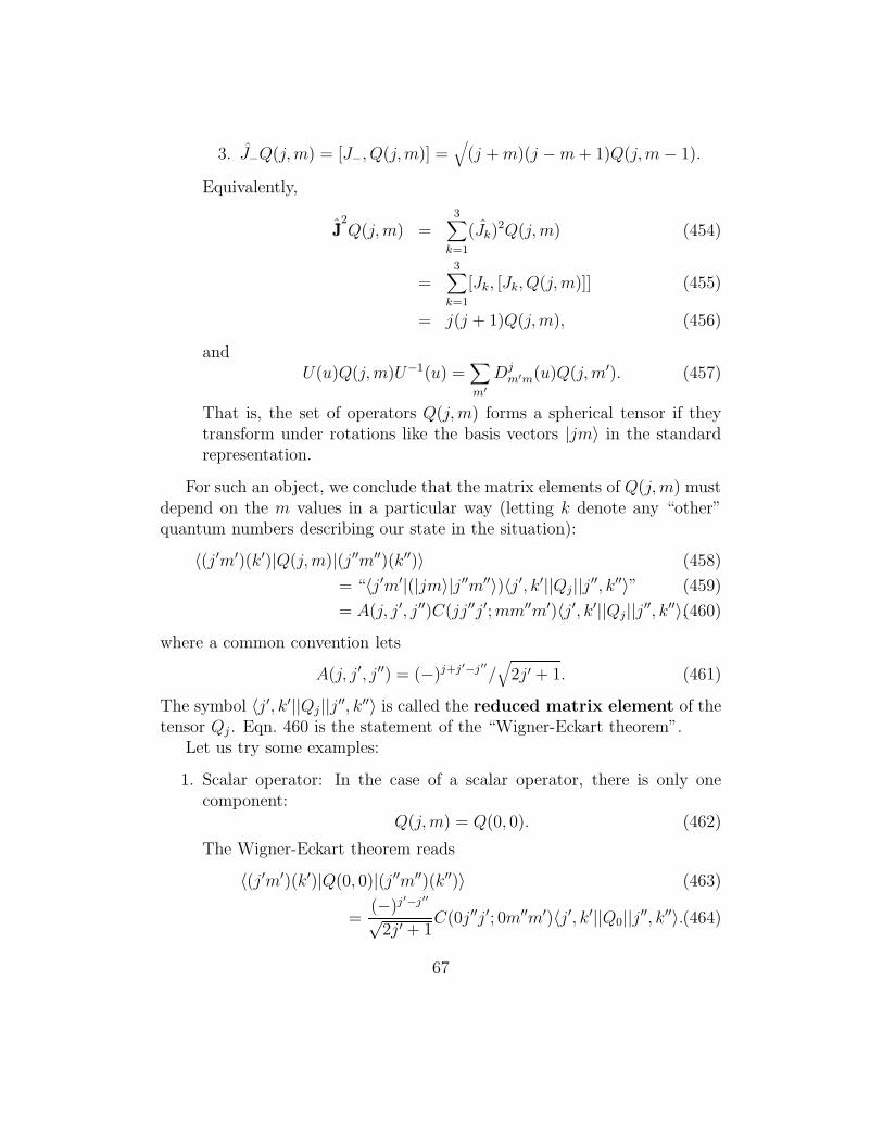
3. J−Q(j,m) = [J−, Q(j,m)] =√

(j +m)(j −m+ 1)Q(j,m− 1).

Equivalently,

JJJ2Q(j,m) =

3∑

k=1

(Jk)2Q(j,m) (454)

=3∑

k=1

[Jk, [Jk, Q(j,m)]] (455)

= j(j + 1)Q(j,m), (456)

andU(u)Q(j,m)U−1(u) =

∑

m′Djm′m(u)Q(j,m′). (457)

That is, the set of operators Q(j,m) forms a spherical tensor if theytransform under rotations like the basis vectors |jm〉 in the standardrepresentation.

For such an object, we conclude that the matrix elements of Q(j,m) mustdepend on the m values in a particular way (letting k denote any “other”quantum numbers describing our state in the situation):

〈(j ′m′)(k′)|Q(j,m)|(j ′′m′′)(k′′)〉 (458)

= “〈j ′m′|(|jm〉|j ′′m′′〉)〈j ′, k′||Qj||j ′′, k′′〉” (459)

= A(j, j ′, j ′′)C(jj ′′j ′;mm′′m′)〈j ′, k′||Qj||j ′′, k′′〉,(460)

where a common convention lets

A(j, j ′, j ′′) = (−)j+j′−j′′/

√2j ′ + 1. (461)

The symbol 〈j ′, k′||Qj||j ′′, k′′〉 is called the reduced matrix element of thetensor Qj. Eqn. 460 is the statement of the “Wigner-Eckart theorem”.

Let us try some examples:

1. Scalar operator: In the case of a scalar operator, there is only onecomponent:

Q(j,m) = Q(0, 0). (462)

The Wigner-Eckart theorem reads

〈(j ′m′)(k′)|Q(0, 0)|(j ′′m′′)(k′′)〉 (463)

=(−)j

′−j′′

√2j ′ + 1

C(0j ′′j ′; 0m′′m′)〈j ′, k′||Q0||j ′′, k′′〉.(464)

67

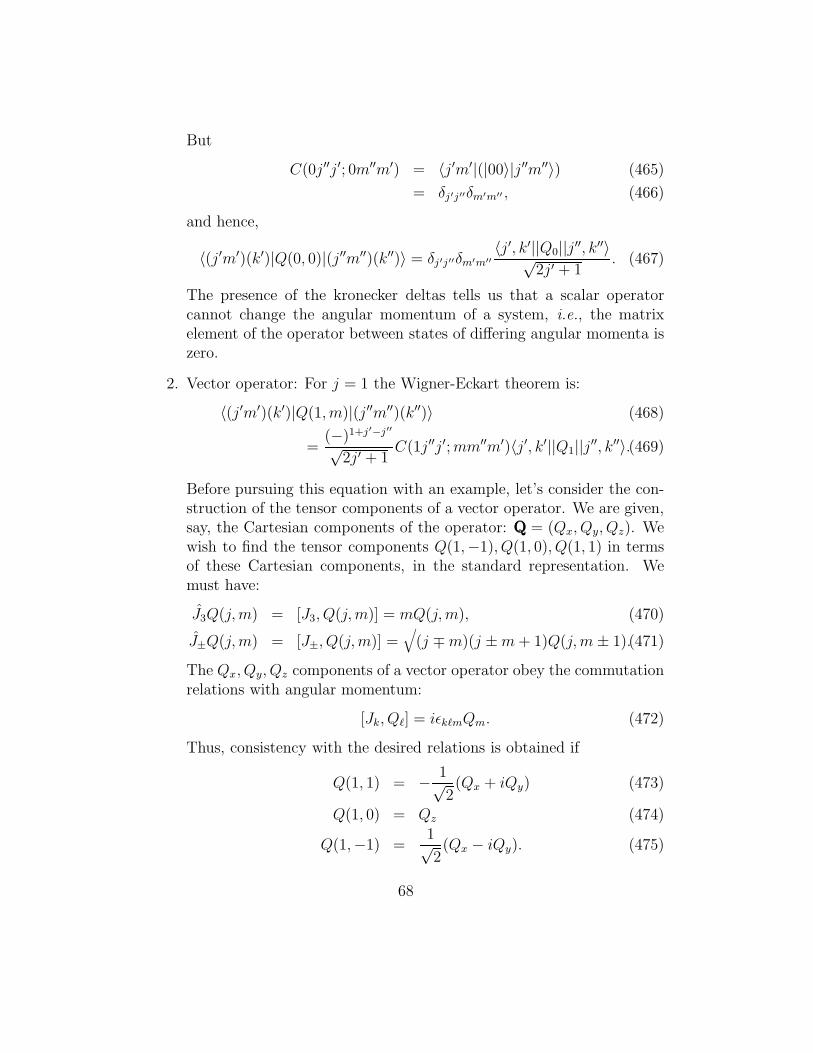
But

C(0j ′′j ′; 0m′′m′) = 〈j ′m′|(|00〉|j ′′m′′〉) (465)

= δj′j′′δm′m′′ , (466)

and hence,

〈(j ′m′)(k′)|Q(0, 0)|(j ′′m′′)(k′′)〉 = δj′j′′δm′m′′〈j ′, k′||Q0||j ′′, k′′〉√

2j ′ + 1. (467)

The presence of the kronecker deltas tells us that a scalar operatorcannot change the angular momentum of a system, i.e., the matrixelement of the operator between states of differing angular momenta iszero.

2. Vector operator: For j = 1 the Wigner-Eckart theorem is:

〈(j ′m′)(k′)|Q(1, m)|(j ′′m′′)(k′′)〉 (468)

=(−)1+j′−j′′

√2j ′ + 1

C(1j ′′j ′;mm′′m′)〈j ′, k′||Q1||j ′′, k′′〉.(469)

Before pursuing this equation with an example, let’s consider the con-struction of the tensor components of a vector operator. We are given,say, the Cartesian components of the operator: QQQ = (Qx, Qy, Qz). Wewish to find the tensor components Q(1,−1), Q(1, 0), Q(1, 1) in termsof these Cartesian components, in the standard representation. Wemust have:

J3Q(j,m) = [J3, Q(j,m)] = mQ(j,m), (470)

J±Q(j,m) = [J±, Q(j,m)] =√

(j ∓m)(j ±m+ 1)Q(j,m± 1).(471)

The Qx, Qy, Qz components of a vector operator obey the commutationrelations with angular momentum:

[Jk, Q`] = iεk`mQm. (472)

Thus, consistency with the desired relations is obtained if

Q(1, 1) = − 1√2(Qx + iQy) (473)

Q(1, 0) = Qz (474)

Q(1,−1) =1√2(Qx − iQy). (475)

68

These, then, are the components of a spherical tensor of rank 1, ex-pressed in terms of Cartesian components.

Now let’s consider the case where QQQ=JJJ, that is, the case in whichour vector operator is the angular momentum operator. To evaluatethe reduced matrix element, we chose any convenient component, forexample, Q(1, 0) = Jz. Hence,

〈j ′m′(k′)|Jz|j ′′m′′(k′′)〉 = δj′j′′δm′m′′δk′k′′m′′ (476)

=〈j ′, k′||J ||j ′′, k′′〉√

2j ′ + 1C(1j ′′j ′; 0m′′m′)(−)1+j′+j′′.(477)

We see that the reduced matrix element vanishes unless j ′ = j ′′ (andk′ = k′′).

The relevant CG coefficients are given by

C(1j ′j ′; 0m′m′) =√

2j ′ + 1(−)1−j′+m′(

1 j ′ j ′

0 m′ −m′

), (478)

where(

1 j ′ j ′

0 m′ −m′

)(479)

= P10(∂x1 , ∂y1)Pj′m′(∂x2 , ∂y2)Pj′,−m′(∂x3, ∂y3)G(k; x, y)(480)

= (−)j′−m′ 2m′

√(2j ′ + 2)(2j ′ + 1)2j ′

, (481)

which the reader is invited to demonstrate (with straightforward, thoughsomewhat tedious, algebra). Therefore,

C(1j ′j ′; 0m′m′) = − m′√j ′(j ′ + 1)

. (482)

Inserting the CG coefficients into our expression for the reduced matrixelement, we find

〈j ′, k′||J ||j ′′, k′′〉√2j ′ + 1

= δj′j′′δk′k′′√j ′(j ′ + 1). (483)

69

We see that this expression behaves like√〈JJJ2〉. Plugging back into the

Wigner-Eckart theorem, we find:

〈(j ′m′)(k′)|Jm|(j ′′m′′)(k′′)〉 (484)

= δj′j′′δk′k′′√j ′(j ′ + 1)[−C(1j ′j ′;mm′′m′)], (485)

where Jm = J1, J0, J−1 denotes the tensor components of JJJ.

Consider, for example, J(1, 1) = − 1√2J+. The Wigner-Eckart theorem

now tells us that

〈(jm+ 1| − 1√2J+|(jm)〉 = − 1√

2

√(j −m)(j +m + 1), (486)

=√j(j + 1)[−C(1jj; 1mm+ 1)].(487)

Thus, we have found an expression which may be employed to computesome CG coefficients:

C(1jj; 1mm+ 1) =

√√√√(j −m)(j +m+ 1)

2j(j + 1). (488)

We see that the Wigner-Eckart theorem applied to J itself can be usedto determine CG coefficients.

15 Exercises

1. Prove the theorem we state in this note:

Theorem: The most general mapping x → x′ of R3 into itself, suchthat the origin is mapped into the origin, and such that all dis-tances are preserved, is a linear, real orthogonal transformationQ:

x′ = Qx, where QTQ = I, and Q∗ = Q. (489)

Hence,x′ · y′ = x · y ∀ points x,y ∈ R3. (490)

For such a mapping, either:

70

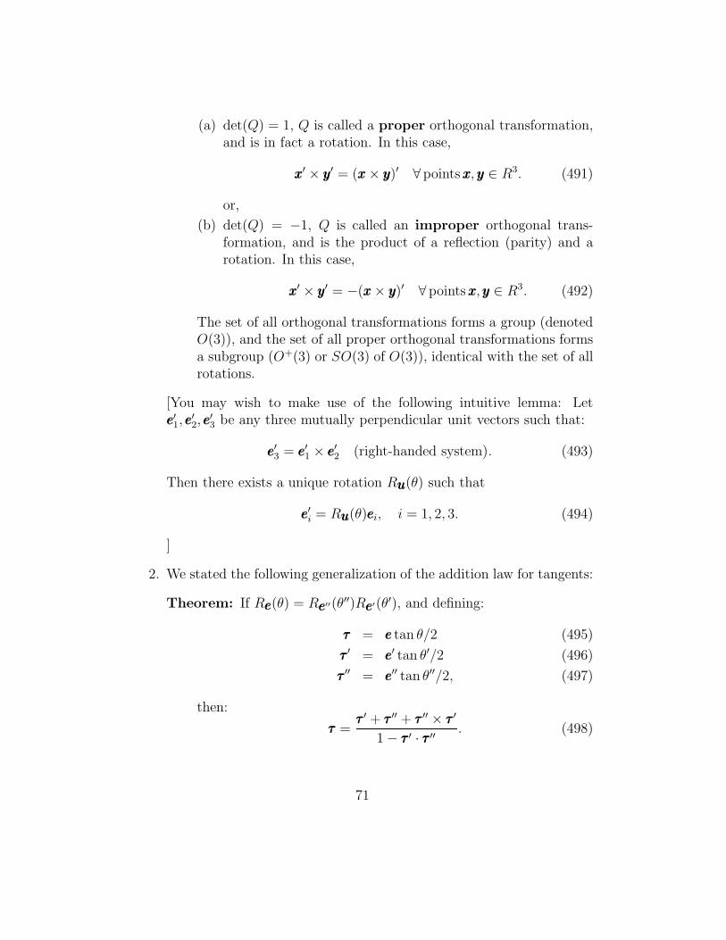
(a) det(Q) = 1, Q is called a proper orthogonal transformation,and is in fact a rotation. In this case,

xxx′ × yyy′ = (xxx× yyy)′ ∀ pointsxxx, yyy ∈ R3. (491)

or,

(b) det(Q) = −1, Q is called an improper orthogonal trans-formation, and is the product of a reflection (parity) and arotation. In this case,

xxx′ × yyy′ = −(xxx× yyy)′ ∀ pointsxxx, yyy ∈ R3. (492)

The set of all orthogonal transformations forms a group (denotedO(3)), and the set of all proper orthogonal transformations formsa subgroup (O+(3) or SO(3) of O(3)), identical with the set of allrotations.

[You may wish to make use of the following intuitive lemma: Leteee′1, eee

′2, eee

′3 be any three mutually perpendicular unit vectors such that:

eee′3 = eee′1 × eee′2 (right-handed system). (493)

Then there exists a unique rotation Ruuu(θ) such that

eee′i = Ruuu(θ)eeei, i = 1, 2, 3. (494)

]

2. We stated the following generalization of the addition law for tangents:

Theorem: If Reee(θ) = Reee′′(θ′′)Reee′(θ

′), and defining:

τττ = eee tan θ/2 (495)

τττ ′ = eee′ tan θ′/2 (496)

τττ ′′ = eee′′ tan θ′′/2, (497)

then:

τττ =τττ ′ + τττ ′′ + τττ ′′ × τττ ′

1 − τττ ′ · τττ ′′ . (498)

71

A simple way to prove this theorem is to use SU(2) to represent therotations, i.e., the rotation Reee(θ) is represented by the SU(2) matrix

exp(− i

2θeee · σ

). You are asked to carry out this proof.

3. We made the assertion that if we had an element u ∈ SU(2) whichcommuted with every element of the vector space of traceless 2 × 2Hermitian matrices, then u must be a multiple of the identity (i.e.,either u = I or u = −I). Let us demonstrate this, learning a littlemore group theory along the way.

First, we note that if we have a matrix group, it is possible to generateanother matrix representation of the group by replacing each elementwith another according to the mapping:

u → v (499)

wherev = SuS−1. (500)

and S is any chosen non-singular matrix.

(a) Show that if u is a matrix group, then v|v = SuS−1; S anon-singular matrix is a representation of the group (i.e., themapping is 1 : 1 and the multiplication table is preserved underthe mapping). The representations u and v are considered tobe equivalent.

A group of unitary matrices is said to be reducible if there ex-ists a mapping of the above form such that every element maysimultaneously be written in block-diagonal form:

M(g) =

A(g) 0 0

0 B(g) 0

0 0. . .

∀g ∈ the group (A(g) and B(g) are sub-matrices).

(b) Show that SU(2) is not reducible (i.e., SU(2) is irreducible).

(c) Now prove the following useful lemma: A matrix which commuteswith every element of an irreducible matrix group is a multiple ofthe identity matrix. [Hint: Let B be such a matrix commutingwith every element, and consider the eigenvector equation Bx =

72

λx. Then consider the vector ux where u is any element of thegroup, and x is the eigenvector corresponding to eigenvalue λ.]

(d) Finally, prove the assertion we stated at the beginning of thisproblem.

4. We have discussed rotations using the language of group theory. Let uslook at a simple application of group theory in determining “selectionrules” implied by symmetry under the elements of the group (wherethe group is a group of operations, such as rotations). The point isthat we can often predict much about the physics of a situation simplyby “symmetry” arguments, without resorting to a detailed solution.

Consider a positronium “atom”, i.e., the bound state of an electron anda positron. The relevant binding interaction here is electromagnetism.The electromagnetic interaction doesn’t depend on the orientation ofthe system, that is, it is invariant with respect to rotations. It alsois invariant with respect to reflections. You may wish to convinceyourself of these statements by writing down an explicit Hamiltonian,and verifying the invariance.

Thus, the Hamiltonian for positronium is invariant with respect tothe group O(3), and hence commutes with any element of this group.Hence, angular momentum and parity are conserved, and the eigen-states of energy are also eigenstates of parity and total angular mo-mentum (J). In fact, the spin and orbital angular momentum degreesof freedom are sufficiently decoupled that the total spin (S) and or-bital angular momentum (L) are also good quantum numbers for theenergy eigenstates to an excellent approximation. The ground stateof positronium (“parapositronium”) is the 1S0 state in 2S+1LJ spectro-scopic notation, where L = S means zero orbital angular momentum.Note that the letter “S” in the spectroscopic notation is not the sameas the “S” referring to the total spin quantum number. Sorry aboutthe confusion, but it’s established tradition. . .

In the ground state, the positron and electron have no relative orbitalangular momentum, and their spins are anti-parallel. The first excitedstate (“orthopositronium”) is the 3S1 state, in which the spins of thepositron and electron are now aligned parallel with each other. The3S1 −1 S0 splitting is very small, and is analogous to the “hyperfine”splitting in normal atoms.

73

Positronium decays when the electron and positron annihilate to pro-duce photons. The decay process is also electromagnetic, hence alsogoverned by a Hamiltonian which is invariant under O(3). As a conse-quence of this symmetry, angular momentum and parity are conservedin the decay.

(a) We said that parity was a good quantum number for positroniumstates. To say just what the parity is, we need to anticipate aresult from the Dirac equation (sorry): The intrinsic parities ofthe electron and positron are opposite. What is the parity ofparapositronium? Of orthopositronium?

(b) We wish to know whether positronium can decay into two photons.Let us check parity conservation. What are the possible paritiesof a state of two photons, in the center-of-mass frame? Can youexclude the decay of positronium to two photons on the basis ofparity conservation?

(c) Let us consider now whether rotational invariance, i.e., conserva-tion of angular momentum, puts any constraints on the permitteddecays of positronium. Can the orthopositronium state decay totwo photons? What about the parapositronium state?

5. The “charge conjugation” operator, C, is an operator that changes allparticles into their anti-particles. Consider the group of order 2 gen-erated by the charge conjugation operator. This group has elementsI, C, where I is the identity element. The electromagnetic interac-tion is invariant with respect to the actions of this group. That is, anyelectromagnetic process for a system of particles should proceed iden-tically if all the particles are replaced by their anti-particles. Hence, Cis a conserved quantity. Let’s consider the implications of this for the1S0 and 3S1 positronium decays to two photons. [See the preceedingexercise for a discussion of positronium. Note that you needn’t havedone that problem in order to do this one.]

(a) The result of operating C on a photon is to give a photon, i.e.,the photon is its own anti-particle, and is thus an eigenstate ofC. What is the eigenvalue? That is, what is the “C-parity” ofthe photon? You should give your reasoning. No credit will begiven for just writing down the answer, even if correct. [Hint:

74

think classically about electromagnetic fields and how they areproduced.] Hence, what is the C-parity of a system of n photons?

(b) It is a bit trickier to figure out the charge conjugation of thepositronium states. Since these are states consisting of a particleand its antiparticle, we suspect that they may also be eigenstatesof C. But is the eigenvalue positive or negative? To determinethis, we need to know a bit more than we know so far.

Let me give an heuristic argument for the new understanding thatwe need. First, although we haven’t talked about it yet, you prob-ably already know about the “Pauli Exclusion Principle”, whichstates that two identical fermions cannot be in the same state.

Suppose we have a state consisting of two electrons, |xxx1, SSS1;xxx2, SSS2〉.We may borrow an idea we introduced in our discussion of the har-monic oscillator, and define a “creation operator”, a†(xxx,SSS), whichcreates an electron at xxx with spin SSS. Consider the two-electronstate:

[a†(xxx1, SSS1)a†(xxx2, SSS2) + a†(xxx2, SSS2)a

†(xxx1, SSS1)]|0〉, (501)

where |0〉 is the “vacuum” state, with no electrons. But this putsboth electrons in the same state, since it is invariant under the in-terchange 1 ↔ 2. Therefore, in order to satisfy the Pauli principle,we must have that

a†(xxx1, SSS1)a†(xxx2, SSS2) + a†(xxx2, SSS2)a

†(xxx1, SSS1) = 0 (502)

That is, the creation operators anti-commute. To put it an-other way, if two electrons are interchanged, a minus sign is in-troduced. You may be concerned that a positron and an electronare non-identical particles, so maybe this has nothing to do withpositronium. However, the relativistic description is such that thepositron and electron may be regarded as different “components”of the electron (e.g., the positron may be interpreted in terms of“negative-energy” electron states), so this anti-commutation rela-tion is preserved even when creating electrons and positrons.

Determine the C-parity of the 3S1 and 1S0 states of positronium,and thus deduce whether decays to two photons are permittedaccording to conservation of C. [Hint: Consider a positronium

75

state and let C act on it. Relate this back to the original state byappropriate transformations.]

6. Suppose we have a system with total angular momentum 1. We picka basis corresponding to the three eigenvectors of the z-component ofangular momentum, Jz, with eigenvalues +1, 0,−1, respectively. Weare given an ensemble described by density matrix:

ρ =1

4

2 1 11 1 01 0 1

.

(a) Is ρ a permissible density matrix? Give your reasoning. For theremainder of this problem, assume that it is permissible. Does itdescribe a pure or mixed state? Give your reasoning.

(b) Given the ensemble described by ρ, what is the average value ofJz?

(c) What is the spread (standard deviation) in measured values of Jz?

7. Let us consider the application of the density matrix formalism to theproblem of a spin-1/2 particle (such as an electron) in a static externalmagnetic field. In general, a particle with spin may carry a magneticmoment, oriented along the spin direction (by symmetry). For spin-1/2, we have that the magnetic moment (operator) is thus of the form:

µµµ =1

2γσσσ, (503)

where σσσ are the Pauli matrices, the 12

is by convention, and γ is aconstant, giving the strength of the moment, called the gyromagneticratio. The term in the Hamiltonian for such a magnetic moment in anexternal magnetic field, BBB is just:

H = −µµµ ·BBB. (504)

Our spin-1/2 particle may have some spin-orientation, or “polarizationvector”, given by:

PPP = 〈σσσ〉. (505)

76

Drawing from our classical intuition, we might expect that in the ex-ternal magnetic field the polarization vector will exhibit a precessionabout the field direction. Let us investigate this.

Recall that the expectation value of an operator may be computed fromthe density matrix according to:

〈A〉 = Tr(ρA). (506)

Furthermore, recall that the time evolution of the density matrix isgiven by:

i∂ρ

∂t= [H(t), ρ(t)]. (507)

What is the time evolution, dP/dt, of the polarization vector? Expressyour answer as simply as you can (more credit will be given for rightanswers that are more physically transparent than for right answerswhich are not). Note that we make no assumption concerning thepurity of the state.

8. Let us consider a system of N spin-1/2 particles (as in the previousproblem) per unit volume in thermal equilibrium, in our external mag-netic field B. [Even though we refer to the previous exercise, the solu-tion to this problem does not require solving the previous one.] Recallthat the canonical distribution is:

ρ =e−H/T

Z, (508)

with partition function:

Z = Tr(e−H/T

). (509)

Such a system of particles will tend to orient along the magnetic field,resulting in a bulk magnetization (having units of magnetic momentper unit volume), M.

(a) Give an expression for this magnetization (don’t work too hard toevaluate).

(b) What is the magnetization in the high-temperature limit, to lowestnon-trivial order (this I want you to evaluate as completely as youcan!)?

77

9. We have discussed Lie algrebras (with Lie product given by the com-mutator) and Lie groups, in our attempt to deal with rotations. At onepoint, we asserted that the structure (multiplication table) of the Liegroup in some neighborhood of the identity was completely determinedby the structure (multiplication table) of the Lie algebra. We notedthat, however intuitively pleasing this might sound, it was not actuallya trivial statement, and that it followed from the “Baker-Campbell-Hausdorff” theorem. Let’s try to tidy this up a bit further here.

First, let’s set up some notation: Let L be a Lie algebra, and G be theLie group generated by this algebra. Let X, Y ∈ L be two elements ofthe algebra. These generate the elements eX , eY ∈ G of the Lie group.We assume the notion that if X and Y are close to the zero element ofthe Lie algebra, then eX and eY will be close to the identity element ofthe Lie group.

What we want to show is that the group product eXeY may be ex-pressed in the form eZ , where Z ∈ L, at least for X and Y not too“large”. Note that the non-trivial aspect of this problem is that, first,X and Y may not commute, and second, objects of the form XY maynot be in the Lie algebra. Elements of L generated by X and Y mustbe linear combinations of X, Y , and their repeated commutators.

(a) Suppose X and Y commute. Show explicitly that the producteXeY is of the form eZ, where Z is an element of L. (If you thinkthis is trivial, don’t worry, it is!)

(b) Now suppose that X and Y may not commute, but that they arevery close to the zero element. Keeping terms to quadratic orderin X and Y , show once again that the product eXeY is of the formeZ , where Z is an element of L. Give an explicit expression for Z.

(c) Finally, for more of a challenge, let’s do the general theorem: Showthat eXeY is of the form eZ , where Z is an element of L, as longas X and Y are sufficiently “small”. We won’t concern ourselveshere with how “small” X and Y need to be – you may investigatethat at more leisure.

Here are some hints that may help you: First, we remark that thedifferential equation

df

du= Xf(u) + g(u), (510)

78

where X ∈ L, and letting f(0) = f0, has the solution:

f(u) = euXf0 +∫ u

0e(u−v)Xg(v)dv. (511)

This can be readily verified by back-substitution. If g is indepen-dent of u, then the integral may be performed, with the result:

f(u) = euXf0 + h(u,X)g, (512)

Where, formally,

h(u,X) =euX − 1

X. (513)

Second, if X, Y ∈ L, then

eXY e−X = eXc(Y ), (514)

where I have introduced the notation “Xc” to mean “take thecommutator”. That is, Xc(Y ) ≡ [X, Y ]. This fact may be demon-strated by taking the derivative of

A(u;Y ) ≡ euXY e−uX (515)

with respect to u, and comparing with our differential equationabove to obtain the desired result.

Third, assuming X = X(u) is differentiable, we have

eX(u) d

due−X(u) = −h(1, X(u)c)

dX

du. (516)

This fact may be verified by considering the object:

B(t, u) ≡ etX(u) ∂

∂ue−tX(u), (517)

and differentiating (carefully!) with respect to t, using the abovetwo facts, and finally letting t = 1.

One final hint: Consider the quantity

Z(u) = ln(euXeY

). (518)

The series:

`(z) =ln z

z − 1= 1 − z − 1

2+

(z − 1)2

3− · · · (519)

plays a role in the explicit form for the result. Again, you are notasked to worry about convergence issues.

79

10. In an earlier exercise we considered the implication of rotational in-variance for the decays of positronium states into two photons. Let usgeneralize and broaden that discussion here. Certain neutral particles(e.g., π0, η, η′) are observed to decay into two photons, and others (e.g.,ω, φ, ψ) are not. Let us investigate the selection rules implied by an-gular momentum and parity conservation (satisfied by electromagneticand strong interactions) for the decay of a particle (call it “X”) intotwo photons. Thus, we ask the question, what angular momentum Jand parity P states are allowed for two photons?

Set up the problem in the center-of-mass frame of the two photons,with the z-axis in the direction of one photon. We know that since aphoton is a massless spin-one particle, it has two possible spin states,which we can describe by its “helicity”, i.e., its spin projection along itsdirection of motion, which can take on the values ±1. Thus, a systemof two photons can have the spin states:

|↑↑〉, |↓↓〉, |↑↓ + ↓↑〉, |↑↓ − ↓↑〉

(The first arrow refers to the photon in the +z direction, the secondto the photon in the −z direction, and the direction of the arrow in-dicates the spin component along the z-axis, NOT to the helicity.)We consider the effect on these states of three operations (which, byparity and angular momentum conservation, should commute with theHamiltonian):

• P : parity – reverses direction of motion of a particle, but leavesits angular momentum unaltered.

• Rz(α): rotation by angle α about the z-axis. A state with a givenvalue of Jz (z-component of angular momentum) is an eigenstate,with eigenvalue eiαJz .

• Rx(π): rotation by π about x-axis. For our two photons, thisreverses the direction of motion and also the angular momentumof each photon. For our “X” particle, this operation has the effectcorresponding to the effect on the spherical harmonic with theappropriate eigenvalues:

Rx(π)YJJz(Ω)

80

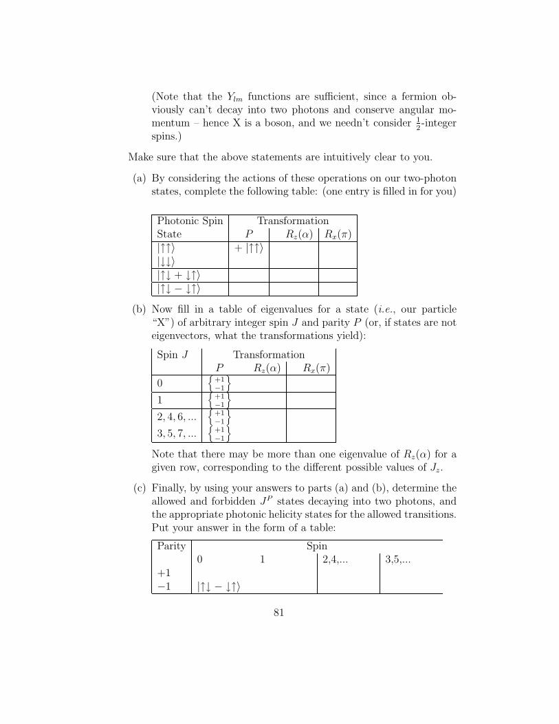
(Note that the Ylm functions are sufficient, since a fermion ob-viously can’t decay into two photons and conserve angular mo-mentum – hence X is a boson, and we needn’t consider 1

2-integer

spins.)

Make sure that the above statements are intuitively clear to you.

(a) By considering the actions of these operations on our two-photonstates, complete the following table: (one entry is filled in for you)

Photonic Spin TransformationState P Rz(α) Rx(π)|↑↑〉 + |↑↑〉|↓↓〉|↑↓ + ↓↑〉|↑↓ − ↓↑〉

(b) Now fill in a table of eigenvalues for a state (i.e., our particle“X”) of arbitrary integer spin J and parity P (or, if states are noteigenvectors, what the transformations yield):

Spin J TransformationP Rz(α) Rx(π)

0

+1−1

1

+1−1

2, 4, 6, ...

+1−1

3, 5, 7, ...

+1−1

Note that there may be more than one eigenvalue of Rz(α) for agiven row, corresponding to the different possible values of Jz.

(c) Finally, by using your answers to parts (a) and (b), determine theallowed and forbidden JP states decaying into two photons, andthe appropriate photonic helicity states for the allowed transitions.Put your answer in the form of a table:

Parity Spin0 1 2,4,... 3,5,...

+1−1 |↑↓ − ↓↑〉

81

You have (I hope) just derived something which is often referred to as“Yang’s theorem”. Note: People often get this wrong, so be careful!

11. We said that if we are given an arbitrary representation, D(u), ofSU(2), it may be reduced to a direct sum of irreps Dr(u):

D(u) =∑

r

⊕Dr(u). (520)

The multiplicities mj (the number of irreducible representations Dr

which belong to the equivalence class of irreducible representationscharacterized by index j) are unique, and they are given by:

mj =∫

SU(2)d(u)χj(u−1)χ(u), (521)

where χ(u) = Tr [D(u)].

(a) Suppose you are given a representation, with characters:

χ [ueee(θ)] = 1 +sin 3

2θ + 2 sin 7

4θ cos 1

4θ

sin 12θ

. (522)

What irreducible representations appear in the reduction of thisrepresentation, with what multiplicities?

(b) Does the representation we are given look like it could correspondto rotations of a physically realizable system? Discuss.

12. In nuclear physics, we have the notion of “charge independence”, orthe idea that the nuclear (strong) force does not depend on whetherwe are dealing with neutrons or protons. Thus, the nuclear force issupposed to be symmetric with respect to unitary transformations ona space with basis vectors p =

(10

), n =

(01

). Neglecting the overall

phase symmetry, we see that the symmetry group is SU(2), just as forrotations. As with angular momentum, we can generate representationsof other dimensions, and work with systems of more than one nucleon.By analogy with angular momentum, we say that the neutron andproton form an “isotopic spin” (or “isospin”) doublet, with

|n〉 = |I =1

2, I3 = −1

2〉 (523)

|p〉 = |I =1

2, I3 = +

1

2〉 (524)

82

(The symbol “T” is also often used for isospin). Everything you knowabout SU(2) can now be applied in isotopic spin space.

Study the isobar level diagram of the He6,Li6,Be6 nuclear level schemes,and discuss in detail the evidence for charge independence of the nu-clear force. These graphs are quantitative, so your discussion shouldalso be quantitative. Also, since these are real-life physical systems,you should worry about real-life effects which can modify an idealizedvision.

You may find an appropriate level scheme via a google search (you wanta level diagram for the nuclear isobars of 6 nucleons), e.g., at:http://www.tunl.duke.edu/nucldata/figures/06figs/06 is.pdfFor additional reference, you might find it of interest to look up:F. Ajzenberg-Selove, “Energy Levels of Light Nuclei, A = 5-10,” Nucl.Phys. A490 1-225 (1988)(see also http://www.tunl.duke.edu/nucldata/fas/88AJ01.shtml).

13. We defined the “little-d” functions according to:

djm1m2(θ) = Dj

m1m2(0, θ, 0) = 〈j,m1|e−iθJ2|j,m2〉

where the matrix elements Djm1m2

(ψ, θ, φ), parameterized by Euler an-gles ψ, θ, φ, are given in the “standard representation” by:

Djm1m2

(ψ, θ, φ) = 〈j,m1|Dj(u)|j,m2〉 = e−i(m1ψ+m2φ)djm1m2(θ)

We note that an explicit calculation for these matrix elements is pos-sible via:

Djm1m2

(u) = Pjm1(∂x, ∂y)Pjm2(u11x + u21y, u12x + u22y) (525)

where

Pjm(x, y) ≡ xj+myj−m√(j +m)!(j −m)!

. (526)

Prove the following handy formulas for the djm1m2(θ) functions:

a) dj∗m1m2(θ) = djm1m2

(θ) (reality of dj functions)

b) djm1m2(−θ) = djm2m1

(θ)

83

c) djm1m2(θ) = (−)m1−m2djm2m1

(θ)

d) dj−m1,−m2(θ) = (−)m1−m2djm1m2

(θ)

e) djm1m2(π − θ) = (−)j−m2dj−m1,m2

(θ) = (−)j+m1djm1,−m2(θ)

f) djm1m2(2π + θ) = (−)2jdjm1m2

(θ)

14. We would like to consider the (qualitative) effects on the energy levelsof an atom which is moved from freedom to an external potential (acrystal, say) with cubic symmetry. Let us consider a one-electron atomand ignore spin for simplicity. Recall that the wave function for thecase of the free atom looks something like Rnl(r)Ylm(θ, φ), and thatall states with the same n and l quantum numbers have the sameenergy, i .e., are (2l + 1)-fold degenerate. The Hamiltonian for a freeatom must have the symmetry of the full rotation group, as there areno special directions. Thus, we recall some properties of this groupfor the present discussion. First, we remark that the set of functionsYlm : m = −l,−l + 1, · · · , l − 1, l for a given l forms the basis for a(2l + l)-dimensional subspace which is invariant under the operationsof the full rotation group. [A set ψi of vectors is said to span aninvariant subspace Vs under a given set of operations Pj if Pjψi ∈ Vs∀i, j.] Furthermore, this subspace is “irreducible,” that is, it cannot besplit into smaller subspaces which are also invariant under the rotationgroup.

Let us denote the linear transformation operator corresponding to ele-ment R of the rotation group by the symbol PR, i.e.:

PRf(~x) = f(R−1~x)

84

The way to think about this equation is to regard the left side as givinga “rotated function,” which we evaluate at point ~x. The right side tellsus that this is the same as the original function evaluated at the pointR−1~x, where R−1 is the inverse of the rotation matrix corresponding torotation R. Since Ylm forms an invariant subspace, we must have:

PRYlm =l∑

m′=−1

Ylm′Dl(R)m′m

The expansion coefficients, Dl(R)m′m, can be regarded as the elementsof a matrix Dl(R). As discussed in the note, D` corresponds to anirreducible representation of the rotation group.

Thus, for a free atom, we have that the degenerate eigenfunctions ofa given energy must transform according to an irreducible representa-tion of this group. If the eigenfunctions transform according to the lth

representation, the degeneracy of the energy level is (2l+1) (assumingno additional, “accidental” degeneracy).

I remind you of the following:

Definition: Two elements a and b of a group are said to belong to thesame “class” (or “equivalence class” or “conjugate class”) if there existsa group element g such that g−1ag = b.

The first two parts of this problem, are really already done in the note,but here is an opportunity to think about it for yourself:

(a) Show that all proper rotations through the same angle ϕ, aboutany axis, belong to the same class of the rotation group.

(b) We will need the character table of this group. Since all elementsin the same class have the same character, we pick a convenientelement in each class by considering rotations about the z-axis,R = (α, z) (means rotate by angle α about the z-axis). Thus:

P(α,z)Y`m = e−imαY`m

(which you should convince yourself of).

Find the character “table” of the rotation group, that is, findχ`(α), the character of representation D` for the class of rotationsthrough angle α. If you find an expression for the character in the

85

form of a sum, do the sum, expressing your answer in as simple aform as you can.

(c) At last we are ready to put our atom into a potential with cubicsymmetry. Now the symmetry of the free Hamiltonian is broken,and we are left with the discrete symmetry of the cube. Thesymmetry group of proper rotations of the cube is a group oforder 24 with 5 classes. Call this group “O”.

Construct the character table for O.

(d) Consider in particular how the f -level (l = 3) of the free atommay split when it is placed in the “cubic potential”. The seveneigenfunctions which transform according to the irreducible rep-resentation D3 of the full group will most likely not transformaccording to an irreducible representation of O. On the otherhand, since the operations of O are certainly operations of D, theeigenfunctions will generate some representation of O.

Determine the coefficients in the decomposition.

D3 = a1O1 ⊕ a2O

2 ⊕ a3O3 ⊕ a4O

4 ⊕ a5O5,

where Oi are the irreducible representations of O. Hence, showhow the degeneracy of the 7-fold level may be reduced by the cubicpotential. Give the degeneracies of the final levels.

Note that we cannot say anything here about the magnitude ofany splittings (which could “accidentally” turn out to be zero!),or even about the ordering of the resulting levels – that dependson the details of the potential, not just its symmetry.

15. We perform an experiment in which we shine a beam of unpolarizedwhite light at a gas of excited hydrogen atoms. We label atomic statesby |n`m〉, where ` is the total (orbital, we are neglecting spin in thisproblem) angular momentum, m is the z-component of angular momen-tum (Lz|n`m〉 = m|n`m〉), and n is a quantum number determiningthe radial wave function. The light beam is shone along the x-axis.

We are interested in transition rates between atomic states, induced bythe light. Since we are dealing with visible light, its wavelength is muchlarger than the size of the atom. Thus, it is a good first approximationto consider only the interaction of the atomic dipole moment with the

86

electric field of the light beam. That is, the spatial variation in theplane wave eikx, describing the light beam, may be replaced by thelowest-order term in its expansion, i.e., by 1. Thus, we need onlyconsider the interaction of the dipole moment with the electric field ofthe light beam, taken to be uniform. The electric dipole moment ofthe atom is proportional to exxx, where xxx is the position of the electronrelative to the nucleus. Hence, in the “dipole approximation”, we areinterested in matrix elements of xxx ·EEE, where EEE is the electric field vectorof the light beam.

Calculate the following ratios of transition rates in the dipole approxi-mation:

a)Γ(|23, 1, 1〉 → |1, 0, 0〉)Γ(|23, 1, 0〉 → |1, 0, 0〉)

b).Γ(|3, 1, 0〉 → |4, 2, 1〉)

Γ(|3, 1,−1〉 → |4, 2, 0〉)

[Hint: this is an application of the Wigner-Eckart theorem.]

16. It is possible to arrive at the Clebsch-Gordan coefficients for a givensituation by “elementary” means, i.e., by considering the action of theraising and lowering operators and demanding orthonormality. Hence,construct a table of Clebsch-Gordan coefficients, using this approach,for a system combining j1 = 2 and j2 = 1 angular momenta. I find itconvenient to use the simple notation |jm〉 for total quantum numbersand |j1m1〉|j2m2〉 for the individual angular momentum states beingadded, but you may use whatever notation you find convenient.] Youwill find (I hope) that you have the freedom to pick certain signs. Youare asked to be consistent with the usual conventions where

〈33| (|22〉|11〉) ≥ 0 (527)

〈22| (|22〉|10〉) ≥ 0 (528)

〈11| (|22〉|1−1〉) ≥ 0 (529)

(in notation 〈jm| (|j1m1〉|j2m2〉)).

87

17. In our discussion of the Wigner-Eckart theorem, we obtained the re-duced matrix element for the angular momentum operator: 〈j ′k′‖J‖j ′′k′′〉.This required knowing the Clebsch-Gordan coefficient C(1, j, j; 0, m,m).By using the general prescription for calculating the 3j symbols we de-veloped, calculate the 3j symbol

(1 j j0 m −m

),

and hence obtain C(1, j, j; 0, m,m).

18. Rotational Invariance and angular distributions: A spin-1 particle ispolarized such that its spin direction is along the +z axis. It decays,with total decay rate Γ, to π+π−. What is the angular distribution,dΓ/dΩ, of the π+? Note that the π± is spin zero. What is the angulardistribution if the intial spin projection is zero along the z-axis? Minusone? What is the result if the intial particle is unpolarized (equalprobabilities for all spin orientations)?

19. Here is another example of how we can use the rotation matrices tocompute the angular distribution in a decay process. Let’s try anothersimilar example. Consider a spin one particle, polarized with its angularmomentum along the ±z-axis, with equal probabilities. Suppose itdecays to two spin-1/2 particles, e.g., an electron and a positron.

(a) Such the decay occurs with no orbital angular momentum. Whatis the angular distribution of the decay products, in the frame ofthe decaying particle?

(b) If this is an electromagnetic decay to e+e−, and the mass of thedecaying particle is much larger than the electron mass, the sit-uation is altered, according to relativistic QED. In this case, thefinal state spins will be oriented in such a way as to give eitherm = 1 or m = −1 along the decay axis, where m is the totalprojected angular momentum. What is the angular distributionof the decay products in this case?

88