1

Numerical Algorithms

• Matrix multiplication

• Solving a system of linear equations

ITCS 4/5145 Parallel Computing UNC-Charlotte, B. Wilkinson, Feb 28, 2012.

2

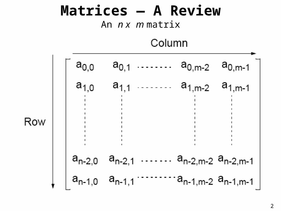
Matrices — A ReviewAn n x m matrix

3

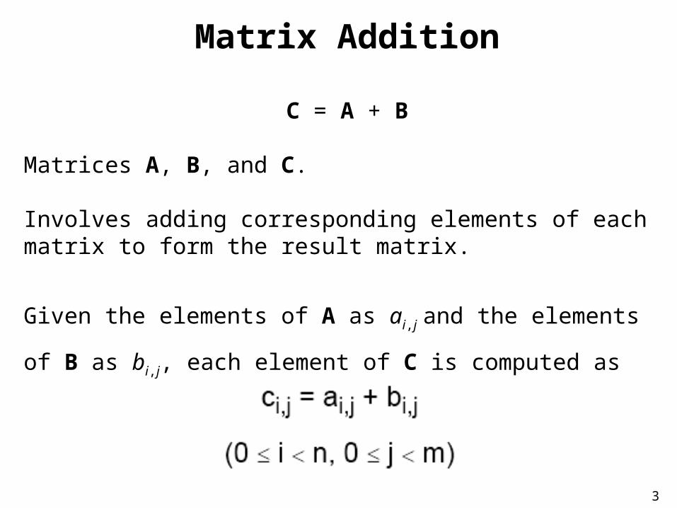
Matrix Addition

C = A + B

Matrices A, B, and C.

Involves adding corresponding elements of each matrix to form the result matrix.

Given the elements of A as ai,j and the elements of B as bi,j,

each element of C is computed as

4

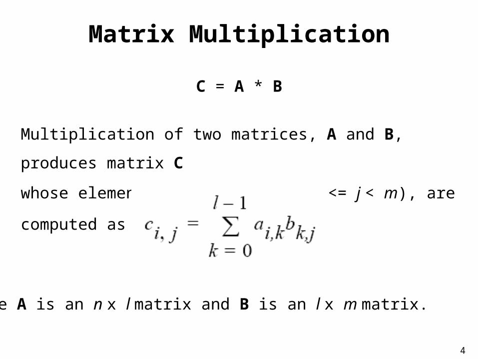
Matrix Multiplication

C = A * B

Multiplication of two matrices, A and B, produces matrix C

whose elements, ci,j (0 <= i < n, 0 <= j < m), are computed as

follows:

where A is an n x l matrix and B is an l x m matrix.

5

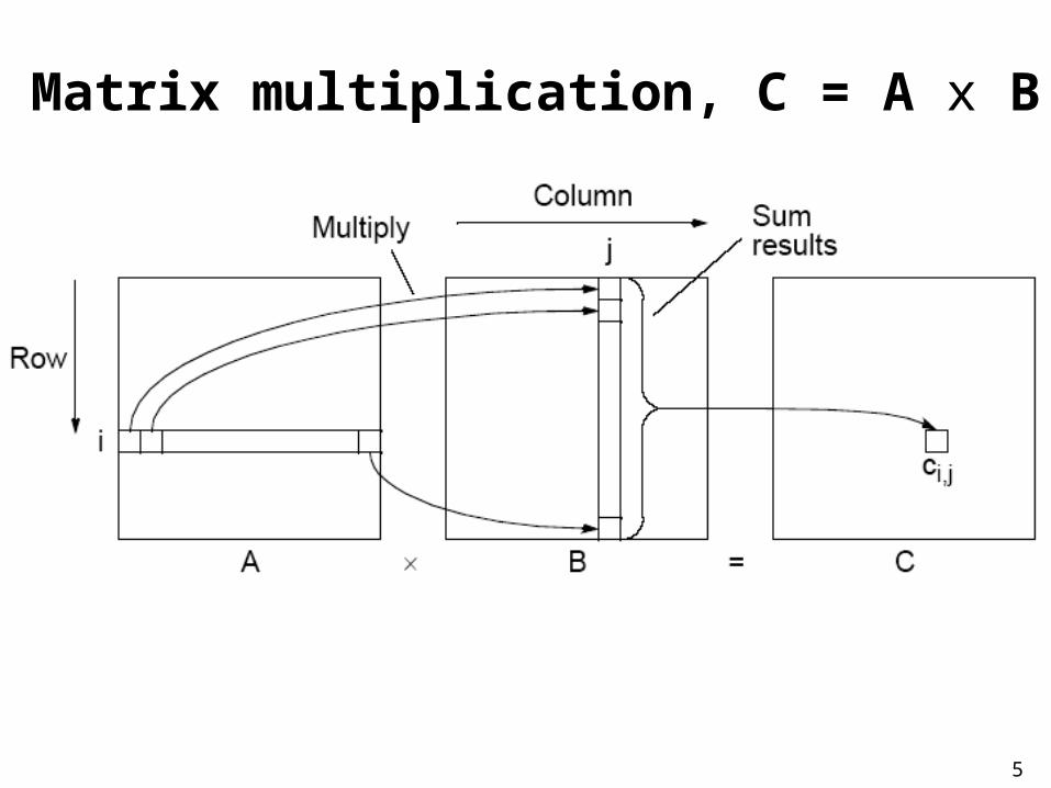
Matrix multiplication, C = A x B

6

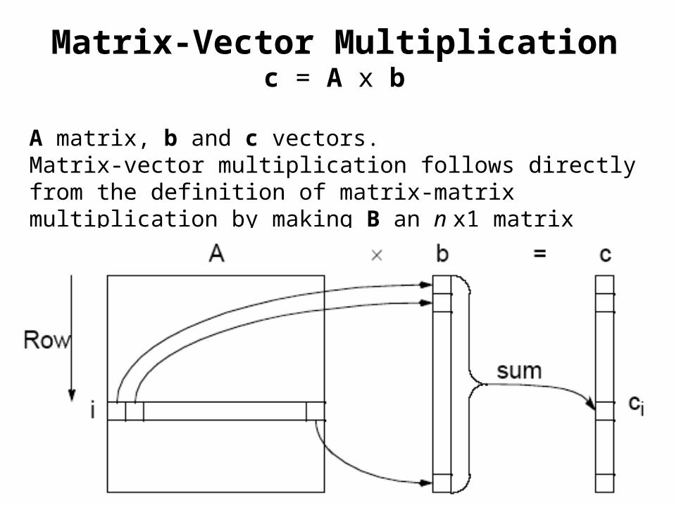
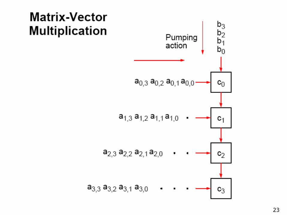
Matrix-Vector Multiplicationc = A x b

A matrix, b and c vectors.Matrix-vector multiplication follows directly from the definition of matrix-matrix multiplication by making B an n x1 matrix (vector). Result an n x 1 matrix (vector).

7

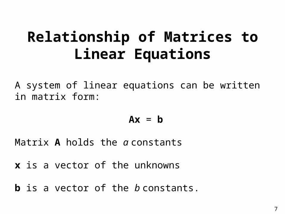
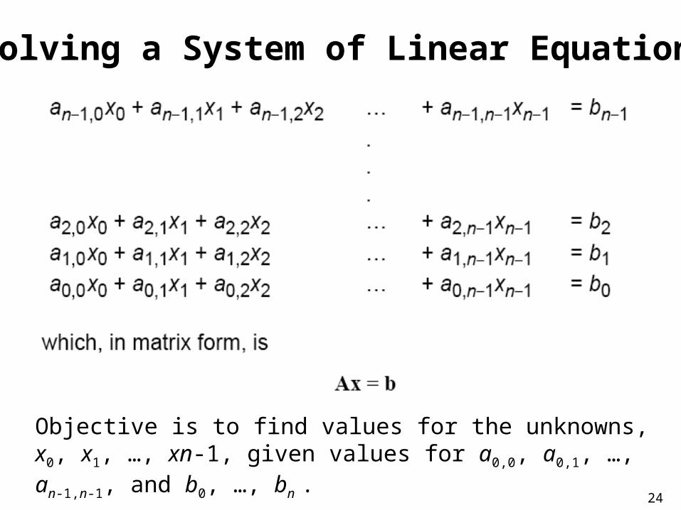
Relationship of Matrices to Linear Equations

A system of linear equations can be written in matrix form:

Ax = b

Matrix A holds the a constants

x is a vector of the unknowns

b is a vector of the b constants.

8

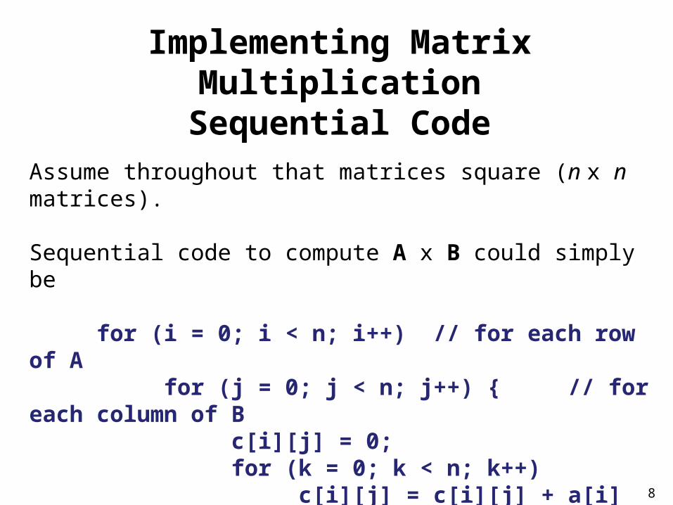
Implementing Matrix MultiplicationSequential Code

Assume throughout that matrices square (n x n matrices).

Sequential code to compute A x B could simply be

for (i = 0; i < n; i++) // for each row of Afor (j = 0; j < n; j++) { // for each column

of Bc[i][j] = 0;for (k = 0; k < n; k++)

c[i][j] = c[i][j] + a[i][k] * b[k][j];}

Requires n3 multiplications and n3 additionsSequential time complexity of O(n3). Very easy to parallelize.

9

Parallel Code

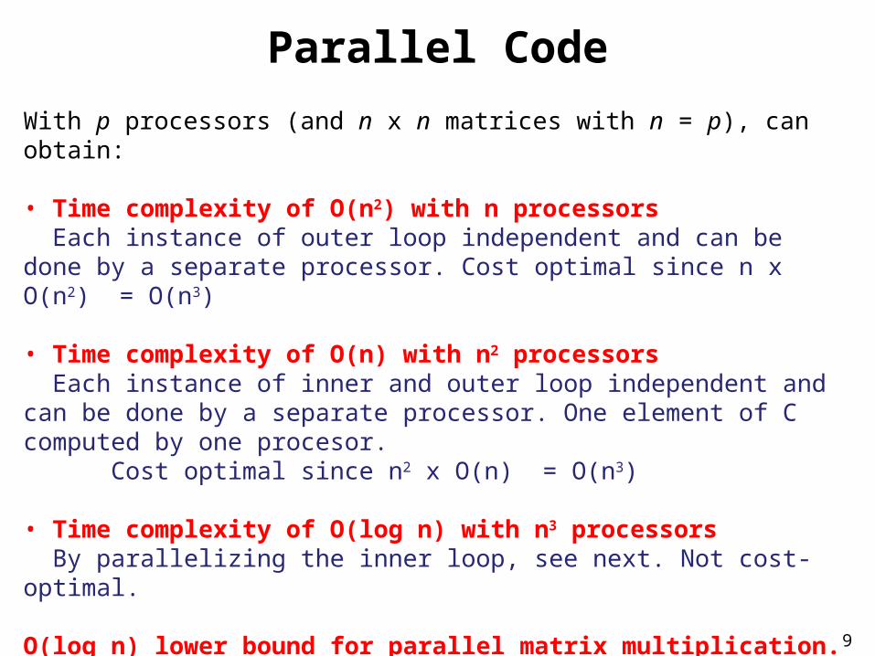
With p processors (and n x n matrices with n = p), can obtain:

• Time complexity of O(n2) with n processors Each instance of outer loop independent and can be done by a separate processor. Cost optimal since n x O(n2) = O(n3)

• Time complexity of O(n) with n2 processors Each instance of inner and outer loop independent and can be done by a separate processor. One element of C computed by one procesor.

Cost optimal since n2 x O(n) = O(n3)

• Time complexity of O(log n) with n3 processors By parallelizing the inner loop, see next. Not cost-optimal.

O(log n) lower bound for parallel matrix multiplication.

Cost-optimal: when time complexity x no of processors same as sequential time complexity

10

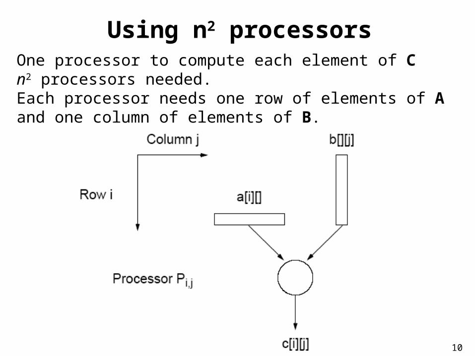
Using n2 processorsOne processor to compute each element of Cn2 processors needed.Each processor needs one row of elements of A and one column of elements of B.

11

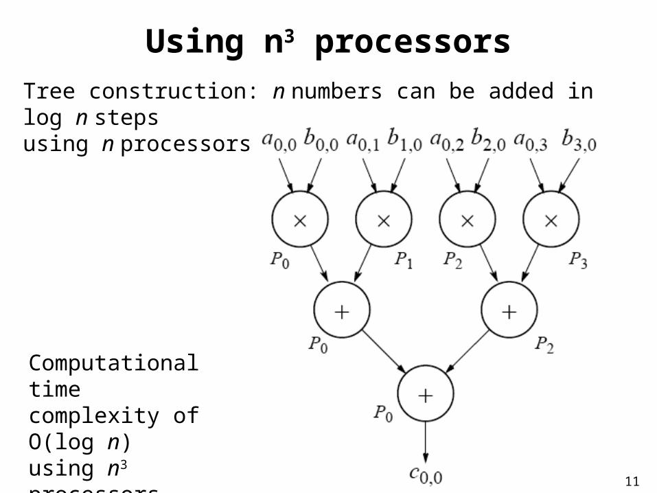
Using n3 processors

Tree construction: n numbers can be added in log n stepsusing n processors:

Computational timecomplexity of O(log n)using n3 processors.

12

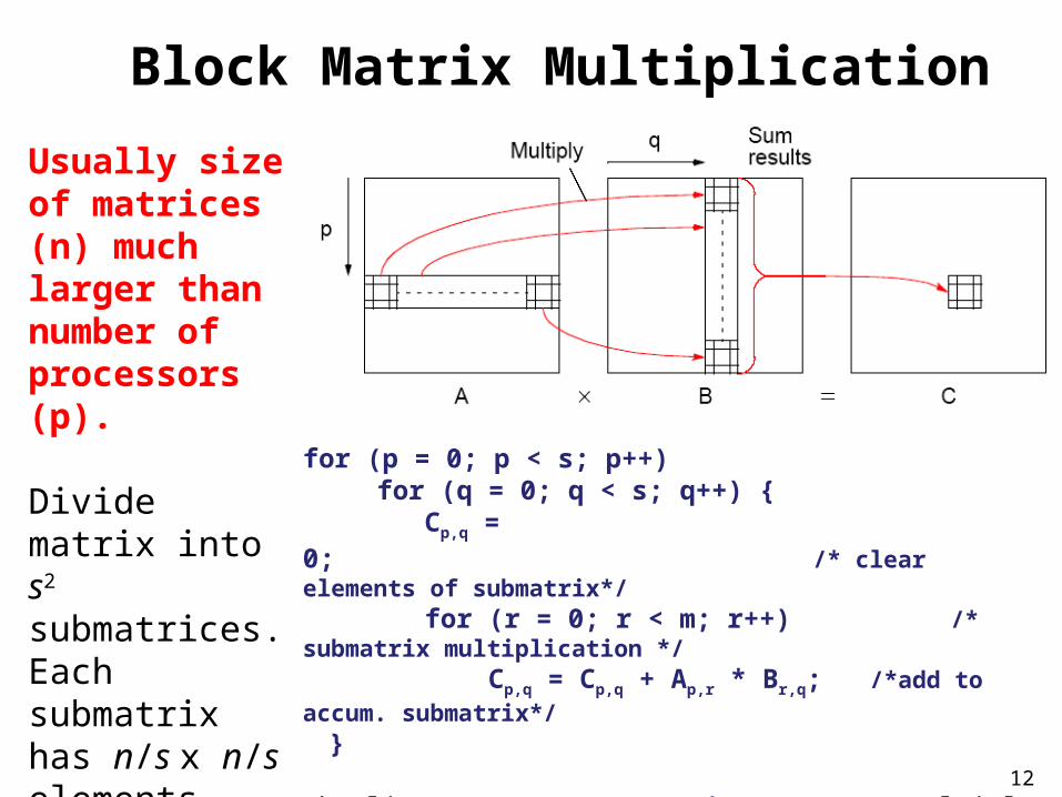
Block Matrix Multiplication

Usually size of matrices (n) much larger than number of processors (p).

Divide matrix into s2 submatrices. Each submatrix has n/s x n/s elements.

for (p = 0; p < s; p++) for (q = 0; q < s; q++) { Cp,q = 0; /* clear elements of submatrix*/

for (r = 0; r < m; r++) /* submatrix multiplication */ Cp,q = Cp,q + Ap,r * Br,q; /*add to accum. submatrix*/

}

The line: Cp,q = Cp,q + Ap,r * Br,q; means multiply submatrix Ap,r and Br,q using matrix multiplication and add to submatrix Cp,q using matrix addition.

13

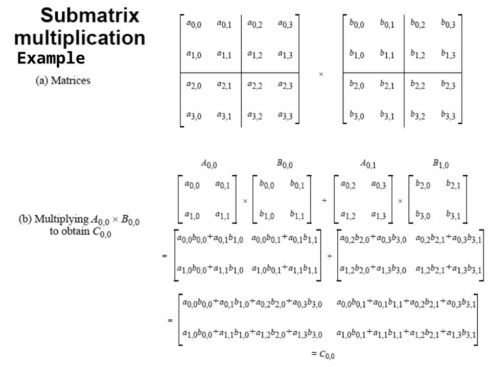
Example

14

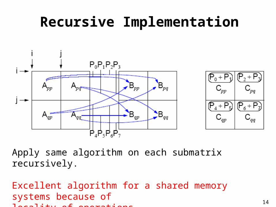
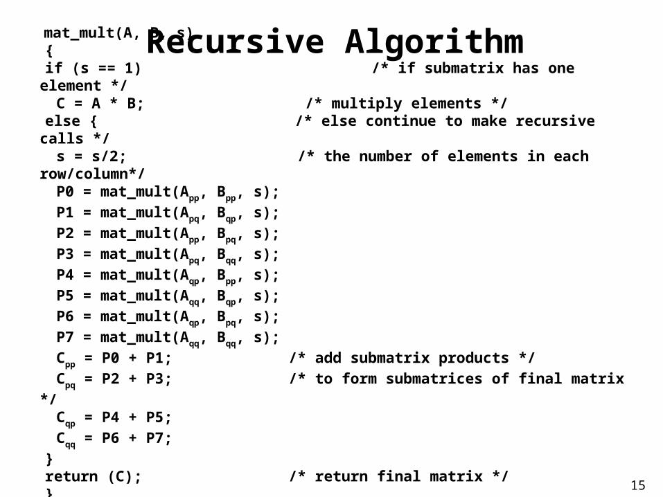
Recursive Implementation

Apply same algorithm on each submatrix recursively.

Excellent algorithm for a shared memory systems because oflocality of operations.

15

Recursive Algorithmmat_mult(A, B, s){if (s == 1) /* if submatrix has one element */

C = A * B; /* multiply elements */else { /* else continue to make recursive calls */

s = s/2; /* the number of elements in each row/column*/P0 = mat_mult(App, Bpp, s);

P1 = mat_mult(Apq, Bqp, s);

P2 = mat_mult(App, Bpq, s);

P3 = mat_mult(Apq, Bqq, s);

P4 = mat_mult(Aqp, Bpp, s);

P5 = mat_mult(Aqq, Bqp, s);

P6 = mat_mult(Aqp, Bpq, s);

P7 = mat_mult(Aqq, Bqq, s);

Cpp = P0 + P1; /* add submatrix products */

Cpq = P2 + P3; /* to form submatrices of final matrix */

Cqp = P4 + P5;

Cqq = P6 + P7;

}return (C); /* return final matrix */}

16

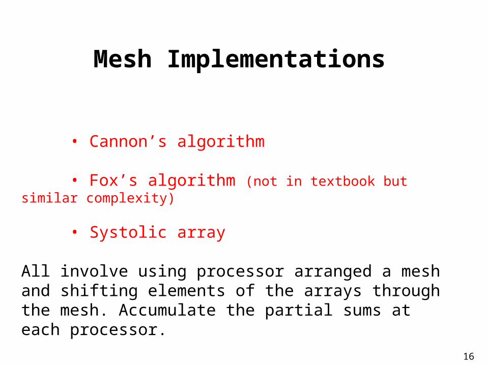
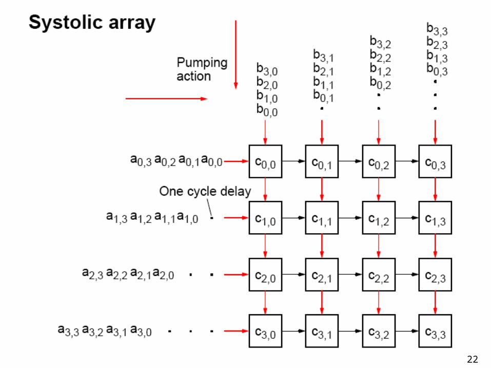
Mesh Implementations

• Cannon’s algorithm

• Fox’s algorithm (not in textbook but similar complexity)

• Systolic array

All involve using processor arranged a mesh and shifting elements of the arrays through the mesh. Accumulate the partial sums at each processor.

17

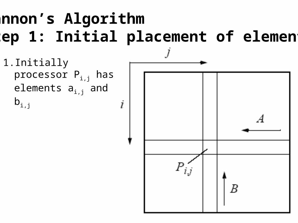
Cannon’s AlgorithmStep 1: Initial placement of elements

1. Initially processor Pi,j has elements ai,j and bi,j

18

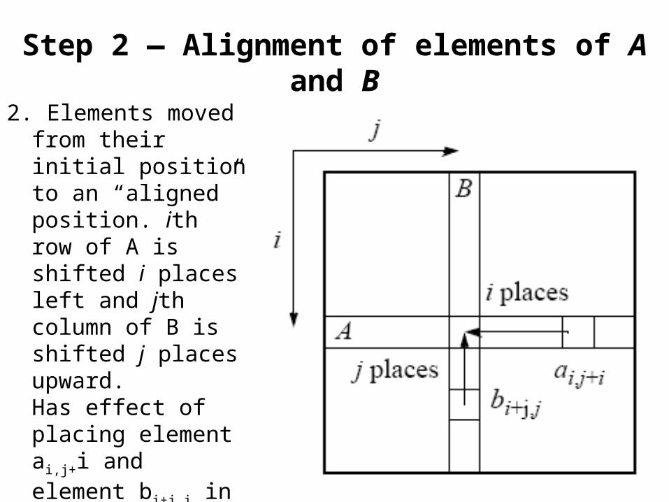
Step 2 — Alignment of elements of A and B

2. Elements moved from their initial position to an “aligned” position. ith row of A is shifted i places left and jth column of B is shifted j places upward.Has effect of placing element ai,j+i and element bi+j,j in processor Pi,j. These elements are a pair of those required in accumulation of ci,j.

19

3. Each processor, Pi,j, multiplies its elements and adds result to accumulating sum (initially sum = 0).

20

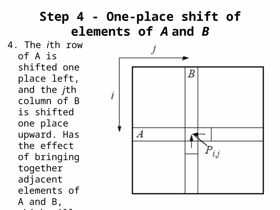
Step 4 - One-place shift of elements of A and B

4. The ith row of A is shifted one place left, and the jth column of B is shifted one place upward. Has the effect of bringing together adjacent elements of A and B, which will also be required in the accumulation.

21

Step 3 and 4 repeated until final result obtained (n - 1 shifts with n rows and n columns of elements).

22

23

24

Solving a System of Linear Equations

Objective is to find values for the unknowns, x0, x1, …, xn-1, given values for a0,0, a0,1, …, an-1,n-1, and b0, …, bn .

25

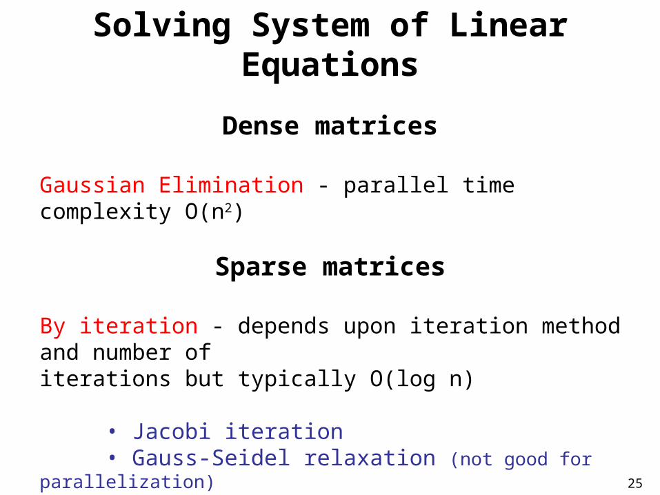
Solving System of Linear Equations

Dense matrices

Gaussian Elimination - parallel time complexity O(n2)

Sparse matrices

By iteration - depends upon iteration method and number ofiterations but typically O(log n)

• Jacobi iteration• Gauss-Seidel relaxation (not good for parallelization)

• Red-Black ordering• Multigrid

26

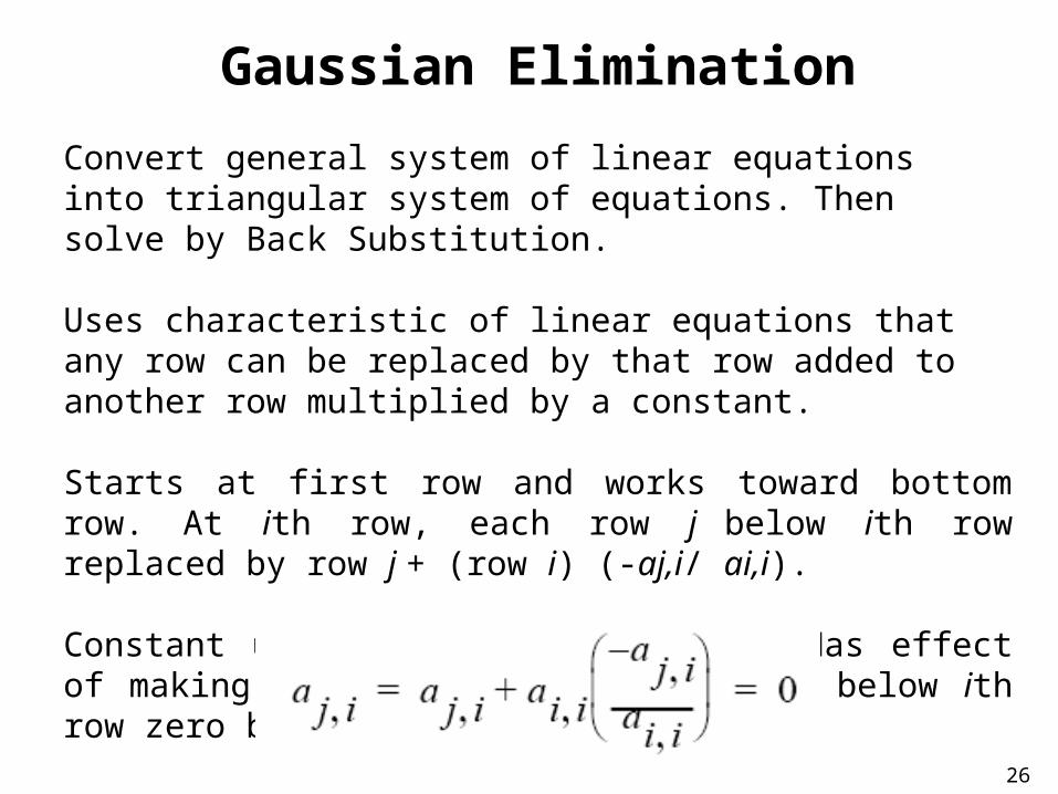
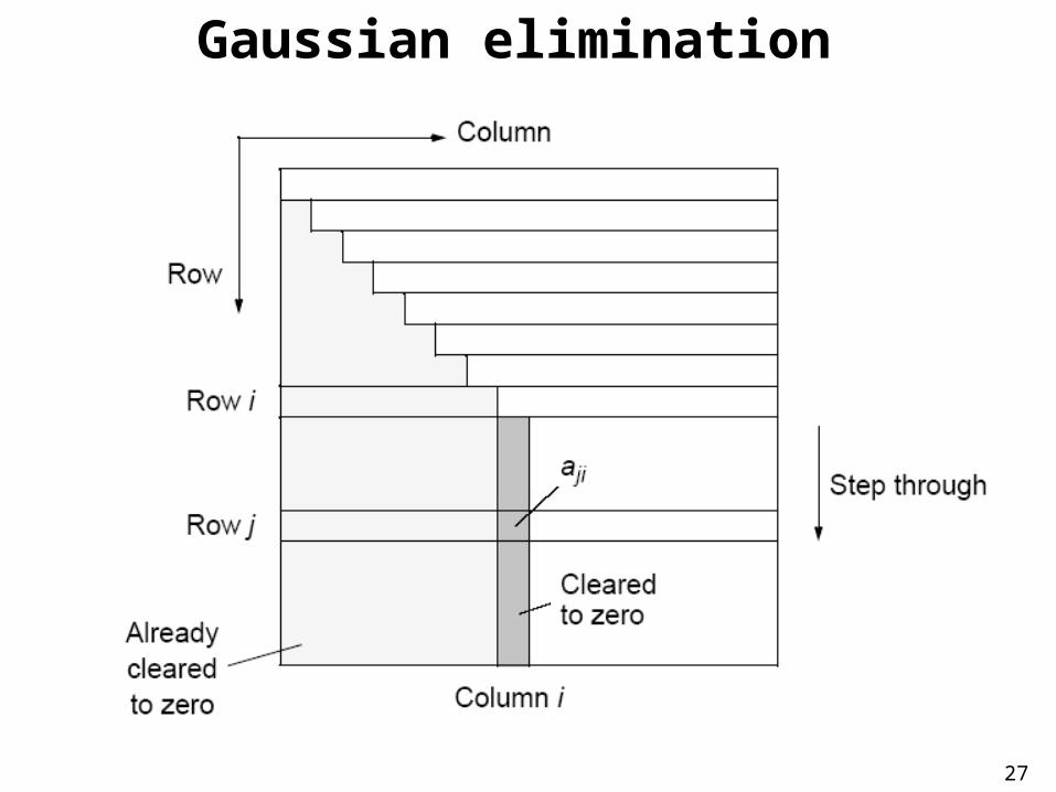
Gaussian Elimination

Convert general system of linear equations into triangular system of equations. Then solve by Back Substitution.

Uses characteristic of linear equations that any row can be replaced by that row added to another row multiplied by a constant.

Starts at first row and works toward bottom row. At ith row, each row j below ith row replaced by row j + (row i) (-aj,i/ ai,i).

Constant used for row j is -aj,i/ai,i. Has effect of making all elements in ith column below ith row zero because:

27

Gaussian elimination

28

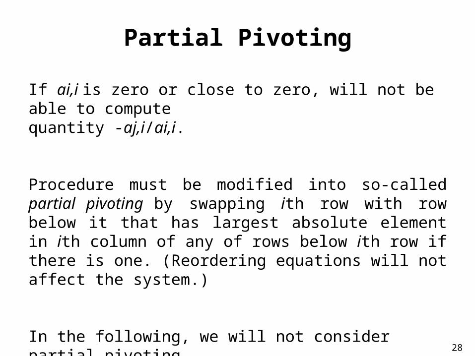
Partial Pivoting

If ai,i is zero or close to zero, will not be able to compute quantity -aj,i/ai,i.

Procedure must be modified into so-called partial pivoting by swapping ith row with row below it that has largest absolute element in ith column of any of rows below ith row if there is one. (Reordering equations will not affect the system.)

In the following, we will not consider partial pivoting.

29

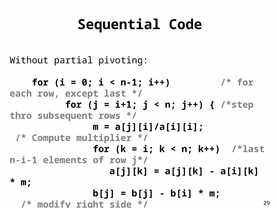
Sequential Code

Without partial pivoting:

for (i = 0; i < n-1; i++) /* for each row, except last */ for (j = i+1; j < n; j++) { /*step thro subsequent rows */ m = a[j][i]/a[i][i]; /* Compute multiplier */ for (k = i; k < n; k++) /*last n-i-1 elements of row j*/ a[j][k] = a[j][k] - a[i][k] * m; b[j] = b[j] - b[i] * m; /* modify right side */}

The time complexity is O(n3).

30

Parallel Implementation

31

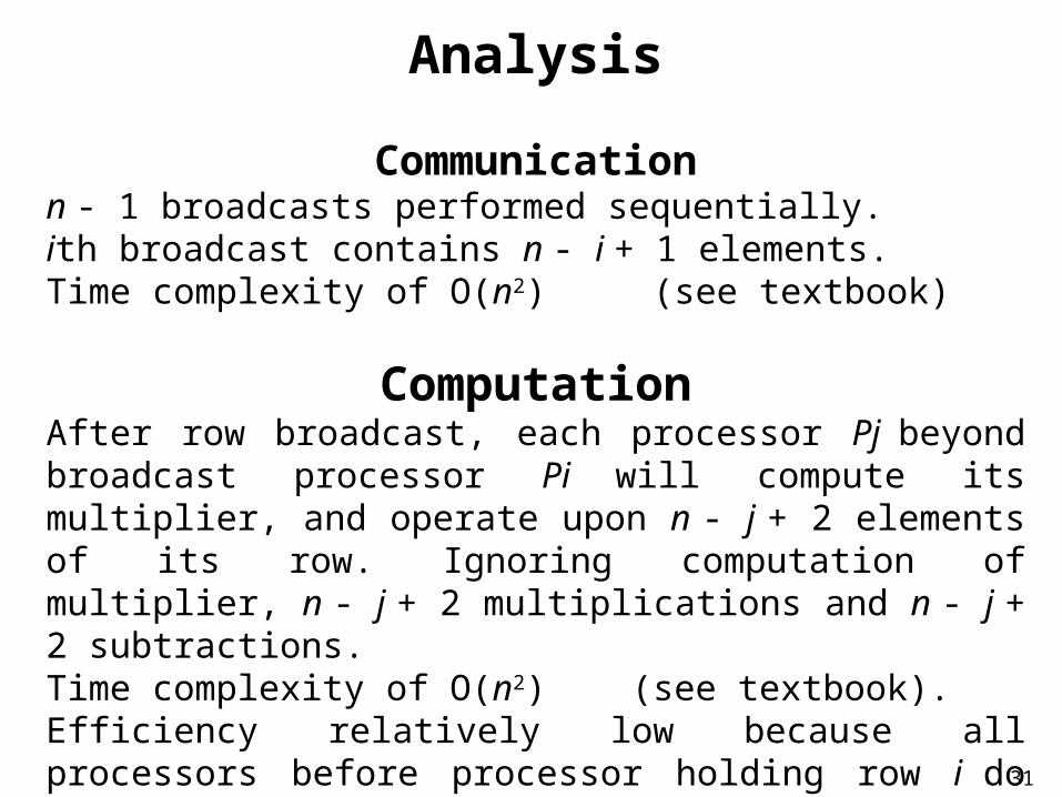
Analysis

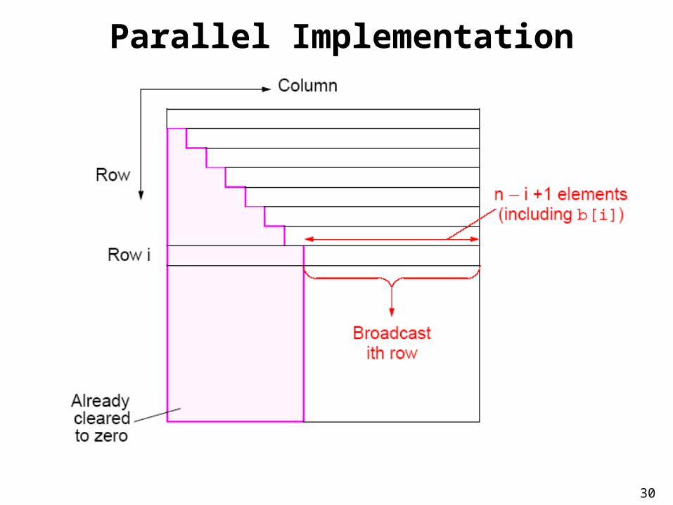
Communicationn - 1 broadcasts performed sequentially. ith broadcast contains n - i + 1 elements.Time complexity of O(n2) (see textbook)

ComputationAfter row broadcast, each processor Pj beyond broadcast processor Pi will compute its multiplier, and operate upon n - j + 2 elements of its row. Ignoring computation of multiplier, n - j + 2 multiplications and n - j + 2 subtractions.Time complexity of O(n2) (see textbook).Efficiency relatively low because all processors before processor holding row i do not participate in computation again.

32

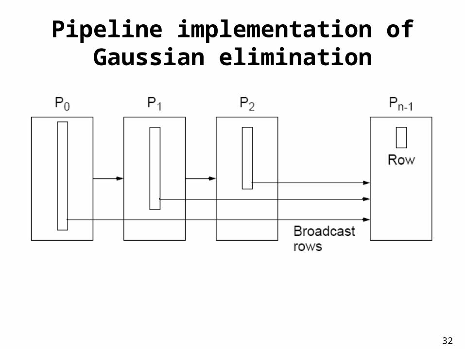
Pipeline implementation of Gaussian elimination

33

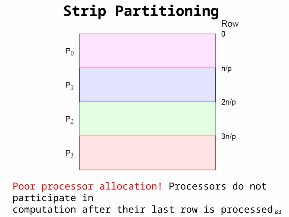
Strip Partitioning

Poor processor allocation! Processors do not participate incomputation after their last row is processed.

34

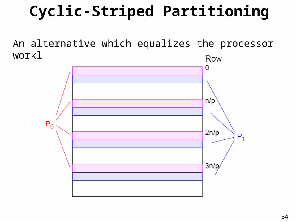
Cyclic-Striped Partitioning

An alternative which equalizes the processor workload:

35

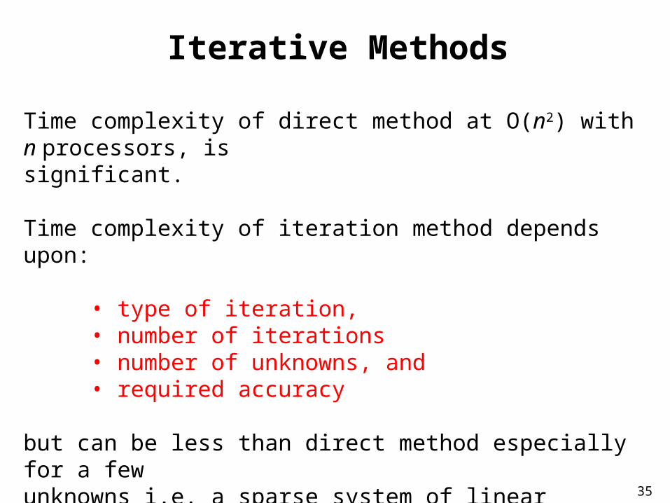
Iterative Methods

Time complexity of direct method at O(n2) with n processors, issignificant.

Time complexity of iteration method depends upon:

• type of iteration,• number of iterations• number of unknowns, and• required accuracy

but can be less than direct method especially for a fewunknowns i.e. a sparse system of linear equations.

36

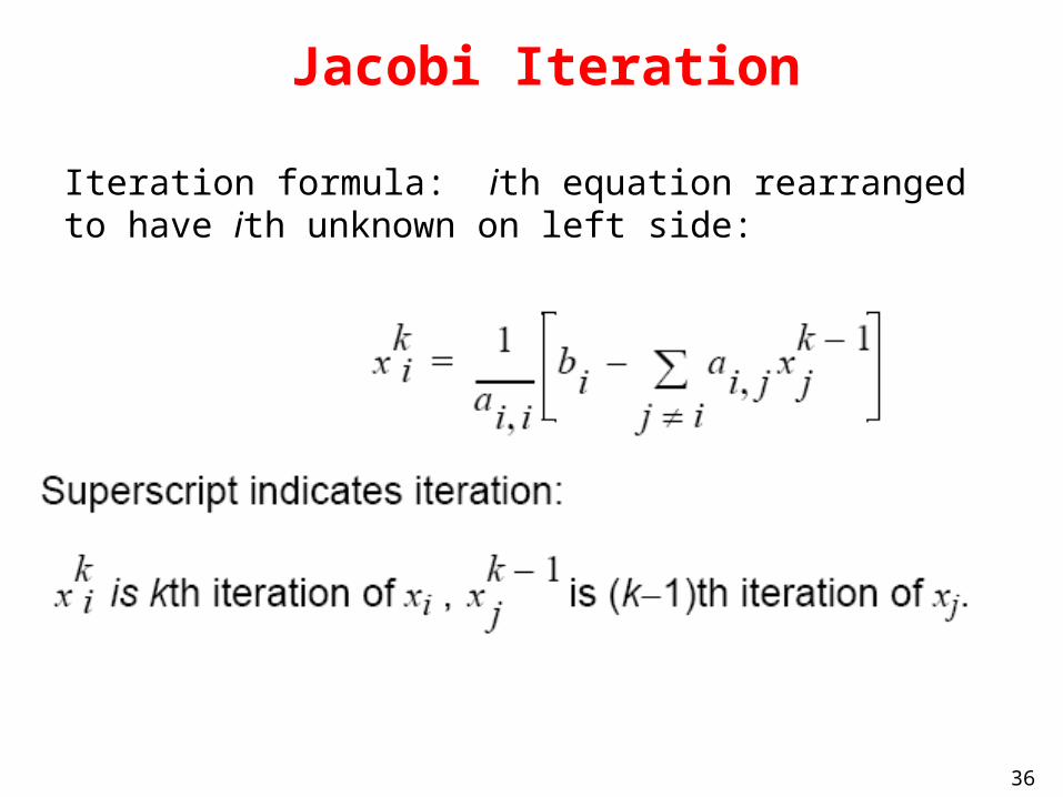
Jacobi Iteration

Iteration formula: ith equation rearranged to have ith unknown on left side:

37

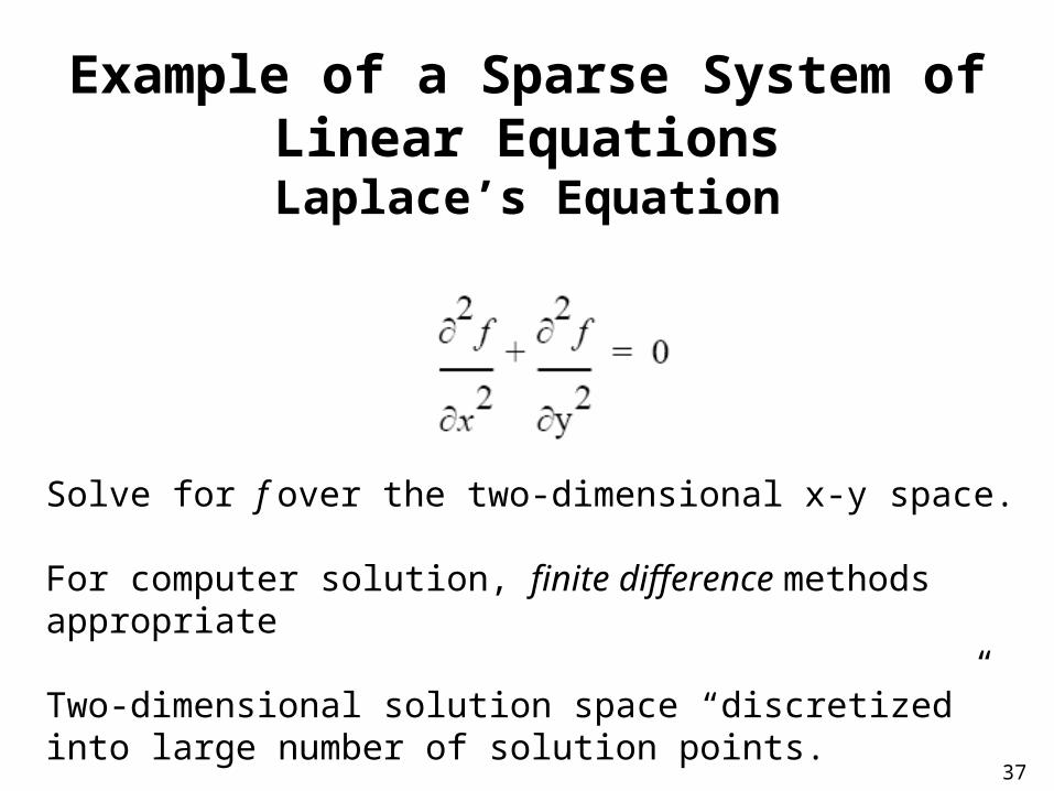
Example of a Sparse System of Linear Equations

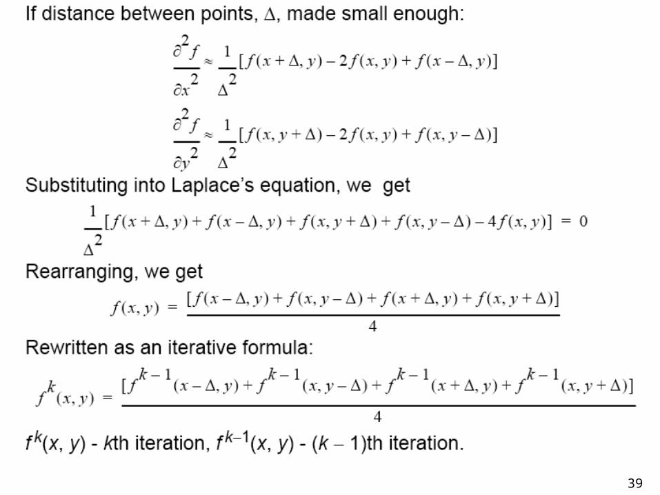
Laplace’s Equation

Solve for f over the two-dimensional x-y space.

For computer solution, finite difference methods appropriate

Two-dimensional solution space “discretized” into large number of solution points.

38

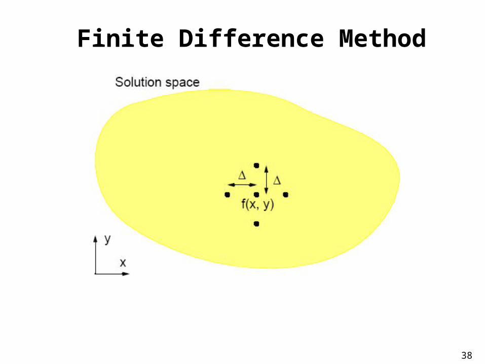
Finite Difference Method

39

40

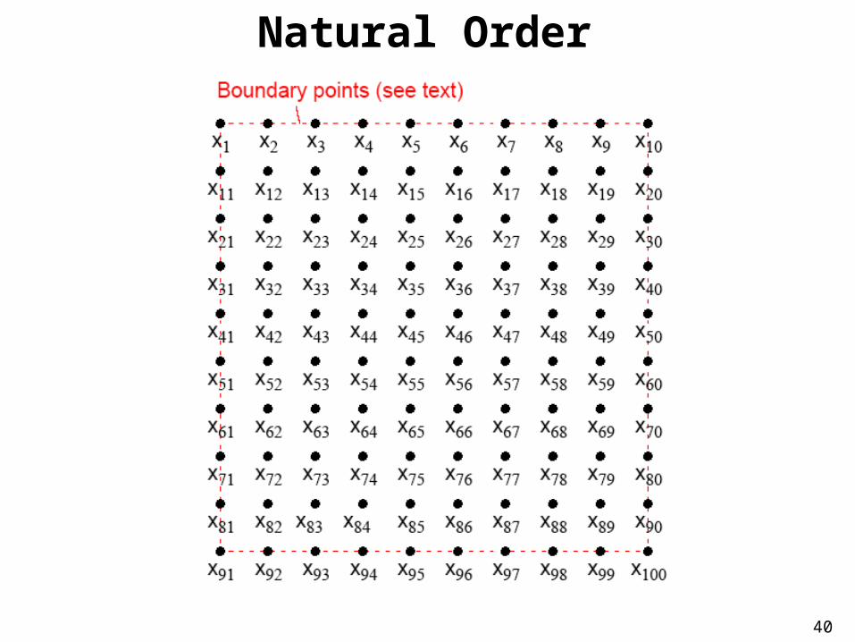
Natural Order

41

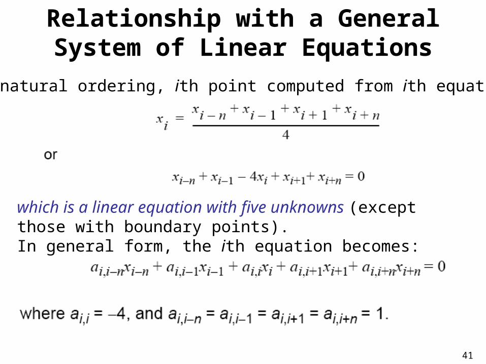
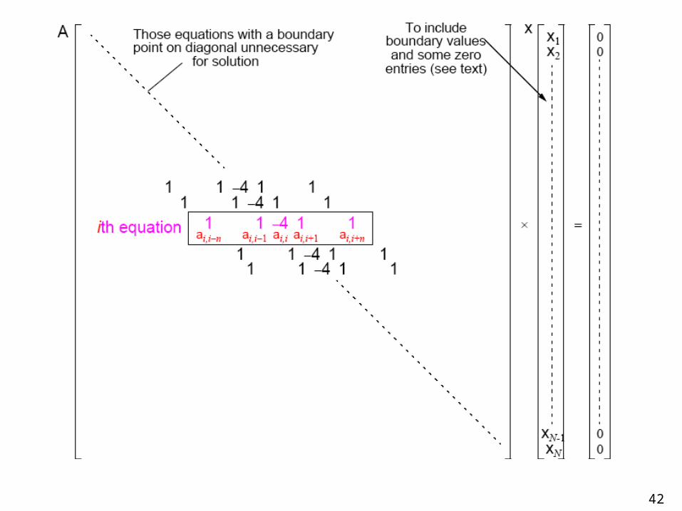
Relationship with a General System of Linear Equations

Using natural ordering, ith point computed from ith equation:

which is a linear equation with five unknowns (except those with boundary points).In general form, the ith equation becomes:

42

43

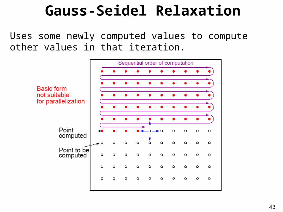
Gauss-Seidel Relaxation

Uses some newly computed values to compute other values in that iteration.

44

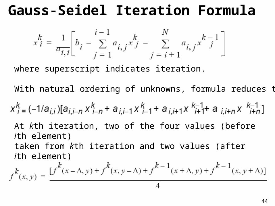
Gauss-Seidel Iteration Formula

where superscript indicates iteration.

With natural ordering of unknowns, formula reduces to

At kth iteration, two of the four values (before ith element)taken from kth iteration and two values (after ith element)taken from (k-1)th iteration. Have:

45

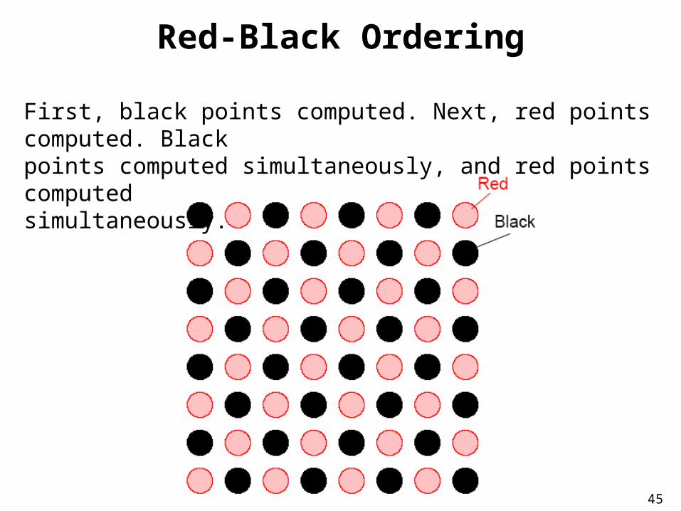
Red-Black Ordering

First, black points computed. Next, red points computed. Blackpoints computed simultaneously, and red points computedsimultaneously.

46

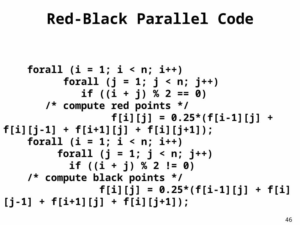
Red-Black Parallel Code

forall (i = 1; i < n; i++) forall (j = 1; j < n; j++) if ((i + j) % 2 == 0) /* compute red points */ f[i][j] = 0.25*(f[i-1][j] + f[i][j-1] + f[i+1][j] + f[i][j+1]); forall (i = 1; i < n; i++) forall (j = 1; j < n; j++) if ((i + j) % 2 != 0) /* compute black points */ f[i][j] = 0.25*(f[i-1][j] + f[i][j-1] + f[i+1][j] + f[i][j+1]);

47

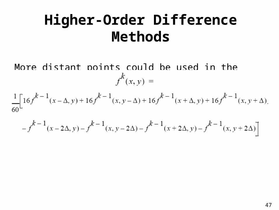
Higher-Order Difference Methods

More distant points could be used in the computation. The following update formula:

48

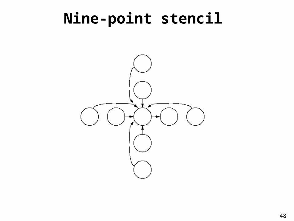
Nine-point stencil

49

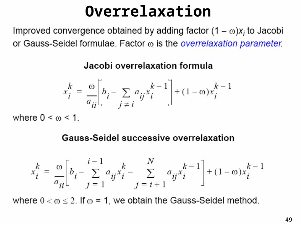
Overrelaxation

50

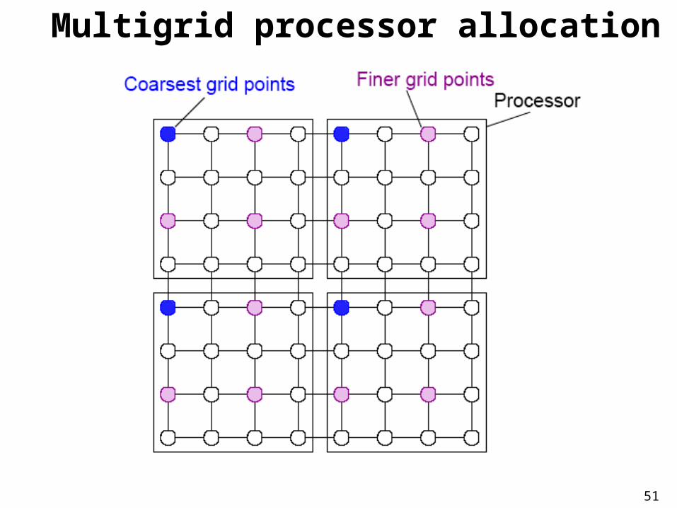
Multigrid Method

First, a coarse grid of points used. With these points, iteration process will start to converge quickly.

At some stage, number of points increased to include points of coarse grid and extra points between points of coarse grid. Initial values of extra points found by interpolation. Computation continues with this finer grid.

Grid can be made finer and finer as computation proceeds, or computation can alternate between fine and coarse grids.

Coarser grids take into account distant effects more quickly and provide a good starting point for the next finer grid.

51

Multigrid processor allocation

52

(Semi) Asynchronous Iteration

As noted early, synchronizing on every iteration will cause significant overhead - best if one can is to synchronize after anumber of iterations.