1

Particle Filters forPositioning, Navigation and Tracking

Fredrik Gustafsson, Fredrik Gunnarsson, Niclas Bergman, Urban Forssell,Jonas Jansson, Rickard Karlsson, Per-Johan Nordlund

Final version for IEEE Transactions on Signal Processing.Special issue on Monte Carlo methods for statistical signal processing.

1

Abstract— A framework for positioning, navigation andtracking problems using particle filters (sequential MonteCarlo methods) is developed. It consists of a class of mo-tion models and a general non-linear measurement equa-tion in position. A general algorithm is presented, whichis parsimonious with the particle dimension. It is basedon marginalization, enabling a Kalman filter to estimateall position derivatives, and the particle filter becomeslow-dimensional. This is of utmost importance for high-performance real-time applications.

Automotive and airborne applications illustrate numeri-cally the advantage over classical Kalman filter based algo-rithms. Here the use of non-linear models and non-Gaussiannoise is the main explanation for the improvement in accu-racy.

More specifically, we describe how the technique of mapmatching is used to match an aircraft’s elevation profile to adigital elevation map, and a car’s horizontal driven path toa street map. In both cases, real-time implementations areavailable, and tests have shown that the accuracy in bothcases is comparable to satellite navigation (as GPS), butwith higher integrity. Based on simulations, we also arguehow the particle filter can be used for positioning based oncellular phone measurements, for integrated navigation inaircraft, and for target tracking in aircraft and cars. Fi-nally, the particle filter enables a promising solution to thecombined task of navigation and tracking, with possible ap-plication to airborne hunting and collision avoidance systemsin cars.

I. Introduction

Recursive implementations of Monte Carlo based statis-tical signal processing [19] are known as particle filters, see[13], [14]. The research has since the paper [21] steadilyintensified, see the recent first article collection [13]. Theparticle filters may be a serious alternative for real-time ap-plications classically approached by model-based Kalmanfilter techniques [29], [24]. The more non-linear model, orthe more non-Gaussian noise, the more potential particlefilters have, especially in applications where computationalpower is rather cheap and the sampling rate is moderate.

1Fredrik Gustafsson, Fredrik Gunnarsson, Jonas Jansson, RickardKarlsson and Per-Johan Nordlund are with the Department of Elec-trical Engineering, Linkoping University, 58183 Linkoping, Sweden(email: {fredrik,fred,jansson,rickard,perno}@isy.liu.se).Fredrik Gunnarsson is also with Ericsson Radio, Sweden.Urban Forssell is with NIRA Dynamics AB, 58330 Linkoping, Swe-den. (urban.forssell@niradynamics.se).Niclas Bergman is with SaabTech Systems, 17588 Jarfalla, Sweden.(email: ncbe@systems.saab.se).Jonas Jansson is also with Volvo Car Corporation, Sweden.Rickard Karlsson is also with Saab Dynamics, Sweden.Per-Johan Nordlund is also with Saab Gripen, Sweden.

The paper describes a general framework for a numberof applications, where we have implemented the particlefilter. The problem areas are• Positioning, where one’s own position is to be estimated.This is a filtering problem rather than a static estimationproblem, when an inertial navigation system is used to pro-vide measurements of movement.• Navigation, where besides the position also velocity, at-titude and heading, acceleration and angular rates are in-cluded in the filtering problem.• Target tracking, where another object’s position is to beestimated based on measurements of relative range and an-gles to one’s own position.Another related application fitting this framework, not ex-plicitly included here, is robot localization, see for instance[43], [44]. The problems listed above are related in thatthey can be described by quite similar state space models,where the state vector contains the position and deriva-tives of the position. Traditional methods are based onlinearized models and Gaussian noise approximations sothat the Kalman filter can be applied [1]. Research is fo-cused on how different state coordinates or multiple mod-els can be used to limit the approximations. In contrastto this, the particle filter approximates the optimal solu-tion numerically based on a physical model, rather thanapplying an optimal filter to an approximate model. Awell-known problem with the particle filter is that its per-formance degrades quickly when the dimension of the statedimension increases. A key theoretical contribution here isto apply marginalization techniques [36], adopted and ex-tended from [12], leading to that the Kalman filter can beused to estimate (or eliminate) all position derivatives, andthe particle filter is applied to the part of the state vectorcontaining only the position. Thus, the particle filter di-mension is only 2 or 3, depending on the application, andthis is the main step to get real-time high-performance al-gorithms.

The applications we will describe are:• Car positioning by map matching. A digital road mapis used to constrain the possible positions, where a dead-reckoning of wheel speeds is the main external input to thealgorithm. By matching the driven path to a road map, avague initial position (order of km’s) can be improved toa meter accuracy. This principle can be used as a supple-ment to, or even replacement to, GPS (global positioningsystem).

2

• Car positioning by Radio Frequency (RF) measurements.The digital road map above can be replaced by, or supple-mented by, measurements from a terrestrial wireless com-munications system. For hand-over (to transfer a connec-tion from one base station to another) operation, the mo-bile stations (MS) monitor the received signal powers froma multitude of base stations, and report regularly to thenetwork. These measurements provide a power map whichcan be used in a similar manner as above. Mobile stationsin a near future will moreover provide the possibility ofmonitoring the traveled distance of the radio signals froma number of base stations [16]. Such measurements can alsobe utilized in the same manner as with the power measure-ments.• Aircraft positioning by map matching or terrain nav-igation. A Geographical information system contains,among other information, terrain elevation. The aircraftis equipped with sensors such that the terrain elevationcan be measured. By map matching, the position can bededucted [5].• Integrated navigation. The aircraft’s Inertial NavigationSystem (INS) uses dead-reckoning to compute navigationand flight data, i.e. position, velocity, attitude and head-ing. The INS is regarded as the main sensor for navigationand flight data due to being autonomous and having highreliability [10]. However, small offsets cause drift and itsoutput has to be stabilized. Here, terrain navigation isused today.• Target tracking. A classical problem in signal processingliterature is target tracking, where an IR sensor measuresrelative angle, or a radar measures relative angle, range andpossibly range rate, to the object [4]. For the case of bear-ings only measuring IR sensor, either the state dynamicsor measurement equation is very non-linear depending onthe choice of state coordinates, so here the particle filter isparticularly promising.• Combined navigation and tracking. Because the targettracking measurements are relative to one’s own platform,positioning is an important sub-problem. Since the sensorintroduces a cross-coupling between the problems, a unifiedtreatment is tempting.• Car collision avoidance is very similar to the target track-ing problem, here we are interested in predicting the owncar’s and other objects’ future position, see [40]. Based onthe prediction, collision avoidance actions such as warn-ing, braking and steering are undertaken when a collisionis likely to happen. In order to have enough time to warnthe driver the prediction horizon needs to be quite long.Therefore, utilizing knowledge about road geometry andinfrastructure becomes important. One way to improvethe prediction of possible maneuvers, is to use informationin a digital map. Thus, this is a specific project includingall aspects of the problems listed above.

The outline is as follows. We will start with a generalframework of models covering all of our applications in Sec-tion II. Then, a general algorithm is presented covering allapplications, where special attention is paid on practicalproblems as divergence test, initialization and real-time re-

quirements. Each application in the list above is devotedits own section, and conclusions and open questions of gen-eral interest are discussed in VIII.

II. Models

Central for all navigation and tracking applications is themotion model to which various kind of model based filterscan be applied. Models which are linear in the state dy-namics and non-linear in the measurements are considered:

xt+1 = Axt +Buut +Bfft, (1a)yt = h(xt) + et. (1b)

Here xt is the state vector, ut measured inputs, ft unmea-sured forces or faults, yt the measurements and et mea-surement error. We assume independent distributions forft, et and x0, with known probability densities pet , pft andpx0 , respectively, not necessarily Gaussian. Motion mod-els (1a) are further discussed in Section II-A. These areto a large extent similar in all applications, and standardin the literature. The model (1) takes only movementsinto account, and we do not attempt to model for instancemechanical dynamics in the platform. That is, (1) haveno model parameters. The difference between the applica-tions mainly lies in the availability of measurements. Sec-tion II-B provides an extensive list of possible measurementequations (1b).

A. Motion Models

The signals of primary interest in navigation and track-ing applications are related to position, velocity and ac-celeration as summarized in Table I. Newton’s law relates

Object Position Velocity AccelerationOwn p(1) v(1) a(1), δa(1) acc. biasOther p(2) v(2) -

TABLE I

Interesting signals in navigation and tracking applications.

Index (1) and (2) indicates signals related to one’s own and

another platform respectively. All quantities can belong

to either one, two or three-dimensional spaces, depending on

the application.

known and unknown external forces on the platforms toacceleration. From the differential equations pt = vt andvt = at, we obtain relations like pt = p0 + v0t if velocity isassumed constant and pt = p0 +v0t+a0t

2/2 if accelerationis assumed constant. If we here plug in the sample periodTs, we get a discrete time model for motion between twoconsecutive measurements as will be frequently used in thesequel.

Depending on whether the signals are measurable or not,they may be components of either the state vector xt orthe input signal ut. The ambition here is to discuss mod-els through which the applications are naturally related.

3

In specific applications, however, other parameterizationsmight provide better understanding of design variables andalgorithm tuning.

In positioning and navigation applications the signals re-lated to the own platform are of interest. If the velocity v(1)

t

is assumed measurable (and thus part of the input signal),the state dynamics can be modeled as

p(1)t+1 = p

(1)t︸︷︷︸xt

+Tsv(1)t︸ ︷︷ ︸

Buut

+Tsf(1)t︸ ︷︷ ︸

Bfft

. (2a)

In several navigation applications, such as airborne, mea-surements of the acceleration are used instead of velocity.These are typically biased, and the true acceleration canbe expressed as

a(1)true,t = a

(1)t + δa

(1)t ,

where a(1)t is the measured acceleration and δa

(1)t is the

bias. The position is extracted by dead-reckoning of themeasured acceleration, and therefore the presence of accel-eration bias is critical. The natural thing to do is to includethe bias in the state vector, and the measured accelerationin the input signal. The resulting motion model is

p(1)t+1

v(1)t+1

δa(1)t+1

=

I Ts · I T 2s /2 · I

0 I Ts · I0 0 I

︸ ︷︷ ︸

A(1)

p(1)t

v(1)t

δa(1)t

+

T 2s /2 · ITs · I

0

︸ ︷︷ ︸

B(1)u

a(1)t +

T 3s /6 · IT 2s /2 · ITs · I

︸ ︷︷ ︸

B(1)f

f(1)t . (2b)

Analogously, a bias in any other measured signal (e.g. abias in the velocity in Equation (2a)) can be considered byincorporating it in the state equation.

So far, the focus has been on the own platform. In asimple model of the movements of the other platform, theassumption is that its velocity v(2) is subject to an unknownacceleration. This yields

(p

(2)t+1

v(2)t+1

)=(I Ts · I0 I

)︸ ︷︷ ︸

A(2)

(p

(2)t

v(2)t

)+(T 2s /2 · ITs · I

)︸ ︷︷ ︸

B(2)f

f(2)t . (2c)

In the target tracking literature, a popular choice of motionmodel is given by the “coordinated turn”-model [4].

When considering tracking of another platform, whilemoving the own platform, joint navigation and targettracking can be employed. Essentially, the total motion

model comprises the motion models (2b) and (2c):p

(1)t+1

v(1)t+1

δa(1)t+1

p(2)t+1

v(2)t+1

=(A(1) 0

0 A(2)

)p

(1)t

v(1)t

δa(1)t

p(2)t

v(2)t

+(B

(1)u

0

)a

(1)t +

(B

(1)f 00 B

(2)f

)(f

(1)t

f(2)t

). (2d)

B. Measurement Equations

The main difference between the considered applicationsis the measurements available. Basically, the measure-ments are related to the positions of one’s own platformp(1) and to the other object p(2). Therefore, the measure-ment equations can be categorized as depending on p(1)

only, or depending on both p(1) and p(2):

y(1)t = h(1)(p(1)

t ) + e(1)t (3a)

y(2)t = h(2)(p(1)

t , p(2)t ) + e

(2)t , (3b)

where the measurement noise contributions e(1)t and e

(2)t

are characterized by their distributions. If not explicitlymentioned, a Gaussian distribution is used.

In the studied applications, measurements from at leastone of the categories above are available. It is important tonote, that any combination of the sensors is possible. Thepresented applications are just a few examples.

B.1 Measurements of Relative Distance

As always, any position has to be related to a coordinatesystem and a reference position. Several types of sensors(e.g. GPS, RF) basically measure the distance relative tothat reference point. One possibility is distance measure-ments of the own position relative to points of known po-sitions pi, i = 1, . . . ,M , which yields M measurementequations with

h(1)a,i(p

(1)t ) =

∣∣∣pi − p(1)t

∣∣∣ , i = 1, . . . ,M. (3c)

This is also applicable when the position of another objectis related to one’s own position (e.g. radar, sonar, ultra-sound):

h(2)b (p(1)

t , p(2)t ) =

∣∣∣p(2)t − p

(1)t

∣∣∣ . (3d)

Some sensors do not measure the relative distance explic-itly, but rather a quantity related to the same. One exam-ple is sensors that measure the received radio signal powertransmitted from a known position pi. This received powertypically decays as ∼ K1/|pi − p(1)

t |α, α ∈ [2, 5], where K1

and α depend on the radio environment, antenna character-istics, terrain etc. In a logarithmic scale, the measurementsare given by

h(1)c,i (p

(1)t ) = K − α log10

∣∣∣pi − p(1)t

∣∣∣ , i = 1, . . . ,M, (3e)

4

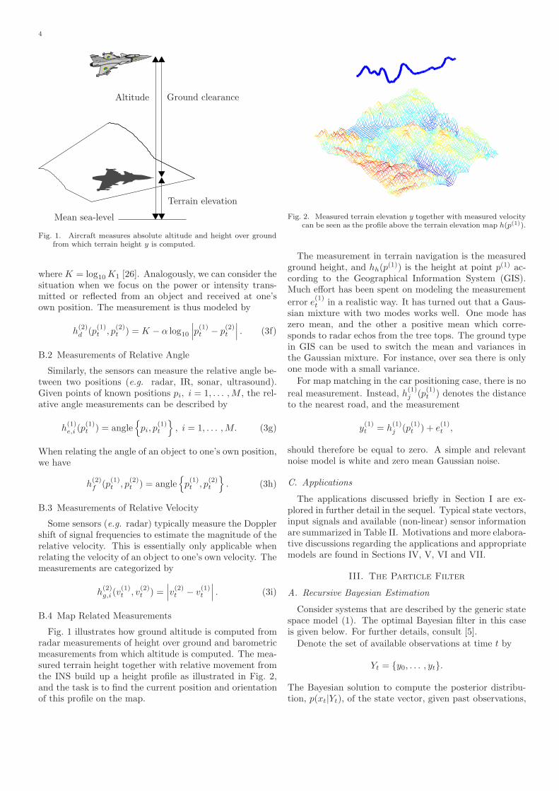
Altitude Ground clearance

Mean sea-level

Terrain elevation

Fig. 1. Aircraft measures absolute altitude and height over groundfrom which terrain height y is computed.

where K = log10K1 [26]. Analogously, we can consider thesituation when we focus on the power or intensity trans-mitted or reflected from an object and received at one’sown position. The measurement is thus modeled by

h(2)d (p(1)

t , p(2)t ) = K − α log10

∣∣∣p(1)t − p

(2)t

∣∣∣ . (3f)

B.2 Measurements of Relative Angle

Similarly, the sensors can measure the relative angle be-tween two positions (e.g. radar, IR, sonar, ultrasound).Given points of known positions pi, i = 1, . . . ,M , the rel-ative angle measurements can be described by

h(1)e,i (p

(1)t ) = angle

{pi, p

(1)t

}, i = 1, . . . ,M. (3g)

When relating the angle of an object to one’s own position,we have

h(2)f (p(1)

t , p(2)t ) = angle

{p

(1)t , p

(2)t

}. (3h)

B.3 Measurements of Relative Velocity

Some sensors (e.g. radar) typically measure the Dopplershift of signal frequencies to estimate the magnitude of therelative velocity. This is essentially only applicable whenrelating the velocity of an object to one’s own velocity. Themeasurements are categorized by

h(2)g,i (v

(1)t , v

(2)t ) =

∣∣∣v(2)t − v

(1)t

∣∣∣ . (3i)

B.4 Map Related Measurements

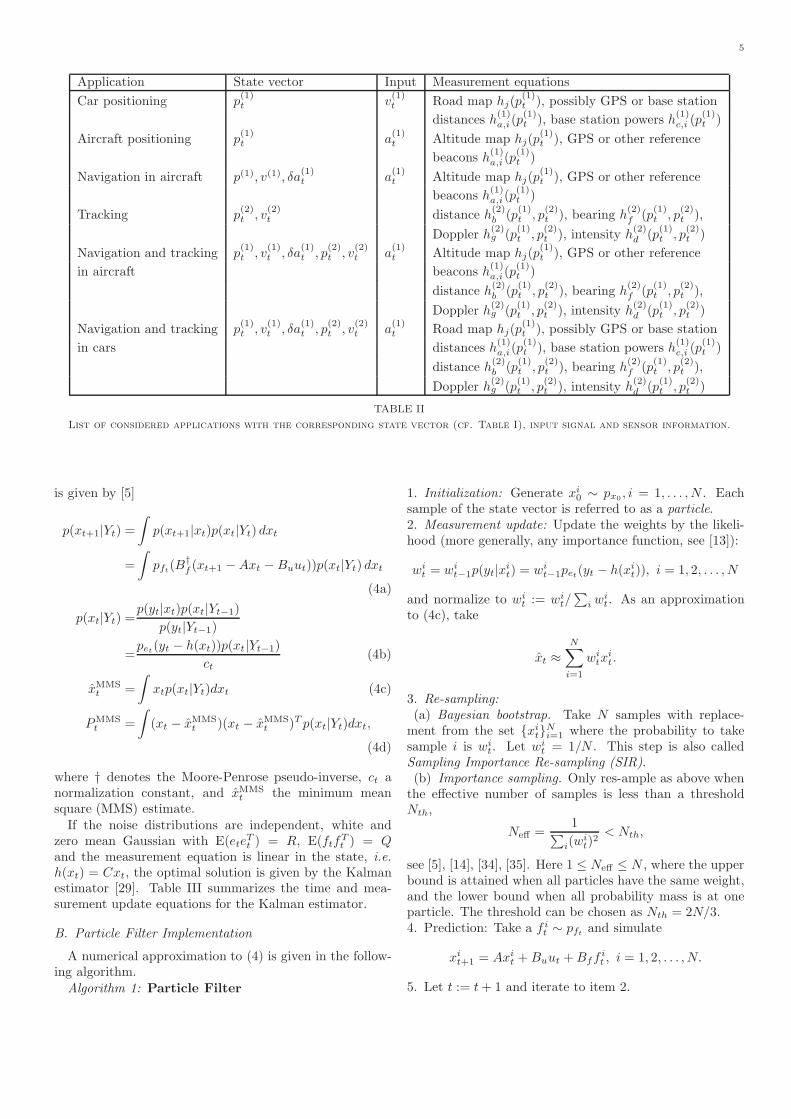
Fig. 1 illustrates how ground altitude is computed fromradar measurements of height over ground and barometricmeasurements from which altitude is computed. The mea-sured terrain height together with relative movement fromthe INS build up a height profile as illustrated in Fig. 2,and the task is to find the current position and orientationof this profile on the map.

Fig. 2. Measured terrain elevation y together with measured velocitycan be seen as the profile above the terrain elevation map h(p(1)).

The measurement in terrain navigation is the measuredground height, and hh(p(1)) is the height at point p(1) ac-cording to the Geographical Information System (GIS).Much effort has been spent on modeling the measurementerror e(1)

t in a realistic way. It has turned out that a Gaus-sian mixture with two modes works well. One mode haszero mean, and the other a positive mean which corre-sponds to radar echos from the tree tops. The ground typein GIS can be used to switch the mean and variances inthe Gaussian mixture. For instance, over sea there is onlyone mode with a small variance.

For map matching in the car positioning case, there is noreal measurement. Instead, h(1)

j (p(1)t ) denotes the distance

to the nearest road, and the measurement

y(1)t = h

(1)j (p(1)

t ) + e(1)t ,

should therefore be equal to zero. A simple and relevantnoise model is white and zero mean Gaussian noise.

C. Applications

The applications discussed briefly in Section I are ex-plored in further detail in the sequel. Typical state vectors,input signals and available (non-linear) sensor informationare summarized in Table II. Motivations and more elabora-tive discussions regarding the applications and appropriatemodels are found in Sections IV, V, VI and VII.

III. The Particle Filter

A. Recursive Bayesian Estimation

Consider systems that are described by the generic statespace model (1). The optimal Bayesian filter in this caseis given below. For further details, consult [5].

Denote the set of available observations at time t by

Yt = {y0, . . . , yt}.

The Bayesian solution to compute the posterior distribu-tion, p(xt|Yt), of the state vector, given past observations,

5

Application State vector Input Measurement equationsCar positioning p

(1)t v

(1)t Road map hj(p

(1)t ), possibly GPS or base station

distances h(1)a,i(p

(1)t ), base station powers h(1)

c,i (p(1)t )

Aircraft positioning p(1)t a

(1)t Altitude map hj(p

(1)t ), GPS or other reference

beacons h(1)a,i(p

(1)t )

Navigation in aircraft p(1), v(1), δa(1)t a

(1)t Altitude map hj(p

(1)t ), GPS or other reference

beacons h(1)a,i(p

(1)t )

Tracking p(2)t , v

(2)t distance h(2)

b (p(1)t , p

(2)t ), bearing h(2)

f (p(1)t , p

(2)t ),

Doppler h(2)g (p(1)

t , p(2)t ), intensity h(2)

d (p(1)t , p

(2)t )

Navigation and tracking p(1)t , v

(1)t , δa

(1)t , p

(2)t , v

(2)t a

(1)t Altitude map hj(p

(1)t ), GPS or other reference

in aircraft beacons h(1)a,i(p

(1)t )

distance h(2)b (p(1)

t , p(2)t ), bearing h(2)

f (p(1)t , p

(2)t ),

Doppler h(2)g (p(1)

t , p(2)t ), intensity h(2)

d (p(1)t , p

(2)t )

Navigation and tracking p(1)t , v

(1)t , δa

(1)t , p

(2)t , v

(2)t a

(1)t Road map hj(p

(1)t ), possibly GPS or base station

in cars distances h(1)a,i(p

(1)t ), base station powers h(1)

c,i (p(1)t )

distance h(2)b (p(1)

t , p(2)t ), bearing h(2)

f (p(1)t , p

(2)t ),

Doppler h(2)g (p(1)

t , p(2)t ), intensity h(2)

d (p(1)t , p

(2)t )

TABLE II

List of considered applications with the corresponding state vector (cf. Table I), input signal and sensor information.

is given by [5]

p(xt+1|Yt) =∫p(xt+1|xt)p(xt|Yt) dxt

=∫pft(B

†f (xt+1 −Axt −Buut))p(xt|Yt) dxt

(4a)

p(xt|Yt) =p(yt|xt)p(xt|Yt−1)

p(yt|Yt−1)

=pet(yt − h(xt))p(xt|Yt−1)

ct(4b)

xMMSt =

∫xtp(xt|Yt)dxt (4c)

PMMSt =

∫(xt − xMMS

t )(xt − xMMSt )T p(xt|Yt)dxt,

(4d)

where † denotes the Moore-Penrose pseudo-inverse, ct anormalization constant, and xMMS

t the minimum meansquare (MMS) estimate.

If the noise distributions are independent, white andzero mean Gaussian with E(eteTt ) = R, E(ftfTt ) = Qand the measurement equation is linear in the state, i.e.h(xt) = Cxt, the optimal solution is given by the Kalmanestimator [29]. Table III summarizes the time and mea-surement update equations for the Kalman estimator.

B. Particle Filter Implementation

A numerical approximation to (4) is given in the follow-ing algorithm.

Algorithm 1: Particle Filter

1. Initialization: Generate xi0 ∼ px0 , i = 1, . . . , N . Eachsample of the state vector is referred to as a particle.2. Measurement update: Update the weights by the likeli-hood (more generally, any importance function, see [13]):

wit = wit−1p(yt|xit) = wit−1pet(yt − h(xit)), i = 1, 2, . . . , N

and normalize to wit := wit/∑i w

it. As an approximation

to (4c), take

xt ≈N∑i=1

witxit.

3. Re-sampling:(a) Bayesian bootstrap. Take N samples with replace-

ment from the set {xit}Ni=1 where the probability to takesample i is wit. Let wit = 1/N . This step is also calledSampling Importance Re-sampling (SIR).(b) Importance sampling. Only res-ample as above when

the effective number of samples is less than a thresholdNth,

Neff =1∑

i(wit)2

< Nth,

see [5], [14], [34], [35]. Here 1 ≤ Neff ≤ N , where the upperbound is attained when all particles have the same weight,and the lower bound when all probability mass is at oneparticle. The threshold can be chosen as Nth = 2N/3.4. Prediction: Take a f it ∼ pft and simulate

xit+1 = Axit +Buut +Bffit , i = 1, 2, . . . , N.

5. Let t := t+ 1 and iterate to item 2.

6

The key point with re-sampling is to prevent high concen-tration of probability mass at a few particles. Withoutthis step, some wit will converge to 1 and the filter wouldbrake down to a pure simulation. The re-sampling can beefficiently implemented using a classical algorithm for sam-pling N ordered independent identically distributed vari-ables [5], [39].

It can be shown analytically [11], that under some con-ditions the estimation error is bounded by gt/N . The func-tion gt grows with time, but does not depend on the dimen-sion of the state space. That is, in theory we can expectthe same good performance for high order state vectors.This is one of the key reasons for the success of the particlefilter compared to other numerical approaches such as thepoint mass filter (a numerical integration technique whichcan be seen as a deterministic particle filter) [5] and filterbanks [24]. The computational steps are compared to theKalman filter in Table III. Note that the most time con-suming step in the Kalman filter is the Riccati recursion ofthe matrix P , which is not needed in the particle filter. Thetime update of the state is the same. Let nx denote thedimension of the state vector, and similar definitions for nyand nf . As a first order approximation for large nx, theKalman filter is O(2n3

x) from the matrix times matrix mul-tiplication AP , while the particle filter is O(Nn2

x) from thematrix times vector multiplication Ax. This indicates thatthe particle filter is about 100 times slower in an applica-tion with nx ≈ 5 and N ≈ 103. The difference becomes lesswhen ny increases, in which case the measurement updatebecomes more complex. The non-linear function evalua-tion (preferably implemented as a table lookup) of h(x)in the particle filter, has a counterpart of computing thegradient C = dh(x)/dx in the Kalman filter, or any otherlinearization that is needed. In a multi-sensor application,the matrix inversion (CPCT +R)−1 may no longer be neg-ligible. All in all, a precise comparison is hard to make,though it is worth pointing that the particle filter runs inreal-time even in Matlab in several of the applications pre-sented here.

C. Sample Impoverishment

When the particle filter is used in practice, we often wishto minimize the number of particles to reduce the com-putational burden. For many applications using recursiveMonte Carlo methods, depletion or sample impoverishmentmay occur, i.e. the effective number of samples is reduced.This means that the particle cloud will not reflect the truedensity. Several different methods are proposed in the lit-erature to reduce this problem.

By introducing an additional noise to the samples thedepletion problem can be reduced. This technique is calledjittering in [17], but a similar approach was introducedin [21] under the name roughening. In [15], the depletionproblem is handled by introducing an additional MarkovChain Monte Carlo (MCMC) step to separate the samples.

In [21], the so-called prior editing method is discussed.The estimation problem is delayed one time-step, so that

the likelihood can be evaluated at the next time step. Theidea is to reject particles with sufficiently small likelihoodvalues, since they are not likely to be re-sampled. Theupdate step is repeated until a feasible likelihood value isreceived. The roughening method could also be appliedbefore the update step is invoked. The auxiliary particlefilter [37] is constructed in such a way that we will simulatefrom particles associated with large predictive likelihoodsdirectly. A two stage re-sampling may be used by thismethod.

D. Rao-Blackwellization

Despite the theoretical independence of accuracy on theparticle dimension, it is well-known that the number of par-ticles needs to be quite high for high-dimensional systems,see for instance Section VI for an illustration. To be able touse a small N , and also to reduce the risk of divergence, aprocedure known as Rao-Blackwellization can be applied.The idea is to use the Kalman filter for the part of thestate space model that is linear, and the particle filter forthe other part. As a motivation, the state vector in iner-tial navigation can have as many as 27 states, and here theKalman filter can be used for the 24 states while the par-ticle filter applies on the three-dimensional position state.The extra work load is here minor.

The motion models given in Section II can actually bere-written in the form

(xpft+1

xkft+1

)=(I Apf

0 Akf

)(xpft

xkft

)+(Bpfu

Bkfu

)ut +

(Bpff

Bkff

)ft

(5a)

yt =h(xpft ) + et, (5b)

where xpft (pf short for particle filter) and xkf

t (kf shortfor Kalman filter) is a partition of the state vector withft assumed Gaussian. The et and xpf

0 can have arbitrarilygiven distributions. As the indices indicate, the Kalmanfilter will be applied to one part and the particle filter forthe other part of the state vector.

For a derivation of the algorithm, see the Appendix or[36]. A similar result is presented in [12] for the generalcase, where the state space equation is linear and Gaus-sian, but one observes a zt instead of yt, where the relationp(zt|yt) is known. An algorithmically similar approach isgiven in [5], as an approximate solution to an altitude off-set in terrain navigation. The result is a particle filter withN particles estimating xpf

t . The difference to the standardparticle filter algorithm (Algorithm 1) here is that the pre-diction step is done using

xpf,it+1 ∼ N(xpf,i

t +Apf xkf,it|t−1 +Bpf

u ut,

ApfP kft|t−1(Apf)T +Bpf

f Qt(Bpff )T ).

Moreover, for each particle, one Kalman filter estimates

7

Algorithm Kalman filter Particle filterTime update x := Ax+Buu f i ∼ pf

P := APAT +BftQBTft

xi := Axi +Buu+Bffi

Measurement update K = PCT (CPCT +R)−1 wi := wipe(y − h(xi))x := x+K(y − Cx)P := P −KCP

TABLE III

Comparison of KF and PF: Main computational steps.

{xkf,it+1|t; i = 1, .., N} using

Kt =P kft|t−1(Apf)T (ApfP kf

t|t−1(Apf)T +Bpff Qt(B

pff )T )−1

xkf,it+1|t =A

kf(xkf,it|t−1 +Kt(zit −Apf xkf,i

t|t−1)) +

Bkfu ut +Bkf

f (Bpff )†zit

P kft+1|t =A

kf(P kft|t−1 −KtA

pfP kft|t−1)(A

kf)T ,

where Akf

= Akf − Bkff (Bpf

f )†Apf († denotes the Moore-Penrose pseudo-inverse) and zit = xpf,i

t+1 − xpf,it .

Remark 1. The covariance P kft|t−1 and the Kalman gain Kt

are the same for all particles, implying a very efficient im-plementation of the N parallel Kalman filters, where theP and K updates in Table III are done only once per timestep.Remark 2. The distribution for xkf

0 does not necessarilyhave to be Gaussian. We can approximate p(xkf

0 ) arbi-trarily well by {N(xkf,i

0|−1, Pkf0|−1); i = 1, .., N}.

Remark 3. The derivation still holds if an additional non-linear term g(xpf

t ) enters the state dynamics for xpft .

Remark 4. The Kalman filter here applies to a state vec-tor of dimension nx − ny, which is an improvement com-pared to dimension dimx as the derivation in [12] leads to.For large nx, the reduction in complexity is approximatelyO(

(nx−ny)3

n3x

).

The estimate of the particle filter part is computed in thenormal way, and for the Kalman filter part we can take theMMS estimate (4c)

xkft ≈

N∑i=1

witxkf,it|t−1,

with covariance (4d)

P kft ≈ P kf

t|t−1 +N∑i=1

wit(xkf,it|t−1 − x

kft|t−1)(xkf,i

t|t−1 − xkft|t−1)T .

IV. Car Positioning

Wheel speed sensors in ABS are available as standardcomponents in the test car (Volvo V40). From this, yawrate and speed information are computed as described in[22]. Therefore, the velocity vector v(1)

t is considered avail-able as an input signal, and the motion model in (2a) withmeasurement equation given by (3a) is thus appropriate.

The initial position is either marked by the driver or givenfrom a different system, e.g. a terrestrial wireless com-munications system, where crude position information isavailable today [16], or GPS. The initial area should coveran area not extending more than a couple of kilometers tolimit the number of particles to a realizable number. Withinfinite memory and computation time, no initializationwould be necessary.

The car positioning with map matching has been imple-mented in a car and the particle filter runs in real-timewith sampling frequency 2 Hz on a modern laptop with acommercial digital road map. This corresponds to a mea-surement equation specified by h(1)

j (p(1)t ) in Section II-B.4.

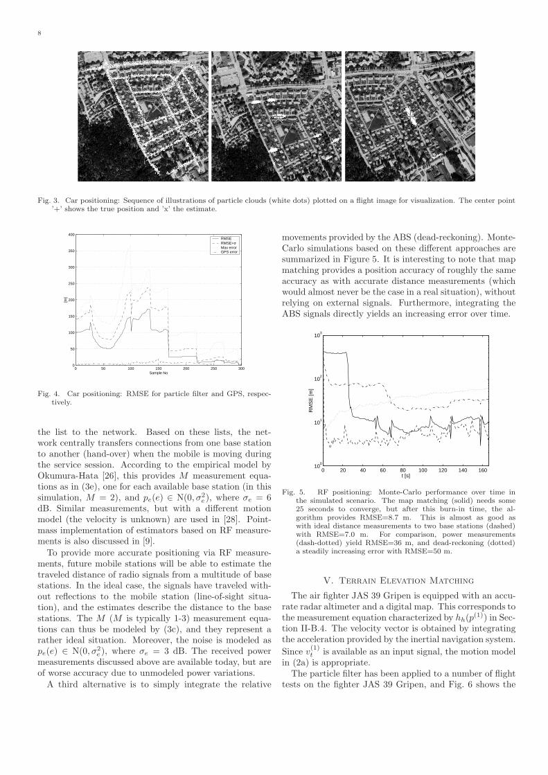
Fig. 3 shows a sequence of images of the particle cloudon a flight image of the local area. The driven path consistsof a number of 90 degrees turns. Initially, the particles arespread uniformly over all admissible positions, that is, onthe roads, covering an area of about one square kilometer.After the first turns, a few clouds are left. After 4–5 turns,the filter essentially has converged. One can note that thestate evolution on the straight path extends the cloud alongthe road to take into account unprecise velocity informa-tion. Details of the implementation are found in [23], [25],while some comments on the divergence problem are givenin the conclusions.

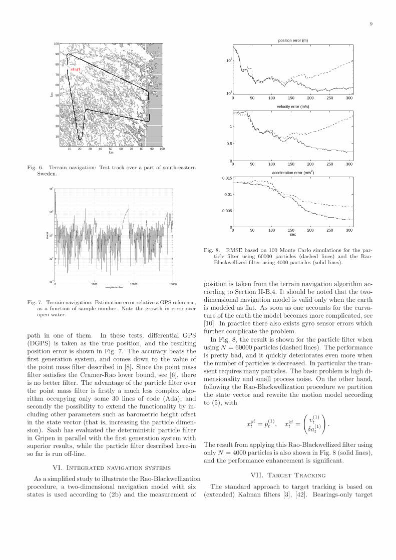
GPS is used as a reference positioning system. It pro-vides reliable position estimates in rural areas, but is ham-pered in non line-of-sight situations and when the signalsare attenuated by foliage etc. After convergence, the mapmatching particle filter is seen equal to, or even slightlybetter than, GPS in terms of performance, see Fig. 4. How-ever, in test drives along forests, close to high buildings andtunnels, the GPS performance deteriorates quickly. Fur-thermore, the GPS has a convergence time of about 45seconds when turned on, not shown in Fig. 4.

For comparison, the particle filter using map matchingand filters based on measurements from a fictive terrestrialwireless communications system are applied to data from asimulation setup mimicking the real case above. The areais essentially covered by one macro cell, but yet anotherbase station is assumed within measurable distance.

The base stations in a terrestrial wireless communica-tions system act as beacons by transmitting pilot signals ofknown power. The mobile station monitors the M (in GSM(Global System for Mobile Communications), M = 5)strongest signals, and reports regularly (or event-driven)

8

Fig. 3. Car positioning: Sequence of illustrations of particle clouds (white dots) plotted on a flight image for visualization. The center point’+’ shows the true position and ’x’ the estimate.

0 50 100 150 200 250 3000

50

100

150

200

250

300

350

400

Sample No

[m]

RMSE RMSE+σMax error GPS error

Fig. 4. Car positioning: RMSE for particle filter and GPS, respec-tively.

the list to the network. Based on these lists, the net-work centrally transfers connections from one base stationto another (hand-over) when the mobile is moving duringthe service session. According to the empirical model byOkumura-Hata [26], this provides M measurement equa-tions as in (3e), one for each available base station (in thissimulation, M = 2), and pe(e) ∈ N(0, σ2

e), where σe = 6dB. Similar measurements, but with a different motionmodel (the velocity is unknown) are used in [28]. Point-mass implementation of estimators based on RF measure-ments is also discussed in [9].

To provide more accurate positioning via RF measure-ments, future mobile stations will be able to estimate thetraveled distance of radio signals from a multitude of basestations. In the ideal case, the signals have traveled with-out reflections to the mobile station (line-of-sight situa-tion), and the estimates describe the distance to the basestations. The M (M is typically 1-3) measurement equa-tions can thus be modeled by (3c), and they represent arather ideal situation. Moreover, the noise is modeled aspe(e) ∈ N(0, σ2

e), where σe = 3 dB. The received powermeasurements discussed above are available today, but areof worse accuracy due to unmodeled power variations.

A third alternative is to simply integrate the relative

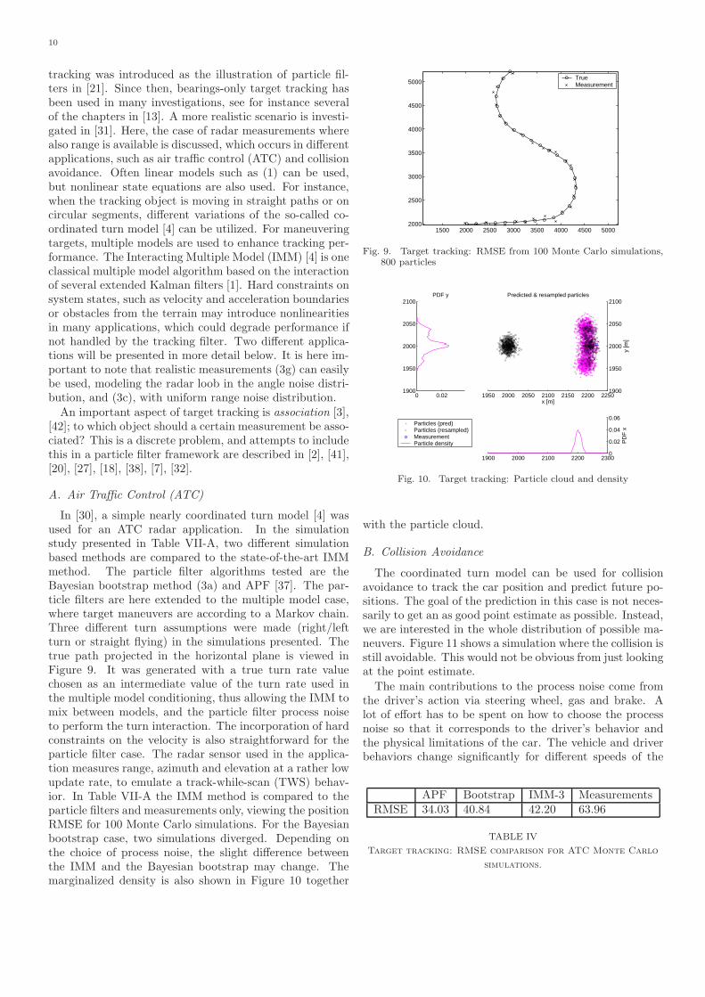
movements provided by the ABS (dead-reckoning). Monte-Carlo simulations based on these different approaches aresummarized in Figure 5. It is interesting to note that mapmatching provides a position accuracy of roughly the sameaccuracy as with accurate distance measurements (whichwould almost never be the case in a real situation), withoutrelying on external signals. Furthermore, integrating theABS signals directly yields an increasing error over time.

0 20 40 60 80 100 120 140 16010

0

101

102

103

t [s]

RM

SE

[m]

Fig. 5. RF positioning: Monte-Carlo performance over time inthe simulated scenario. The map matching (solid) needs some25 seconds to converge, but after this burn-in time, the al-gorithm provides RMSE=8.7 m. This is almost as good aswith ideal distance measurements to two base stations (dashed)with RMSE=7.0 m. For comparison, power measurements(dash-dotted) yield RMSE=36 m, and dead-reckoning (dotted)a steadily increasing error with RMSE=50 m.

V. Terrain Elevation Matching

The air fighter JAS 39 Gripen is equipped with an accu-rate radar altimeter and a digital map. This corresponds tothe measurement equation characterized by hh(p(1)) in Sec-tion II-B.4. The velocity vector is obtained by integratingthe acceleration provided by the inertial navigation system.Since v(1)

t is available as an input signal, the motion modelin (2a) is appropriate.

The particle filter has been applied to a number of flighttests on the fighter JAS 39 Gripen, and Fig. 6 shows the

9

10 20 30 40 50 60 70 80 90 100

10

20

30

40

50

60

70

80

90

100

start

km

km

Fig. 6. Terrain navigation: Test track over a part of south-easternSweden.

0 5000 10000 1500010

−1

100

101

102

103

met

er

samplenumber

Fig. 7. Terrain navigation: Estimation error relative a GPS reference,as a function of sample number. Note the growth in error overopen water.

path in one of them. In these tests, differential GPS(DGPS) is taken as the true position, and the resultingposition error is shown in Fig. 7. The accuracy beats thefirst generation system, and comes down to the value ofthe point mass filter described in [8]. Since the point massfilter satisfies the Cramer-Rao lower bound, see [6], thereis no better filter. The advantage of the particle filter overthe point mass filter is firstly a much less complex algo-rithm occupying only some 30 lines of code (Ada), andsecondly the possibility to extend the functionality by in-cluding other parameters such as barometric height offsetin the state vector (that is, increasing the particle dimen-sion). Saab has evaluated the deterministic particle filterin Gripen in parallel with the first generation system withsuperior results, while the particle filter described here-inso far is run off-line.

VI. Integrated navigation systems

As a simplified study to illustrate the Rao-Blackwellizationprocedure, a two-dimensional navigation model with sixstates is used according to (2b) and the measurement of

0 50 100 150 200 250 30010

1

102

position error (m)

0 50 100 150 200 250 3000

0.5

1

velocity error (m/s)

0 50 100 150 200 250 3000

0.005

0.01

0.015acceleration error (m/s2)

sec

Fig. 8. RMSE based on 100 Monte Carlo simulations for the par-ticle filter using 60000 particles (dashed lines) and the Rao-Blackwellized filter using 4000 particles (solid lines).

position is taken from the terrain navigation algorithm ac-cording to Section II-B.4. It should be noted that the two-dimensional navigation model is valid only when the earthis modeled as flat. As soon as one accounts for the curva-ture of the earth the model becomes more complicated, see[10]. In practice there also exists gyro sensor errors whichfurther complicate the problem.

In Fig. 8, the result is shown for the particle filter whenusing N = 60000 particles (dashed lines). The performanceis pretty bad, and it quickly deteriorates even more whenthe number of particles is decreased. In particular the tran-sient requires many particles. The basic problem is high di-mensionality and small process noise. On the other hand,following the Rao-Blackwellization procedure we partitionthe state vector and rewrite the motion model accordingto (5), with

xpft = p

(1)t , xkf

t =

(v

(1)t

δa(1)t

).

The result from applying this Rao-Blackwellized filter usingonly N = 4000 particles is also shown in Fig. 8 (solid lines),and the performance enhancement is significant.

VII. Target Tracking

The standard approach to target tracking is based on(extended) Kalman filters [3], [42]. Bearings-only target

10

tracking was introduced as the illustration of particle fil-ters in [21]. Since then, bearings-only target tracking hasbeen used in many investigations, see for instance severalof the chapters in [13]. A more realistic scenario is investi-gated in [31]. Here, the case of radar measurements wherealso range is available is discussed, which occurs in differentapplications, such as air traffic control (ATC) and collisionavoidance. Often linear models such as (1) can be used,but nonlinear state equations are also used. For instance,when the tracking object is moving in straight paths or oncircular segments, different variations of the so-called co-ordinated turn model [4] can be utilized. For maneuveringtargets, multiple models are used to enhance tracking per-formance. The Interacting Multiple Model (IMM) [4] is oneclassical multiple model algorithm based on the interactionof several extended Kalman filters [1]. Hard constraints onsystem states, such as velocity and acceleration boundariesor obstacles from the terrain may introduce nonlinearitiesin many applications, which could degrade performance ifnot handled by the tracking filter. Two different applica-tions will be presented in more detail below. It is here im-portant to note that realistic measurements (3g) can easilybe used, modeling the radar loob in the angle noise distri-bution, and (3c), with uniform range noise distribution.

An important aspect of target tracking is association [3],[42]; to which object should a certain measurement be asso-ciated? This is a discrete problem, and attempts to includethis in a particle filter framework are described in [2], [41],[20], [27], [18], [38], [7], [32].

A. Air Traffic Control (ATC)

In [30], a simple nearly coordinated turn model [4] wasused for an ATC radar application. In the simulationstudy presented in Table VII-A, two different simulationbased methods are compared to the state-of-the-art IMMmethod. The particle filter algorithms tested are theBayesian bootstrap method (3a) and APF [37]. The par-ticle filters are here extended to the multiple model case,where target maneuvers are according to a Markov chain.Three different turn assumptions were made (right/leftturn or straight flying) in the simulations presented. Thetrue path projected in the horizontal plane is viewed inFigure 9. It was generated with a true turn rate valuechosen as an intermediate value of the turn rate used inthe multiple model conditioning, thus allowing the IMM tomix between models, and the particle filter process noiseto perform the turn interaction. The incorporation of hardconstraints on the velocity is also straightforward for theparticle filter case. The radar sensor used in the applica-tion measures range, azimuth and elevation at a rather lowupdate rate, to emulate a track-while-scan (TWS) behav-ior. In Table VII-A the IMM method is compared to theparticle filters and measurements only, viewing the positionRMSE for 100 Monte Carlo simulations. For the Bayesianbootstrap case, two simulations diverged. Depending onthe choice of process noise, the slight difference betweenthe IMM and the Bayesian bootstrap may change. Themarginalized density is also shown in Figure 10 together

1500 2000 2500 3000 3500 4000 4500 50002000

2500

3000

3500

4000

4500

5000True Measurement

Fig. 9. Target tracking: RMSE from 100 Monte Carlo simulations,800 particles

1950 2000 2050 2100 2150 2200 22501900

1950

2000

2050

2100Predicted & resampled particles

x [m]

y [m

]

Particles (pred) Particles (resampled)Measurement Particle density

0 0.021900

1950

2000

2050

2100PDF y

1900 2000 2100 2200 23000

0.02

0.04

0.06

PD

F x

Fig. 10. Target tracking: Particle cloud and density

with the particle cloud.

B. Collision Avoidance

The coordinated turn model can be used for collisionavoidance to track the car position and predict future po-sitions. The goal of the prediction in this case is not neces-sarily to get an as good point estimate as possible. Instead,we are interested in the whole distribution of possible ma-neuvers. Figure 11 shows a simulation where the collision isstill avoidable. This would not be obvious from just lookingat the point estimate.

The main contributions to the process noise come fromthe driver’s action via steering wheel, gas and brake. Alot of effort has to be spent on how to choose the processnoise so that it corresponds to the driver’s behavior andthe physical limitations of the car. The vehicle and driverbehaviors change significantly for different speeds of the

APF Bootstrap IMM-3 MeasurementsRMSE 34.03 40.84 42.20 63.96

TABLE IV

Target tracking: RMSE comparison for ATC Monte Carlo

simulations.

11

0 10 20 30 40 50 60 70−20

−15

−10

−5

0

5

10

15

20

Fig. 11. Collision avoidance: The left rectangle is the own car, whichis approaching rapidly the right rectangle. The trajectories indi-cate 31-step ahead prediction using 100 particles. There are stillpossible trajectories avoiding collision, of which the driver willmost probably choose one. Thus, no active control is needed atthis stage.

vehicle. Thus, in order to get a good prediction with thismodel, it is necessary to let the process noise ft change withdifferent speeds. It is also important in this application toincorporate knowledge about the environment to improvethe prediction. For example, it is likely that the car willtravel on the road and if there are some hard boundarieslike rails or other stationary objects these are hard con-straints on the car’s movement.

VIII. Conclusions and Discussion

We have given a general framework for positioning andnavigation applications based on a flexible state spacemodel and a particle filter. Five applications illustrate itsuse in practice. Evaluations in real-time, off-line on realdata and in simulation environments show a clear improve-ment in performance compared to existing Kalman filterbased solutions, where the new challenge is to find non-linear relations, state constraints and non-Gaussian sensormodels that provide the most information about the po-sition. Thus, modeling is the most essential step in thisapproach, compared to the various implementations of theKalman filter found in this context (linearization issues,choice of state co-ordinates, filter banks, Gaussian sum fil-ters, etc.).

General conclusions from the implementations are as fol-lows: A choice of state coordinates making the state equa-tion linear is beneficial for computation time and opensup the possibility for Rao-Blackwellization. This proce-dure enables a significant decrease in the particle state di-mension. The evaluation of the likelihood one step aheadbefore re-sampling (APF, prior editing) is, together withadding extra state noise (jittering, roughening), crucial foravoiding divergence, and implies that the number of par-ticles can be decreased further. Our implementations runin real-time (2Hz), even in Matlab, and have some 2000particles.

Open questions for further research and development are

listed below:• Divergence tests. It is essential to have a reliable way todetect divergence and to restart the filter (for the latter, seethe transient below). For car positioning, the number of re-samplings in the prior editing step turned out to be a verygood indicator of divergence. Another idea, used in theterrain navigation implementation where the sampling rateis higher than necessary, is to split up the measurements toa filter bank, so that particle filter number i, i = 1, 2, . . . , ngets every n’th sample. The result of these n particle filtersare approximately independent and voting can be used torestart each filter. This has turned out to be an efficientway to remove the outliers in data.• Transient improvement. The time it takes until the es-timate accuracy comes down to the stationary value (theCramer-Rao bound) depends on the number of particles.Given limited computational time, it may be advantageousto increase the number of particles N after a restart anddiscard samples in such a way that N/Ts is constant.• Since the particle filter has shown good improvement overlinearization approaches, it is tempting to try even more ac-curate non-linear models. In particular, the flight dynamicsof one’s own vehicle is known and indeed used in model-based control, but is very rare in navigation applications,see [33] for one attempt in this direction. In that study,it seems that the computational burden and linearizationerrors imply no gain in total performance. As a possibleimprovement, the particle filter may take full advantageof a more accurate model, where parts of the non-lineardynamics from driver/pilot inputs are incorporated.

Acknowledgment

The competence center ISIS at Linkoping University hasbrought all of the authors together and provides funding forRickard and Per-Johan. We are very grateful to ChristopheAndrieu and Arnoud Doucet for our fruitful discussionson the theoretical subjects. We want to acknowledge ourgratitude to the master students Magnus Ahlstrom, MarcusCalais, who have implemented the terrain navigation filter,and Peter Hall, who implemented the car positioning filter,and the supporting companies SAAB Dynamics and NIRADynamics, respectively.

Appendix

For the derivation of the Rao-Blackwellized algorithmgiven in Section III-D, suppose first that the particle filterpart of the state vector is known. That is, the sequenceXpft = {xpf

0 , . . . , xpft } is known. We can, temporally, con-

sider zt = xpft+1− x

pft as the measurement. The state space

model is here

xkft+1 = Akfxkf

t +Bkfu ut +Bkf

f ft

zt = Apfxkft +Bpf

u ut +Bpff ft.

Since this model is linear and Gaussian, the optimal solu-tion is provided by the Kalman filter. We then know thatp(xkf

t |Xpft ) is Gaussian, so

xkft |X

pft = xkf

t |Zt−1 ∼ N(xkft|t−1, P

kft|t−1),

12

where xkft|t−1 and P kft|t−1 are given by the Kalman filter equa-tions adjusted for correlated noise [24],

Kt =P kft|t−1(Apf)T (ApfP kf

t|t−1(Apf)T +Bpff Qt(B

pff )T )−1

xkft+1|t =A

kf(xkft|t−1 +Kt(zt −Apf xkf

t|t−1)) +

Bkfu ut +Bkf

f (Bpff )†zt

P kft+1|t =A

kf(P kft|t−1 −KtA

pfP kft|t−1)(A

kf)T ,

where Akf

= Akf − Bkff (Bpf

f )†Apf († denotes the Moore-Penrose pseudo-inverse).

Now, to compute p(xt|Yt) = p(xpft , x

kft |Yt), note that

p(Xpft , x

kft |Yt) = p(xkf

t |Xpft )p(Xpf

t |Yt).

We only have to compute p(Xpft |Yt). Repeated use of

Bayes’ rule gives

p(Xpft |Yt) =

p(yt|xpft )p(xpf

t |Xpft−1)

p(yt|Yt−1)p(Xpf

t−1|Yt−1).

We have a nonlinear and non-Gaussian measurement equa-tion, so to solve the measurement update, the particle filterwill be used to approximate this distribution. The particlepredictions p(xpf

t+1|Xpft ) are given by

xpft+1|X

pft = xpf

t +Apfxkft |X

pft +Bpf

u ut +Bpff ft,

so p(xpft+1|X

pft ) is given by

N(xpft +Apf xkf

t|t−1 + Bpfu ut,

ApfP kft|t−1(Apf)T +Bpf

f Qt(Bpff )T ).

Finally, note that the derivation does not change if we usethe fictitious measurement zt = xpf

t+1 − g(xpft ) for an arbi-

trary non-linear function, which is Remark 3.

Fredrik Gustafsson is professor in Commu-nication Systems at the Department of Elec-trical Engineering at Linkoping University. Hereceived the M.S. degree in electrical engineer-ing in 1988 and the Ph.D. degree in automaticcontrol in 1992, both from Linkoping Univer-sity, Sweden. His research is focused on sta-tistical methods in signal processing, with ap-plications to automotive, avionic and commu-nication systems. He is an associate editor ofIEEE Transactions of Signal Processing.

Fredrik Gunnarsson is a research associateat Communications Systems, Department ofElectrical Engineering, Linkoping University.He received the M.Sc. degree in applied physicsand electrical engineering in 1996 and thePh.D. degree in electrical engineering in 2000,both from Linkoping University, Sweden. Hisresearch interests include control and signal

processing in terrestrial wireless communica-tions systems and automotive applications.

Niclas Bergman is with SaabTech Systems.He received his M.Sc. degree in applied physicsand electrical engineering in 1995 and thePh.D. degree in electrical engineering in 1999,both from Linkoping University, Sweden. He iscurrently working with research and develop-ment in the areas of target tracking and navi-gation, and responsible for the coordination ofdata fusion activities within the Saab group.

Urban Forssell Urban Forssell is presidentand CEO of NIRA Dynamics AB. The com-pany focuses on advanced signal processing andcontrol in vehicles. He received his M.Sc. de-gree in applied physics and electrical engineer-ing in 1995 and the Ph.D. degree in automaticcontrol in 1999, both from Linkoping Univer-sity, Sweden.

Jonas Jansson is employed at Volvo Car Cor-poration with developing a collision avoidancesystem. He is since 1999 spending 50% of histime as a PhD student at Linkoping University.His current research interests focus on particlefilter implementation of navigation and track-ing systems.

Rickard Karlsson has worked at SAAB Dy-namics with target tracking and sensor fusionsince 1997. He is since 1999 spending half histime as a PhD student at Linkoping University.His current research interests focus on particlefilter implementation of target tracking algo-rithms with radar and/or IR sensors.

13

Per-Johan Nordlund has worked at SAABGripen with developing a new version of thenavigation system for the fighter JAS 39Gripen for several years. He is since 1999spending 75% of his time as a PhD studentat Linkoping University. His current researchinterests focus around particle filter implemen-tation of integrated navigation systems withparticular attention to complexity aspects andfault detection.

References

[1] B.D.O. Anderson and J.B. Moore. Optimal filtering. PrenticeHall, Englewood Cliffs, NJ., 1979.

[2] D. Avitzour. Stochastic simulation Bayesian approach to mul-titarget tracking. IEE Proc. on Radar, Sonar and Navigation,142(2), 1995.

[3] Y. Bar-Shalom and T. Fortmann. Tracking and Data Associ-ation, volume 179 of Mathematics in Science and Engineering.Academic Press, 1988.

[4] Y. Bar-Shalom and X.R. Li. Estimation and tracking: princi-ples, techniques, and software. Artech House, 1993.

[5] N. Bergman. Recursive Bayesian Estimation: Navigation andTracking Applications. Dissertation nr. 579, Linkoping Univer-sity, Sweden, 1999.

[6] N. Bergman. Posterior Cramer-Rao bounds for sequential esti-mation. In A. Doucet, N. de Freitas, and N. Gordon, editors,Sequential Monte Carlo Methods in Practice. Springer-Verlag,2001.

[7] N. Bergman and A. Doucet. Markov Chain Monte Carlo data as-sociation for target tracking. In IEEE Conference on Acoustics,Speech and Signal Processing, 2000.

[8] N. Bergman, L. Ljung, and F. Gustafsson. Terrain naviga-tion using Bayesian statistics. IEEE Control System Magazine,19(3):33–40, 1999.

[9] J. Blom, F. Gunnarsson, and F. Gustafsson. Estimation in cel-lular radio systems. In Proc. IEEE International Conference onAcoustics, Speech, and Signal Processing., Phoenix, AZ, USA.,March 1999.

[10] K.R. Britting. Inertial Navigation Systems Analysis. Wiley -Interscience, 1971.

[11] D. Crisan and A. Doucet. Convergence of sequential MonteCarlo methods. Technical Report CUED/F-INFENG/TR381,Signal Processing Group, Department of Engineering, Univer-sity of Cambridge, 2000.

[12] A. Doucet and C. Andrieu. Particle filtering for partially ob-served Gaussian state space models. Technical Report CUED/F-INFENG/TR393, Department of Engineering, University ofCambridge CB2 1PZ Cambridge, September 2000.

[13] A. Doucet, N. de Freitas, and N. Gordon, editors. SequentialMonte Carlo Methods in Practice. Springer Verlag, 2001.

[14] A. Doucet, S.J. Godsill, and C. Andrieu. On sequentialsimulation-based methods for Bayesian filtering. Statistics andComputing, 10(3):197–208, 2000.

[15] A. Doucet, N.J. Gordon, and V. Krishnamurthy. Particle Filtersfor State Estimation of Jump Markov Linear Systems. IEEETrans. on Signal Processing, 49(3):613–624, March 2001.

[16] C. Drane, M. Macnaughtan, and C. Scott. Positioning GSMtelephones. IEEE Communications Magazine, 36(4), 1998.

[17] P. Fearnhead. Sequential Monte Carlo methods in filter theory.PhD thesis, University of Oxford, 1998.

[18] S. Geman and D. Geman. Stochastic relaxation, Gibbs distribu-tions and the Bayesian restoration of images. IEEE Trans. onPattern Analysis and Machine Intelligence, 6:721–741, 1984.

[19] W. Gilks, S. Richardson, and D. Spiegelhalter. Markov ChainMonte Carlo in practice. Chapman & Hall, 1996.

[20] N.J. Gordon. A hybrid bootstrap filter for target tracking in clut-ter. In IEEE Transactions on Aerospace and Electronic Systems,volume 33, pages 353–358, 1997.

[21] N.J. Gordon, D.J. Salmond, and A.F.M. Smith. A novel ap-proach to nonlinear/non-Gaussian Bayesian state estimation. InIEE Proceedings on Radar and Signal Processing, volume 140,pages 107–113, 1993.

[22] F. Gustafsson, S. Ahlqvist, U. Forssell, and N. Persson. Sen-sor fusion for accurate computation of yaw rate and absolutevelocity. In SAE 2001, Detroit, 2001.

[23] F. Gustafsson, U. Forssell, and P. Hall. Car positioning system.Swedish patent application nr SE0004096-4, 2000.

[24] Fredrik Gustafsson. Adaptive filtering and change detection.John Wiley & Sons, Ltd, 2000.

[25] P. Hall. A Bayesian approach to map-aided vehicle positioning.Master Thesis LiTH-ISY-EX-3104, Dept of Elec. Eng. LinkopingUniversity, S-581 83 Linkoping, Sweden, 2001. In Swedish.

[26] M. Hata. Empirical formula for propagation loss in land mo-bile radio services. IEEE Transactions on Vehicular Technology,29(3), 1980.

[27] C. Hue, J.P. Le Cadre, and P. Perez. Tracking multiple objectswith particle filtering. Technical report, Research report IRISA,No1361, Oct 2000.

[28] H. Jwa, S. Kim, X. Cho, and J. Chun. Position tracking ofmobiles in a cellular radio network using the constrained boot-strap filter. In Proc. National Aerospace Electronics Conference,Dayton, OH, USA, October 2000.

[29] T. Kailath, A.H. Sayed, and B. Hassibi. Linear estimation. Infor-mation and System Sciences. Prentice-Hall, Upper Saddle River,New Jersey, 2000.

[30] R. Karlsson and N. Bergman. Auxiliary particle filters for track-ing a maneuvering target. In IEEE Conference on Decision andControl, Sydney, Australia, Dec 2000.

[31] R. Karlsson and F. Gustafsson. Range estimation using angle-only target tracking with particle filters. In Proc. of the Ameri-can Control Conference, Arlington, Virginia, U.S.A, June 2001.

[32] Rickard Karlsson and Fredrik Gustafsson. Monte Carlo dataassociation for multiple target tracking. In IEE Target tracking:Algorithms and applications, The Netherlands, Oct 2001.

[33] M. Koifman and I.Y. Bar-Itzhack. Inertial navigation systemaided by aircraft dynamics. IEEE Transactions on Control Sys-tems Technology, 7(4):487–493, 1999.

[34] A. Kong, J. S. Liu, and W. H. Wong. Sequential imputationsand Bayesian missing data problems. J. Amer. Stat. Assoc.,89(425):278–288, 1994.

[35] J.S. Liu. Metropolized independent sampling with comparisonto rejection ampling and importance sampling. Statistics andComputing, 6:113–119, 1996.

[36] P-J. Nordlund and F. Gustafsson. Sequential monte carlo fil-tering techniques applied to integrated navigation systems. InProc. of the American Control Conference, Arlington, Virginia,U.S.A, June 2001.

[37] M.K. Pitt and N. Shephard. Filtering via simulation: Auxiliaryparticle filters. Journal of the American Statistical Association,94(446):590–599, June 1999.

[38] C. Rago, P.Willett, and R.Streit. A comparison of the JPDAFand PMHT tracking algorithms. In IEEE Conference on Acous-tics, Speech and Signal Processing, volume 5, pages 3571–3574,1995.

[39] B.D. Ripley. Stochastic Simulation. John Wiley, 1988.[40] S. Rohr, R. Lind, R. Myers, W. Bauson, W. Kosiak, and H. Yen.

An integrated approach to automotive safety systems. Automo-tive engineering international, September 2000.

[41] D.J Salmond, D. Fisher, and N.J Gordon. Tracking in the pres-ence of intermittent spurious objects and clutter. In SPIE Conf.on Signal and Data Processing of Small Tragets, 1998.

[42] Blackman S.S and Popoli R. Design and analysis of moderntracking systems. Artech House, Norwood, MA, 1999.

[43] S. Thrun, D. Fox, F. Dellaert, and W. Burgard. Particle filtersfor mobile robot localization. In A. Doucet, N. de Freitas, andN. Gordon, editors, Sequential Monte Carlo Methods in Prac-tice. Springer-Verlag, 2001.

[44] O. Wijk. Triangulation Based Fusion of Sonar Data with Appli-cation in Mobile Robot Mapping and Localization. PhD thesis,Royal Institute of Technology, 2001.