1

RISK

MANAGEMENT AT

THE

CAISSE DE D

ÉPÔT ET

PLACEMENT DU Q

UÉBEC

Presented by: Susan Kudzman, FSA, FCIA

Executive Vice PresidentDepositors and Risks

Pension seminarCanadian Institute of Actuaries

April 15, 2008

2

01The Caisse

02Governance and division of responsibilities

03Risk model

04Value at risk

05Other concepts of risk

06Annexes

3

THE CAISSE

01

4

1. The Caisse at a glance

> The Caisse is one of the leading institutional fund managers in Canada and North America

> Net assets under management totalling $155.4 billion (as at December 31, 2007)

> Total transactions carried out daily exceeding $12 billion

> A shareholder in over 3 000 businesses internationally

> One of the world’s 10 largest real estate asset managers

5

1. The Caisse:its mission, its values

ITS MISSION

To make profitable investments with the funds of public and private pension and insurance plans and organizations, while contributing to Quebec’s economic development. These organizations are the Caisse’s ”clients”, which it calls its depositors.

ITS VALUES> excellence> ethics> boldness> transparency

ITS AMBITION> Become a benchmark organization so as to stand apart from the other leading institutional fund managers.

6

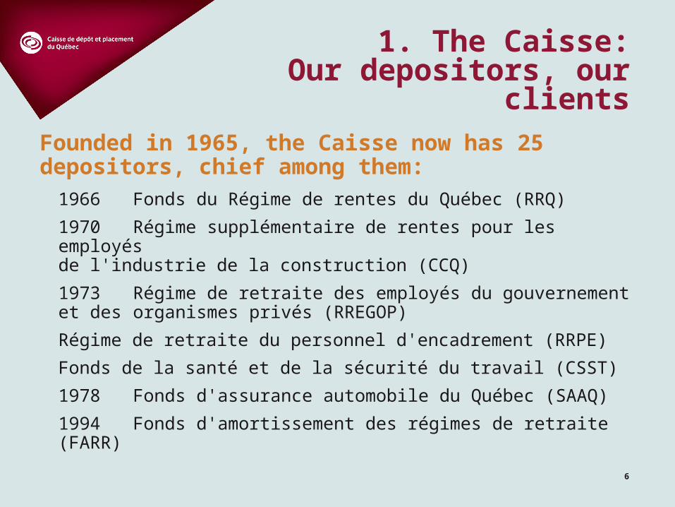
1. The Caisse:Our depositors, our clients

Founded in 1965, the Caisse now has 25 depositors, chief among them:

1966 Fonds du Régime de rentes du Québec (RRQ)

1970 Régime supplémentaire de rentes pour les employés de l'industrie de la construction (CCQ)

1973 Régime de retraite des employés du gouvernement et des organismes privés (RREGOP)

Régime de retraite du personnel d'encadrement (RRPE)

Fonds de la santé et de la sécurité du travail (CSST)

1978 Fonds d'assurance automobile du Québec (SAAQ)

1994 Fonds d'amortissement des régimes de retraite (FARR)

7

GOVERNANCE AND

DIVISION O

F

RESPONSIBILITIES

02

8

2. Governance and division of responsibilities

PHILOSOPHY: Promote a strong risk management culture and practices that help the Caisse fulfil its obligations toward its depositors

OBJECTIVES:> Avoid undue losses in the Caisse’s and depositors’ portfolios> Provide guidelines as to the level of risk that the Caisse is prepared

to assume in carrying out its mission and complying with its depositors’ investment policies.

> Ensure that targets are in line with the risks assumed.> Assign risk limits effectively among the various investment groups> Establish clear responsibilities for risk management.

Integrated Risk Management Policy (IRMP)

9

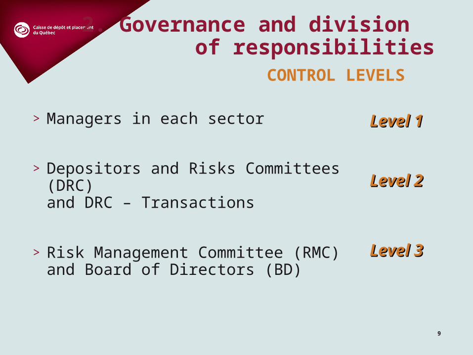
2. Governance and division of responsibilities

> Managers in each sector

> Depositors and Risks Committees (DRC) and DRC – Transactions

> Risk Management Committee (RMC) and Board of Directors (BD)

Level 1Level 1

Level 2Level 2

Level 3Level 3

CONTROL LEVELS

10

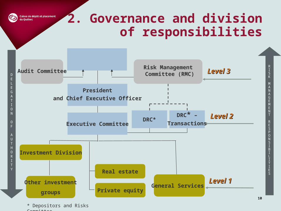
DELEGATION

OF

AUTHORITY

2. Governance and division of responsibilities

Level 1Level 1

Level 2Level 2

Level 3Level 3

Board of Directors

President

and Chief Executive Officer

Other investment

groupsGeneral Services

DRC*

Audit Committee

* Depositors and Risks Committee

Risk Management Committee (RMC)

Executive Committee

DRC* –

Transactions

Investment Division

Real estate

Private equity

RISK

MANAGEMENT

RESPONSIBILITIES

11

2. Governance and division of responsibilities

MANAGERS IN EACH SECTOR (LEVEL 1)> Define and put in place the controls needed to ensure compliance

with the procedures outlined in the IRMP, including investment policies and the attendant directives.

> Specifically for investment group managers:• Organize specialized portfolios (management assignments and

risk management)

> Give authorization for management assignment limits to be exceeded within their respective area of delegation and inform the DRC

> Submit to DRC – Transactions those investments that exceed their level of authority

12

2. Governance and division of responsibilities

DRC AND DRC – TRANSACTIONS (LEVEL 2)

DRC:

> Ensure optimal organization of risk management> Recommend investment policies to the Board of

Directors> Approve directives> Monitor risks (market, credit, liquidity and operational

risks)DRC – Transactions:

> Analyse, approve or recommend transactions

13

2. Governance and division of responsibilities

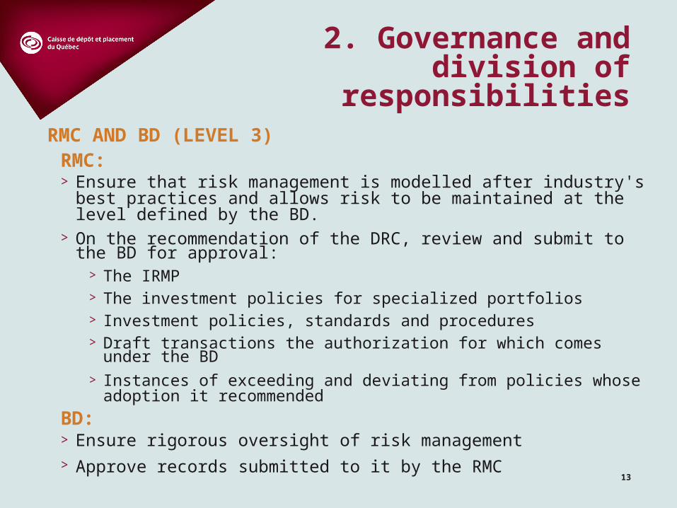
RMC AND BD (LEVEL 3)RMC:> Ensure that risk management is modelled after industry's best practices and

allows risk to be maintained at the level defined by the BD.> On the recommendation of the DRC, review and submit to the BD for

approval:> The IRMP> The investment policies for specialized portfolios> Investment policies, standards and procedures > Draft transactions the authorization for which comes under the BD> Instances of exceeding and deviating from policies whose adoption it

recommended

BD:> Ensure rigorous oversight of risk management> Approve records submitted to it by the RMC

14

RISK MODEL

03

15

3. Risk model

Why a risk model? > Identifies the risks to which the organization is exposed

> In a structured way, classifies the information gathered on risks so as to be able to analyse it

> All the stakeholders use the same language in order to communicate better with respect to risks

The basis on which integrated risk management is designed

16

3. Risk model

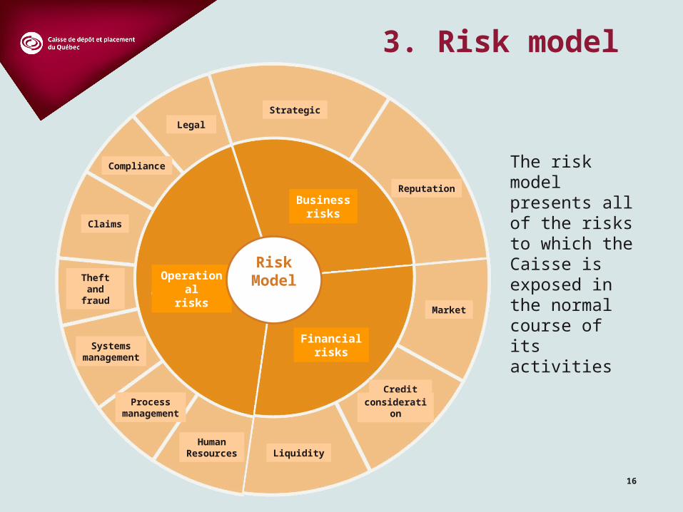
The risk model presents all of the risks to which the Caisse is exposed in the normal course of its activities

Strategic

Reputation

Market

Credit andconsideration

LiquidityHuman

Resources

Processmanagement

Systemsmanagement

Theft andfraud

Claims

Compliance

Legal

Operationalrisks

Financialrisks

Businessrisks

RiskModel

17

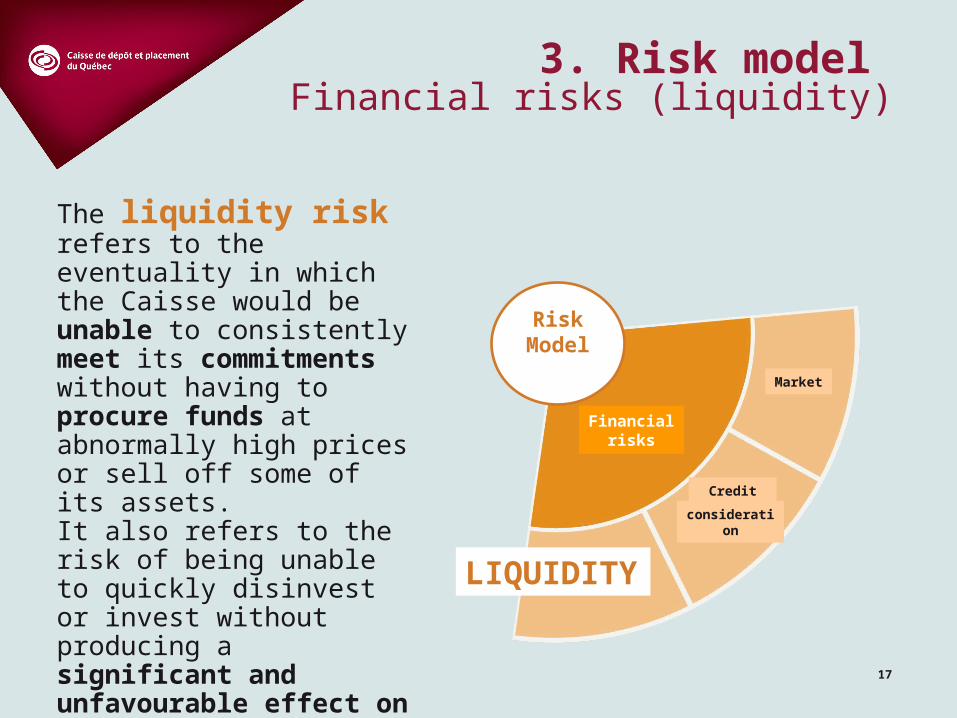
3. Risk model Financial risks (liquidity)

The liquidity risk refers to the eventuality in which the Caisse would be unable to consistently meet its commitments without having to procure funds at abnormally high prices or sell off some of its assets.It also refers to the risk of being unable to quickly disinvest or invest without producing a significant and unfavourable effect on the price of the investment in question

LIQUIDITY

Financialrisks

Credit and

consideration

Market

RiskModel

18

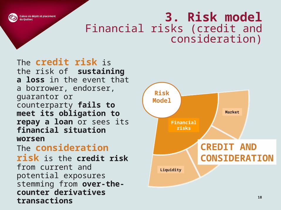
3. Risk modelFinancial risks (credit and consideration)

The credit risk is the risk of sustaining a loss in the event that a borrower, endorser, guarantor or counterparty fails to meet its obligation to repay a loan or sees its financial situation worsen The consideration risk is the credit risk from current and potential exposures stemming from over-the-counter derivatives transactions

CREDIT ANDCONSIDERATION

Financialrisks

Market

Liquidity

RiskModel

19

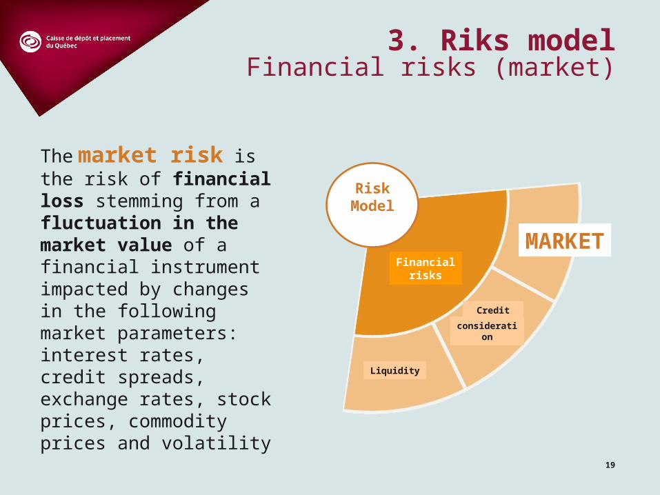
3. Riks modelFinancial risks (market)

MARKET

The market risk is the risk of financial loss stemming from a fluctuation in the market value of a financial instrument impacted by changes in the following market parameters: interest rates, credit spreads, exchange rates, stock prices, commodity prices and volatility

Financialrisks

Liquidity

Credit and

consideration

RiskModel

20

VALUE

AT RISK04

21

VAR

> Amount, in dollars or as a percentage, reflecting the maximum loss that can occur over a given time horizon for a desired level of confidence

> To calculate this amount, it is necessary to specify:> The time horizon

> The desired level of confidence

> Industry “standard”

4. Value at risk

22

There are three recognized approaches for obtaining a market VAR:

> Variance/covariance (parametric)

> Historical simulation (non-parametric)

> Monte Carlo simulation

Each method:

> has its specific pros and cons

> depends on certain conditions of use

4. Method of calculating VAR

23

The main difference between these three methods has to do with the assumption about the distribution of returns:

> variance/covariance → normal distribution

> historical simulation → no distribution (historical)

> Monte Carlo simulation → choice of distribution

4. Method of calculating VAR

24

PROS > No assumption about distribution of returns

> No need to estimate return correlations

> Ability to record derivatives

CONS> Estimate based on past data that might not reflect current reality

> Need for historical price series

> Additional need for IT resources

4. Method of calculating VARHistorical simulation

25

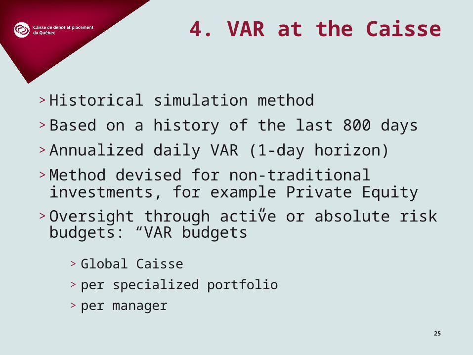
4. VAR at the Caisse

> Historical simulation method

> Based on a history of the last 800 days

> Annualized daily VAR (1-day horizon)

> Method devised for non-traditional investments, for example Private Equity

> Oversight through active or absolute risk budgets: “VAR budgets”

> Global Caisse

> per specialized portfolio

> per manager

26

OTHER CONCEPTS O

F

RISK USED A

T THE

CAISSE05

27

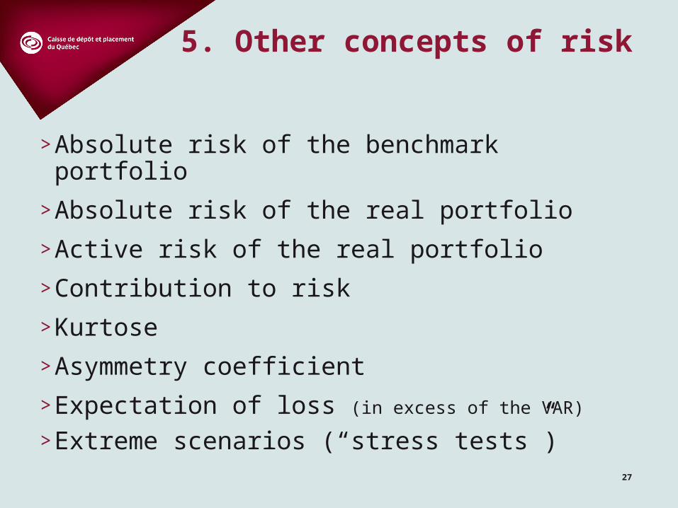
5. Other concepts of risk

>Absolute risk of the benchmark portfolio

>Absolute risk of the real portfolio

>Active risk of the real portfolio

>Contribution to risk

>Kurtose

>Asymmetry coefficient

>Expectation of loss (in excess of the VAR)

>Extreme scenarios (“stress tests”)

28

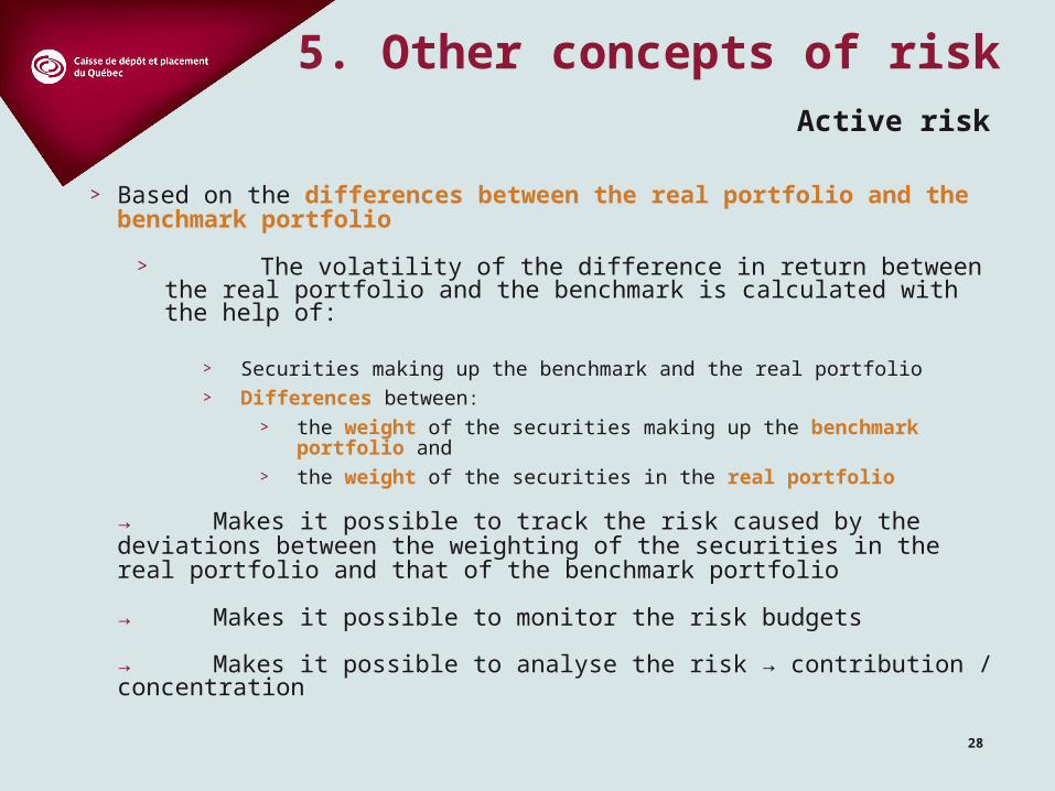
> Based on the differences between the real portfolio and the benchmark portfolio

> The volatility of the difference in return between the real portfolio and the benchmark is calculated with the help of:

> Securities making up the benchmark and the real portfolio> Differences between:

> the weight of the securities making up the benchmark portfolio and> the weight of the securities in the real portfolio

→ Makes it possible to track the risk caused by the deviations between the weighting of the securities in the real portfolio and that of the benchmark portfolio

→ Makes it possible to monitor the risk budgets

→ Makes it possible to analyse the risk → contribution / concentration

5. Other concepts of riskActive risk

29

ANNEXES

30

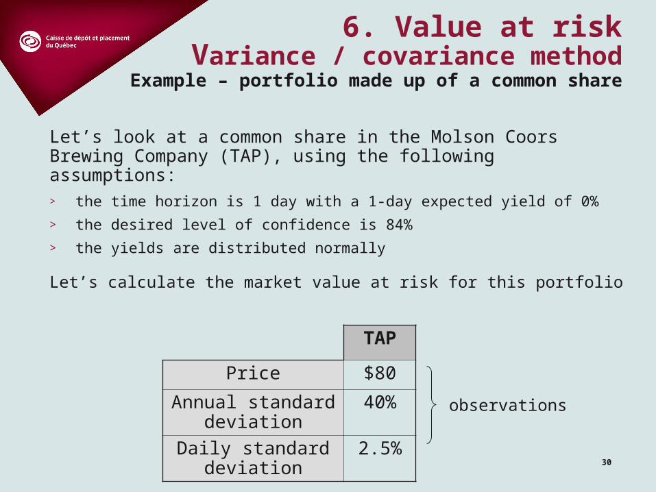
Let’s look at a common share in the Molson Coors Brewing Company (TAP), using the following assumptions:> the time horizon is 1 day with a 1-day expected yield of 0%

> the desired level of confidence is 84%

> the yields are distributed normally

Let’s calculate the market value at risk for this portfolio

TAP

Price $80

Annual standard deviation

40%

Daily standard deviation

2.5%

6. Value at riskVariance / covariance method

Example – portfolio made up of a common share

observations

31

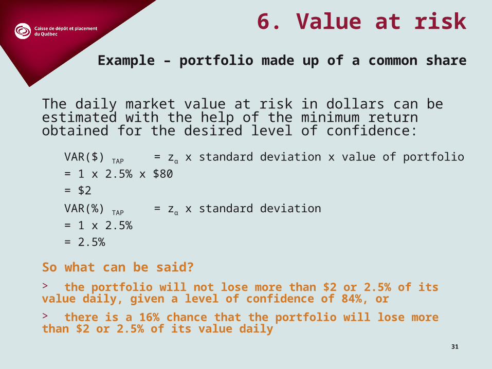
The daily market value at risk in dollars can be estimated with the help of the minimum return obtained for the desired level of confidence:

VAR($) TAP = zα x standard deviation x value of portfolio

= 1 x 2.5% x $80

= $2

VAR(%) TAP = zα x standard deviation

= 1 x 2.5%

= 2.5%

So what can be said?> the portfolio will not lose more than $2 or 2.5% of its value daily, given a level of confidence of 84%, or

> there is a 16% chance that the portfolio will lose more than $2 or 2.5% of its value daily

6. Value at risk

Example – portfolio made up of a common share

32

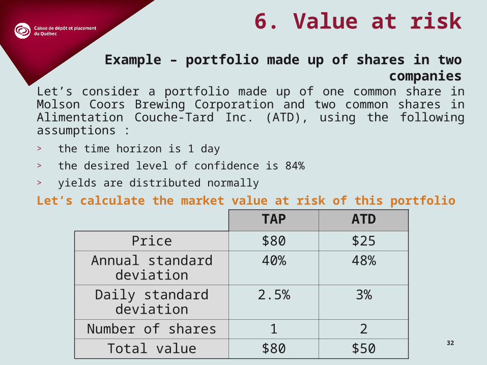
Let’s consider a portfolio made up of one common share in Molson Coors Brewing Corporation and two common shares in Alimentation Couche-Tard Inc. (ATD), using the following assumptions :

> the time horizon is 1 day

> the desired level of confidence is 84%

> yields are distributed normally

Let’s calculate the market value at risk of this portfolioTAP ATD

Price $80 $25

Annual standard deviation

40% 48%

Daily standard deviation

2.5% 3%

Number of shares 1 2

Total value $80 $50

6. Value at risk

Example – portfolio made up of shares in two companies

33

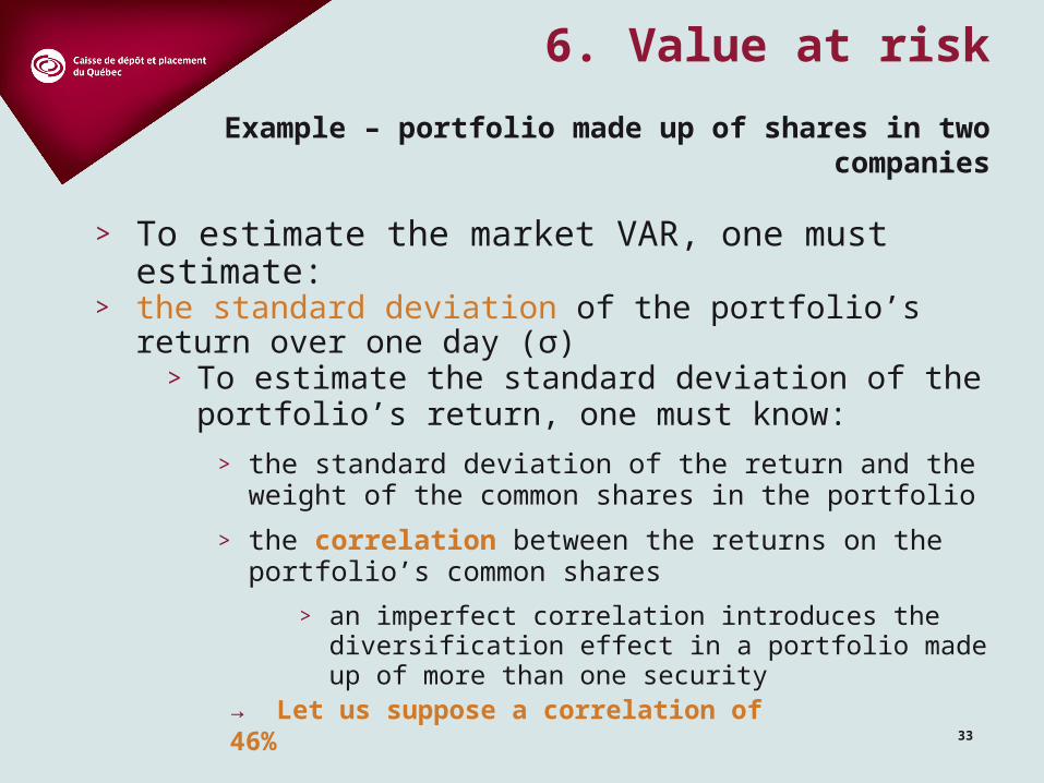
> To estimate the market VAR, one must estimate:> the standard deviation of the portfolio’s return over one day

(σ) > To estimate the standard deviation of the portfolio’s

return, one must know:

> the standard deviation of the return and the weight of the common shares in the portfolio

> the correlation between the returns on the portfolio’s common shares

> an imperfect correlation introduces the diversification effect in a portfolio made up of more than one security

6. Value at risk

→ Let us suppose a correlation of 46%

Example – portfolio made up of shares in two companies

34

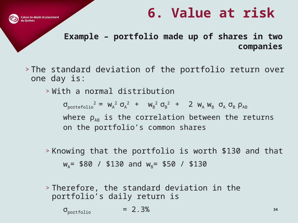
> The standard deviation of the portfolio return over one day is:

> With a normal distribution

σportefolio2 = wA

2 σA2 + wB

2 σB2 + 2 wA wB σA σB ρAB

where ρAB is the correlation between the returns on the portfolio’s common shares

> Knowing that the portfolio is worth $130 and that

wA= $80 / $130 and wB= $50 / $130

> Therefore, the standard deviation in the portfolio’s daily return is

σportfolio = 2.3%

6. Value at risk

Example – portfolio made up of shares in two companies

35

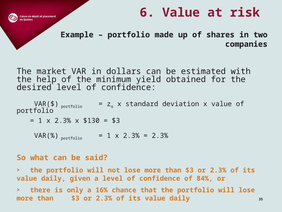
The market VAR in dollars can be estimated with the help of the minimum yield obtained for the desired level of confidence:

VAR($) portfolio = zα x standard deviation x value of portfolio

= 1 x 2.3% x $130 = $3

VAR(%) portfolio = 1 x 2.3% = 2.3%

So what can be said?

> the portfolio will not lose more than $3 or 2.3% of its value daily, given a level of confidence of 84%, or

> there is only a 16% chance that the portfolio will lose more than $3 or 2.3% of its value daily

6. Value at risk

Example – portfolio made up of shares in two companies

36

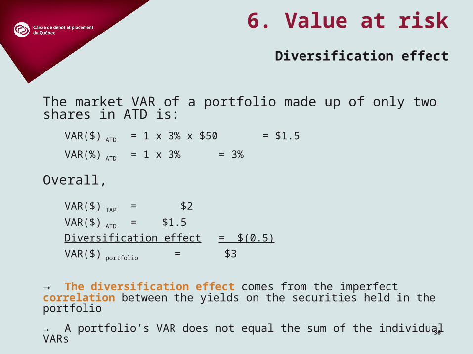
The market VAR of a portfolio made up of only two shares in ATD is:

VAR($) ATD = 1 x 3% x $50 = $1.5

VAR(%) ATD = 1 x 3% = 3%

Overall,

VAR($) TAP = $2

VAR($) ATD = $1.5

Diversification effect = $(0.5)

VAR($) portfolio = $3

→ The diversification effect comes from the imperfect correlation between the yields on the securities held in the portfolio

→ A portfolio’s VAR does not equal the sum of the individual VARs

6. Value at risk

Diversification effect