1

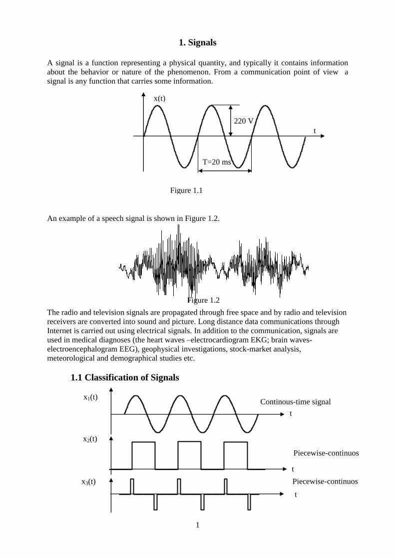
1. Signals

A signal is a function representing a physical quantity, and typically it contains information

about the behavior or nature of the phenomenon. From a communication point of view a

signal is any function that carries some information.

An example of a speech signal is shown in Figure 1.2.

The radio and television signals are propagated through free space and by radio and television

receivers are converted into sound and picture. Long distance data communications through

Internet is carried out using electrical signals. In addition to the communication, signals are

used in medical diagnoses (the heart waves –electrocardiogram EKG; brain waves-

electroencephalogram EEG), geophysical investigations, stock-market analysis,

meteorological and demographical studies etc.

1.1 Classification of Signals

Figure 1.2

220 V

T=20 ms

x(t)

t

Figure 1.1

Continous-time signal

Piecewise-continuos

Piecewise-continuos

x1(t)

x2(t)

x3(t)

t

t

t

2

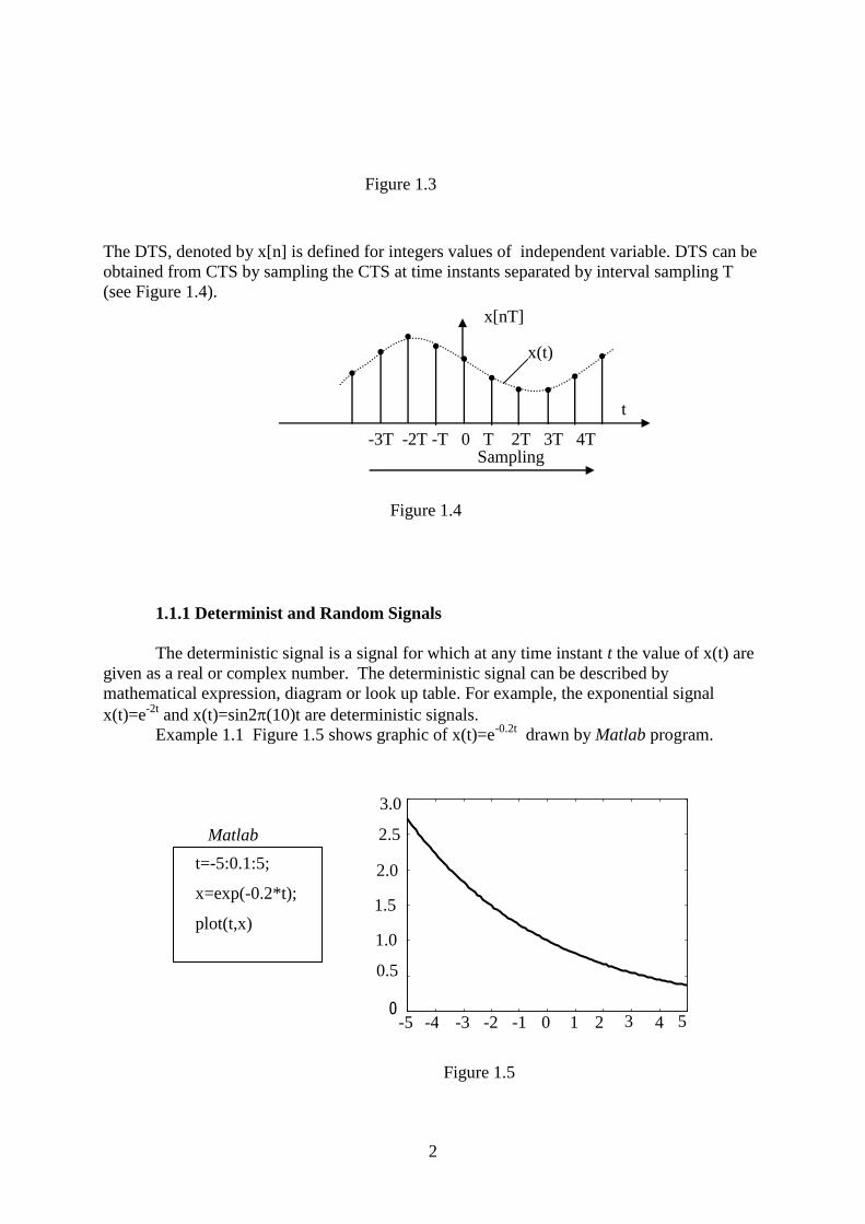
The DTS, denoted by x[n] is defined for integers values of independent variable. DTS can be

obtained from CTS by sampling the CTS at time instants separated by interval sampling T

(see Figure 1.4).

1.1.1 Determinist and Random Signals

The deterministic signal is a signal for which at any time instant t the value of x(t) are

given as a real or complex number. The deterministic signal can be described by

mathematical expression, diagram or look up table. For example, the exponential signal

x(t)=e-2t

and x(t)=sin2(10)t are deterministic signals.

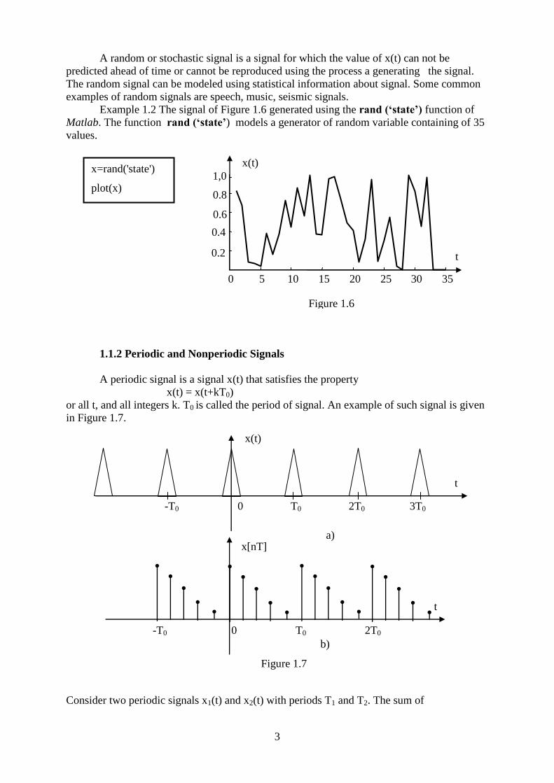
Example 1.1 Figure 1.5 shows graphic of x(t)=e-0.2t

drawn by Matlab program.

Matlab

Figure 1.3

x[nT]

t

-3T -2T -T 0 T 2T 3T 4T

Hr(j) =

a)

Hr(j) = Figure 1.4

x(t)

Sampling

5

3.0

2.5

2.0

1.5

0.5

1.0

0 4 3 2 1 0 -1 -2 -3 -4 -5

t=-5:0.1:5;

x=exp(-0.2*t);

plot(t,x)

Figure 1.5

3

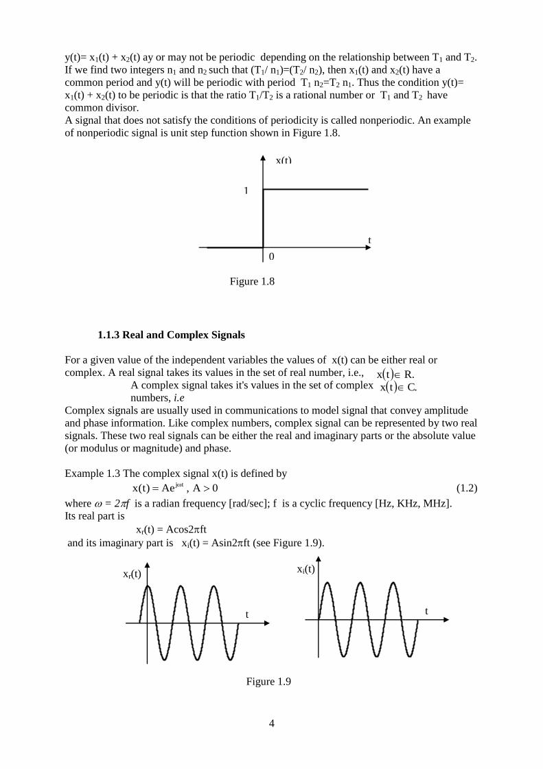
A random or stochastic signal is a signal for which the value of x(t) can not be

predicted ahead of time or cannot be reproduced using the process a generating the signal.

The random signal can be modeled using statistical information about signal. Some common

examples of random signals are speech, music, seismic signals.

Example 1.2 The signal of Figure 1.6 generated using the rand (‘state’) function of

Matlab. The function rand (‘state’) models a generator of random variable containing of 35

values.

1.1.2 Periodic and Nonperiodic Signals

A periodic signal is a signal x(t) that satisfies the property

x(t) = x(t+kT0)

or all t, and all integers k. T0 is called the period of signal. An example of such signal is given

in Figure 1.7.

Consider two periodic signals x1(t) and x2(t) with periods T1 and T2. The sum of

-T0 0 T0 2T0 3T0

x(t)

t

-T0 0 T0 2T0

x[nT]

t

Figure 1.7

a)

b)

x=rand('state')

plot(x)

Figure 1.6

0 5 10 15 20 25 30 35

0.2

0.4

0.6

0.8

1,0

t

x(t)

4

.Ctx

.Rtx

y(t)= x1(t) + x2(t) ay or may not be periodic depending on the relationship between T1 and T2.

If we find two integers n1 and n2 such that (T1/ n1)=(T2/ n2), then x1(t) and x2(t) have a

common period and y(t) will be periodic with period T1 n2=T2 n1. Thus the condition y(t)=

x1(t) + x2(t) to be periodic is that the ratio T1/T2 is a rational number or T1 and T2 have

common divisor.

A signal that does not satisfy the conditions of periodicity is called nonperiodic. An example

of nonperiodic signal is unit step function shown in Figure 1.8.

1.1.3 Real and Complex Signals

For a given value of the independent variables the values of x(t) can be either real or

complex. A real signal takes its values in the set of real number, i.e.,

A complex signal takes it's values in the set of complex

numbers, i.e

Complex signals are usually used in communications to model signal that convey amplitude

and phase information. Like complex numbers, complex signal can be represented by two real

signals. These two real signals can be either the real and imaginary parts or the absolute value

(or modulus or magnitude) and phase.

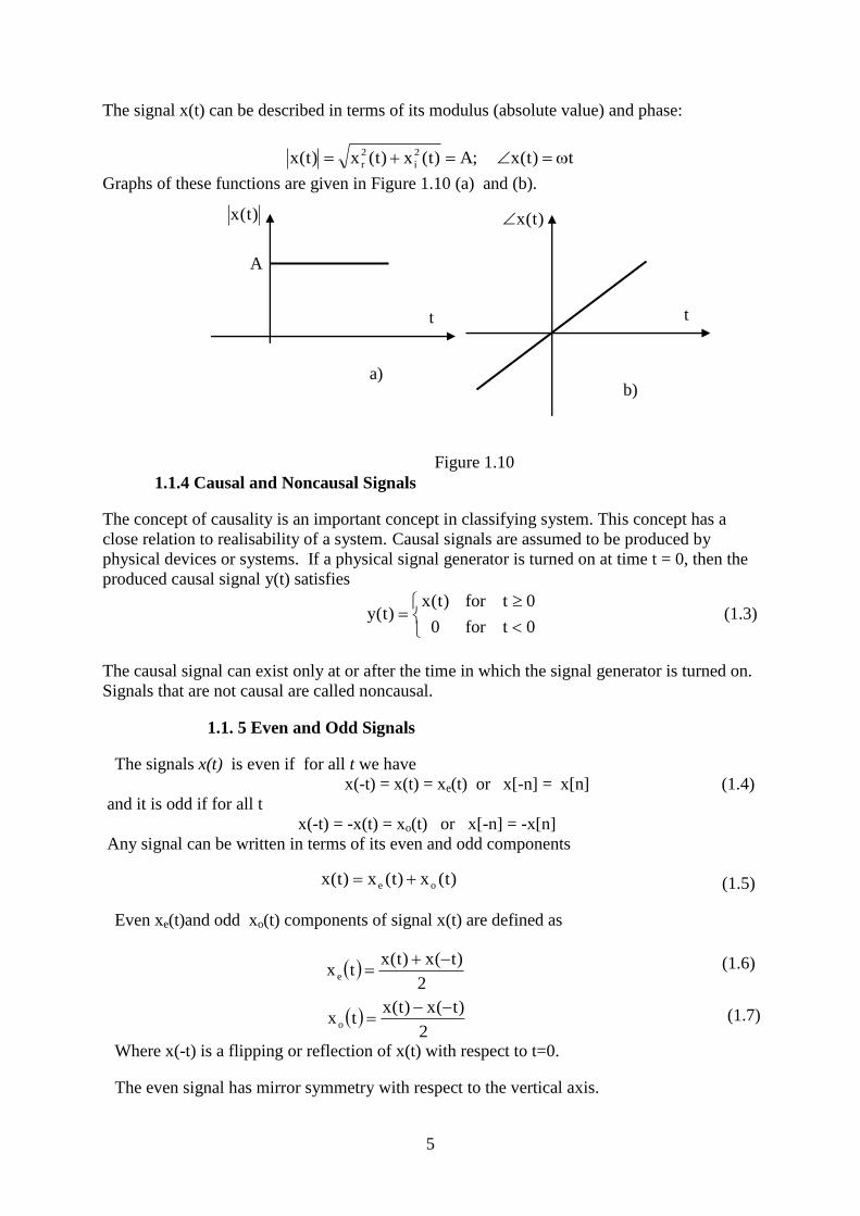
Example 1.3 The complex signal x(t) is defined by

0A,Ae)t(x tj (1.2)

where = 2f is a radian frequency [rad/sec]; f is a cyclic frequency [Hz, KHz, MHz].

Its real part is

xr(t) = Acos2ft

and its imaginary part is xi(t) = Asin2ft (see Figure 1.9).

xr(t)

t

xi(t)

t

Figure 1.9

0

1

t

x(t)

Figure 1.8

5

The signal x(t) can be described in terms of its modulus (absolute value) and phase:

t)t(x;A)t(x)t(x)t(x 2

i

2

r

Graphs of these functions are given in Figure 1.10 (a) and (b).

1.1.4 Causal and Noncausal Signals

The concept of causality is an important concept in classifying system. This concept has a

close relation to realisability of a system. Causal signals are assumed to be produced by

physical devices or systems. If a physical signal generator is turned on at time t = 0, then the

produced causal signal y(t) satisfies

0tfor0

0tfor)t(x)t(y (1.3)

The causal signal can exist only at or after the time in which the signal generator is turned on.

Signals that are not causal are called noncausal.

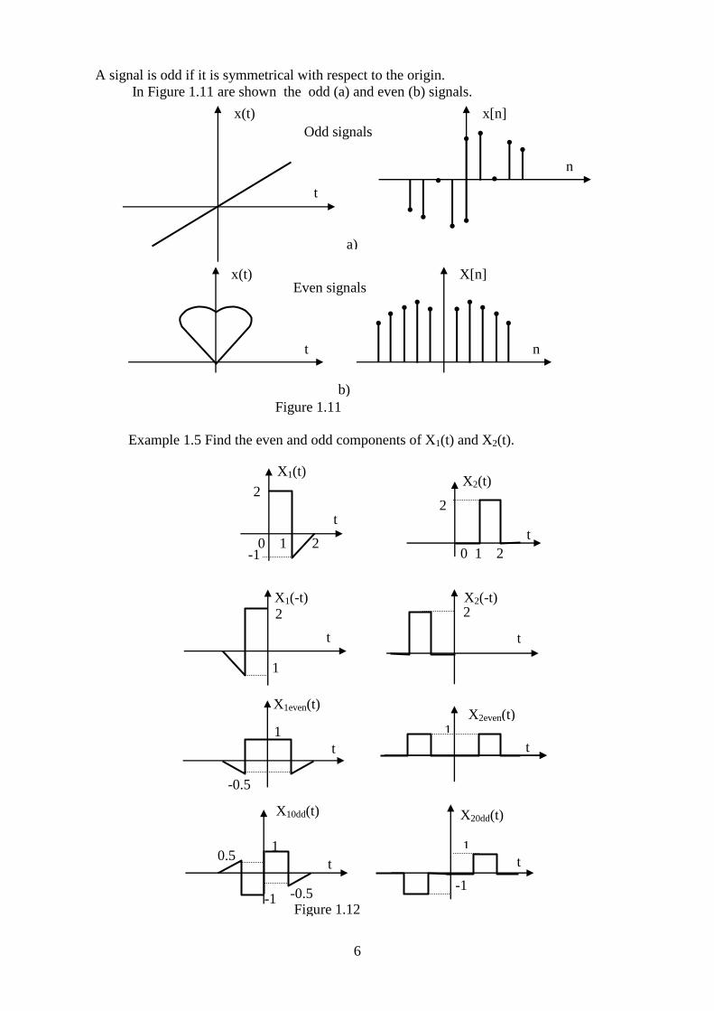
1.1. 5 Even and Odd Signals

The signals x(t) is even if for all t we have

x(-t) = x(t) = xe(t) or x[-n] = x[n] (1.4)

and it is odd if for all t

x(-t) = -x(t) = xo(t) or x[-n] = -x[n]

Any signal can be written in terms of its even and odd components

Even xe(t)and odd xo(t) components of signal x(t) are defined as

Where x(-t) is a flipping or reflection of x(t) with respect to t=0.

The even signal has mirror symmetry with respect to the vertical axis.

2

)t(x)t(xtx e

2

)t(x)t(xtx o

)t(x)t(x)t(x oe

)t(x

t t

A

)t(x

Figure 1.10

a) b)

(1.7)

(1.6)

(1.5)

6

t

x(t)

n

X[n]

A signal is odd if it is symmetrical with respect to the origin.

In Figure 1.11 are shown the odd (a) and even (b) signals.

Example 1.5 Find the even and odd components of X1(t) and X2(t).

Figure 1.12

Even signals

-1

X2(t)

0 1 2

t

X1(t)

0 1 2

t 2

2

X2even(t) X1even(t)

t t

1 1

-0.5

X2(-t) X1(-t)

t t

2 2

1

X10dd(t) X20dd(t)

t t

-1

1 1

-1 -0.5

0.5

Figure 1.11

b)

t

x(t)

n

x[n]

a)

Odd signals

7

1. 1. 6 Energy and Power types Signals

If v(t) and i(t) are respectively, the voltage and current across a resistor with resistance

R=1 resstor, then the instantaneous power is

The average energy expended over the time interval t1-t2=T

2t t 1t

2t

1t

2

2t

1t

dt)t(vT

1dt)t(p

T

1 =xE

For any signal x(t), the energy Ex is defned as

dt)t(xdt)t(xlimE2

T

T

2

Tx

The power xP of signal is

T

T

2

Tx dt)t(xT

1limP

For real signals )t(x)t(x 22 .

The signal x(t) is energy-type signal if and only if Ex well defined and finite 0<Ex>. For

power-type signals 0<Px>.

1.2 BASIC CONTINUOUS-TIME SIGNALS

In our study of communication systems, certain signals appear frequently. Here we

briefly introduce these signals and give some of their properties.

a) Exponential signal

The continuous time complex exponential signal is of the form

atCe)t(x

(1.10)

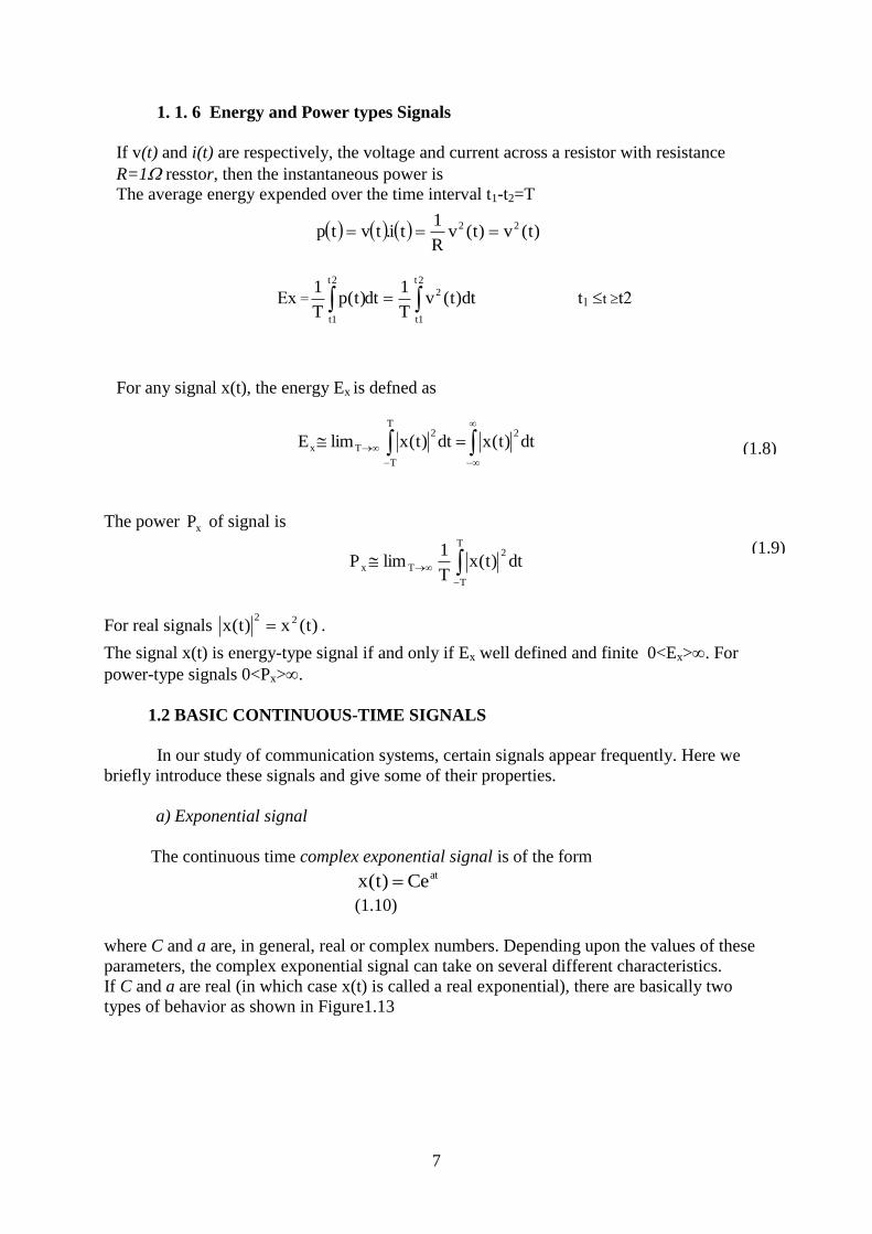
where C and a are, in general, real or complex numbers. Depending upon the values of these

parameters, the complex exponential signal can take on several different characteristics.

If C and a are real (in which case x(t) is called a real exponential), there are basically two

types of behavior as shown in Figure1.13

)t(v)t(vR

1ti.tvtp 22

(1.9)

(1.8)

8

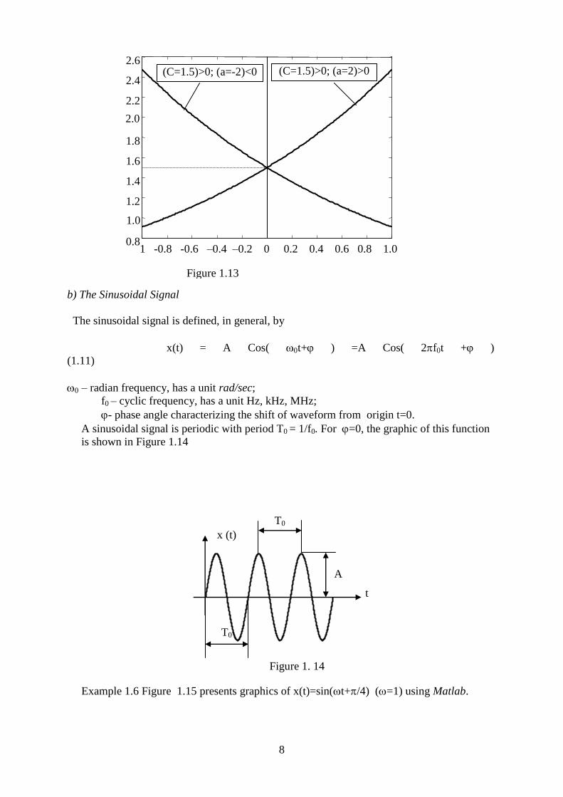
b) The Sinusoidal Signal

The sinusoidal signal is defined, in general, by

x(t) = A Cos( 0t+ ) =A Cos( 2f0t + )

(1.11)

0 – radian frequency, has a unit rad/sec;

f0 – cyclic frequency, has a unit Hz, kHz, MHz;

- phase angle characterizing the shift of waveform from origin t=0.

A sinusoidal signal is periodic with period T0 = 1/f0. For =0, the graphic of this function

is shown in Figure 1.14

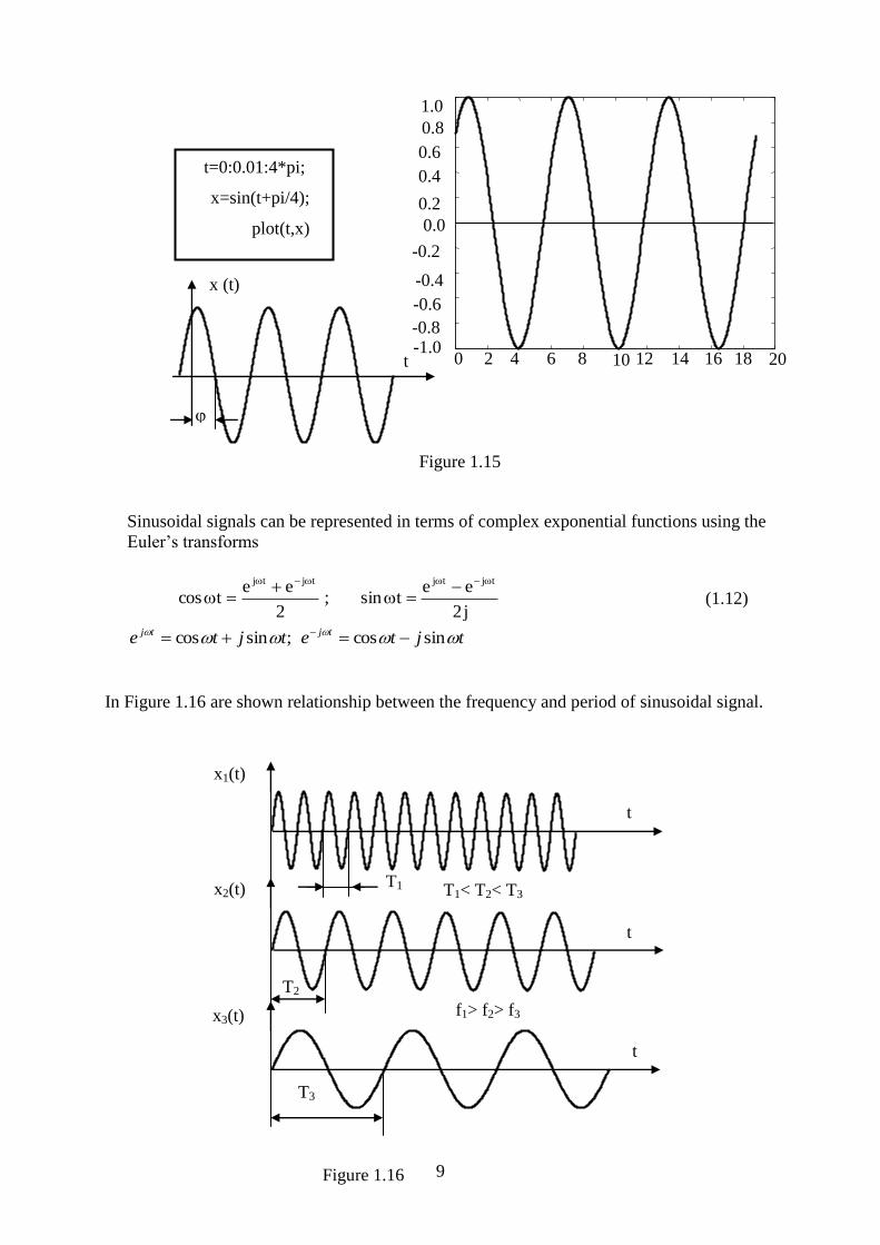
Example 1.6 Figure 1.15 presents graphics of x(t)=sin(t+/4) (=1) using Matlab.

0.8

1.0

1.2

1.4

1.6

1.8

2.0

2.2

2.4

2.6

1 -0.8 -0.6 –0.4 –0.2 0 0.2 0.4 0.6 0.8 1.0

(C=1.5)>0; (a=-2)<0 (C=1.5)>0; (a=2)>0

Figure 1.13

T0

T0

A

x (t)

t

Figure 1. 14

9

Figure 1.15

Sinusoidal signals can be represented in terms of complex exponential functions using the

Euler’s transforms

j2

eetsin;

2

eetcos

tjtjtjtj

tjtetjte tjtj sincos;sincos

In Figure 1.16 are shown relationship between the frequency and period of sinusoidal signal.

t=0:0.01:4*pi;

x=sin(t+pi/4);

plot(t,x)

2 4 6

0.0

-0.6

-0.4

0.2

0.4

0.6

0.8

1.0

-0.2

-0.8 -1.0

8 10

0

12

0

14

0

16

0

18

0 20 0

x (t)

t

x1(t)

x2(t)

x3(t)

T1

T2

T3

t

t

t

T1< T2< T3

f1> f2> f3

Figure 1.16

(1.12)

10

dt

)t(dU)t(

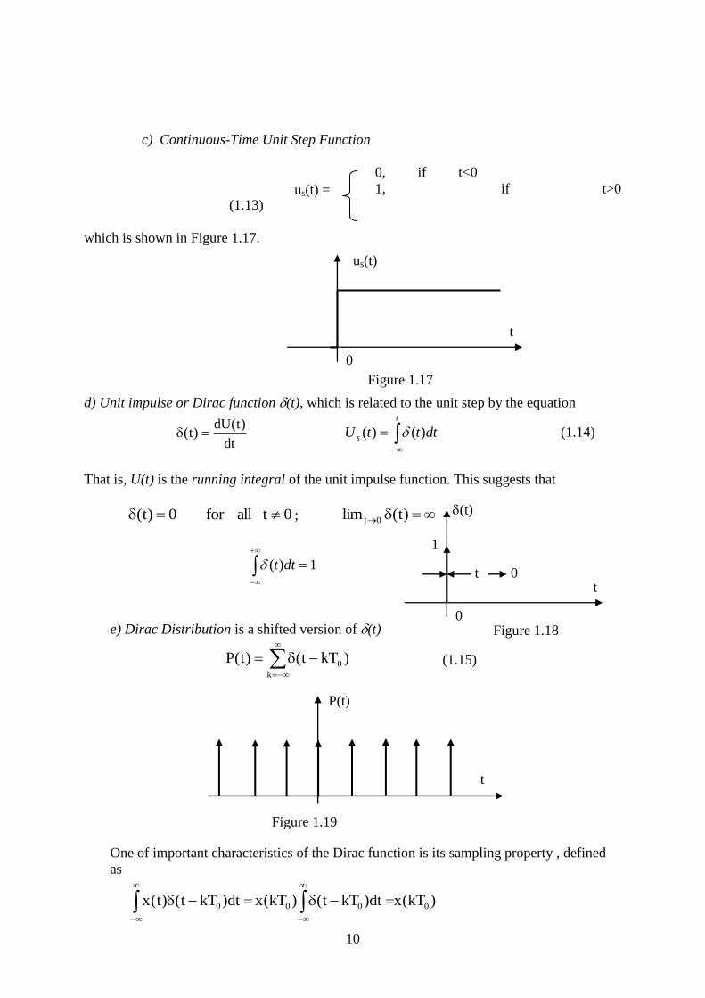
c) Continuous-Time Unit Step Function

0, if t<0

1, if t>0

(1.13)

which is shown in Figure 1.17.

d) Unit impulse or Dirac function (t), which is related to the unit step by the equation

t

s dtttU )()( (1.14)

That is, U(t) is the running integral of the unit impulse function. This suggests that

0tallfor0)t( ; )t(lim 0t

1)(

dtt

e) Dirac Distribution is a shifted version of (t)

k

0 )kTt()t(P (1.15)

One of important characteristics of the Dirac function is its sampling property , defined

as

us(t) =

t

us(t)

0

Figure 1.17

(t)

t

0

1

t 0

Figure 1.18

t

Figure 1.19

P(t)

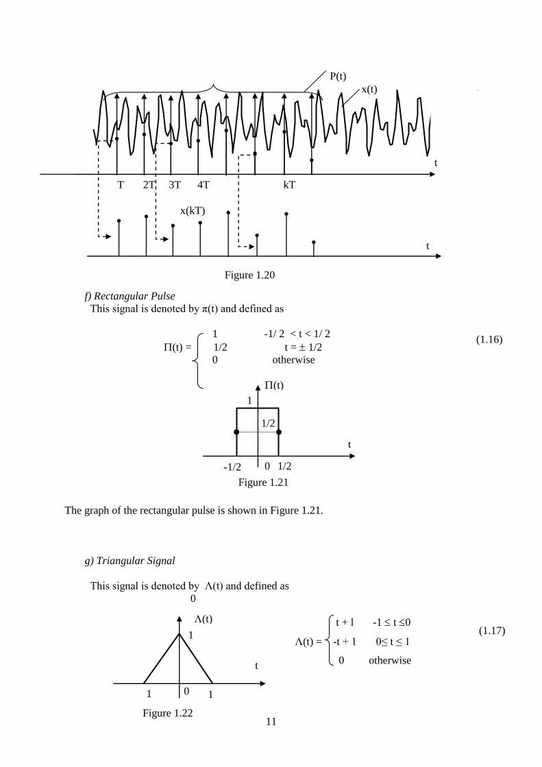
)kT(xdt)kTt()kT(xdt)kTt()t(x 0000

11

t

0

(t)

=

1 1

1

Figure 1.22

f) Rectangular Pulse

This signal is denoted by π(t) and defined as

1 -1/ 2 < t < 1/ 2

(t) = 1/2 t = 1/2

0 otherwise

The graph of the rectangular pulse is shown in Figure 1.21.

g) Triangular Signal

This signal is denoted by Λ(t) and defined as

0

t

0

(t)

=

-1/2 1/2

1/2

1

P(t)

t

t

x(t)

x(kT)

T 2T 3T 4T kT

Figure 1.20

(1.16)

Figure 1.21

t + l -1 t 0

Λ(t) = -t + 1 0≤ t ≤ 1

0 otherwise

(1.17)

12

-6 -5 -4 -3-2 -1 0 1 2 3 4 5 6

t

Sinc(t) 1

t=-2*pi:0.05:2*pi;

s=sin(pi*t)./(pi*t);

plot(t,x)

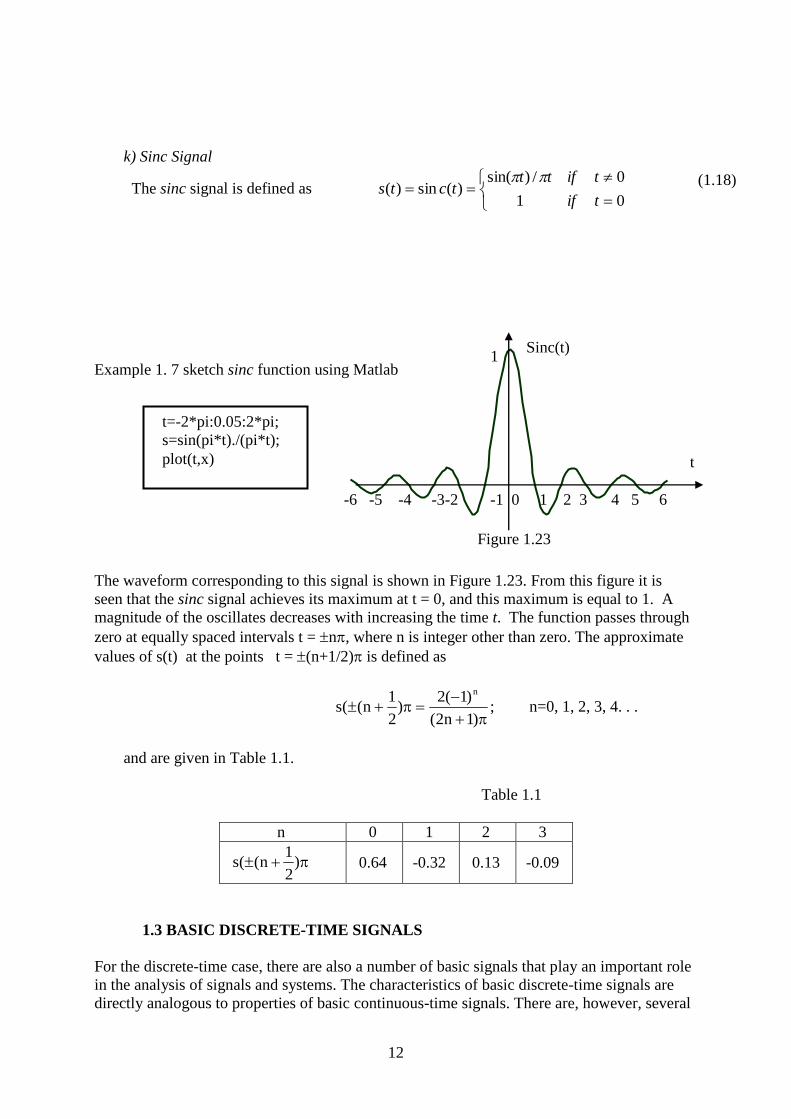
k) Sinc Signal

The sinc signal is defined as

01

0/)sin()(sin)(

tif

tiftttcts

Example 1. 7 sketch sinc function using Matlab

The waveform corresponding to this signal is shown in Figure 1.23. From this figure it is

seen that the sinc signal achieves its maximum at t = 0, and this maximum is equal to 1. A

magnitude of the oscillates decreases with increasing the time t. The function passes through

zero at equally spaced intervals t = n, where n is integer other than zero. The approximate

values of s(t) at the points t = (n+1/2) is defined as

;)1n2(

)1(2)

2

1n((s

n

n=0, 1, 2, 3, 4. . .

and are given in Table 1.1.

Table 1.1

n 0 1 2 3

)2

1n((s 0.64 -0.32 0.13 -0.09

1.3 BASIC DISCRETE-TIME SIGNALS

For the discrete-time case, there are also a number of basic signals that play an important role

in the analysis of signals and systems. The characteristics of basic discrete-time signals are

directly analogous to properties of basic continuous-time signals. There are, however, several

Figure 1.23

(1.18)

13

important differences in discrete time, and we will point these out as we examine the

properties of these signals.

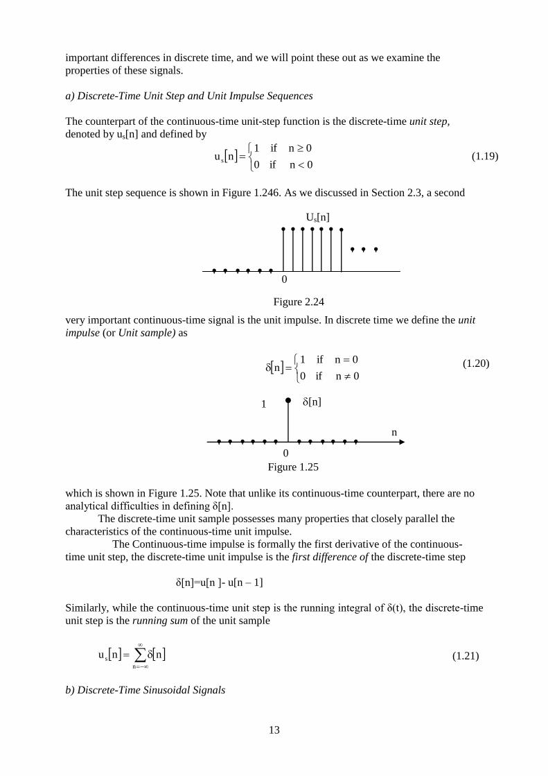
a) Discrete-Time Unit Step and Unit Impulse Sequences

The counterpart of the continuous-time unit-step function is the discrete-time unit step,

denoted by us[n] and defined by

0nif0

0nif1nu s

The unit step sequence is shown in Figure 1.246. As we discussed in Section 2.3, a second

very important continuous-time signal is the unit impulse. In discrete time we define the unit

impulse (or Unit sample) as

0nif0

0nif1n

which is shown in Figure 1.25. Note that unlike its continuous-time counterpart, there are no

analytical difficulties in defining δ[n].

The discrete-time unit sample possesses many properties that closely parallel the

characteristics of the continuous-time unit impulse.

The Continuous-time impulse is formally the first derivative of the continuous-

time unit step, the discrete-time unit impulse is the first difference of the discrete-time step

δ[n]=u[n ]- u[n – 1]

Similarly, while the continuous-time unit step is the running integral of δ(t), the discrete-time

unit step is the running sum of the unit sample

n

s nnu

b) Discrete-Time Sinusoidal Signals

Figure 2.24

Us[n]

0

(1.19)

(1.20)

(1.21)

0

[n]

n

Figure 1.25

1

14

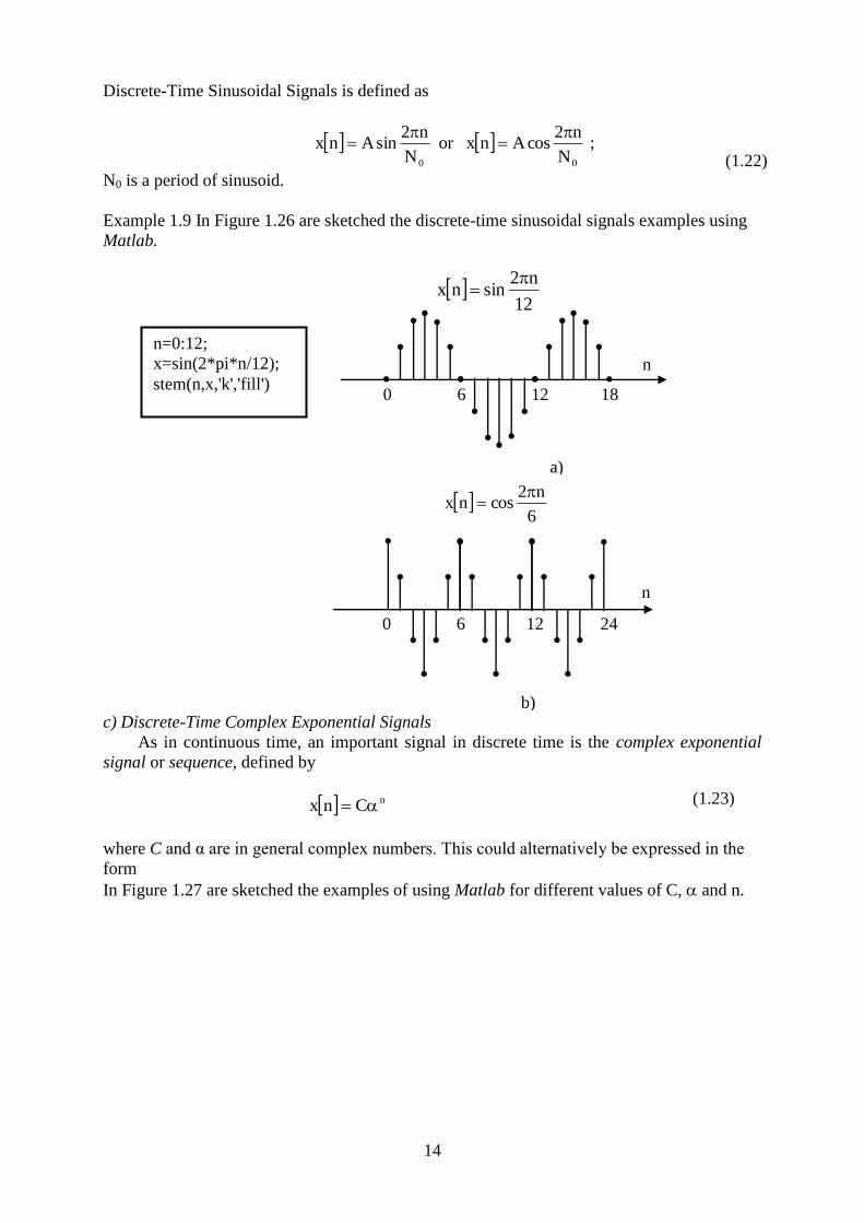
Discrete-Time Sinusoidal Signals is defined as

00 N

n2cosAnxor

N

n2sinAnx

;

N0 is a period of sinusoid.

Example 1.9 In Figure 1.26 are sketched the discrete-time sinusoidal signals examples using

Matlab.

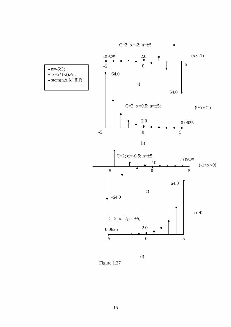
c) Discrete-Time Complex Exponential Signals

As in continuous time, an important signal in discrete time is the complex exponential

signal or sequence, defined by

nCnx

where C and α are in general complex numbers. This could alternatively be expressed in the

form

In Figure 1.27 are sketched the examples of using Matlab for different values of C, and n.

0 6 12 18

n

a)

12

n2sinnx

0 6 12 24

n

b)

6

n2cosnx

n=0:12;

x=sin(2*pi*n/12);

stem(n,x,'k','fill')

(1.22)

(1.23)

15

» n=-5:5;

» x=2*(-2).^n;

» stem(n,x,'k','fill')

C=2; =0.5; n=5;

Figure 1.27

C=2; =2; n=5;

>0

-64.0

-5 0 5

d)

64.0

2.0 0.0625

c)

2.0 -0.0625

-5 0 5

(-1<<0)

-5 0 5

b)

64.0

2.0 0.0625

(0<<1)

0 5 -5

-0.625

64.0

2.0 (<-1)

a)

C=2; =-2; n=5

C=2; =-0.5; n=5