1

Subjective Probability

Dr. Yan Liu

Department of Biomedical, Industrial and Human Factors EngineeringWright State University

2

Subjective Interpretation of Probability

Frequentist Interpretation of Probability Long-term frequency of occurrence of an event Requires repeatable experiments

Subjective interpretation of probability: an individual’s degree of belief in the occurrence of an event

What about the Following Events? Core meltdown of a nuclear reactor You being alive at the age of 80 Oregon beating Stanford in their 1970 football game (unsure about the outcome

although the event has happened)

3

Subjective Interpretation of Probability (Cont.)

Why Subjective Interpretation Frequentist interpretation is not always appropriate

Some events cannot be repeated many times e.g. Core meltdown of a nuclear power, your 80th birthday

The actual event has taken place, but you are uncertain about the result unless you have known the answer

e.g. The football game between Oregon and Stanford in 1970 Subjective interpretation allows us to model and structure individualistic

uncertainty through probability Degree of belief that a particular event will occur can vary among different people

and depend on the contexts

4

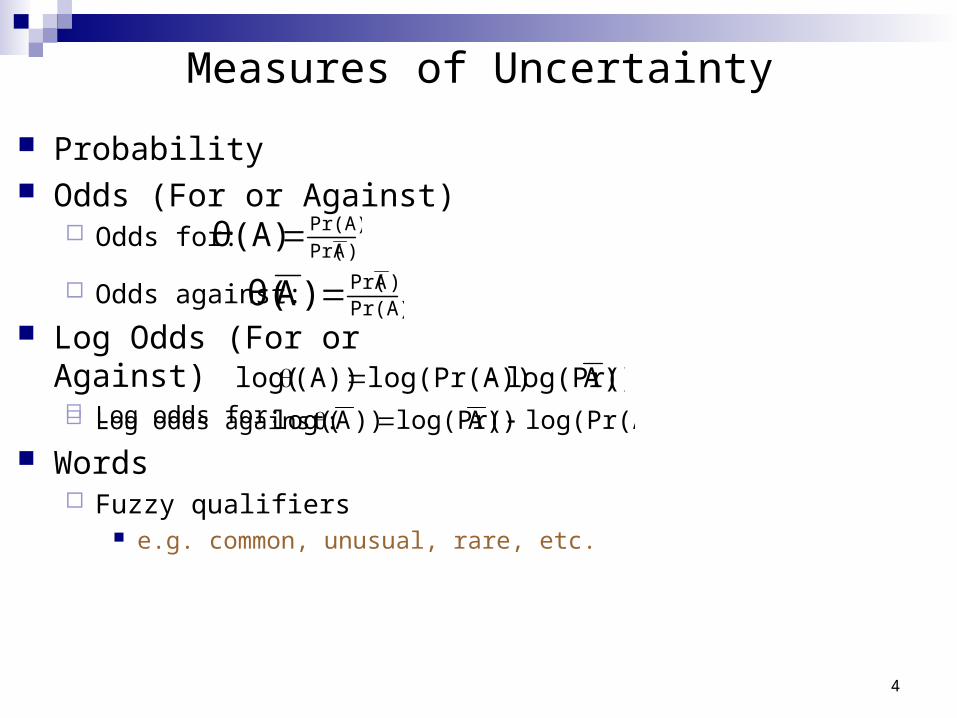
Measures of Uncertainty

Probability Odds (For or Against)

Odds for:)APr(

Pr(A)θ(A)

Pr(A))APr()Aθ(

))Alog(Pr(log(Pr(A))(A))log( log(Pr(A))))Alog(Pr())A(log(

Odds against:

Log Odds (For or Against) Log odds for:

Log odds against:

Words Fuzzy qualifiers

e.g. common, unusual, rare, etc.

5

Assessing Discrete Probabilities

Direct Methods Directly ask for probability assessment Simple to implement The decision maker may not be able to give a direct answer or place little

confidence in the answer Do not work well if the probabilities in questions are small

Indirect Methods Formulate questions in the decision maker’s domain of expertise and then

extract probability assessment through probability modeling Betting approach Reference lottery

6

Betting Approach

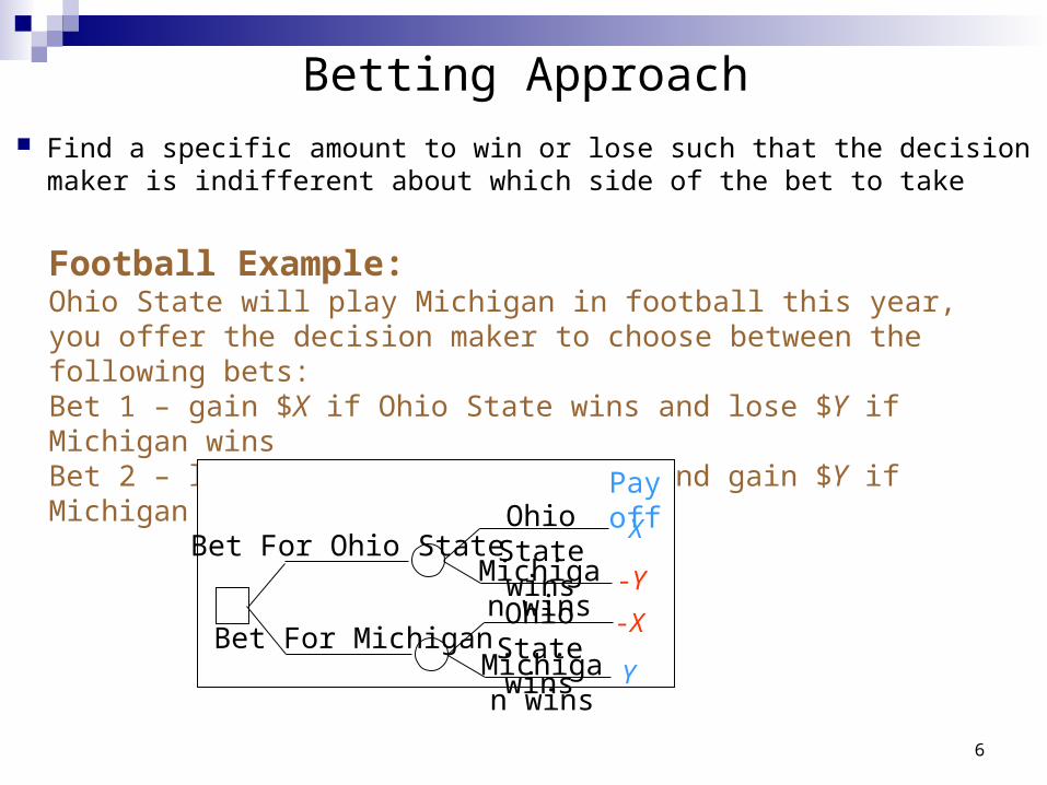
Find a specific amount to win or lose such that the decision maker is indifferent about which side of the bet to take

Football Example: Ohio State will play Michigan in football this year, you offer the decision maker to choose between the following bets: Bet 1 – gain $X if Ohio State wins and lose $Y if Michigan winsBet 2 – lose $X if Ohio State wins and gain $Y if Michigan wins

Bet For Ohio State

Bet For Michigan

Ohio State winsMichigan winsOhio State wins

Michigan wins

X

-Y

-X

Y

Payoff

7

Football Example (Cont.)

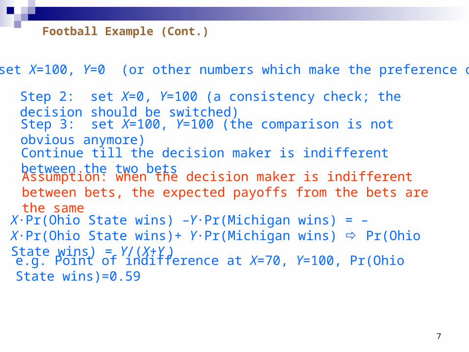
Step 1: set X=100, Y=0 (or other numbers which make the preference obvious)

Step 2: set X=0, Y=100 (a consistency check; the decision should be switched)

Step 3: set X=100, Y=100 (the comparison is not obvious anymore)

Continue till the decision maker is indifferent between the two bets

Assumption: when the decision maker is indifferent between bets, the expected payoffs from the bets are the same

X∙Pr(Ohio State wins) –Y∙Pr(Michigan wins) = –X∙Pr(Ohio State wins)+ Y∙Pr(Michigan wins) Pr(Ohio State wins) = Y/(X+Y )

e.g. Point of indifference at X=70, Y=100, Pr(Ohio State wins)=0.59

8

Betting Approach (Cont.)

Pro A straightforward approach

Cons Many people do not like the idea of betting Most people dislike the prospect of losing money (risk-averse) Does not allow choosing any other bets to protect from losses

9

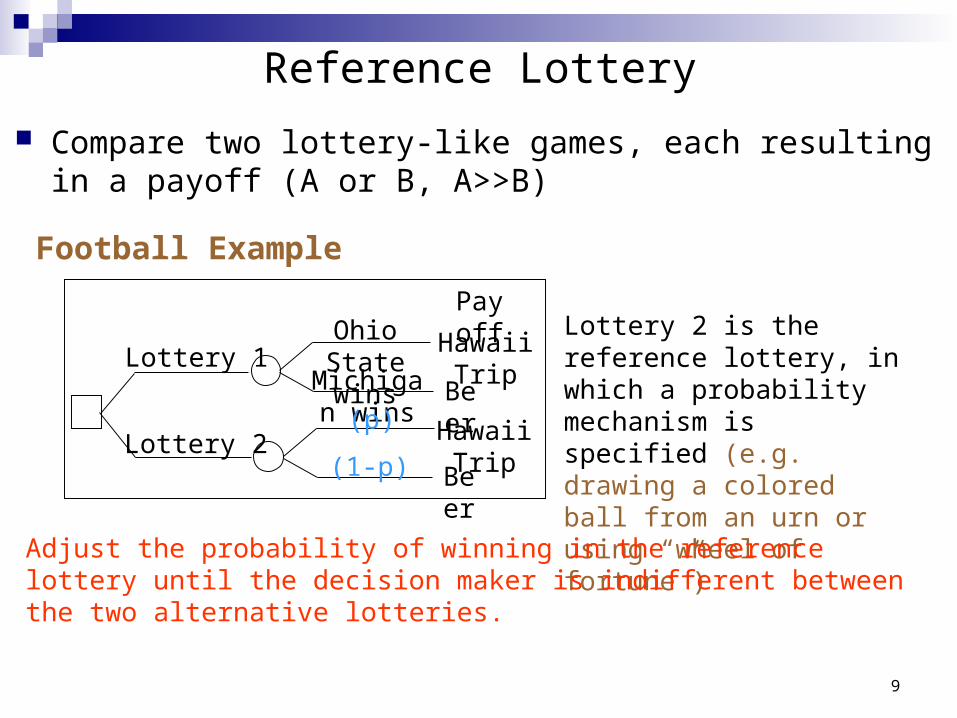
Reference Lottery

Lottery 1Ohio State

winsMichigan

wins(p)

(1-p)

Hawaii Trip

Beer

Payoff

Hawaii TripBe

er

Lottery 2

Lottery 2 is the reference lottery, in which a probability mechanism is specified (e.g. drawing a colored ball from an urn or using “wheel of fortune”)

Adjust the probability of winning in the reference lottery until the decision maker is indifferent between the two alternative lotteries.

Compare two lottery-like games, each resulting in a payoff (A or B, A>>B)

Football Example

10

Reference Lottery (Cont.)

Steps Step 1: Start with some p1 and ask which lottery the decision maker prefers Step 2: If lottery 1 is preferred, then choose p2 higher than p1; if the reference

lottery is preferred, then choose p2 less than p1 Continue till the decision maker is indifferent between the two lotteries

Assumption: when the decision maker is indifferent between lotteries, Pr(Ohio State wins)=p

Cons Some people have difficulties making assessments in hypothetical games Some people do not like the idea of a lottery-like game

11

Consistence and The Dutch Book

Subjective probabilities must follow the laws of probability. If they don’t, the person assessing the probabilities is inconsistent Dutch Book

A combination of bets which, on the basis of deductive logic, can be shown to entail a sure loss

Ohio State will play Michigan in football this year. Your friend says that Pr(Ohio State wins) = 40% and Pr(Michigan wins) = 50%. You note that the probabilities do not add up to 1, but your friend stubbornly refuses to change his estimates. You think, “Great! Let us set up two bets.”

Football Example:

12

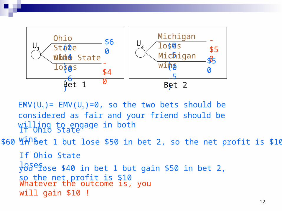
Ohio State wins(0.

4)Ohio State loses(0.

6)

$60-$40

Michigan loses(0.

5)Michigan wins(0.

5)

-$50$50

Bet 1 Bet 2

U1U2

EMV(U1)= EMV(U2)=0, so the two bets should be considered as fair and your friend should be willing to engage in both

If Ohio State wins,

you lose $40 in bet 1 but gain $50 in bet 2, so the net profit is $10

Whatever the outcome is, you will gain $10 !

you gain $60 in bet 1 but lose $50 in bet 2, so the net profit is $10

If Ohio State loses,

13

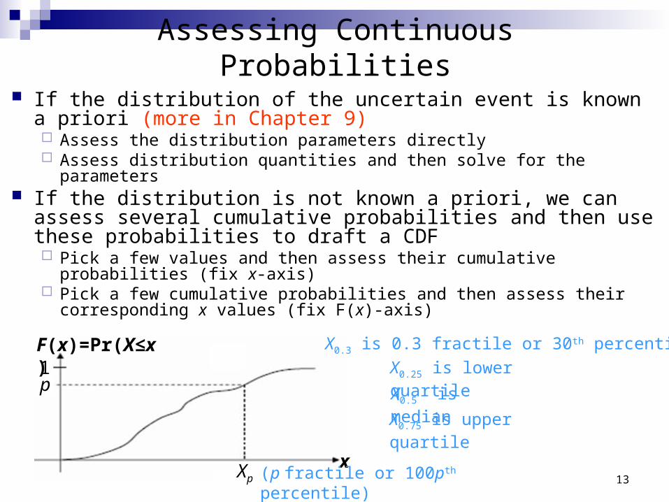
Assessing Continuous Probabilities

If the distribution of the uncertain event is known a priori (more in Chapter 9) Assess the distribution parameters directly Assess distribution quantities and then solve for the parameters

If the distribution is not known a priori, we can assess several cumulative probabilities and then use these probabilities to draft a CDF Pick a few values and then assess their cumulative probabilities (fix x-axis) Pick a few cumulative probabilities and then assess their corresponding x

values (fix F(x)-axis)

X0.25 is lower quartile

X0.5 is median

X0.75 is upper quartile

1p

Xpx

F(x)=Pr(X≤x)

(p fractile or 100pth percentile)

X0.3 is 0.3 fractile or 30th percentile

14

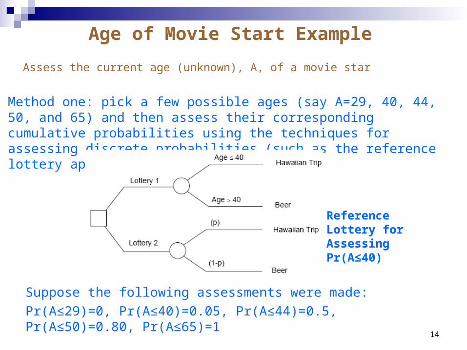
Assess the current age (unknown), A, of a movie star

Method one: pick a few possible ages (say A=29, 40, 44, 50, and 65) and then assess their corresponding cumulative probabilities using the techniques for assessing discrete probabilities (such as the reference lottery approach)

Suppose the following assessments were made:

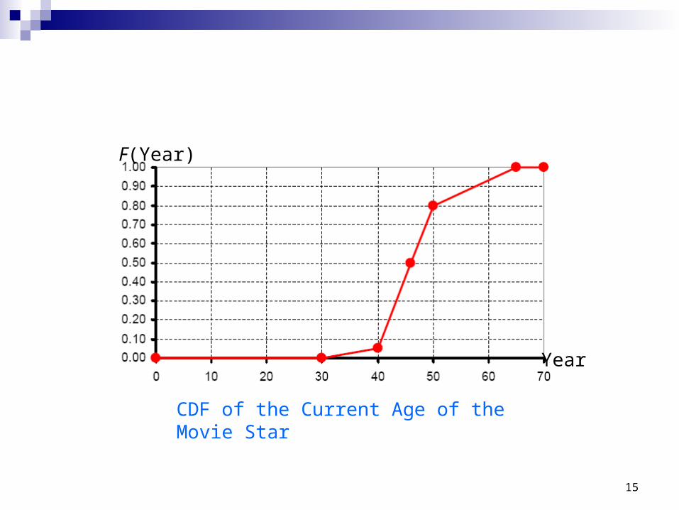
Pr(A≤29)=0, Pr(A≤40)=0.05, Pr(A≤44)=0.5, Pr(A≤50)=0.80, Pr(A≤65)=1

Reference Lottery for Assessing Pr(A≤40)

Age of Movie Start Example

15

Year

F(Year)

CDF of the Current Age of the Movie Star

16

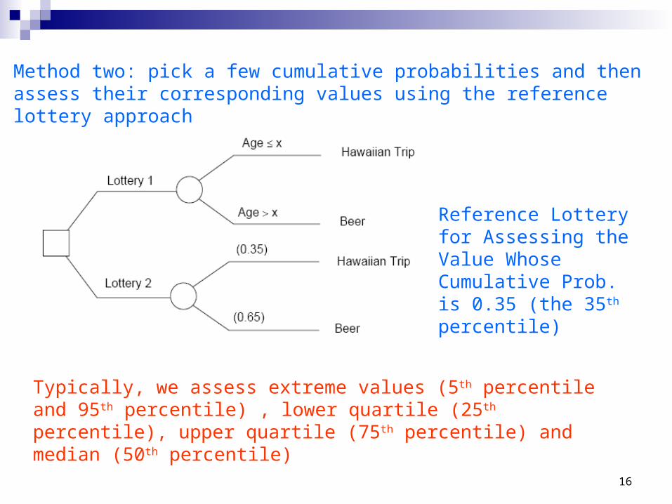
Method two: pick a few cumulative probabilities and then assess their corresponding values using the reference lottery approach

Typically, we assess extreme values (5th percentile and 95th percentile) , lower quartile (25th percentile), upper quartile (75th percentile) and median (50th percentile)

Reference Lottery for Assessing the Value Whose Cumulative Prob. is 0.35 (the 35th percentile)

17

Using Continuous CDF in Decision Trees

Monte Carlo Simulation (Not covered in this course; Chapter 11 of the textbook)

Approximate With a Discrete Distribution Use a few representative points in the distribution Extended Pearson – Tukey method Bracket median method

18

Extended Pearson-Tukey method

Uses the median, 5th percentile, and 95th percentile to approximate the continuous chance node, and their probabilities are 0.63, 0.185, and 0.185, respectively

Works the best for approximating symmetric distributions

19

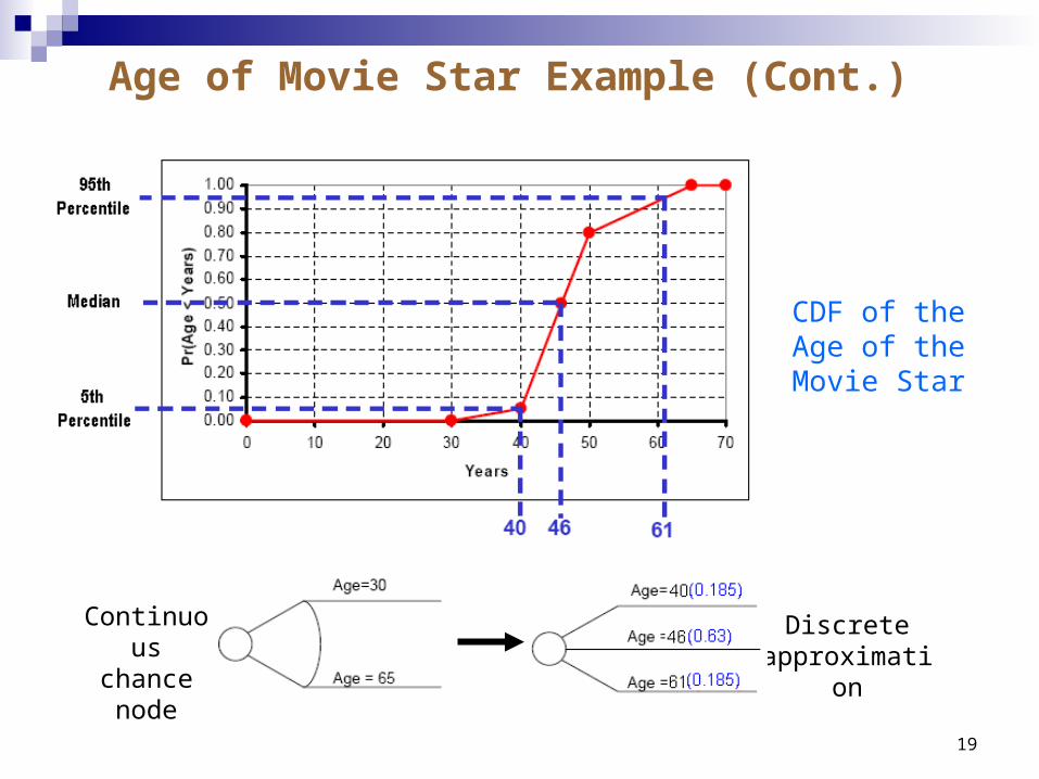
Continuous chance node

Discrete approximation

CDF of the Age of the Movie Star

Age of Movie Star Example (Cont.)

20

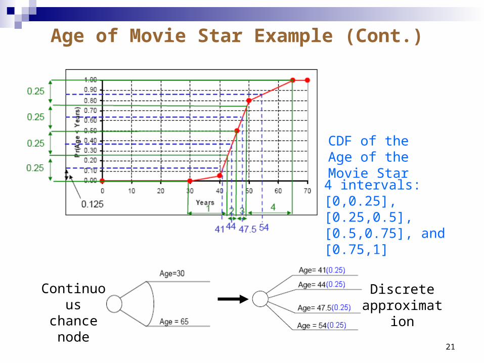
Bracket Median Method

The bracket median of interval [a,b] is a value m* between a and b such that Pr(a≤ X ≤ m*)=Pr(m*≤ X ≤ b)

Can approximate virtually any kind of distribution Steps

Step 1: Divide the entire range of probabilities into several equally likely intervals (typically three, four, or five intervals; the more intervals, the better the approximation yet more computations)

Step 2: Assess the bracket median for each interval Step 3: Assign equal probability to each bracket median (=100%/# of intervals )

21

Continuous chance node

Discrete approximation

4 intervals:[0,0.25],[0.25,0.5], [0.5,0.75], and [0.75,1]

CDF of the Age of the Movie Star

Age of Movie Star Example (Cont.)

22

Pitfalls: Heuristics and Biases

Thinking in terms of probability is NOT EASY! Heuristics

Rules of thumbs Simple and intuitively appealing May result in biases

Representative Bias Probability estimate is made on the basis of similarities within a group while

ignoring other relevant information (e.g. incidence/base rate) Insensitivity to the sample size (“Law of Small Numbers”)

Draw conclusions from highly representative yet small samples although small samples are subject to large statistical errors

What is the Law of Large Numbers ?

23

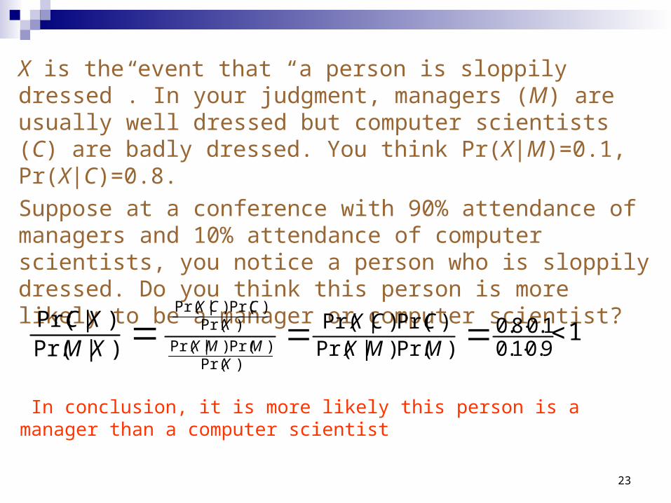
X is the event that “a person is sloppily dressed”. In your judgment, managers (M) are usually well dressed but computer scientists (C) are badly dressed. You think Pr(X|M)=0.1, Pr(X|C)=0.8.

Suppose at a conference with 90% attendance of managers and 10% attendance of computer scientists, you notice a person who is sloppily dressed. Do you think this person is more likely to be a manager or computer scientist?

9.01.01.08.0

)Pr()|Pr()Pr()|Pr(

)Pr()Pr()|Pr(

)Pr()Pr()|Pr(

MMX

CCX

XMMX

XCCX

In conclusion, it is more likely this person is a manager than a computer scientist

1)|Pr()|Pr(

XMXC

24

Pitfalls: Heuristics and Biases (Cont.)

Availability Bias Probability estimate is made according to the ease with which one can retrieve

similar events Illusory correlation

If two events are perceived as happening together frequently, this perception can lead to incorrect judgment regarding the strength of the relationship between the two events

Anchoring-and-Adjusting Bias Make an initial assessment(anchor) and then make subsequent assessments by

adjusting the anchor e.g. People make sales forecasting by considering the sales figures for the most

recent period and then adjusting those values based on new circumstances (usually insufficient adjustment)

Affects assessment of continuous probability distribution more often Motivational Bias

Incentives can lead people to report probabilities that do no entirely reflect their true beliefs

25

Expert and Probability Assessment

Experts Those knowledgeable about the subject matter

Protocol for Expert Assessment Identify the variables for which expert assessment is needed

Search for relevant scientific literature to establish scientific knowledge Identify and recruit experts

In-house expertise, external recruitment Motivate experts

Establish rapport and engender enthusiasm Structure and decompose

Develop a general model (e.g. influence diagram) to reflect relationships among variables

26

Expert and Probability Assessment

Protocols for Expert Assessment (Cont.) Probability assessment training

Explain the principles of probability assessment and provide opportunities of practice prior to the formal elicitation task

Probability elicitation and verification Make required probability assessments Check for consistency

Aggregate experts’ probability distribution

27

Expert Assessment Principles(Source: “Experts in Uncertainty” by Roger M. Cooke)

Reproducibility It must be possible for scientific peers to review and if necessary to reproduce

all calculations Calculation models must be fully specified and data must be made available

Accountability Source of expert judgment must be identified (their expertise levels and who

they work for) Empirical Control

Expert probability assessment must be susceptible to empirical control Neutrality

The method for combining/evaluating expert judgments should encourage experts to state true opinions

Fairness All experts are treated equally

28

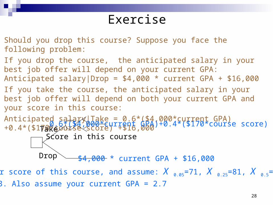
Exercise

Should you drop this course? Suppose you face the following problem:

If you drop the course, the anticipated salary in your best job offer will depend on your current GPA: Anticipated salary|Drop = $4,000 * current GPA + $16,000

If you take the course, the anticipated salary in your best job offer will depend on both your current GPA and your score in this course:

Anticipated salary|Take = 0.6*($4,000*current GPA)+0.4*($170*course score) +$16,000

Take

Drop

0.6*($4,000*current GPA)+0.4*($170*course score) +$16,000

$4,000 * current GPA + $16,000

Score in this course

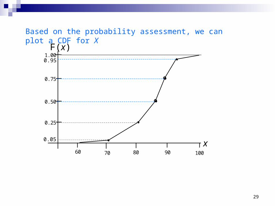
Let X = your score of this course, and assume: X 0.05=71, X 0.25=81, X 0.5=87, X 0.75=89,

and X 0.95=93. Also assume your current GPA = 2.7

29

Based on the probability assessment, we can plot a CDF for X

60 70 80 90 100

1.00

0.75

0.50

0.25

0.05

0.95

F(x)

x

30

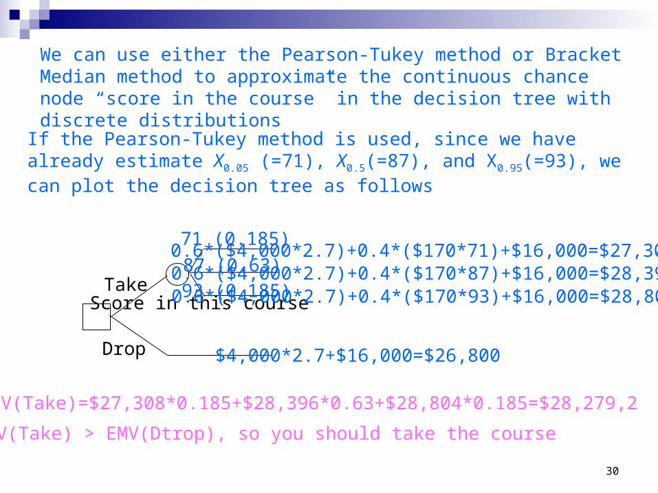
We can use either the Pearson-Tukey method or Bracket Median method to approximate the continuous chance node “score in the course” in the decision tree with discrete distributions

If the Pearson-Tukey method is used, since we have already estimate X0.05 (=71), X0.5(=87), and X0.95(=93), we can plot the decision tree as follows

Take

Drop $4,000*2.7+$16,000=$26,800

Score in this course

71 (0.185)

87 (0.63)93 (0.185)

0.6*($4,000*2.7)+0.4*($170*71)+$16,000=$27,3080.6*($4,000*2.7)+0.4*($170*87)+$16,000=$28,3960.6*($4,000*2.7)+0.4*($170*93)+$16,000=$28,804

EMV(Take)=$27,308*0.185+$28,396*0.63+$28,804*0.185=$28,279,2

EMV(Take) > EMV(Dtrop), so you should take the course

31

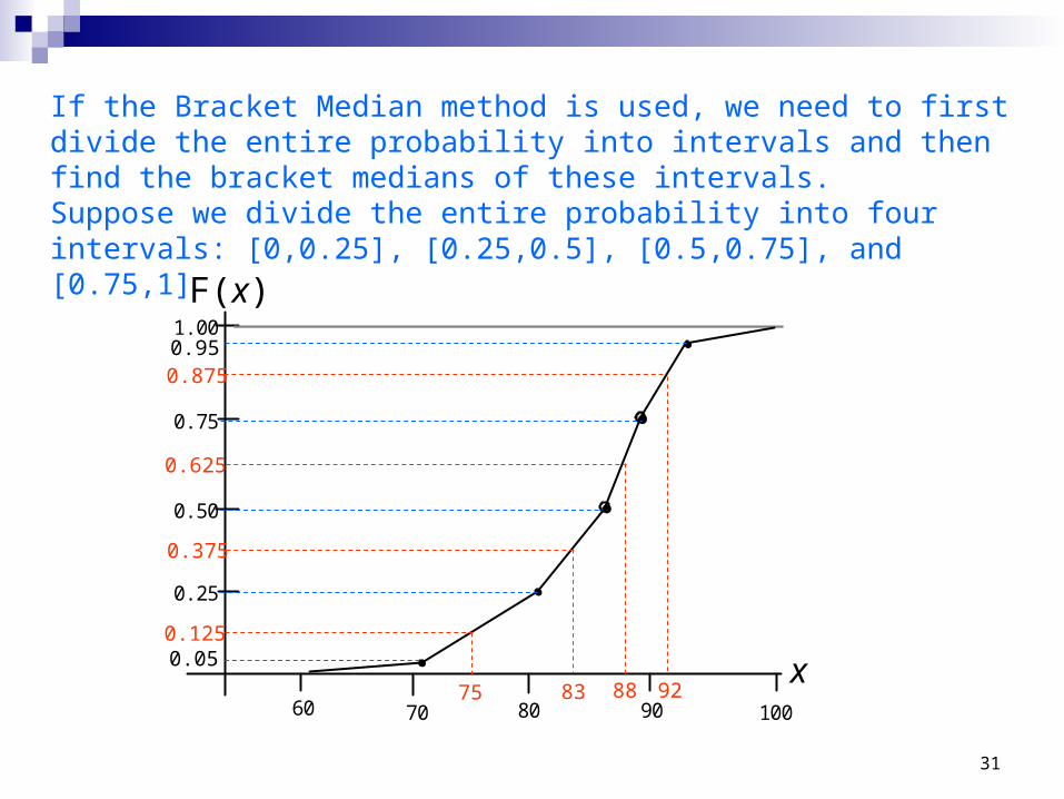
If the Bracket Median method is used, we need to first divide the entire probability into intervals and then find the bracket medians of these intervals. Suppose we divide the entire probability into four intervals: [0,0.25], [0.25,0.5], [0.5,0.75], and [0.75,1]

60 70 80 90 100

1.00

0.75

0.50

0.25

0.05

0.95

75 83 88 92

0.125

0.625

0.375

0.875

F(x)

x

32

Take

Drop $4,000*2.7+$16,000=$26,800

75 (0.25)83 (0.25)

88 (0.25)

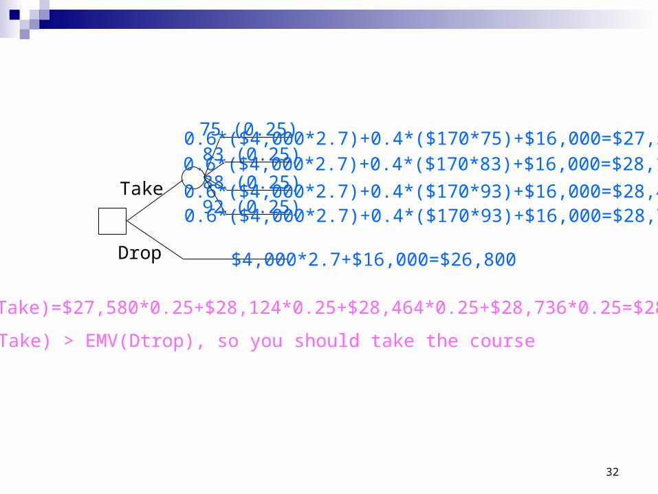
0.6*($4,000*2.7)+0.4*($170*75)+$16,000=$27,5800.6*($4,000*2.7)+0.4*($170*83)+$16,000=$28,124

0.6*($4,000*2.7)+0.4*($170*93)+$16,000=$28,46492 (0.25)0.6*($4,000*2.7)+0.4*($170*93)+$16,000=$28,736

EMV(Take)=$27,580*0.25+$28,124*0.25+$28,464*0.25+$28,736*0.25=$28,226

EMV(Take) > EMV(Dtrop), so you should take the course