10e 11 Chap Student Workbook - University of Daytonacademic.udayton.edu/MBA790/Student Workbook/10e_11_Chap_St… · this Workbook, you should be able to: Discuss three characteristics

Chapter 11: Managerial Decisions in Competitive Markets

220

Learning Objectives After reading Chapter 11 and working the problems for Chapter 11 in the textbook and in this Workbook, you should be able to:

Discuss three characteristics of perfectly competitive markets.

Apply the basic principles of marginal analysis to determine either (1) the profit-maximizing (or loss-minimizing) level of output, or (2) the profit-maximizing (or loss-minimizing) level of input usage.

Explain why the demand curve facing an individual firm in a perfectly competitive industry is perfectly elastic, and why this demand curve is also the marginal revenue curve for a competitive firm.

Explain why a firm should shut down in the short run if market price falls below minimum average variable cost.

Calculate profit margin (or average profit) and explain why profit margin should be ignored when making profit-maximizing decisions.

Explain why fixed costs are irrelevant to a manager’s production decision.

Define the concept of long-run competitive equilibrium and explain why a firm in long-run competitive equilibrium produces at the minimum point on long-run average cost.

Give a definition of increasing cost and constant cost industries and draw a long-run industry supply curve for a constant cost industry and for an increasing cost industry.

Explain, using the concept of economic rent, why it is possible for owners of exceptionally productive resources to “get rich” even though economic profit is zero in the long run for competitive markets.

Find the profit-maximizing (or loss-minimizing) level of output for a firm operating in a perfectly competitive market using empirical estimates (or forecasts) of (1) the market price of the commodity, (2) the average variable cost function, and (3) the marginal cost function.


221

Essential Concepts

1. Perfect competition occurs when a market possesses the following three charac-teristics:

i. Firms are price-takers because each firm produces only a very small portion of total market or industry output.

ii. All firms in the market produce a homogeneous or perfectly standardized product.

iii. Entry into and exit from the market is unrestricted. 2. The demand curve facing a competitive price-taking firm is horizontal or perfectly

elastic at the price determined by the intersection of the market demand and supply curves. Since marginal revenue equals price for a competitive firm, the demand curve is also simultaneously the marginal revenue curve (i.e., D = MR). Price-taking firms can sell all they want at the market price. Each additional unit of sales adds to total revenue an amount equal to price.

Profit Maximization in the Short Run: 3. In the short run, the firm incurs fixed costs that are unavoidable – i.e., they must be

paid even if output is zero—and variable costs that can be avoided if the firm chooses to shut down.

4. Shut down refers to the decision in the short run to produce zero output, which means the manager hires n variable inputs. The only costs incurred during shut down are the unavoidable fixed costs.

5. A manager makes two decisions in the short run: (1) whether to produce or shut down, and (2) if the decision is to produce, how much to produce.

6. In making the decision to produce or shut down, the manager will consider only the (avoidable) variable costs and will ignore fixed costs.

7. Profit margin is the difference between price and average total cost, which is equal to average profit (or profit per unit), as long as every unit is sold for the same price:

Average profit =πQ

=(P − ATC)Q

Q= P − ATC = Profit margin

8. The output level that maximizes profit margin is not the output level that maximizes profit. For this reason, managers should ignore profit margin or profit per unit when making their production decisions. See Figure 11.3 in the textbook for a numerical example that shows why it is a mistake to maximize profit margin.

9. Break-even points are the output levels – there are usually two of these points—where price equals average total cost, and thus profit equals zero at these points.


222

10. In the short run, the manager of a firm will choose to produce the output where P = SMC, rather than shut down, as long as total revenue is greater than or equal to the firm’s total avoidable cost or total variable cost (TR ≥ TVC ). Or, equivalently, a firm should produce as long as price is greater than or equal to average variable cost (P ≥ AVC ). If total revenue cannot cover total avoidable cost, that is, if total revenue is less than total variable cost (or equivalently, P < AVC), the manager will shut down and produce nothing, losing an amount equal to total fixed costs.

11. Fixed costs are irrelevant in the production decision because the level of fixed cost has no effect on either marginal cost or minimum average variable cost, and thus no effect on the optimal level of output.

12. Sunk costs are irrelevant in the production decision because such costs are forever unrecoverable, no matter what output decision is made, and so sunk costs cannot affect current or future decisions.

13. Average costs are also irrelevant for production decisions. Only marginal cost matters when finding the positive amount of output that maximizes profit. Technical note: AVC is not employed to find the optimal output, but rather to make sure the optimal output is not zero (i.e, whether to shut down or not).

14. Summary of the manager's output decision in the short-run:

i. Average variable cost tells whether to produce; the firm ceases to produce—shuts down—if price falls below minimum AVC.

ii. Marginal cost tells how much to produce; if P ≥ minimum AVC, the firm produces the output at which P = SMC.

iii. Average total cost tells how much profit or loss is made if the firm decides to produce; profit equals the difference between P and ATC multiplied by the quantity produced and sold.

15. The short-run supply curve for an individual price-taking firm is the portion of the firm’s marginal cost curve above minimum average variable cost. For market prices less than minimum average variable cost, quantity supplied is zero.

16. The short-run supply curve for a competitive industry can be obtained by horizon-tally summing the supply curves of all the individual firms in the industry. Short-run industry supply is always upward-sloping, and supply prices along the industry supply curve give the marginal costs of production for every firm contributing to industry supply.

17. Short-run producer surplus is the amount by which total revenue exceeds total variable cost and equals the area above the short-run supply curve below market price over the range of output supplied. Short-run producer surplus exceeds economic profit by the amount of total fixed costs.

Profit Maximization in the Long Run: 18. In long-run competitive equilibrium, all firms are in profit-maximizing equilibrium

(P = LMC). Long-run competitive equilibrium occurs because of the entry of new firms into the industry or the exit of existing firms from the industry. The market adjusts so that P = LMC = LAC, which is at the minimum point on LAC.


223

19. The long-run industry supply curve can be either flat (perfectly elastic) or upward sloping depending upon whether the industry is a constant cost industry or an increasing cost industry, respectively. a. For a constant cost industry, as industry output expands, input prices remain

constant, and the minimum point on LAC is unchanged. Since long-run supply price equals minimum LAC, the long-run industry supply curve is perfectly elastic (horizontal).

b. For an increasing cost industry, as industry output expands, input prices are bid up, causing the minimum point on LAC to rise, and long-run supply price to rise. The long-run industry supply curve for an increasing cost industry is upward sloping.

20. For both constant-cost and increasing-cost industries, long-run industry supply curves give supply prices for various levels of industry output allowing the industry to reach long-run competitive equilibrium. Thus, economic profit for every firm in the industry is zero at all points on the long-run industry supply. Furthermore, long-run supply prices give both LACmin and LMC for all firms in the industry.

21. Economic rent is a payment to the owner of a scarce, superior resource in excess of the resource’s opportunity cost. Firms that employ such exceptionally productive resources earn only a normal profit (economic profit is zero) in long-run competitive equilibrium because the potential economic profit from employing a superior resource is paid to the resource as rent.

22. As noted above, firms that employ exceptionally productive, superior resources earn zero economic profit in long-run competitive equilibrium. In increasing industries, all long-run producer surplus is paid to resource suppliers as economic rent. And, of course, for constant-cost industries there is zero producer surplus (and zero rent) since industry supply is perfectly horizontal.

Profit-Maximizing Input Usage: 23. Choosing either output or input usage to maximize profit leads to the same

maximum profit level. The profit-maximizing level of input usage produces exactly that level of output that maximizes profit. a. The marginal revenue product (MRP) of an additional unit of a variable

input is the additional revenue from hiring one more unit of the input. For the variable input labor:

TRMRP P MPL

Δ= = ×Δ

When a manager chooses to produce rather than shut down (TR > TVC), the optimal level of input usage is found by following this rule: If the marginal revenue product of an additional unit of the input is greater (less) than the price of the input, then that unit should (not) be hired. If the usage of the variable input varies continuously, the manager should employ the amount of the input at which MRP = input price.


224

b. Average revenue product (ARP) is the average revenue per worker (ARP = TR/L). ARP can be calculated as the product of price times the average product of labor:

TRARP P APL

= = ×

A manager should shut down operation in the short-run if there is no level of input usage for which ARP is greater than or equal to MRP. When ARP is less than MRP, total revenue is less than total variable cost, and the manager minimizes losses in the short run by shutting down.

Implementing the Profit-Maximizing Output Decision: 24. The following steps that use empirical estimates of price and costs can be

employed to find the profit-maximizing rate of production and the level of profit a competitive firm will earn. Step 1: Forecast the price of the product. Use the statistical techniques

presented in Chapter 7 to forecast the price of the product. Step 2: Estimate average variable cost (AVC) and marginal cost (SMC). The

cubic specification is the appropriate form for estimating a family of short-run cost curves:

2AVC a bQ cQ= + + and 22 3SMC a bQ cQ= + +

Step 3: Check the shutdown rule. If P ≥ AVCmin, then the manager should produce. If P < AVCmin, then the manager should shut down (i.e., Q* = 0).

Step 4: If P ≥ minAVC , find the output level where P = SMC. The profit-maximizing output level occurs where P = SMC. To find the optimal level of output, set forecasted price equal to estimated marginal cost and solve for Q*:

* *22 3P a bQ cQ= + +

Step 5: Compute profit or loss. Once a manager determines how much to produce, the calculation of total profit is a straightforward matter.

* *

*

Profit

( )

TR TCP Q AVC Q TFCP AVC Q TFC

= −= × − × −= − −

If minP AVC< , the firm shuts down, and profit is –TFC.


225

Matching Definitions average revenue product break-even points constant-cost industry economic rent increasing-cost industry long-run competitive equilibrium marginal revenue product perfect competition perfectly elastic demand profit margin (or average profit) quadratic formula shut down shutdown price

1. ___________________ A market structure in which a large number of firms sell a homogenous product or service with no restrictions on entry or exit and each firm is a price-taker.

2. ___________________ The demand facing a price-taking firm.

3. ___________________ A firm produces zero output but must still pay its fixed costs.

4. ___________________ Price minus average total cost.

5. ___________________ Output levels where P = ATC.

6. ___________________ Price below which a firm shuts down in the short run.

7. ___________________ All firms produce where price equals long-run marginal cost, and economic profits are zero.

8. ___________________ Industry in which input prices rise as all firms in the industry expand output.

9. ___________________ Industry in which input prices remain constant as all firms in the industry expand output.

10. ___________________ Payment in excess of a resource’s opportunity cost.

11. ___________________ The additional revenue earned by hiring one more unit of a variable input.

12 ___________________ The average revenue per worker.

13. ___________________ 2

1 24,

2B B ACX X

C− ± −=


226

Study Problems 1. The manager of a competitive firm will:

a. Produce rather than shut down if the forecasted price of the product is greater than ________.

b. Produce and make an economic profit if the forecasted price of the product is greater than ________.

c. Produce at a loss if the forecasted price is less than ________ but greater than ________.

d. Shut down if the forecasted price is less than ________. e. Minimize loss by producing the level of output where ________ equals

________ when forecasted price is greater than ________ but less than ________.

f. Maximize profit by producing the level of output where ________ equals ________ when forecasted price is greater than ________.

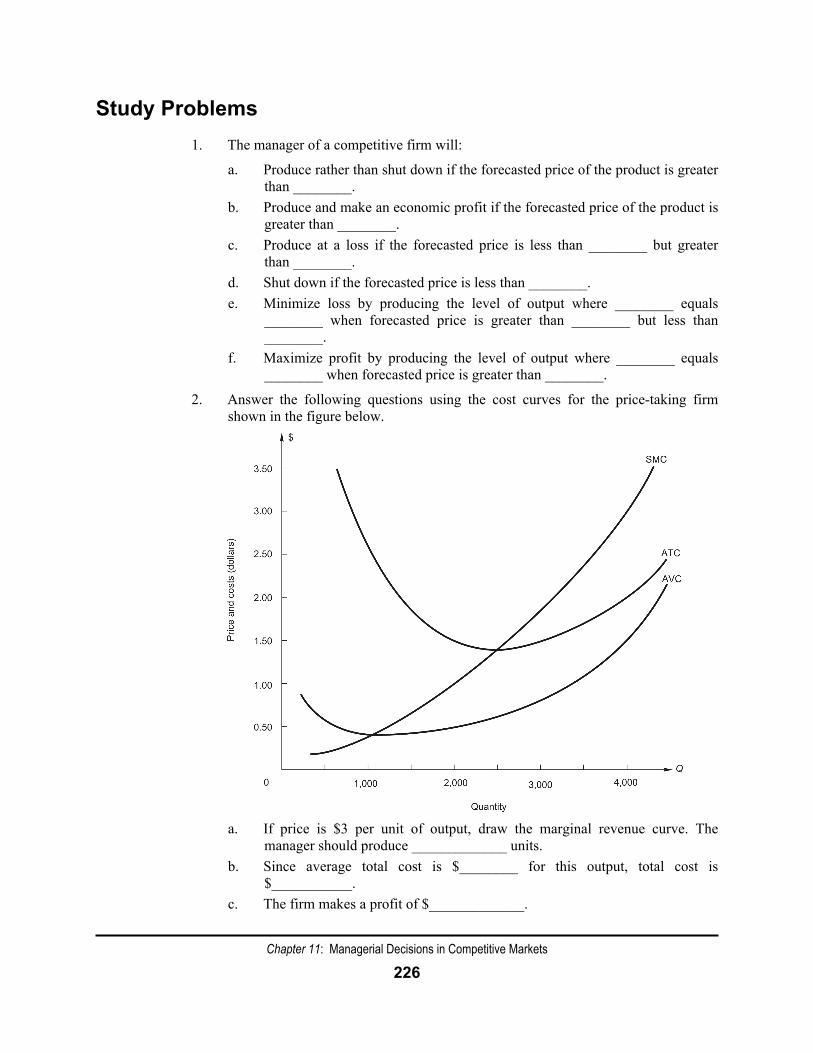
2. Answer the following questions using the cost curves for the price-taking firm shown in the figure below.

a. If price is $3 per unit of output, draw the marginal revenue curve. The

manager should produce _____________ units. b. Since average total cost is $________ for this output, total cost is

$___________. c. The firm makes a profit of $_____________.


227

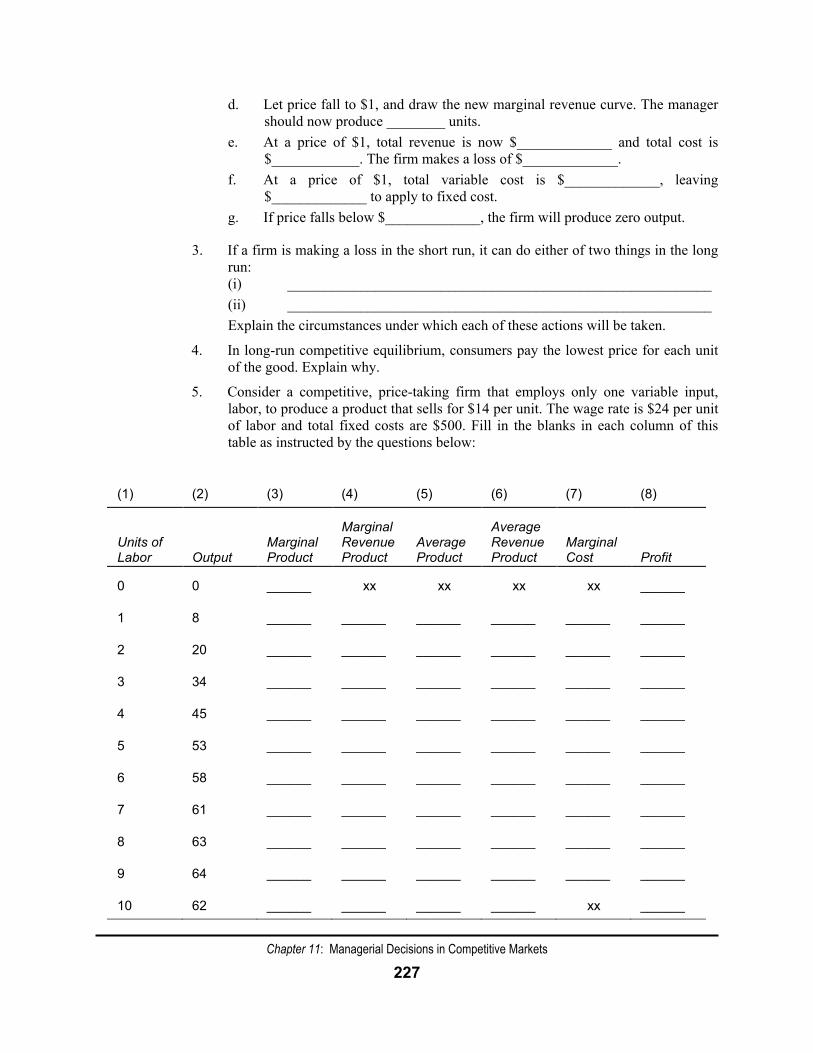
d. Let price fall to $1, and draw the new marginal revenue curve. The manager should now produce ________ units.

e. At a price of $1, total revenue is now $_____________ and total cost is $____________. The firm makes a loss of $_____________.

f. At a price of $1, total variable cost is $_____________, leaving $_____________ to apply to fixed cost.

g. If price falls below $_____________, the firm will produce zero output.

3. If a firm is making a loss in the short run, it can do either of two things in the long run: (i) __________________________________________________________ (ii) __________________________________________________________ Explain the circumstances under which each of these actions will be taken.

4. In long-run competitive equilibrium, consumers pay the lowest price for each unit of the good. Explain why.

5. Consider a competitive, price-taking firm that employs only one variable input, labor, to produce a product that sells for $14 per unit. The wage rate is $24 per unit of labor and total fixed costs are $500. Fill in the blanks in each column of this table as instructed by the questions below:

(1) (2) (3) (4) (5) (6) (7) (8)

Units of Labor

Output

Marginal Product

Marginal Revenue Product

Average Product

Average Revenue Product

Marginal Cost

Profit

0 0 ______ xx xx xx xx ______

1 8 ______ ______ ______ ______ ______ ______

2 20 ______ ______ ______ ______ ______ ______

3 34 ______ ______ ______ ______ ______ ______

4 45 ______ ______ ______ ______ ______ ______

5 53 ______ ______ ______ ______ ______ ______

6 58 ______ ______ ______ ______ ______ ______

7 61 ______ ______ ______ ______ ______ ______

8 63 ______ ______ ______ ______ ______ ______

9 64 ______ ______ ______ ______ ______ ______

10 62 ______ ______ ______ ______ xx ______


228

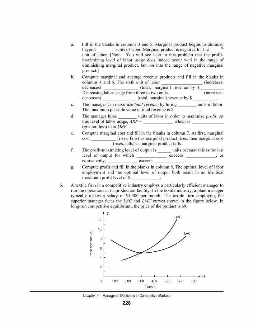
a. Fill in the blanks in columns 3 and 5. Marginal product begins to diminish beyond ________ units of labor. Marginal product is negative for the _____th unit of labor. [Note: You will see later in this problem that the profit-maximizing level of labor usage does indeed occur well in the range of diminishing marginal product, but not into the range of negative marginal product.]

b. Compute marginal and average revenue products and fill in the blanks in columns 4 and 6. The sixth unit of labor __________________ (increases, decreases) _______________ (total, marginal) revenue by $__________. Decreasing labor usage from three to two units _______________ (increases, decreases) _______________ (total, marginal) revenue by $___________.

c. The manager can maximize total revenue by hiring ________ units of labor. The maximum possible value of total revenue is $____________.

d. The manager hires ________ units of labor in order to maximize profit. At this level of labor usage, ARP = _____________ which is ______________ (greater, less) than MRP.

e. Compute marginal cost and fill in the blanks in column 7. At first, marginal cost ___________ (rises, falls) as marginal product rises, then marginal cost _____________ (rises, falls) as marginal product falls.

f. The profit-maximizing level of output is ______ units because this is the last level of output for which _____________ exceeds _____________, or equivalently, _____________ exceeds _____________ .

g. Compute profit and fill in the blanks in column 8. The optimal level of labor employment and the optimal level of output both result in an identical maximum profit level of $_____________.

6. A textile firm in a competitive industry employs a particularly efficient manager to run the operations at its production facility. In the textile industry, a plant manager typically makes a salary of $4,500 per month. The textile firm employing the superior manager faces the LAC and LMC curves shown in the figure below. In long-run competitive equilibrium, the price of the product is $9.


229

a. A typical textile firm in this competitive industry has a minimum long-run average cost of $______. The typical textile firm earns economic profit of $______.

b. The textile firm with the superior plant manager could earn economic profit of $___________ per month, if no rent is paid to the superior manager.

c. The superior plant manager is likely to earn a salary of $______ per month, $____________ of which is economic rent.

d. If the superior plant manager also owned the textile firm, she would earn $___________ of economic profit. Explain your answer.

7. Consider a price-taking firm in the competitive industry for raw chocolate. The market demand and supply functions for raw chocolate are estimated to be

Chocolate demand: Q = 10,000 – 10,000P + 2M Chocolate supply: Q = 40,000 + 10,000P – 4,000PI

where Q is the number of 10 pound bars per month, P is the price of a 10 pound bar of raw chocolate, income is M, and PI is the price of cocoa (the primary ingredient input). The manager of ABC Cocoa Products uses time-series data to obtain the following forecasted values of M and PI for 2011:

M = $25,000 and PI = $10

The manager of ABC Cocoa also estimates its average variable cost function to be

AVC = 3.0 – 0.0027Q + 0.0000009Q2

Fixed costs at ABC will be $1,600 in 2011.

a. The price of raw chocolate in 2011 is forecasted to be $__________. b Average variable cost reaches its minimum value at __________ bars of

chocolate per month. c. The minimum value of average variable cost is $__________. d. Should ABC Cocoa produce or shut down? e. The marginal cost function for the firm is

SMC = _________________________________. f. The optimal level of production for the firm is __________ bars of chocolate

per month. g. The maximum profit (minimum loss) that ABC can expect to earn is

$__________. Next let forecasted price of raw chocolate fall to $1.50. h. The optimal level of production for ABC is now ________ bars of chocolate

per month. i. The profit (loss) for ABC is forecasted to be $________.


230

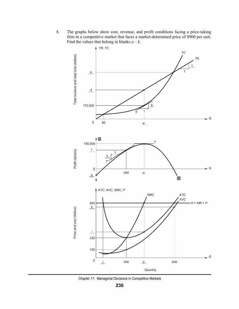
8. The graphs below show cost, revenue, and profit conditions facing a price-taking firm in a competitive market that faces a market-determined price of $900 per unit. Find the values that belong in blanks a – k.


231

9. Answer the following questions based on the figure and your answers in Study Problem 8.

a. What is average fixed cost at 250 units? At 650 units? What is total fixed cost at 250 units? At 650 units? Using these values, explain how AFC and TFC are related to increases in Q.

b. What are the two break-even values of output? In the top panel, construct a tangent line to TC at each one of the break-even points. At the lower break-even point, is the tangent line steeper or flatter than TR? In the bottom panel, should MR be greater or less than SMC at the lower break-even point? Explain. What happens at the higher output where break-even occurs?

c. Why is the slope of the profit function zero at the profit-maximizing level of output?

d. At what level of output is profit margin or average profit maximized? How much more profit can the firm earn by producing the output where MR = MC than by producing where unit costs are minimized?

e. When the manager is producing 400 units, the firm’s marketing director complains that the firm should increase output to 500 units because this will increase revenues by $90,000. If you were the manager of this firm, how would you respond to this advice?

Multiple Choice / True-False

1. Which of the following statements is not a characteristic of a perfectly competitive firm? a. Perfectly competitive firms view each other as fierce rivals. b. Firms are price-takers. c. All firms produce a homogeneous product. d. Perfectly competitive markets allow freedom of entry and exit.

2. Since the firm’s demand curve is perfectly elastic for a price-taking firm, a. P = MR. b. P = MRP. c. P = TR. d. both a and b. e. both a and c.

3. In the short run, a firm shuts down when a. profit is negative. b. TR < TVC. c. MRP > ARP at the level of labor usage where MRP = w. d. both b and c. e. all of the above.


232

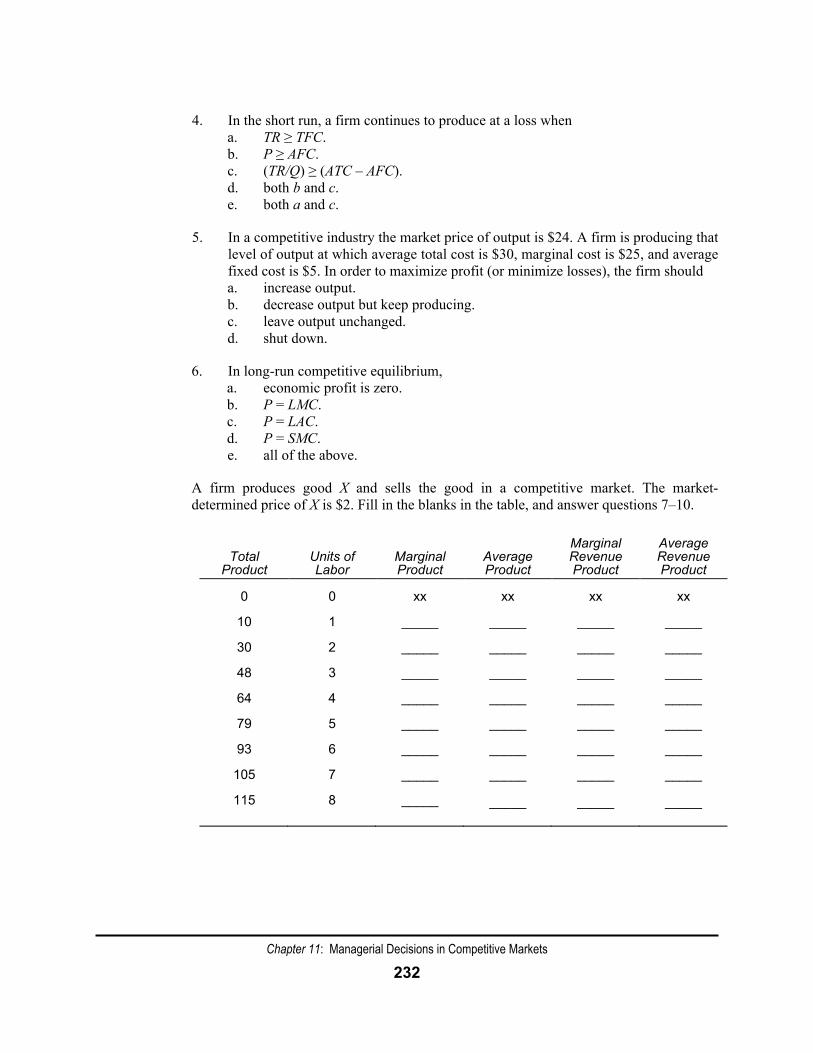
4. In the short run, a firm continues to produce at a loss when a. TR ≥ TFC. b. P ≥ AFC. c. (TR/Q) ≥ (ATC – AFC). d. both b and c. e. both a and c.

5. In a competitive industry the market price of output is $24. A firm is producing that level of output at which average total cost is $30, marginal cost is $25, and average fixed cost is $5. In order to maximize profit (or minimize losses), the firm should a. increase output. b. decrease output but keep producing. c. leave output unchanged. d. shut down.

6. In long-run competitive equilibrium, a. economic profit is zero. b. P = LMC. c. P = LAC. d. P = SMC. e. all of the above.

A firm produces good X and sells the good in a competitive market. The market-determined price of X is $2. Fill in the blanks in the table, and answer questions 7–10.

Total

Product

Units of Labor

Marginal Product

Average Product



0 0 xx xx xx xx

10 1 _____ _____ _____ _____

30 2 _____ _____ _____ _____

48 3 _____ _____ _____ _____

64 4 _____ _____ _____ _____

79 5 _____ _____ _____ _____

93 6 _____ _____ _____ _____

105 7 _____ _____ _____ _____

115 8 _____ _____

_____ _____


233

7. The marginal revenue product for the third unit of labor is ________. a. $18 b. $48 c. $16 d. $9 e. $36

8. At a wage rate of $22, the firm will hire a. 0 units of labor. b. 1 unit of labor. c. 3 units of labor. d. 7 units of labor. e. 8 units of labor.



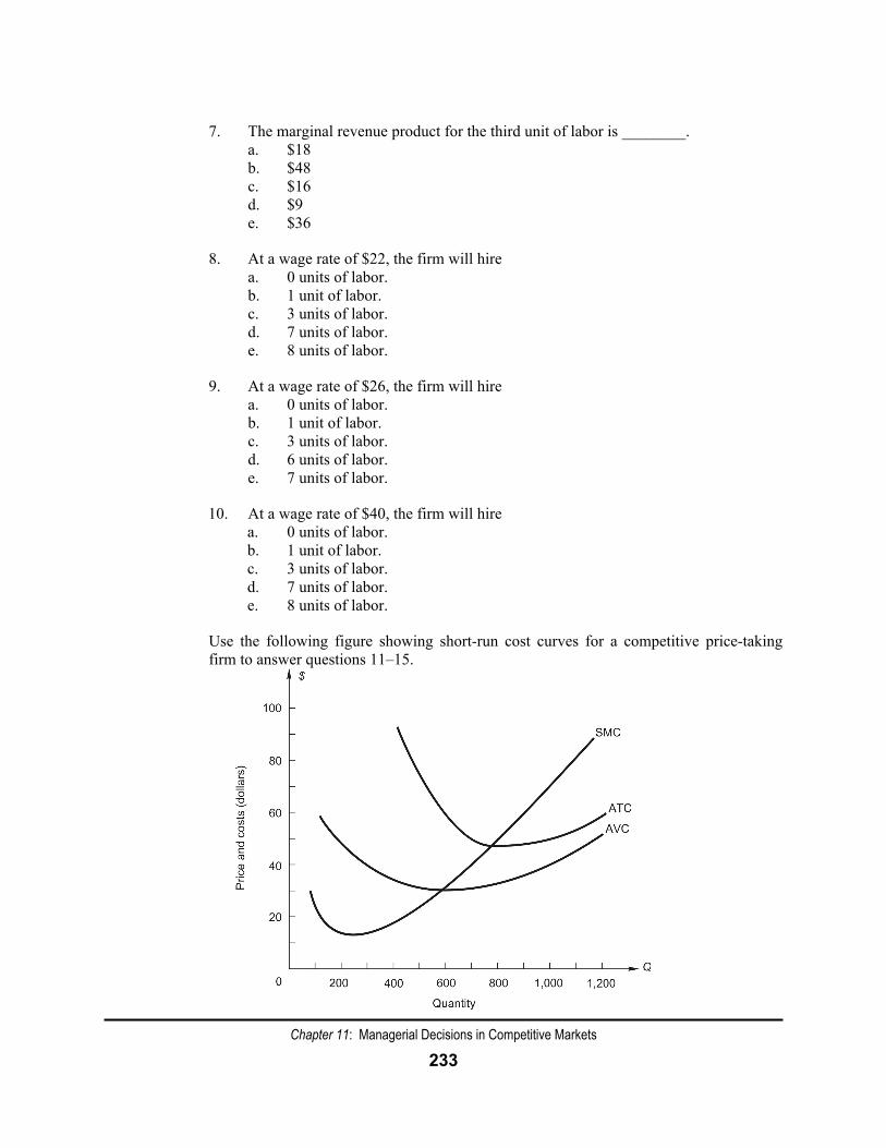
Use the following figure showing short-run cost curves for a competitive price-taking firm to answer questions 11–15.


234

11. If price is $70 how much does the firm produce? a. 750 units b. 1,000 units c. 900 units d. 600 units

12. If price is $70 how much profit (loss) does the firm make? a. zero b. $16,500 c. $20,000 d. $23,000 e. $15,500

13. Let price be $40. How much does the firm produce? a. zero units b. 500 units c. 600 units d. 700 units e. 800 units

14. If price is $40, how much profit (loss) does the firm make? a. it loses its fixed cost b. $5,000 c. –$7,000 d. –$4,000 e. $3,500

15. Below what price will the firm shut down and produce nothing? a. $48 b. $18 c. $20 d. $30 e. $50


235

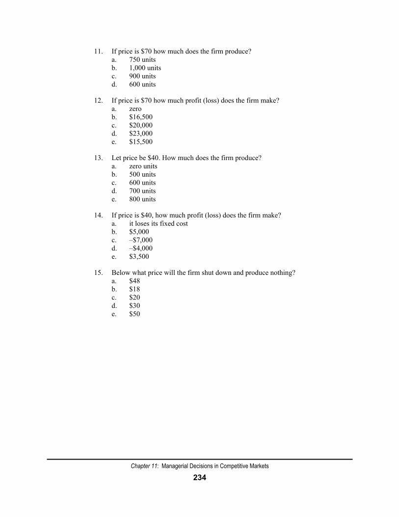
Use the following figure showing long-run cost curves for the typical firm in a perfectly competitive industry, to answer questions 16–19.

16. If price is $40, the firm will produce ________ units. a. 2,000 b. 3,000 c. 4,000 d. 4,500 e. 5,000

17. If price is $40, how much profit (loss) does the firm make? a. $75,000 b. $60,000 c. $50,000 d. $10,000 e. zero

18. If price is $40 and the firm produces the optimal level of output in this period, what is likely to occur next period? a. Each firm will increase output. b. Price will fall. c. Firms will exit the market. d. b and c. e. all of the above.


236

19. If this industry is in long-run competitive equilibrium the firm will produce ________units of output and price will be ________. a. 1,000; $15 b. 2,000; $20 c. 3,000; $20 d. 4,000; $22 e. 4,500; $30

For questions 20–28, use the following data for a competitive industry and a price-taking firm that operates in this market. Using time-series data, the market demand and supply functions are estimated to be

Demand: ˆ 550 10 0.01Q P M= − + Supply: ˆ 400 10 12.5 IQ P P= + −

where output is Q, the price of the product is P, income is M, and the price of a key input is PI. The income forecasted for 2012 is $30,000 and the price of inputs is $52. Jartech, Inc. is a firm operating in this market. Jartech’s average variable cost function is estimated to be

2ˆ 60.0 0.08 0.0001AVC Q Q= − + where ˆAVC is measured in dollars per unit. Jartech expects to face total fixed costs of $2,500 in 2012.

20. What is the price forecast for 2012? a. $15 b. $20 c. $35 d. $40 e. $55

21. At what output level will Jartech’s average variable cost reach its minimum value? a. 200 units b. 300 units c. 400 units d. 500 units e. 600 units

22. What is the minimum average variable cost? a. $0 b. $55 c. $45 d. $44 e. $20

23. The profit-maximizing (or loss-minimizing) output for Jartech is a. 0 units. b. 300 units. c. 400 units. d. 500 units. e. 600 units.


237

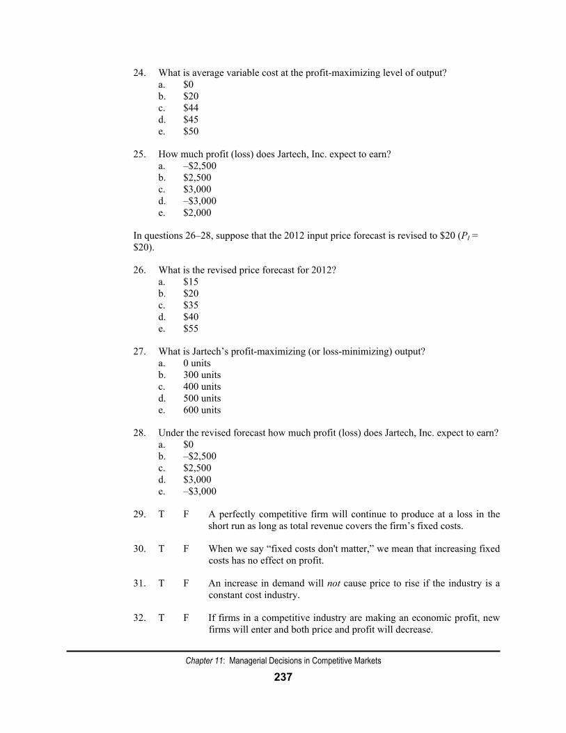
24. What is average variable cost at the profit-maximizing level of output? a. $0 b. $20 c. $44 d. $45 e. $50

25. How much profit (loss) does Jartech, Inc. expect to earn? a. –$2,500 b. $2,500 c. $3,000 d. –$3,000 e. $2,000

In questions 26–28, suppose that the 2012 input price forecast is revised to $20 (PI = $20).

26. What is the revised price forecast for 2012? a. $15 b. $20 c. $35 d. $40 e. $55

27. What is Jartech’s profit-maximizing (or loss-minimizing) output? a. 0 units b. 300 units c. 400 units d. 500 units e. 600 units

28. Under the revised forecast how much profit (loss) does Jartech, Inc. expect to earn? a. $0 b. –$2,500 c. $2,500 d. $3,000 e. –$3,000

29. T F A perfectly competitive firm will continue to produce at a loss in the short run as long as total revenue covers the firm’s fixed costs.

30. T F When we say “fixed costs don't matter,” we mean that increasing fixed costs has no effect on profit.

31. T F An increase in demand will not cause price to rise if the industry is a constant cost industry.

32. T F If firms in a competitive industry are making an economic profit, new firms will enter and both price and profit will decrease.


238

33. T F If the owner’s superior managerial ability is keeping the firm’s costs below those of other firms, the firm will earn economic profit in long-run competitive equilibrium.

34. T F If price is greater than marginal cost, the firm should produce less. Answers

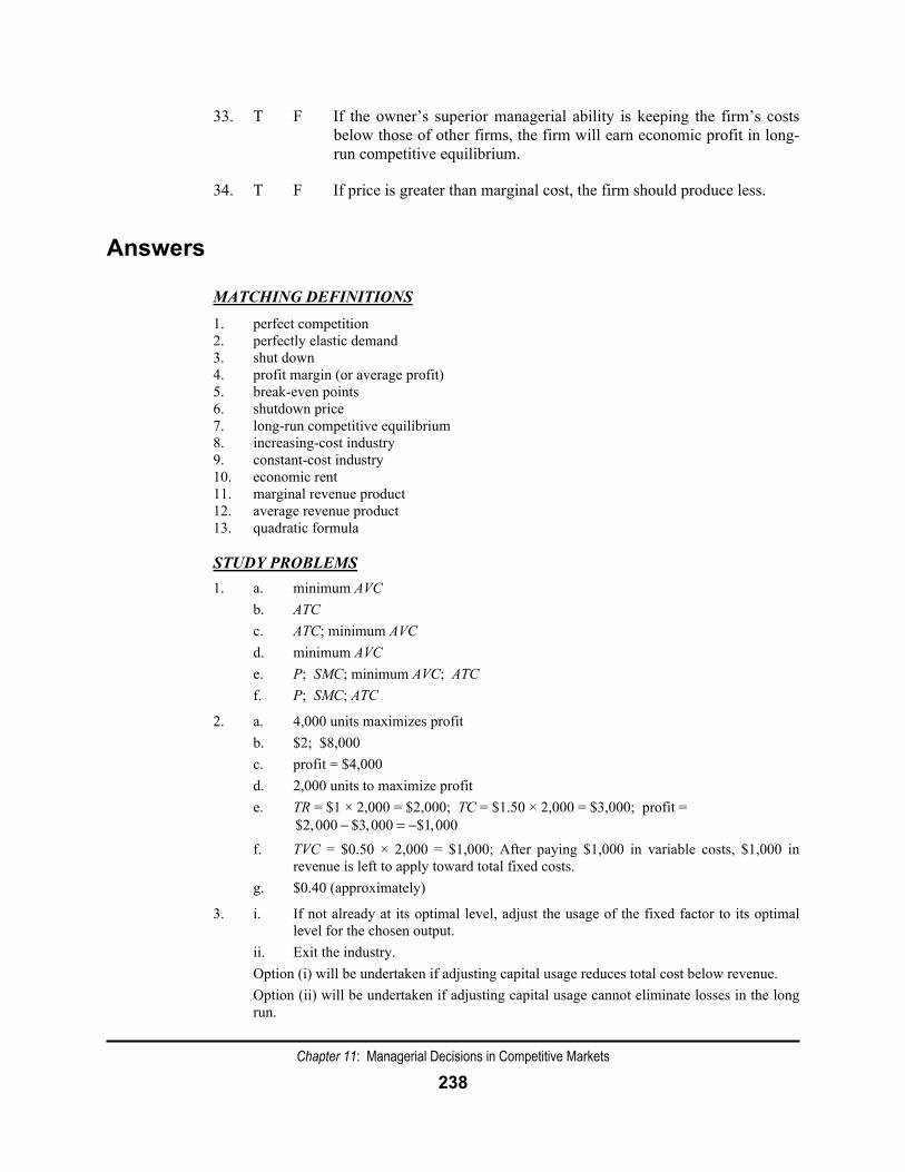
MATCHING DEFINITIONS 1. perfect competition 2. perfectly elastic demand 3. shut down 4. profit margin (or average profit) 5. break-even points 6. shutdown price 7. long-run competitive equilibrium 8. increasing-cost industry 9. constant-cost industry 10. economic rent 11. marginal revenue product 12. average revenue product 13. quadratic formula

STUDY PROBLEMS 1. a. minimum AVC

b. ATC c. ATC; minimum AVC d. minimum AVC e. P; SMC; minimum AVC; ATC f. P; SMC; ATC

2. a. 4,000 units maximizes profit b. $2; $8,000 c. profit = $4,000 d. 2,000 units to maximize profit e. TR = $1 × 2,000 = $2,000; TC = $1.50 × 2,000 = $3,000; profit =

$2,000 $3,000 $1,000− = − f. TVC = $0.50 × 2,000 = $1,000; After paying $1,000 in variable costs, $1,000 in

revenue is left to apply toward total fixed costs. g. $0.40 (approximately)

3. i. If not already at its optimal level, adjust the usage of the fixed factor to its optimal level for the chosen output.

ii. Exit the industry. Option (i) will be undertaken if adjusting capital usage reduces total cost below revenue. Option (ii) will be undertaken if adjusting capital usage cannot eliminate losses in the long run.


239

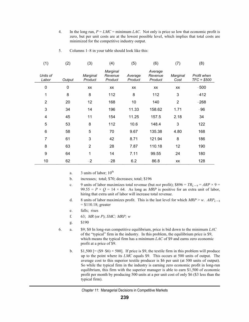
4. In the long run, P = LMC = minimum LAC. Not only is price so low that economic profit is zero, but per unit costs are at the lowest possible level, which implies that total costs are minimized for the competitive industry output.

5. Columns 1–8 in your table should look like this:

(1) (2) (3) (4) (5) (6) (7) (8)

Units of Labor

Output

Marginal Product


Average Product


Marginal

Cost Profit when TFC = $500

0 0 xx xx xx xx xx –500

1 8 8 112 8 112 3 –412

2 20 12 168 10 140 2 –268

3 34 14 196 11.33 158.62 1.71 –96

4 45 11 154 11.25 157.5 2.18 34

5 53 8 112 10.6 148.4 3 122

6 58 5 70 9.67 135.38 4.80 168

7 61 3 42 8.71 121.94 8 186

8 63 2 28 7.87 110.18 12 190

9 64 1 14 7.11 99.55 24 180

10 62 –2 –28 6.2 86.8 xx 128

a. 3 units of labor; 10th b. increases; total; $70; decreases; total; $196 c. 9 units of labor maximizes total revenue (but not profit); $896 = TRL = 9 = ARP × 9 =

99.55 = P × Q = 14 × 64. As long as MRP is positive for an extra unit of labor, hiring that extra unit of labor will increase total revenue.

d. 8 units of labor maximizes profit. This is the last level for which MRP > w. ARPL = 8 = $110.18; greater

e. falls; rises f. 63; MR (or P); SMC; MRP; w g. $190

6. a. $9; $0 In long-run competitive equilibrium, price is bid down to the minimum LAC of the “typical” firm in the industry. In this problem, the equilibrium price is $9, which means the typical firm has a minimum LAC of $9 and earns zero economic profit at a price of $9.

b. $1,500 [= ($9–$6) × 500]. If price is $9, the textile firm in this problem will produce up to the point where its LMC equals $9. This occurs at 500 units of output. The average cost to this superior textile producer is $6 per unit (at 500 units of output). So while the typical firm in the industry is earning zero economic profit in long-run equilibrium, this firm with the superior manager is able to earn $1,500 of economic profit per month by producing 500 units at a per unit cost of only $6 ($3 less than the typical firm).


240

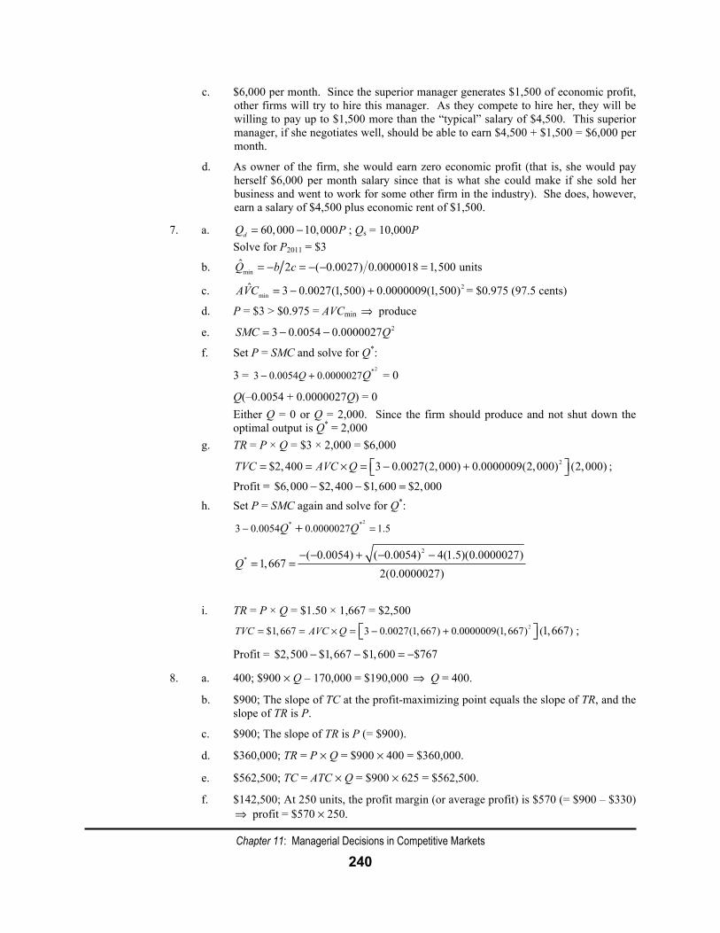
c. $6,000 per month. Since the superior manager generates $1,500 of economic profit, other firms will try to hire this manager. As they compete to hire her, they will be willing to pay up to $1,500 more than the “typical” salary of $4,500. This superior manager, if she negotiates well, should be able to earn $4,500 + $1,500 = $6,000 per month.

d. As owner of the firm, she would earn zero economic profit (that is, she would pay herself $6,000 per month salary since that is what she could make if she sold her business and went to work for some other firm in the industry). She does, however, earn a salary of $4,500 plus economic rent of $1,500.

7. a. 60,000 10,000dQ P= − ; Qs = 10,000P Solve for P2011 = $3

b. minˆ 2 ( 0.0027) 0.0000018 1,500 unitsQ b c= − = − − =

c. 2min

ˆ 3 0.0027(1,500) 0.0000009(1,500)AVC = − + = $0.975 (97.5 cents)

d. P = $3 > $0.975 = AVCmin ⇒ produce

e. 23 0.0054 0.0000027SMC Q= − −

f. Set P = SMC and solve for Q*:

3 = 2*3 0.0054 0.0000027Q Q− + = 0

Q(–0.0054 + 0.0000027Q) = 0 Either Q = 0 or Q = 2,000. Since the firm should produce and not shut down the

optimal output is Q* = 2,000 g. TR = P × Q = $3 × 2,000 = $6,000

2$2,400 3 0.0027(2,000) 0.0000009(2,000) (2,000)TVC AVC Q= = × = − +⎡ ⎤⎣ ⎦ ;

Profit = $6,000 $2,400 $1,600 $2,000− − = h. Set P = SMC again and solve for Q*:

2* *3 0.0054 0.0000027 1.5Q Q− =+

2* ( 0.0054) ( 0.0054) 4(1.5)(0.0000027)1,667

2(0.0000027)Q

− − + − −= =

i. TR = P × Q = $1.50 × 1,667 = $2,500

2$1, 667 3 0.0027(1, 667) 0.0000009(1, 667) ( )1,667TVC AVC Q= = × = − +⎡ ⎤⎣ ⎦ ;

Profit = $2,500 $1,667 $1,600 $767− − = −

8. a. 400; $900 × Q – 170,000 = $190,000 ⇒ Q = 400.

b. $900; The slope of TC at the profit-maximizing point equals the slope of TR, and the slope of TR is P.

c. $900; The slope of TR is P (= $900).

d. $360,000; TR = P × Q = $900 × 400 = $360,000.

e. $562,500; TC = ATC × Q = $900 × 625 = $562,500.

f. $142,500; At 250 units, the profit margin (or average profit) is $570 (= $900 – $330) ⇒ profit = $570 × 250.


241

g. –$50,000; At Q = 0, profit = –TFC. At 250 units, ATC = $330 and AVC = $130, so TFC = ($330 – $130) × 250.

h. $570; The 250th unit adds $900 to total revenue and adds $330 to total cost, and so increases profit by $570 (= $900 – $330). Thus, the slope of the profit function must be $570 at 250 units.

i. $425; ATC = TC/Q ⇒ ATC = $170,000/400 ⇒ ATC = $425.

i. 60; Since P = ATC at j, it is a break-even point. In the top panel, the break-even point occurs at 60 units.

k. $820; Since TFC = $50,000 (see part g), it follows that ($900 – AVC) × 625 = $50,000. Solving for AVC ⇒ AVC = $820.

9. a. At 250 units, AFC is $200 (= $330 – $130), and at 650 units, AFC is $80 (=$900 – $820). At 250 units, TFC is $50,000 (= $200 × 250), and at 650 units, TFC is $50,000 (=$80 × 625). As Q increases, AFC declines continuously while TFC is constant.

b. Break-even points occur at 60 and 625 units of output. At 60 units, the line tangent to TC is flatter than TR. Thus, in the bottom panel of the figure in Study Problem 8, SMC (which is the value of the slope of the line tangent to TC at 60 units) must be less than MR (which is the slope of TR and equals P). At 650 units, the line tangent to TC is steeper than TR. At 650 units, SMC (which is the value of the slope of the line tangent to TC at 650 units) must be greater than MR.

c. At 400 units, profit reaches its maximum value because the slope of TR equals the slope of TC (i.e., MR = SMC). Since the 400th unit adds $900 to TR and adds $900 to TC, the change in profit is zero and the tangent line has zero slope at the peak of the profit hill.

d. Profit margin (or average profit) is maximized where ATC is minimized, which occurs at 250 units in this problem. By increasing output from 250 to 400 units, the firm can increase its profit by $47,500 (= $190,000 – $142,500).

e. Your response: “Yes, increasing production to 500 units will indeed increase revenues by $90,000. Unfortunately, total costs will increase by more than $90,000 because marginal cost exceeds $900 (i.e., MR) for all of these 100 extra units. Thus, increasing output from 400 to 500 units will decrease profit.”

MULTIPLE CHOICE / TRUE-FALSE

1. a Perfectly competitive firms do not view each other as fierce rivals because each firm

is so small relative to the total market that no one firm’s increase in sales prevents any other firm from selling as much as it wishes to at the going market price.

2. a When demand is horizontal, P = MR, and demand is perfectly elastic. 3. d TR < TVC ⇒ P < AVC ⇒ shut down and MRP > ARP ⇒ shut down 4. c Choice c is really P > AVC in disguise since TR/Q = P. 5. d Since ATC = 30 and AFC = 5, AVC must be 25. You are told that SMC = 25, so the

firm must be producing at the minimum point on AVC. Since P = 24 < AVCmin, the firm should shut down.

6. e In long-run competitive equilibrium, P = LMC = LAC = SMC = ATC, and profit = 0. 7. e MRPL=3 = MPL=3 × P = 18 × $2 = $36 8. d MRPL=7 = $24 > $22 > MRPL=8 = $20 9. d MRPL=6 = $28 > $26 > MRPL=7 = $24


242

10. a At the level of labor usage for which MRP = $40 (i.e., L = 2), MRPL=2 = 40 > 30 = ARPL = 2 ⇒ shut down

11. b P = SMC = $70 at Q = 1,000 12. c $20,000 ( ) (70 50)1,000P ATC Q= − = −

13. d SMC = P = $40 at Q = 700 14. c $7,000 ( ) (40 50)700P ATC Q− = − = −

15. d Minimum AVC = $30 16. e P = SMC = $40 at Q = 5,000 17. a $75,000 ( ) (40 25)5,000P LAC Q= − = −

18. b Price falls because new firms enter and increase supply. 19. c Minimum LAC equals $20; 3,000 20. e 850 10 250 10P P− = − + ⇒ P = $55

21. c minˆˆ ˆ2 400 (0.08) 0.0002Q b c= − = = −

22. d 2min

ˆ $44 60 0.08(400) 0.0001(400)AVC = = − +

23. d 2 *60 0.16 0.0003 $55 500SMC Q Q Q= − + = ⇒ =

24. d 2500

ˆ $45 60 0.08(500) 0.0001(500)QAVC = = = − +

25. b Profit ($55 500) ($45 500) $2,500 $2,500= × − × − =

26. c 850 10 150 10 $35P P P− = + ⇒ =

27. a minˆ $45 shut downP AVC< = ⇒

28. b Profit = –TFC = –$2,500 29. F It is variable costs that must be covered in order to produce. 30. F Increasing fixed cost does decrease profit. The level of fixed cost does not affect the

production decision. If P < AVC, the firm shuts down no matter how high or low fixed costs are. If P ≥ AVC, the firm produces the level of output where MR = SMC, no matter how high or low fixed costs are.

31. T A constant-cost industry has a horizontal long-run industry supply curve. In the long-run, an increase in demand will not lead to an increase in price. [Note: In the short-run, the short-run industry supply curve is upward sloping, even for a constant cost industry, and an increase in demand will cause price to rise in the short run.]

32. T Entry takes place when economic profits are positive and entry increases supply. 33. F The owner will earn a normal profit plus rent. 34. F Produce more if P > SMC


243

Homework Exercises

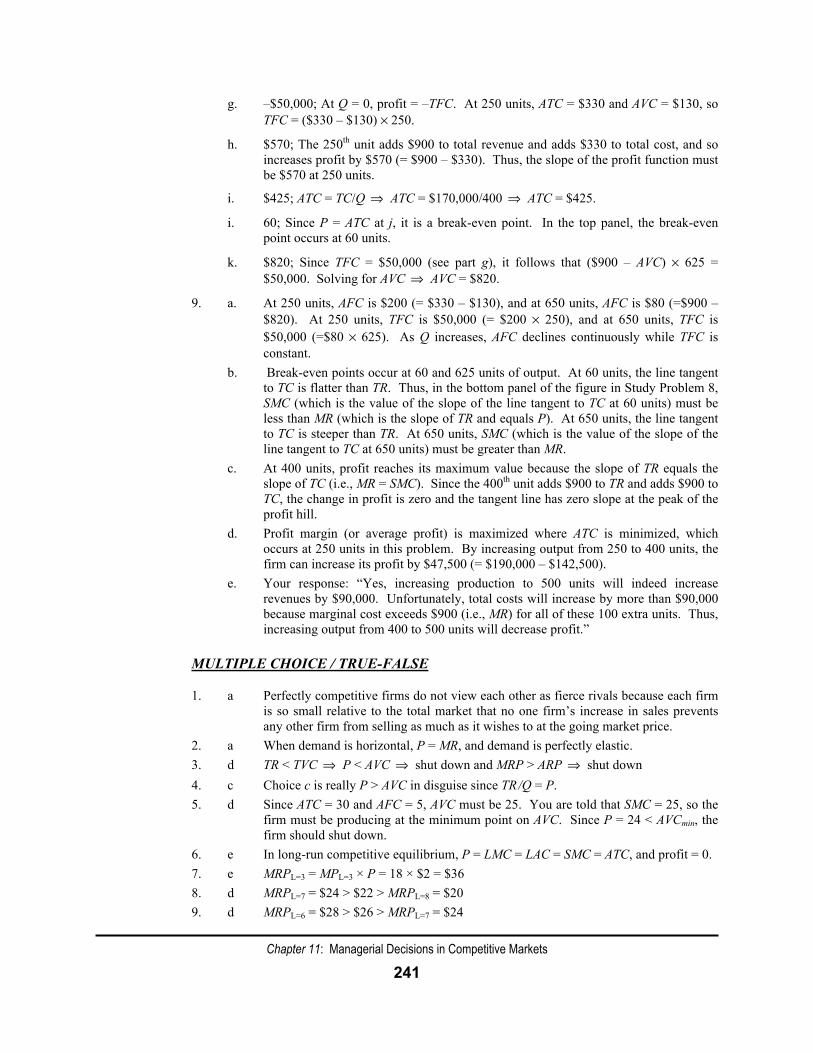
1. Consider the cost curves for a price-taking firm in the following figure:

a. When price is $12 per unit of output, the firm maximizes profit by producing

__________ units.

b. Since average total cost = $___________ for this output, total cost is

$____________.

c. The firm makes an economic profit (loss) of $____________________.

d. Price falls to $8. The firm now maximizes profit by producing ______ units.

e. At this output level, total revenue = $__________ and total cost =

$____________. Therefore the firm earns a profit (loss) of $____________.

f. Price falls to $6. The firm now maximizes profit by producing

_____________ units.

g. At this output level, average total cost is $_________ and total cost is

$_____________. Total revenue = $____________ and the firm makes a

loss of $________________.

h. Even though the firm makes a loss, it does not shut down because total

variable cost is $____________, which leaves $_________ of total revenue

to apply toward fixed costs.

i. If price falls below $_____________, the firm shuts down. Explain why.


244

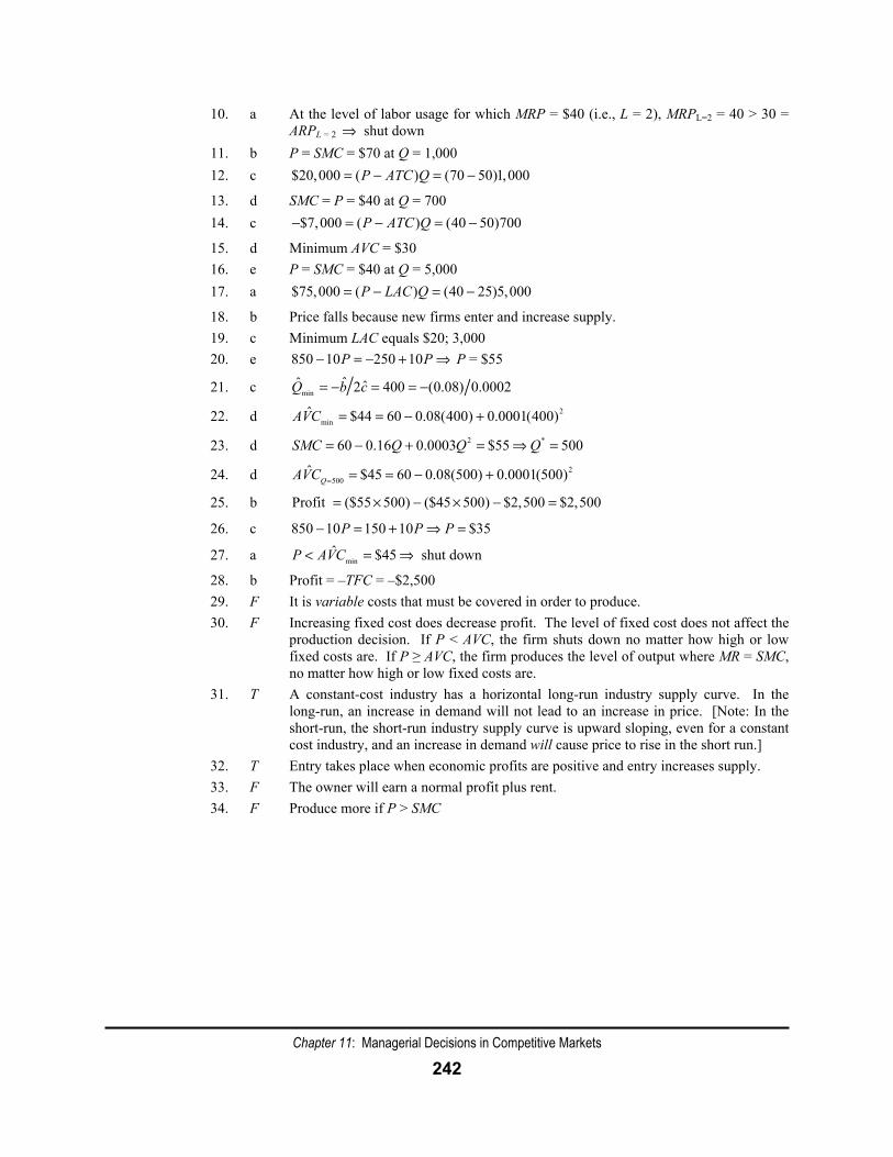
2. Ajax Corporation is a price-taking firm in a competitive industry that employs only one variable input, labor, to produce a product that sells for $2 per unit. The wage rate is $8 per unit of labor and total fixed costs are $1,000. Fill in the blanks in each column of this table as instructed by the questions below:

(1) (2) (3) (4) (5) (6) (7) (8)

Units of Labor

Output

Marginal Product


Average Product


Marginal

Cost

Profit

0 0 xx xx xx xx xx ______

1 400 ______ ______ ______ ______ ______ ______

2 950 ______ ______ ______ ______ ______ ______

3 1,250 ______ ______ ______ ______ ______ ______

4 1,350 ______ ______ ______ ______ ______ ______

5 1,370 ______ ______ ______ ______ ______ ______

6 1,373 ______ ______ ______ ______ ______ ______

7 1,369 ______ ______ ______ ______ ______ ______

8 1,364 ______ ______ ______ ______ ______ ______

a. Fill in the blanks in columns 3 and 5. Marginal product begins to diminish beyond ________ units of labor. Marginal product is negative beyond _________ units of labor.

b. Compute marginal and average revenue products and fill in the blanks in columns 4 and 6. The sixth unit of labor __________________ (increases, decreases) total revenue by $__________. Decreasing labor usage from four to three units _______________ (increases, decreases) total revenue by $_________.

c. The manager can maximize total revenue by hiring ________ units of labor. The maximum possible value of total revenue is $____________.

d. The manager hires ________ units of labor and produces ___________ units of output in order to maximize profit. At this level of labor usage, ARP = _____________ which is ______________ (greater, less) than MRP.

e. Compute marginal cost and fill in the blanks in column 7. At first, marginal cost ___________ (rises, falls) as marginal product rises, then marginal cost _____________ (rises, falls) as marginal product falls.

f. The profit-maximizing level of output is ______ units because this is the last level of output for which _____________ exceeds _____________, or equivalently, _____________ exceeds _____________ .


245

g. Compute profit and fill in the blanks in column 8. The optimal level of labor

employment and the optimal level of output both result in an identical

maximum profit level of $_____________.

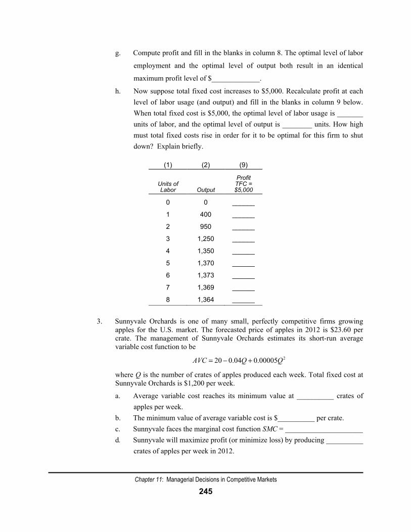
h. Now suppose total fixed cost increases to $5,000. Recalculate profit at each level of labor usage (and output) and fill in the blanks in column 9 below. When total fixed cost is $5,000, the optimal level of labor usage is _______ units of labor, and the optimal level of output is ________ units. How high must total fixed costs rise in order for it to be optimal for this firm to shut down? Explain briefly.

(1) (2) (9)

Units of Labor

Output

Profit TFC = $5,000

0 0 ______

1 400 ______

2 950 ______

3 1,250 ______

4 1,350 ______

5 1,370 ______

6 1,373 ______

7 1,369 ______

8 1,364 ______

3. Sunnyvale Orchards is one of many small, perfectly competitive firms growing

apples for the U.S. market. The forecasted price of apples in 2012 is $23.60 per crate. The management of Sunnyvale Orchards estimates its short-run average variable cost function to be

220 0.04 0.00005AVC Q Q= − +

where Q is the number of crates of apples produced each week. Total fixed cost at Sunnyvale Orchards is $1,200 per week.

a. Average variable cost reaches its minimum value at __________ crates of apples per week.

b. The minimum value of average variable cost is $__________ per crate. c. Sunnyvale faces the marginal cost function SMC = _____________________ d. Sunnyvale will maximize profit (or minimize loss) by producing __________

crates of apples per week in 2012.


246

e. Sunnyvale’s profit will be $__________ per week. [Note: If a loss occurs, then express profit as a negative value.]

f. If the price of apples falls to $10 per crate, Sunnyvale should produce _____ crates per week, and its profit will be $_________per week. [Note: If a loss occurs, then express profit as a negative value.]

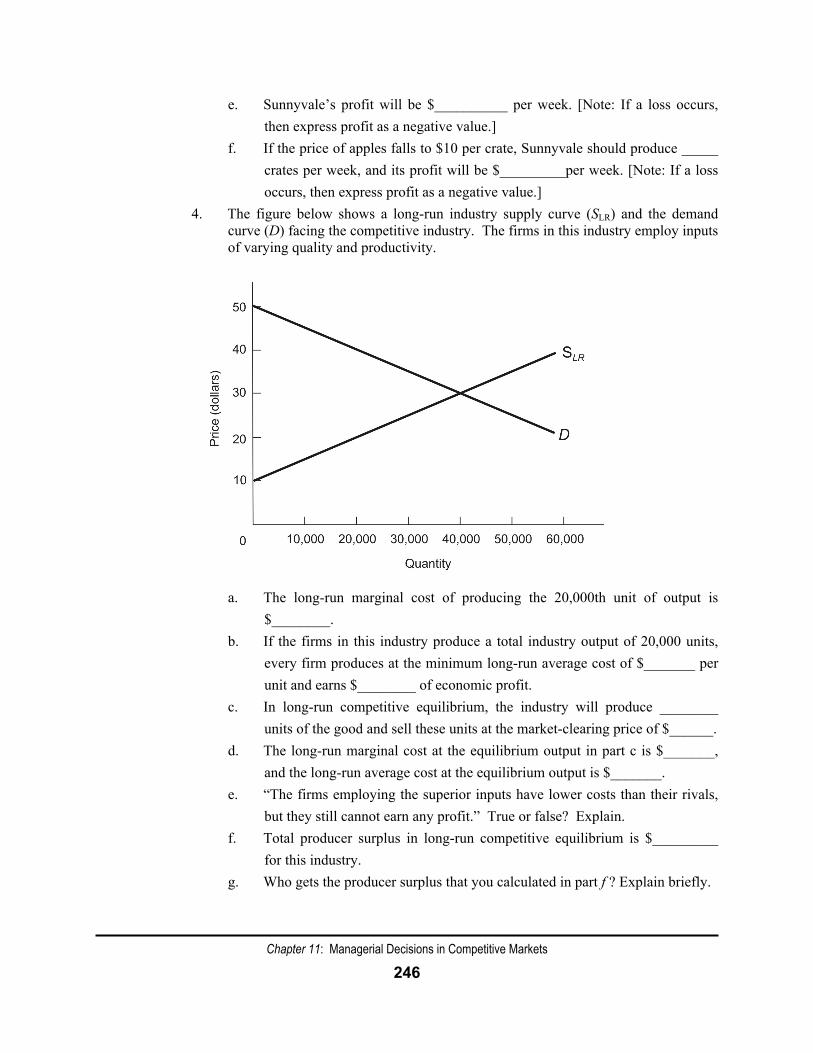
4. The figure below shows a long-run industry supply curve (SLR) and the demand curve (D) facing the competitive industry. The firms in this industry employ inputs of varying quality and productivity.

a. The long-run marginal cost of producing the 20,000th unit of output is $________.

b. If the firms in this industry produce a total industry output of 20,000 units, every firm produces at the minimum long-run average cost of $_______ per unit and earns $________ of economic profit.

c. In long-run competitive equilibrium, the industry will produce ________ units of the good and sell these units at the market-clearing price of $______.

d. The long-run marginal cost at the equilibrium output in part c is $_______, and the long-run average cost at the equilibrium output is $_______.

e. “The firms employing the superior inputs have lower costs than their rivals, but they still cannot earn any profit.” True or false? Explain.

f. Total producer surplus in long-run competitive equilibrium is $_________ for this industry.

g. Who gets the producer surplus that you calculated in part f ? Explain briefly.

Documents

10e 11 Chap Student Workbook - University of Daytonacademic.udayton.edu/MBA790/Student Workbook/10e_11_Chap_St… · this Workbook, you should be able to: Discuss three characteristics