Embed Size (px)
Citation preview
13.1Database System Concepts - 6th Edition
Chapter 13: Query OptimizationChapter 13: Query Optimization
Introduction
Transformation of Relational Expressions
Catalog Information for Cost Estimation
Cost-based optimization
Heuristic optimization
Statistical Information for Cost Estimation
#Optimizing Nested Subqueries
#Materialized views
13.2Database System Concepts - 6th Edition
IntroductionIntroduction
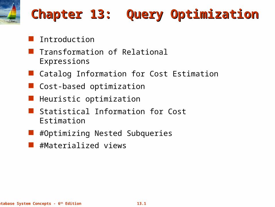
Alternative ways of evaluating a given query
Equivalent expressions
Different algorithms for each operation
13.3Database System Concepts - 6th Edition
Introduction (Cont.)Introduction (Cont.)
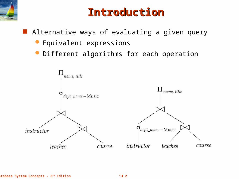
An evaluation plan defines exactly what algorithm is used for each operation, and how the execution of the operations is coordinated.
Find out how to view query execution plans on your favorite database
13.4Database System Concepts - 6th Edition
Introduction (Cont.)Introduction (Cont.)
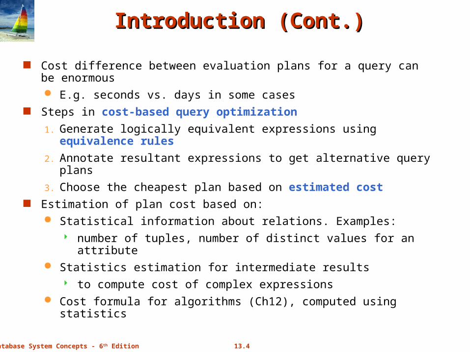
Cost difference between evaluation plans for a query can be enormous E.g. seconds vs. days in some cases
Steps in cost-based query optimization
1. Generate logically equivalent expressions using equivalence rules
2. Annotate resultant expressions to get alternative query plans
3. Choose the cheapest plan based on estimated cost Estimation of plan cost based on:
Statistical information about relations. Examples: number of tuples, number of distinct values for an attribute
Statistics estimation for intermediate results to compute cost of complex expressions
Cost formula for algorithms (Ch12), computed using statistics
13.5Database System Concepts - 6th Edition
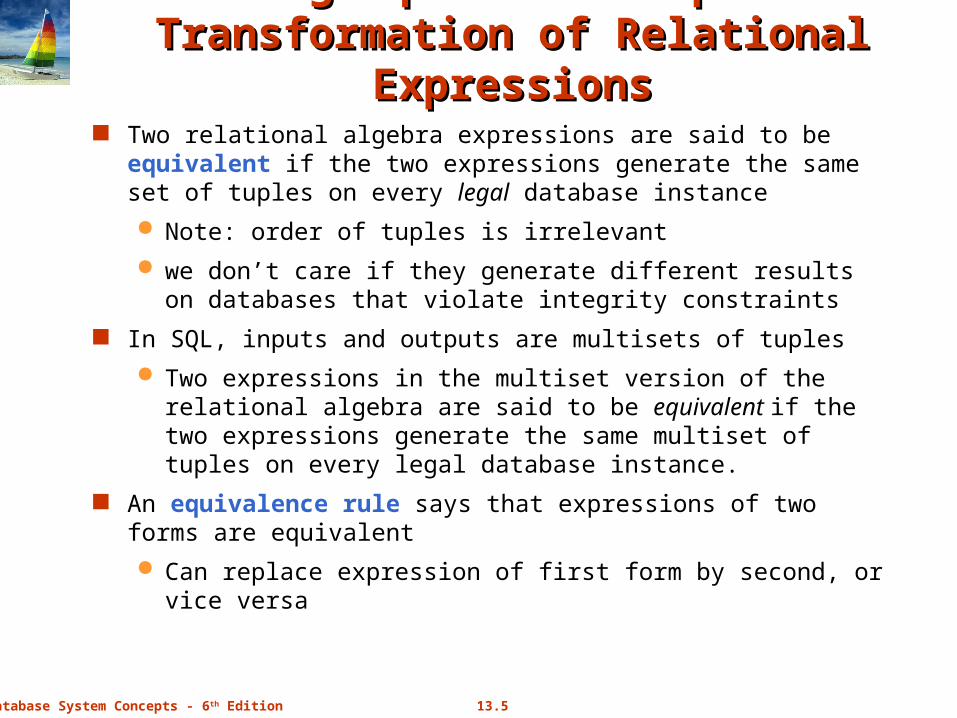
Generating Equivalent Expressions-Generating Equivalent Expressions-Transformation of Relational ExpressionsTransformation of Relational Expressions Two relational algebra expressions are said to be equivalent if
the two expressions generate the same set of tuples on every legal database instance
Note: order of tuples is irrelevant
we don’t care if they generate different results on databases that violate integrity constraints
In SQL, inputs and outputs are multisets of tuples
Two expressions in the multiset version of the relational algebra are said to be equivalent if the two expressions generate the same multiset of tuples on every legal database instance.
An equivalence rule says that expressions of two forms are equivalent
Can replace expression of first form by second, or vice versa
13.6Database System Concepts - 6th Edition
Equivalence RulesEquivalence Rules
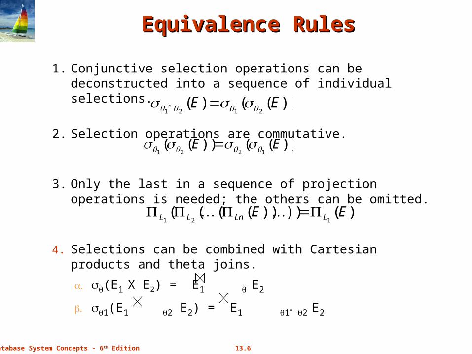
1. Conjunctive selection operations can be deconstructed into a sequence of individual selections.
2. Selection operations are commutative.
3. Only the last in a sequence of projection operations is needed; the others can be omitted.
4. Selections can be combined with Cartesian products and theta joins.
a. (E1 X E2) = E1 E2
b. 1(E1 2 E2) = E1 1 2 E2
))(())((1221EE
))(()(2121EE
)())))((((121EE LLnLL
13.7Database System Concepts - 6th Edition
Equivalence Rules (Cont.)Equivalence Rules (Cont.)
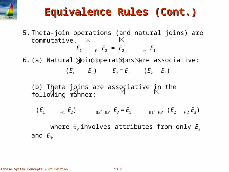
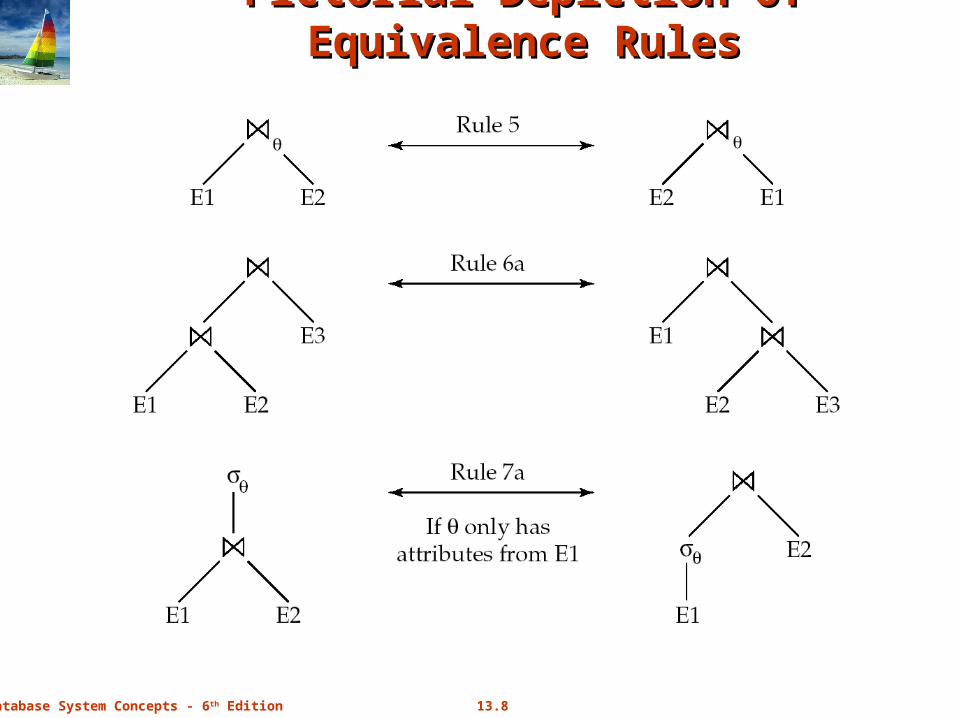
5. Theta-join operations (and natural joins) are commutative.E1 E2 = E2 E1
6. (a) Natural join operations are associative:
(E1 E2) E3 = E1 (E2 E3)
(b) Theta joins are associative in the following manner:
(E1 1 E2) 2 3 E3 = E1 1 3 (E2 2 E3)
where 2 involves attributes from only E2 and E3.
13.8Database System Concepts - 6th Edition
Pictorial Depiction of Equivalence RulesPictorial Depiction of Equivalence Rules
13.9Database System Concepts - 6th Edition
Equivalence Rules (Cont.)Equivalence Rules (Cont.)
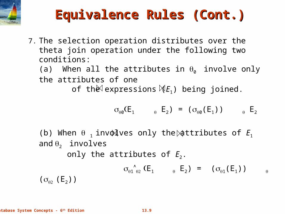
7. The selection operation distributes over the theta join operation under the following two conditions:(a) When all the attributes in 0 involve only the attributes of one of the expressions (E1) being joined.
0E1 E2) = (0(E1)) E2
(b) When 1 involves only the attributes of E1 and 2 involves only the attributes of E2.
1 E1 E2) = (1(E1)) ( (E2))
13.10Database System Concepts - 6th Edition
Equivalence Rules (Cont.)Equivalence Rules (Cont.)
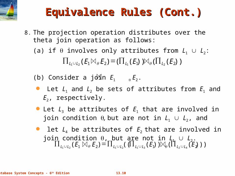
8. The projection operation distributes over the theta join operation as follows:
(a) if involves only attributes from L1 L2:
(b) Consider a join E1 E2.
Let L1 and L2 be sets of attributes from E1 and E2, respectively.
Let L3 be attributes of E1 that are involved in join condition , but are not in L1 L2, and
let L4 be attributes of E2 that are involved in join condition , but are not in L1 L2.
))(())(()( 2121 2121EEEE LLLL
)))(())((()( 2121 42312121EEEE LLLLLLLL
13.11Database System Concepts - 6th Edition
Equivalence Rules (Cont.)Equivalence Rules (Cont.)
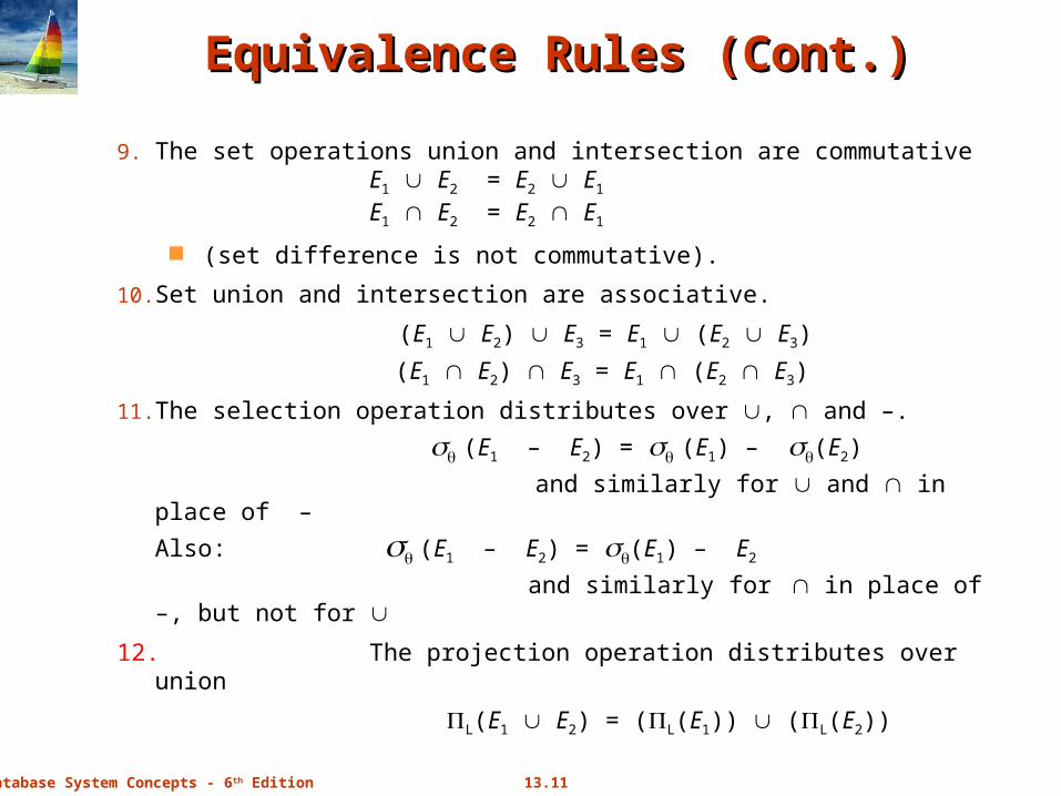
9. The set operations union and intersection are commutative E1 E2 = E2 E1 E1 E2 = E2 E1
(set difference is not commutative).
10. Set union and intersection are associative.
(E1 E2) E3 = E1 (E2 E3)
(E1 E2) E3 = E1 (E2 E3)
11. The selection operation distributes over , and –.
(E1 – E2) = (E1) – (E2)
and similarly for and in place of –
Also: (E1 – E2) = (E1) – E2
and similarly for in place of –, but not for
12. The projection operation distributes over union
L(E1 E2) = (L(E1)) (L(E2))
13.12Database System Concepts - 6th Edition
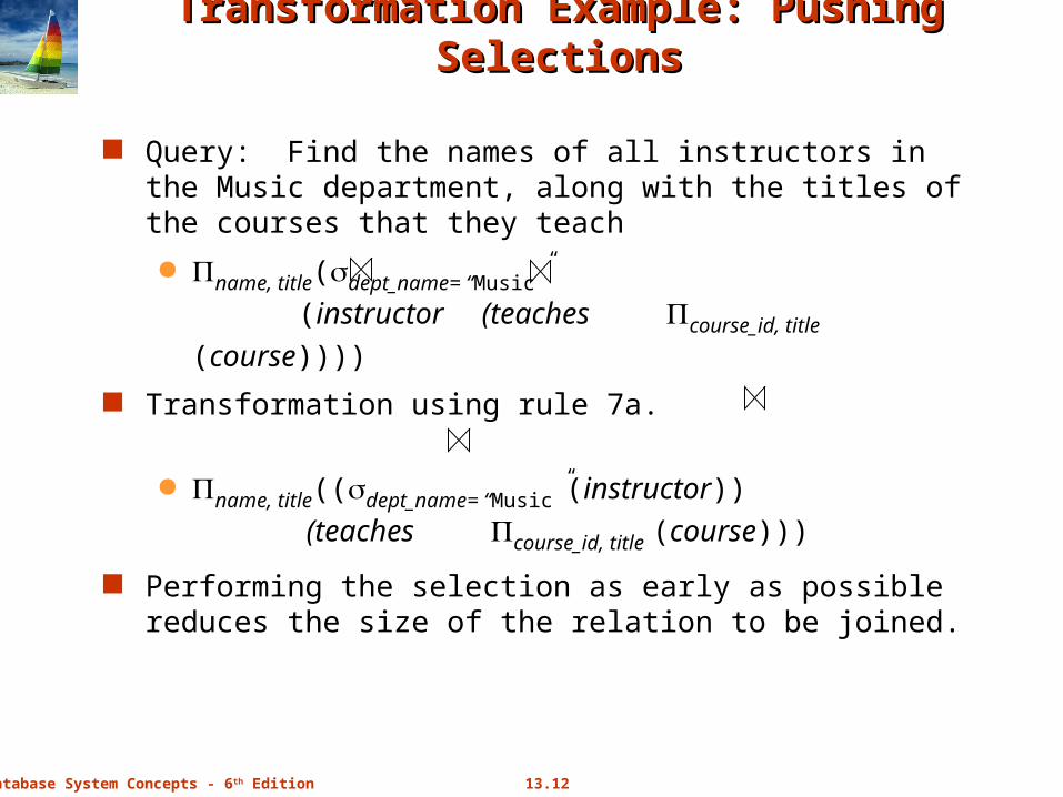
Transformation Example: Pushing SelectionsTransformation Example: Pushing Selections
Query: Find the names of all instructors in the Music department, along with the titles of the courses that they teach
name, title(dept_name= “Music”
(instructor (teaches course_id, title (course))))
Transformation using rule 7a.
name, title((dept_name= “Music”(instructor))
(teaches course_id, title (course)))
Performing the selection as early as possible reduces the size of the relation to be joined.
13.13Database System Concepts - 6th Edition
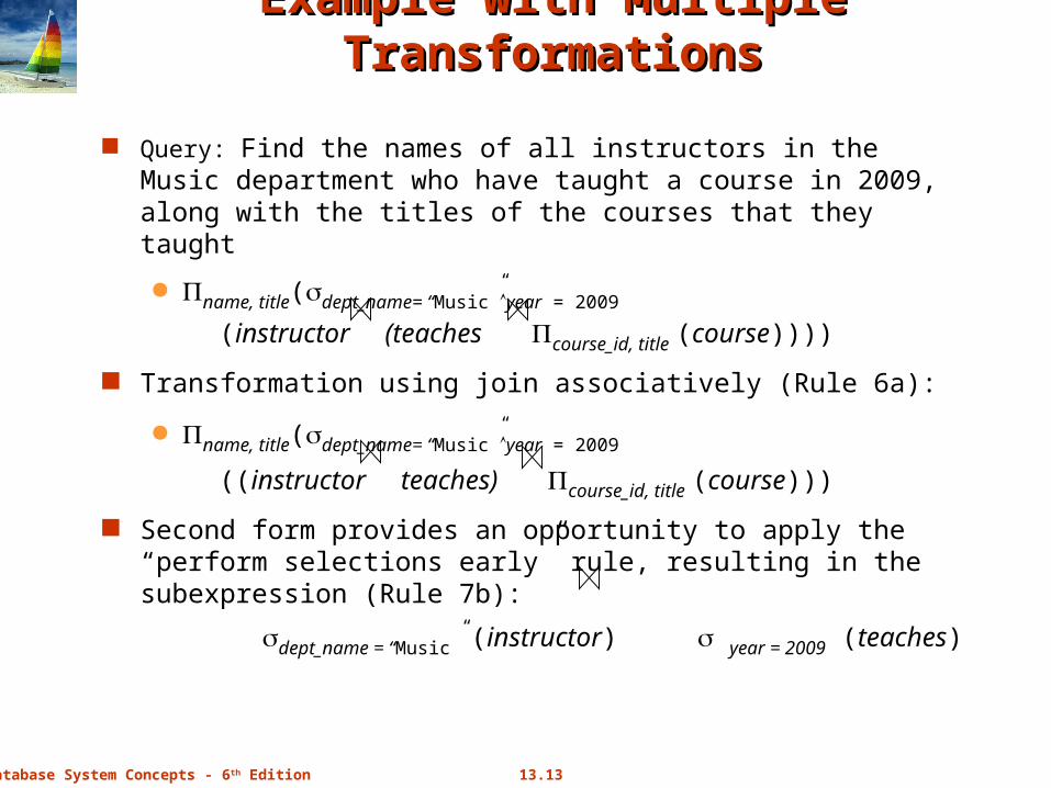
Example with Multiple TransformationsExample with Multiple Transformations
Query: Find the names of all instructors in the Music department who have taught a course in 2009, along with the titles of the courses that they taught
name, title(dept_name= “Music”year = 2009
(instructor (teaches course_id, title (course))))
Transformation using join associatively (Rule 6a):
name, title(dept_name= “Music”year = 2009
((instructor teaches) course_id, title (course)))
Second form provides an opportunity to apply the “perform selections early” rule, resulting in the subexpression (Rule 7b):
dept_name = “Music” (instructor) year = 2009 (teaches)
13.14Database System Concepts - 6th Edition
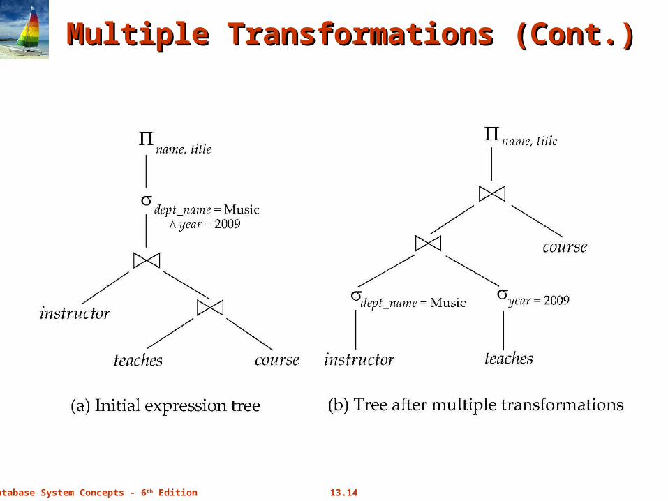
Multiple Transformations (Cont.)Multiple Transformations (Cont.)
13.15Database System Concepts - 6th Edition
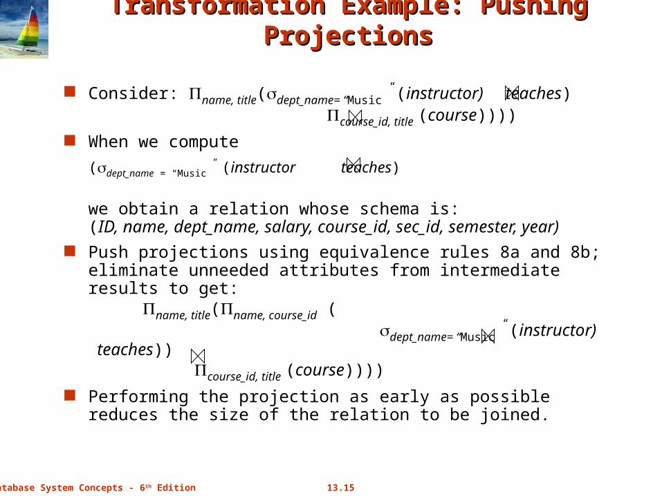
Transformation Example: Pushing ProjectionsTransformation Example: Pushing Projections
Consider: name, title(dept_name= “Music” (instructor) teaches) course_id, title (course))))
When we compute
(dept_name = “Music” (instructor teaches)
we obtain a relation whose schema is:(ID, name, dept_name, salary, course_id, sec_id, semester, year)
Push projections using equivalence rules 8a and 8b; eliminate unneeded attributes from intermediate results to get: name, title(name, course_id ( dept_name= “Music” (instructor) teaches)) course_id, title (course))))
Performing the projection as early as possible reduces the size of the relation to be joined.
13.16Database System Concepts - 6th Edition
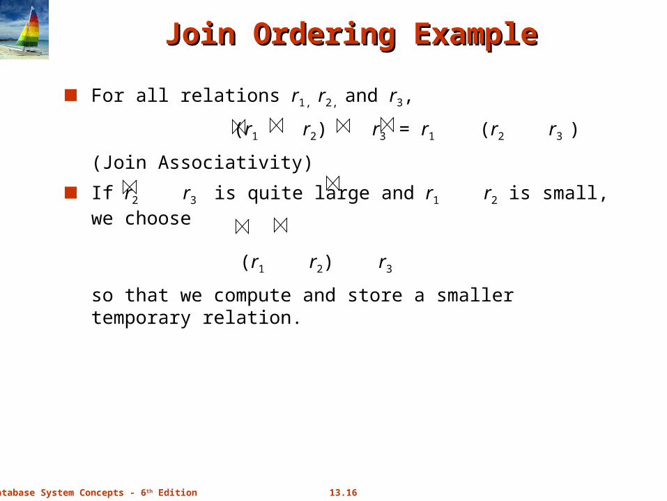
Join Ordering ExampleJoin Ordering Example
For all relations r1, r2, and r3,
(r1 r2) r3 = r1 (r2 r3 )
(Join Associativity)
If r2 r3 is quite large and r1 r2 is small, we choose
(r1 r2) r3
so that we compute and store a smaller temporary relation.
13.17Database System Concepts - 6th Edition
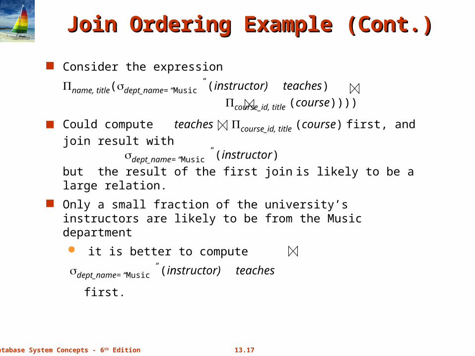
Join Ordering Example (Cont.)Join Ordering Example (Cont.)
Consider the expression
name, title(dept_name= “Music” (instructor) teaches)
course_id, title (course))))
Could compute teaches course_id, title (course) first, and
join result with dept_name= “Music” (instructor)
but the result of the first join is likely to be a large relation.
Only a small fraction of the university’s instructors are likely to be from the Music department
it is better to compute
dept_name= “Music” (instructor) teaches
first.
13.18Database System Concepts - 6th Edition
Enumeration of Equivalent ExpressionsEnumeration of Equivalent Expressions
Query optimizers use equivalence rules to systematically generate expressions equivalent to the given expression
Can generate all equivalent expressions as follows:
Repeat
apply all applicable equivalence rules on every subexpression of every equivalent expression found so far
add newly generated expressions to the set of equivalent expressions
Until no new equivalent expressions are generated above
The above approach is very expensive in space and time
Two approaches
Optimized plan generation based on transformation rules
Special case approach for certain queries
13.19Database System Concepts - 6th Edition
Implementing Transformation Based Implementing Transformation Based OptimizationOptimization
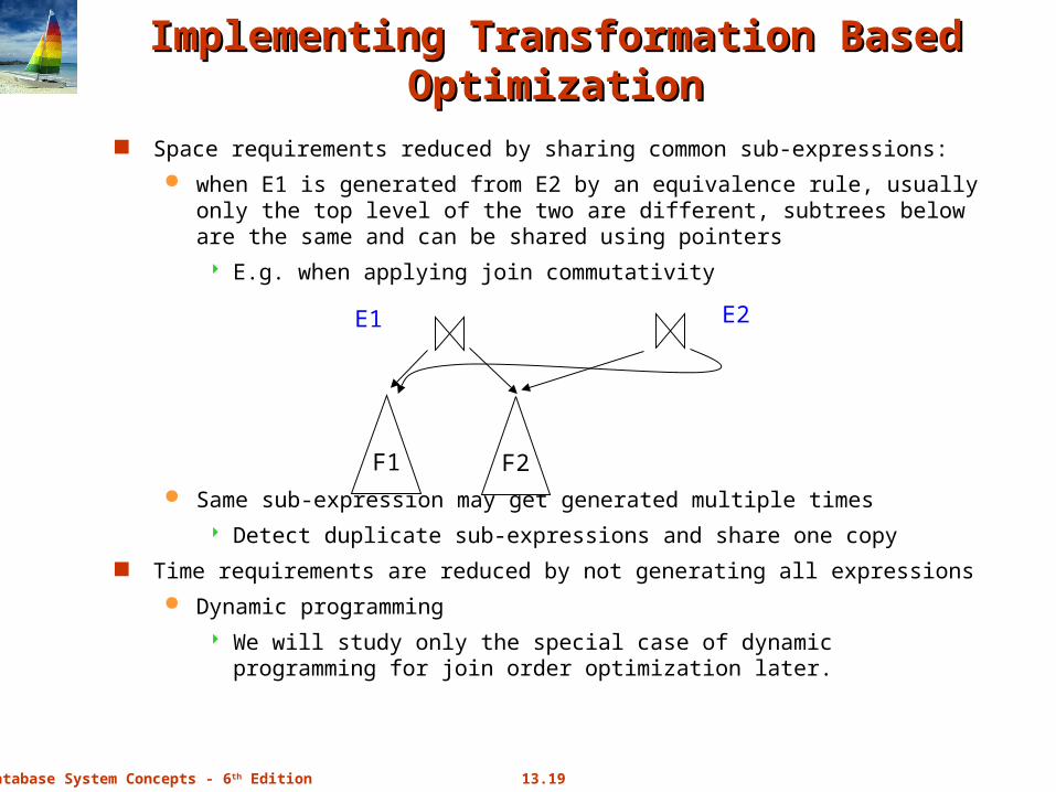
Space requirements reduced by sharing common sub-expressions:
when E1 is generated from E2 by an equivalence rule, usually only the top level of the two are different, subtrees below are the same and can be shared using pointers
E.g. when applying join commutativity
Same sub-expression may get generated multiple times
Detect duplicate sub-expressions and share one copy
Time requirements are reduced by not generating all expressions
Dynamic programming
We will study only the special case of dynamic programming for join order optimization later.
F1 F2
E1 E2
13.20Database System Concepts - 6th Edition
Choice of Evaluation PlansChoice of Evaluation Plans
Must consider the interaction of evaluation techniques when choosing evaluation plans
choosing the cheapest algorithm for each operation independently may not yield best overall algorithm. E.g.
merge-join may be costlier than hash-join, but may provide a sorted output which reduces the cost for an outer level aggregation.
nested-loop join may provide opportunity for pipelining
Practical query optimizers incorporate elements of the following two broad approaches:
1. Search all the plans and choose the best plan in a cost-based fashion.
2. Uses heuristics to choose a plan.
13.21Database System Concepts - 6th Edition
Cost-Based OptimizationCost-Based Optimization
Consider finding the best join-order for r1 r2 . . . rn.
There are (2(n – 1))!/(n – 1)! different join orders for above expression. With n = 7, the number is 665280, with n = 10, the number is greater than 176 billion!
No need to generate all the join orders. Using dynamic programming, the least-cost join order for any subset of {r1, r2, . . . rn} is computed only once and stored for future use.
13.22Database System Concepts - 6th Edition
Dynamic Programming in OptimizationDynamic Programming in Optimization
To find best join tree for a set of n relations:
To find best plan for a set S of n relations, consider all possible plans of the form: S1 (S – S1) where S1 is any non-empty subset of S.
Recursively compute costs for joining subsets of S to find the cost of each plan. Choose the cheapest of all the alternatives (around 2n ).
Base case for recursion: single relation access plan
Apply all selections on Ri using best choice of indices on Ri
When plan for any subset is computed, store it and reuse it when it is required again, instead of recomputing it
Dynamic programming
13.23Database System Concepts - 6th Edition
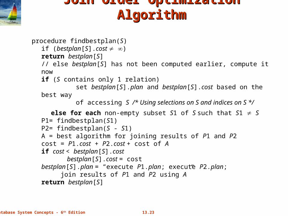
Join Order Optimization AlgorithmJoin Order Optimization Algorithm
procedure findbestplan(S)if (bestplan[S].cost )
return bestplan[S]// else bestplan[S] has not been computed earlier, compute it nowif (S contains only 1 relation) set bestplan[S].plan and bestplan[S].cost based on the best way of accessing S /* Using selections on S and indices on S */
else for each non-empty subset S1 of S such that S1 SP1= findbestplan(S1)P2= findbestplan(S - S1)A = best algorithm for joining results of P1 and P2cost = P1.cost + P2.cost + cost of Aif cost < bestplan[S].cost
bestplan[S].cost = costbestplan[S].plan = “execute P1.plan; execute P2.plan;
join results of P1 and P2 using A”return bestplan[S]
13.24Database System Concepts - 6th Edition
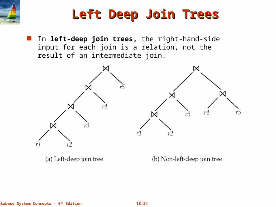
Left Deep Join TreesLeft Deep Join Trees
In left-deep join trees, the right-hand-side input for each join is a relation, not the result of an intermediate join.
13.25Database System Concepts - 6th Edition
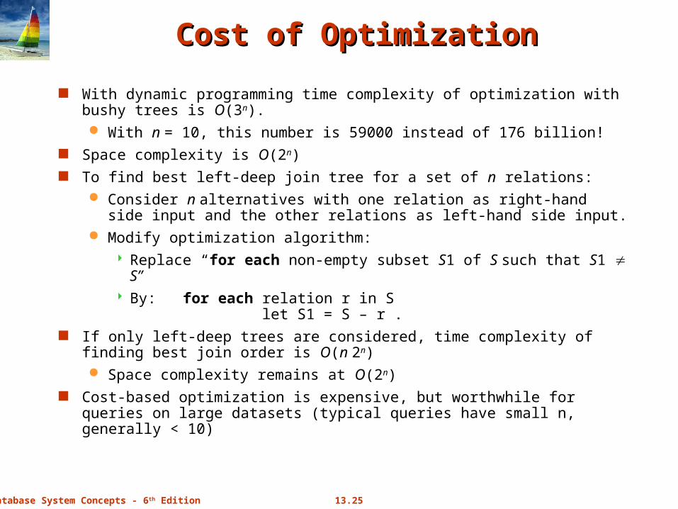
Cost of OptimizationCost of Optimization
With dynamic programming time complexity of optimization with bushy trees is O(3n). With n = 10, this number is 59000 instead of 176 billion!
Space complexity is O(2n) To find best left-deep join tree for a set of n relations:
Consider n alternatives with one relation as right-hand side input and the other relations as left-hand side input.
Modify optimization algorithm: Replace “for each non-empty subset S1 of S such that S1 S” By: for each relation r in S
let S1 = S – r . If only left-deep trees are considered, time complexity of finding best join
order is O(n 2n) Space complexity remains at O(2n)
Cost-based optimization is expensive, but worthwhile for queries on large datasets (typical queries have small n, generally < 10)
13.26Database System Concepts - 6th Edition
Interesting Sort OrdersInteresting Sort Orders
Consider the expression (r1 r2) r3 (with A as common attribute)
An interesting sort order is a particular sort order of tuples that could be useful for a later operation
Using merge-join to compute r1 r2 may be costlier than hash join but generates result sorted on A
Which in turn may make merge-join with r3 cheaper, which may reduce cost of join with r3 and minimizing overall cost
Sort order may also be useful for order by and for grouping
Not sufficient to find the best join order for each subset of the set of n given relations
must find the best join order for each subset, for each interesting sort order
Simple extension of earlier dynamic programming algorithms
Usually, number of interesting orders is quite small and doesn’t affect time/space complexity significantly
13.27Database System Concepts - 6th Edition
Cost Based Optimization with Equivalence Rules
Physical equivalence rules allow logical query plan to be converted to physical query plan specifying what algorithms are used for each operation.
Efficient optimizer based on equivalent rules depends on
A space efficient representation of expressions which avoids making multiple copies of subexpressions
Efficient techniques for detecting duplicate derivations of expressions
A form of dynamic programming based on memoization, which stores the best plan for a subexpression the first time it is optimized, and reuses in on repeated optimization calls on same subexpression
Cost-based pruning techniques that avoid generating all plans
Pioneered by the Volcano project and implemented in the SQL Server optimizer
13.28Database System Concepts - 6th Edition
Heuristic OptimizationHeuristic Optimization
Cost-based optimization is expensive, even with dynamic programming.
Systems may use heuristics to reduce the number of choices that must be made in a cost-based fashion.
Heuristic optimization transforms the query-tree by using a set of rules that typically (but not in all cases) improve execution performance:
Perform selection early (reduces the number of tuples)
Perform projection early (reduces the number of attributes)
Perform most restrictive selection and join operations (i.e. with smallest result size) before other similar operations.
Some systems use only heuristics, others combine heuristics with partial cost-based optimization.
13.29Database System Concepts - 6th Edition
Structure of Query OptimizersStructure of Query Optimizers
Many optimizers considers only left-deep join orders.
Plus heuristics to push selections and projections down the query tree
Reduces optimization complexity and generates plans amenable to pipelined evaluation.
Heuristic optimization used in some versions of Oracle:
Repeatedly pick “best” relation to join next
Starting from each of n starting points. Pick best among these
Intricacies of SQL complicate query optimization
E.g. nested subqueries
13.30Database System Concepts - 6th Edition
Structure of Query Optimizers (Cont.)Structure of Query Optimizers (Cont.)
Some query optimizers integrate heuristic selection and the generation of alternative access plans.
Frequently used approach
heuristic rewriting of nested block structure and aggregation
followed by cost-based join-order optimization for each block
Some optimizers (e.g. SQL Server) apply transformations to entire query and do not depend on block structure
Optimization cost budget to stop optimization early (if cost of plan is less than cost of optimization)
Plan caching to reuse previously computed plan if query is resubmitted
Even with different constants in query
Even with the use of heuristics, cost-based query optimization imposes a substantial overhead.
But is worth it for expensive queries
Optimizers often use simple heuristics for very cheap queries, and perform exhaustive enumeration for more expensive queries
13.31Database System Concepts - 6th Edition
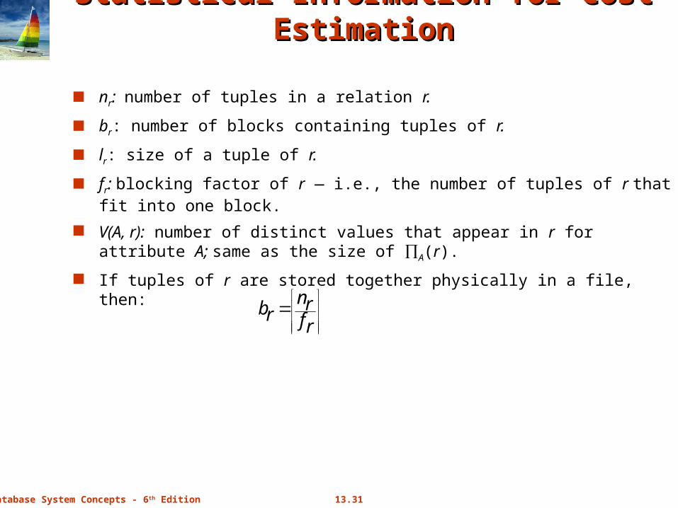
Statistical Information for Cost EstimationStatistical Information for Cost Estimation
nr: number of tuples in a relation r.
br: number of blocks containing tuples of r.
lr: size of a tuple of r.
fr: blocking factor of r — i.e., the number of tuples of r that fit into one block.
V(A, r): number of distinct values that appear in r for attribute A; same as the size of A(r).
If tuples of r are stored together physically in a file, then:
rfrn
rb
13.32Database System Concepts - 6th Edition
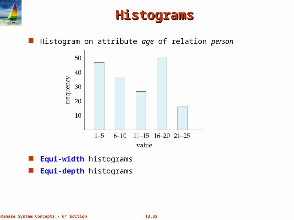
HistogramsHistograms
Histogram on attribute age of relation person
Equi-width histograms
Equi-depth histograms
13.33Database System Concepts - 6th Edition
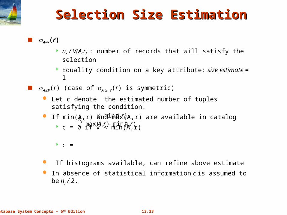
Selection Size EstimationSelection Size Estimation
A=v(r)
nr / V(A,r) : number of records that will satisfy the selection
Equality condition on a key attribute: size estimate = 1
AV(r) (case of A V(r) is symmetric)
Let c denote the estimated number of tuples satisfying the condition.
If min(A,r) and max(A,r) are available in catalog
c = 0 if v < min(A,r)
c =
If histograms available, can refine above estimate
In absence of statistical information c is assumed to be nr / 2.
),min(),max(
),min(.
rArA
rAvnr
13.34Database System Concepts - 6th Edition
Size Estimation of Complex SelectionsSize Estimation of Complex Selections
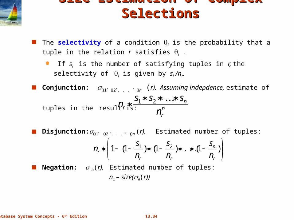
The selectivity of a condition i is the probability that a tuple in the relation r
satisfies i .
If si is the number of satisfying tuples in r, the selectivity of i is given by si /nr.
Conjunction: 1 2. . . n (r). Assuming indepdence, estimate of
tuples in the result is:
Disjunction:1 2 . . . n (r). Estimated number of tuples:
Negation: (r). Estimated number of tuples:
nr – size((r))
nr
nr n
sssn
. . . 21
)1(...)1()1(1 21
r
n
rrr n
s
n
s
n
sn
13.35Database System Concepts - 6th Edition
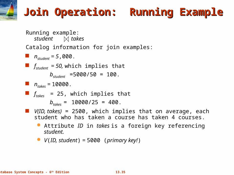
Join Operation: Running ExampleJoin Operation: Running Example
Running example: student takes
Catalog information for join examples:
nstudent = 5,000.
fstudent = 50, which implies that
bstudent =5000/50 = 100.
ntakes = 10000.
ftakes = 25, which implies that
btakes = 10000/25 = 400.
V(ID, takes) = 2500, which implies that on average, each student who has taken a course has taken 4 courses. Attribute ID in takes is a foreign key referencing student. V(ID, student) = 5000 (primary key!)
13.36Database System Concepts - 6th Edition
Estimation of the Size of JoinsEstimation of the Size of Joins
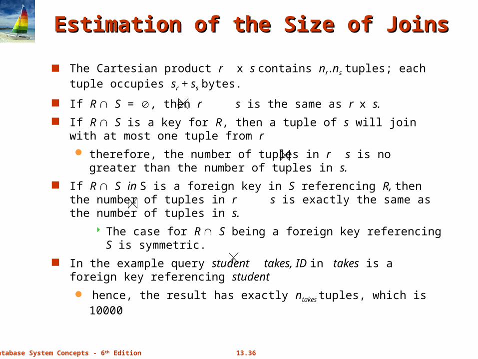
The Cartesian product r x s contains nr .ns tuples; each tuple occupies sr + ss bytes.
If R S = , then r s is the same as r x s.
If R S is a key for R, then a tuple of s will join with at most one tuple from r
therefore, the number of tuples in r s is no greater than the number of tuples in s.
If R S in S is a foreign key in S referencing R, then the number of tuples in r s is exactly the same as the number of tuples in s.
The case for R S being a foreign key referencing S is symmetric.
In the example query student takes, ID in takes is a foreign key referencing student
hence, the result has exactly ntakes tuples, which is 10000
13.37Database System Concepts - 6th Edition
Estimation of the Size of Joins (Cont.)Estimation of the Size of Joins (Cont.)
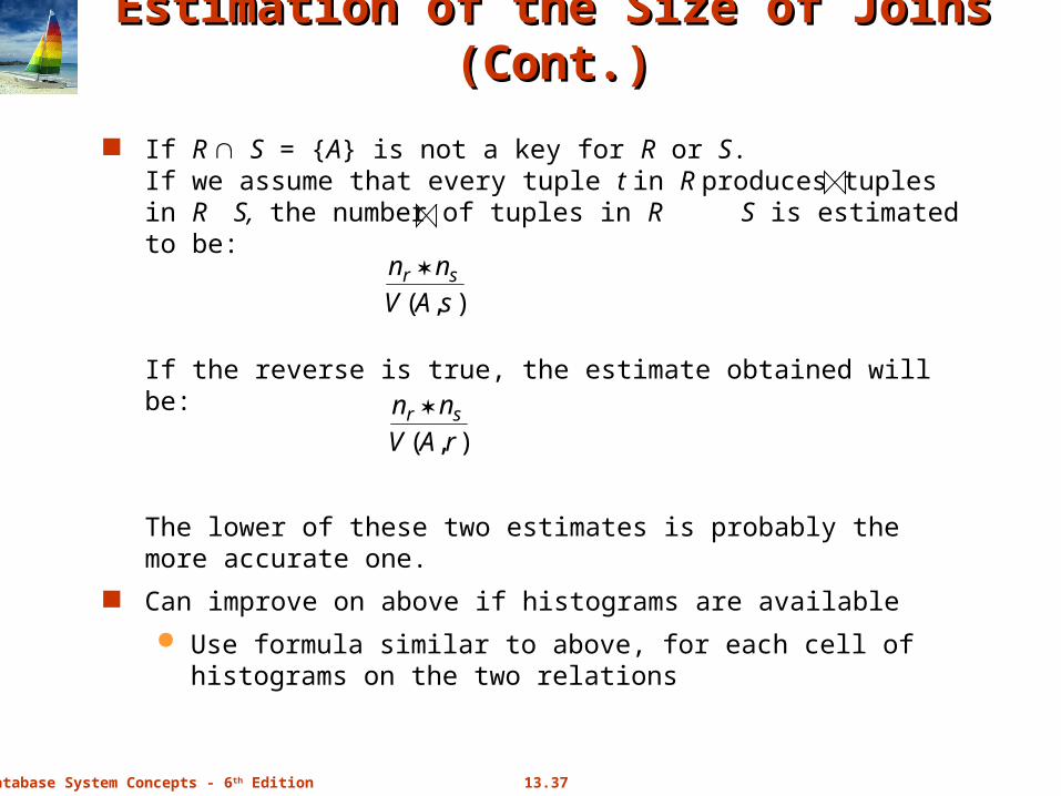
If R S = {A} is not a key for R or S.If we assume that every tuple t in R produces tuples in R S, the number of tuples in R S is estimated to be:
If the reverse is true, the estimate obtained will be:
The lower of these two estimates is probably the more accurate one.
Can improve on above if histograms are available
Use formula similar to above, for each cell of histograms on the two relations
),( sAVnn sr
),( rAVnn sr
13.38Database System Concepts - 6th Edition
Estimation of the Size of Joins (Cont.)Estimation of the Size of Joins (Cont.)
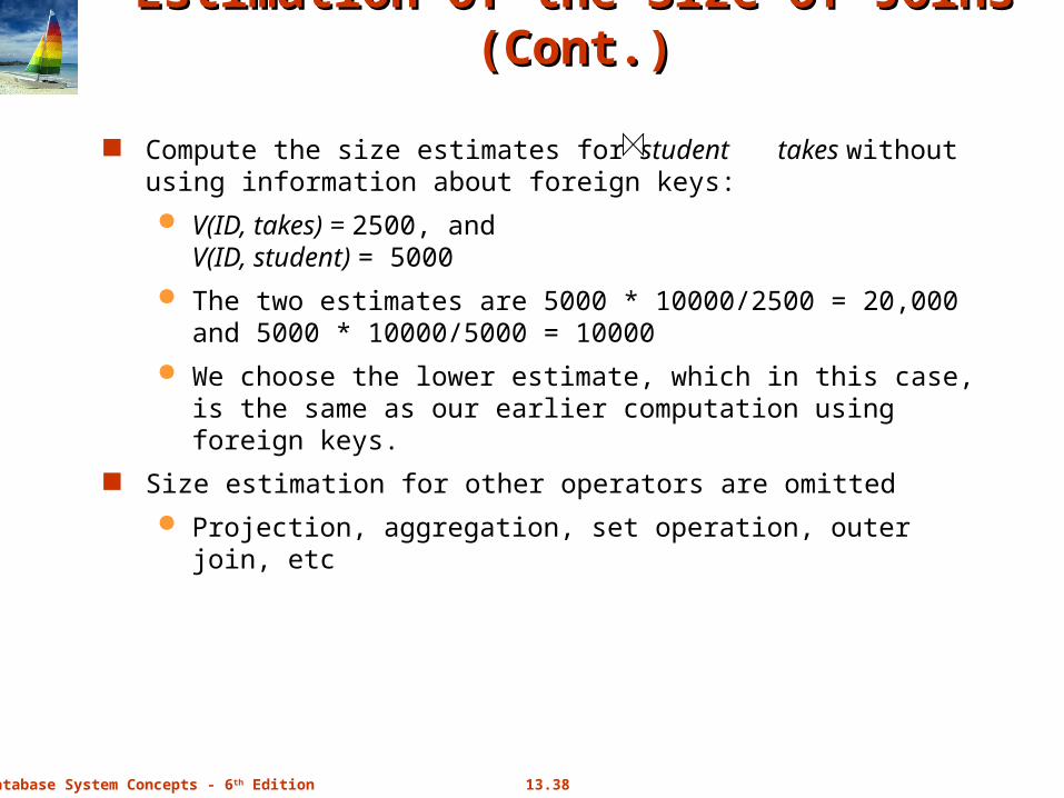
Compute the size estimates for student takes without using information about foreign keys:
V(ID, takes) = 2500, andV(ID, student) = 5000
The two estimates are 5000 * 10000/2500 = 20,000 and 5000 * 10000/5000 = 10000
We choose the lower estimate, which in this case, is the same as our earlier computation using foreign keys.
Size estimation for other operators are omitted
Projection, aggregation, set operation, outer join, etc
13.39Database System Concepts - 6th Edition
Optimizing Nested Subqueries**Optimizing Nested Subqueries**
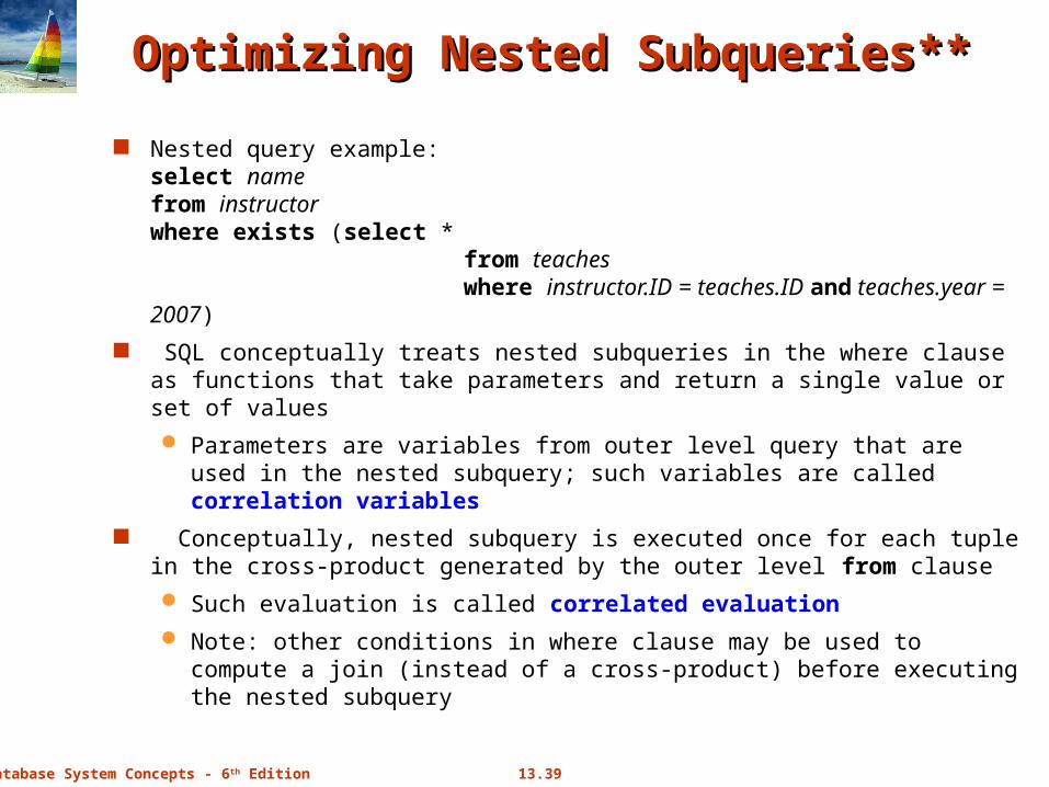
Nested query example:select namefrom instructorwhere exists (select *
from teaches where instructor.ID = teaches.ID and teaches.year =
2007)
SQL conceptually treats nested subqueries in the where clause as functions that take parameters and return a single value or set of values
Parameters are variables from outer level query that are used in the nested subquery; such variables are called correlation variables
Conceptually, nested subquery is executed once for each tuple in the cross-product generated by the outer level from clause
Such evaluation is called correlated evaluation
Note: other conditions in where clause may be used to compute a join (instead of a cross-product) before executing the nested subquery
13.40Database System Concepts - 6th Edition
Optimizing Nested Subqueries (Cont.)Optimizing Nested Subqueries (Cont.)
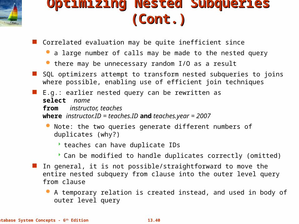
Correlated evaluation may be quite inefficient since
a large number of calls may be made to the nested query
there may be unnecessary random I/O as a result
SQL optimizers attempt to transform nested subqueries to joins where possible, enabling use of efficient join techniques
E.g.: earlier nested query can be rewritten as select namefrom instructor, teacheswhere instructor.ID = teaches.ID and teaches.year = 2007
Note: the two queries generate different numbers of duplicates (why?)
teaches can have duplicate IDs
Can be modified to handle duplicates correctly (omitted)
In general, it is not possible/straightforward to move the entire nested subquery from clause into the outer level query from clause
A temporary relation is created instead, and used in body of outer level query
13.41Database System Concepts - 6th Edition
Optimizing Nested Subqueries (Cont.)Optimizing Nested Subqueries (Cont.)
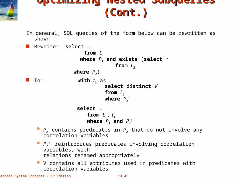
In general, SQL queries of the form below can be rewritten as shown Rewrite: select …
from L1
where P1 and exists (select * from L2
where P2)
To: with t1 as select distinct V from L2
where P21
select … from L1, t1 where P1 and P2
2
P21 contains predicates in P2 that do not involve any correlation
variables P2
2 reintroduces predicates involving correlation variables, with relations renamed appropriately
V contains all attributes used in predicates with correlation variables
13.42Database System Concepts - 6th Edition
Optimizing Nested Subqueries (Cont.)Optimizing Nested Subqueries (Cont.)
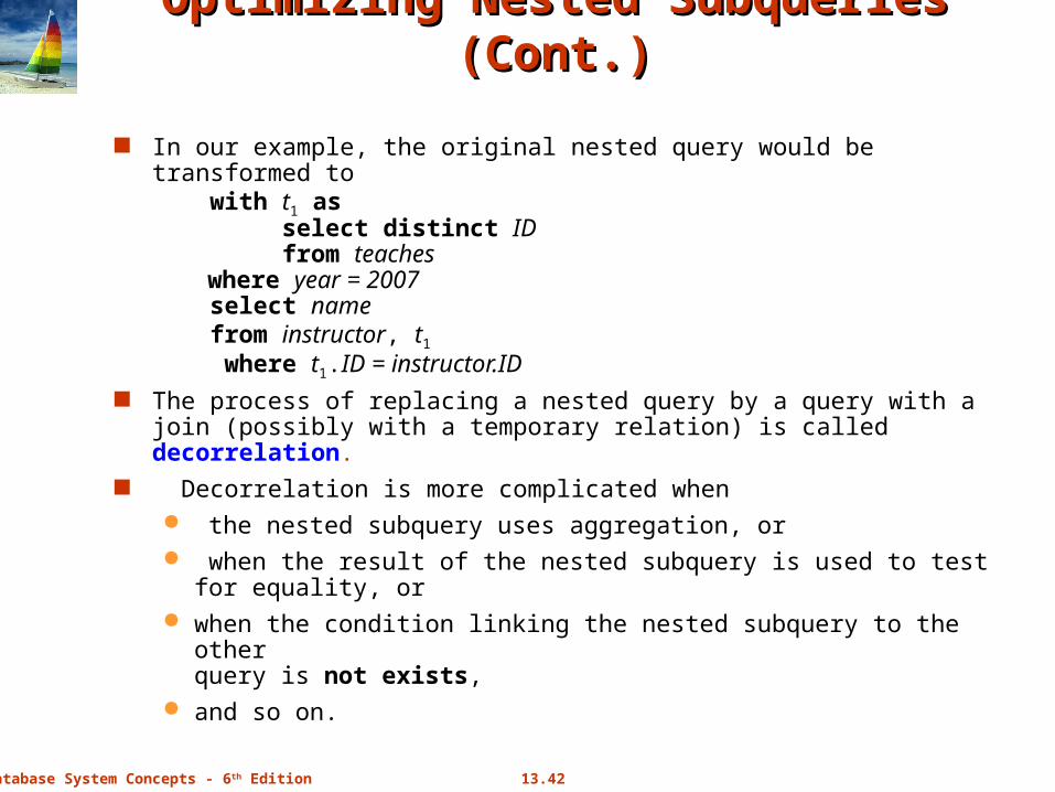
In our example, the original nested query would be transformed to with t1 as select distinct ID from teaches where year = 2007 select name from instructor, t1
where t1.ID = instructor.ID The process of replacing a nested query by a query with a join (possibly
with a temporary relation) is called decorrelation. Decorrelation is more complicated when
the nested subquery uses aggregation, or when the result of the nested subquery is used to test for equality, or when the condition linking the nested subquery to the other
query is not exists, and so on.
13.43Database System Concepts - 6th Edition
Materialized Views**Materialized Views**
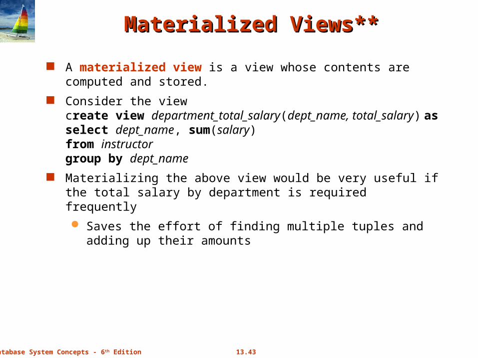
A materialized view is a view whose contents are computed and stored.
Consider the viewcreate view department_total_salary(dept_name, total_salary) asselect dept_name, sum(salary)from instructorgroup by dept_name
Materializing the above view would be very useful if the total salary by department is required frequently
Saves the effort of finding multiple tuples and adding up their amounts
13.44Database System Concepts - 6th Edition
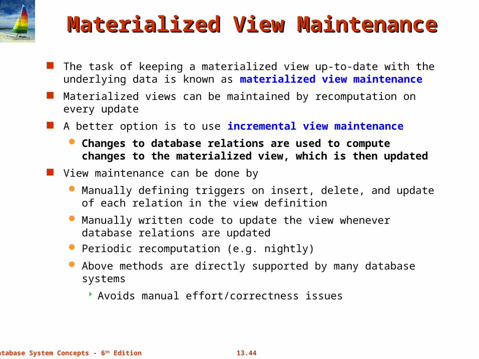
Materialized View MaintenanceMaterialized View Maintenance
The task of keeping a materialized view up-to-date with the underlying data is known as materialized view maintenance
Materialized views can be maintained by recomputation on every update
A better option is to use incremental view maintenance
Changes to database relations are used to compute changes to the materialized view, which is then updated
View maintenance can be done by
Manually defining triggers on insert, delete, and update of each relation in the view definition
Manually written code to update the view whenever database relations are updated
Periodic recomputation (e.g. nightly)
Above methods are directly supported by many database systems
Avoids manual effort/correctness issues
13.45Database System Concepts - 6th Edition
Incremental View MaintenanceIncremental View Maintenance
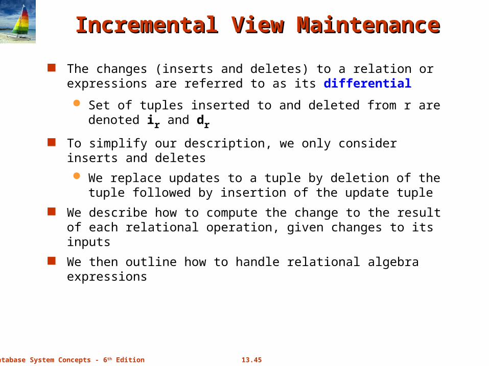
The changes (inserts and deletes) to a relation or expressions are referred to as its differential
Set of tuples inserted to and deleted from r are denoted ir and dr
To simplify our description, we only consider inserts and deletes
We replace updates to a tuple by deletion of the tuple followed by insertion of the update tuple
We describe how to compute the change to the result of each relational operation, given changes to its inputs
We then outline how to handle relational algebra expressions
13.46Database System Concepts - 6th Edition
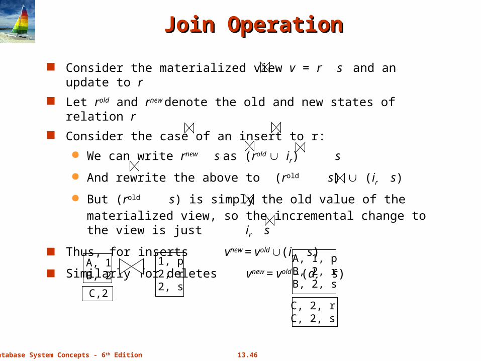
Join OperationJoin Operation
Consider the materialized view v = r s and an update to r
Let rold and rnew denote the old and new states of relation r
Consider the case of an insert to r:
We can write rnew s as (rold ir) s
And rewrite the above to (rold s) (ir s)
But (rold s) is simply the old value of the materialized view, so the
incremental change to the view is just ir s
Thus, for inserts vnew = vold (ir s)
Similarly for deletes vnew = vold – (dr s)
A, 1B, 2
1, p2, r2, s
A, 1, pB, 2, rB, 2, s
C,2C, 2, rC, 2, s
13.47Database System Concepts - 6th Edition
Selection and Projection OperationsSelection and Projection Operations
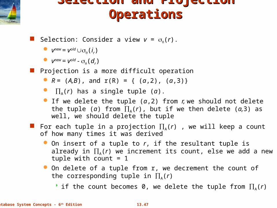
Selection: Consider a view v = (r).
vnew = vold (ir)
vnew = vold - (dr) Projection is a more difficult operation
R = (A,B), and r(R) = { (a,2), (a,3)} A(r) has a single tuple (a). If we delete the tuple (a,2) from r, we should not delete the tuple (a)
from A(r), but if we then delete (a,3) as well, we should delete the tuple
For each tuple in a projection A(r) , we will keep a count of how many times it was derived On insert of a tuple to r, if the resultant tuple is already in A(r) we
increment its count, else we add a new tuple with count = 1 On delete of a tuple from r, we decrement the count of the
corresponding tuple in A(r)
if the count becomes 0, we delete the tuple from A(r)
13.48Database System Concepts - 6th Edition
Aggregation OperationsAggregation Operations
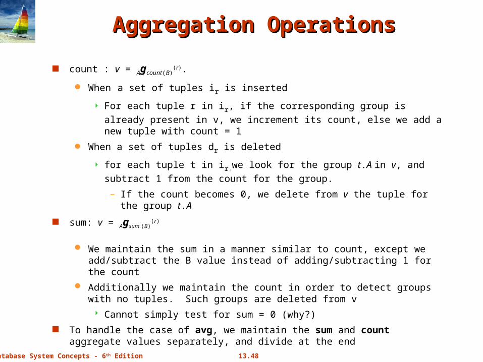
count : v = Agcount(B)(r).
When a set of tuples ir is inserted
For each tuple r in ir, if the corresponding group is already present in v,
we increment its count, else we add a new tuple with count = 1
When a set of tuples dr is deleted
for each tuple t in ir.we look for the group t.A in v, and subtract 1 from
the count for the group.
– If the count becomes 0, we delete from v the tuple for the group t.A
sum: v = Agsum (B)(r)
We maintain the sum in a manner similar to count, except we add/subtract the B value instead of adding/subtracting 1 for the count
Additionally we maintain the count in order to detect groups with no tuples. Such groups are deleted from v
Cannot simply test for sum = 0 (why?)
To handle the case of avg, we maintain the sum and count aggregate values separately, and divide at the end
13.49Database System Concepts - 6th Edition
Aggregate Operations (Cont.)Aggregate Operations (Cont.)
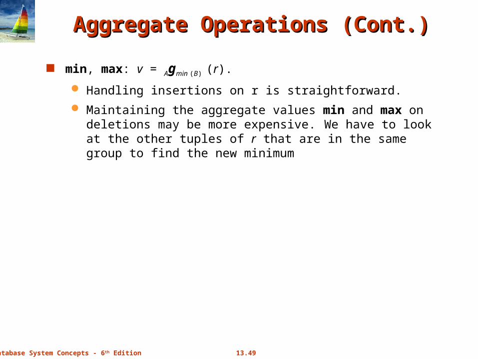
min, max: v = Agmin (B) (r).
Handling insertions on r is straightforward.
Maintaining the aggregate values min and max on deletions may be more expensive. We have to look at the other tuples of r that are in the same group to find the new minimum
13.50Database System Concepts - 6th Edition
Query Optimization and Materialized ViewsQuery Optimization and Materialized Views
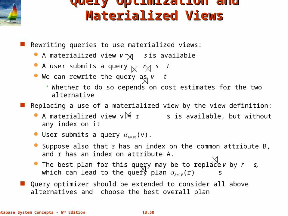
Rewriting queries to use materialized views:
A materialized view v = r s is available
A user submits a query r s t
We can rewrite the query as v t
Whether to do so depends on cost estimates for the two alternative
Replacing a use of a materialized view by the view definition:
A materialized view v = r s is available, but without any index on it
User submits a query A=10(v).
Suppose also that s has an index on the common attribute B, and r has an index on attribute A.
The best plan for this query may be to replace v by r s, which can lead to the query plan A=10(r) s
Query optimizer should be extended to consider all above alternatives and choose the best overall plan
13.51Database System Concepts - 6th Edition
Materialized View SelectionMaterialized View Selection
Materialized view selection: “What is the best set of views to materialize?”.
Index selection: “what is the best set of indices to create”
closely related, to materialized view selection but simpler
Materialized view selection and index selection based on typical system workload (queries and updates)
Typical goal: minimize time to execute workload , subject to constraints on space and time taken for some critical queries/updates
One of the steps in database tuning
more on tuning in later chapters
Commercial database systems provide tools (called “tuning assistants” or “wizards”) to help the database administrator choose what indices and materialized views to create
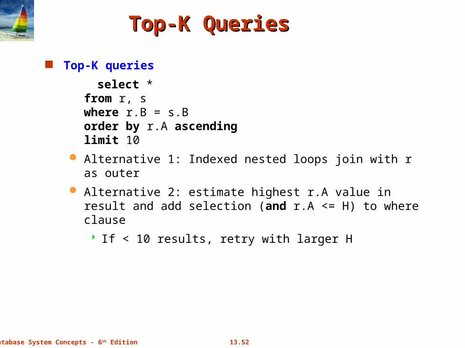
13.52Database System Concepts - 6th Edition
Top-K QueriesTop-K Queries
Top-K queries
select * from r, swhere r.B = s.Border by r.A ascendinglimit 10
Alternative 1: Indexed nested loops join with r as outer
Alternative 2: estimate highest r.A value in result and add selection (and r.A <= H) to where clause
If < 10 results, retry with larger H
13.53Database System Concepts - 6th Edition
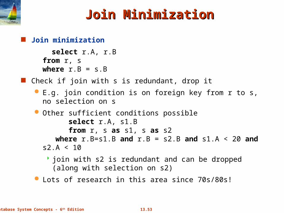
Join MinimizationJoin Minimization
Join minimization
select r.A, r.B from r, swhere r.B = s.B
Check if join with s is redundant, drop it
E.g. join condition is on foreign key from r to s, no selection on s
Other sufficient conditions possibleselect r.A, s1.B from r, s as s1, s as s2
where r.B=s1.B and r.B = s2.B and s1.A < 20 and s2.A < 10
join with s2 is redundant and can be dropped (along with selection on s2)
Lots of research in this area since 70s/80s!