Embed Size (px)
Citation preview
2 - 1 Convexity and Duality P. Parrilo and S. Lall, CDC 2003 2003.12.07.03
2. Convexity and Duality
• Convex sets and functions
• Convex optimization problems
• Standard problems: LP and SDP
• Feasibility problems
• Algorithms
• Certificates and separating hyperplanes
• Duality and geometry
• Examples: LP and and SDP
• Theorems of alternatives
2 - 2 Convexity and Duality P. Parrilo and S. Lall, CDC 2003 2003.12.07.03
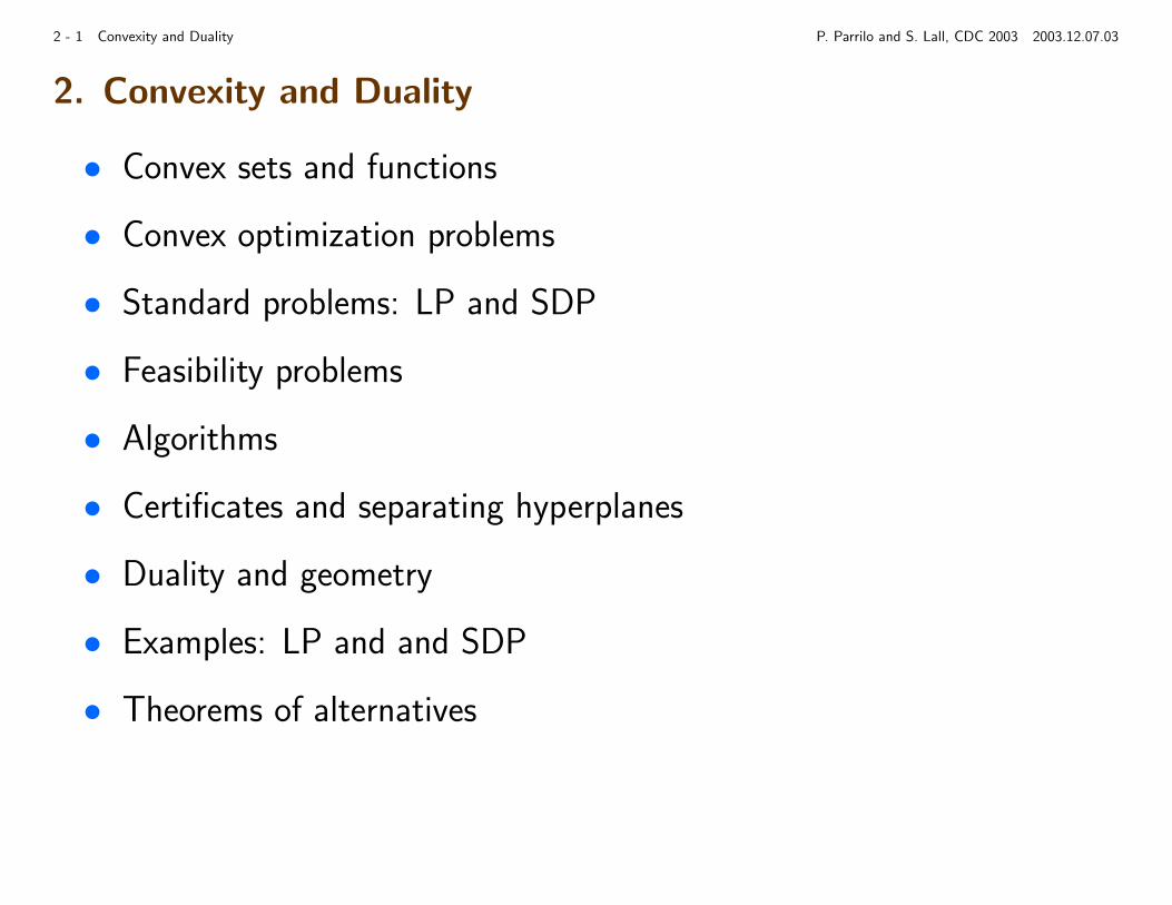
Basic Nomenclature
A set S ⊂ Rn is called
• affine if x, y ∈ S implies θx + (1 − θ)y ∈ S for all θ ∈ R; i.e., theline through x, y is contained in S
• convex if x, y ∈ S implies θx + (1 − θ)y ∈ S for all θ ∈ [0, 1]; i.e.,the line segment between x and y is contained in S.
• a convex cone if x, y ∈ S implies λx + µy ∈ S for all λ, µ ≥ 0; i.e.,the pie slice between x and y is contained in S.
A function f : Rn→ R is called
• affine if f (θx + (1 − θ)y) = θf (x) + (1 − θ)f (y) for all θ ∈ R andx, y ∈ Rn; i.e., f is equals a linear function plus a constant f = Ax+b
• convex if f(θx + (1 − θ)y
)≤ θf (x) + (1 − θ)f (y) for all θ ∈ [0, 1]
and x, y ∈ Rn
2 - 3 Convexity and Duality P. Parrilo and S. Lall, CDC 2003 2003.12.07.03
Properties of Convex Functions
• f1 + f2 is convex if f1 and f2 are
• f (x) = max{f1(x), f2(x)} is convex if f1 and f2 are
• g(x) = supy f (x, y) is convex if f (x, y) is convex in x for each y
• convex functions are continuous on the interior of their domain
• f (Ax + b) is convex if f is
• Af (x) + b is convex if f is
• g(x) = infy f (x, y) is convex if f (x, y) is jointly convex
• the α−sublevel set
{x ∈ Rn | f (x) ≤ α }
is convex if f is convex; (the converse is not true)
2 - 4 Convexity and Duality P. Parrilo and S. Lall, CDC 2003 2003.12.07.03
Convex Optimization Problems
minimize f0(x)
subject to fi(x) ≤ 0 for all i = 1, . . . ,m
hi(x) = 0 for all i = 1, . . . , p
This problem is called a convex program if
• the objective function f0 is convex
• the inequality constraints fi are convex
• the equality constraints hi are affine
2 - 5 Convexity and Duality P. Parrilo and S. Lall, CDC 2003 2003.12.07.03
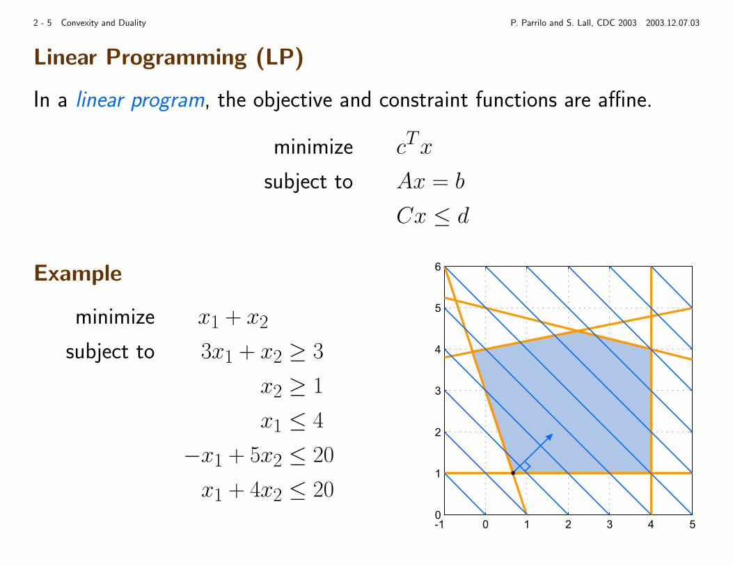
Linear Programming (LP)
In a linear program, the objective and constraint functions are affine.
minimize cTx
subject to Ax = b
Cx ≤ d
Example
minimize x1 + x2
subject to 3x1 + x2 ≥ 3
x2 ≥ 1
x1 ≤ 4
−x1 + 5x2 ≤ 20
x1 + 4x2 ≤ 20
2 - 6 Convexity and Duality P. Parrilo and S. Lall, CDC 2003 2003.12.07.03
Linear Programming
Every linear program may be written in the standard primal form
minimize cTx
subject to Ax = b
x ≥ 0
Here x ∈ Rn, and x ≥ 0 means xi ≥ 0 for all i
• The nonnegative orthant{x ∈ Rn | x ≥ 0
}is a convex cone.
• This convex cone defines the partial ordering ≥ on Rn
• Geometrically, the feasible set is the intersection of an affine set witha convex cone.
2 - 7 Convexity and Duality P. Parrilo and S. Lall, CDC 2003 2003.12.07.03
Semidefinite Programming
minimize traceCX
subject to traceAiX = bi for all i = 1, . . . ,m
X º 0
• The variable X is in the set of n× n symmetric matrices
Sn ={A ∈ Rn×n | A = AT
}
• X º 0 means X is positive semidefinite
• As for LP, the feasible set is the intersection of an affine set with aconvex cone, in this case the positive semidefinite cone
{X ∈ Sn | X º 0
}
Hence the feasible set is convex.
2 - 8 Convexity and Duality P. Parrilo and S. Lall, CDC 2003 2003.12.07.03
SDPs with Explicit Variables
We can also explicitly parametrize the affine set to give
minimize cTx
subject to F0 + x1F1 + x2F2 + · · · + xnFn ¹ 0
where F0, F1, . . . , Fn are symmetric matrices.
The inequality constraint is called a linear matrix inequality; e.g.,x1 − 3 x1 + x2 −1x1 + x2 x2 − 4 0−1 0 x1
¹ 0
which is equivalent to−3 0 −10 −4 0−1 0 0
+ x1
1 1 01 0 00 0 1
+ x2
0 1 01 1 00 0 0
¹ 0
2 - 9 Convexity and Duality P. Parrilo and S. Lall, CDC 2003 2003.12.07.03
The Feasible Set is Semialgebraic
The (basic closed) semialgebraic set defined by polynomials f1, . . . , fm is{x ∈ Rn | fi(x) ≥ 0 for all i = 1, . . . ,m
}
The feasible set of an SDP is a semialgebraic set.
Because a matrix A Â 0 if and only if
det(Ak) > 0 for k = 1, . . . , n
where Ak is the submatrix of A consisting of the first k rows and columns.
2 - 10 Convexity and Duality P. Parrilo and S. Lall, CDC 2003 2003.12.07.03
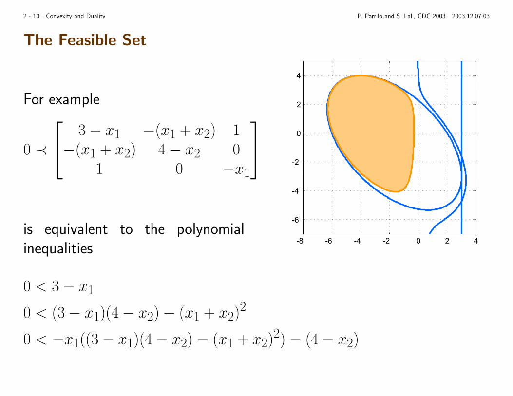
The Feasible Set
For example
0 ≺
3− x1 −(x1 + x2) 1−(x1 + x2) 4− x2 0
1 0 −x1
is equivalent to the polynomialinequalities
0 < 3− x1
0 < (3− x1)(4− x2)− (x1 + x2)2
0 < −x1((3− x1)(4− x2)− (x1 + x2)2)− (4− x2)
2 - 11 Convexity and Duality P. Parrilo and S. Lall, CDC 2003 2003.12.07.03
Feasible Sets of SDP
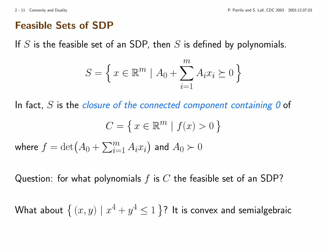
If S is the feasible set of an SDP, then S is defined by polynomials.
S ={x ∈ Rm | A0 +
m∑
i=1
Aixi º 0}
In fact, S is the closure of the connected component containing 0 of
C ={x ∈ Rm | f (x) > 0
}
where f = det(A0 +
∑mi=1Aixi
)and A0 Â 0
Question: for what polynomials f is C the feasible set of an SDP?
What about{
(x, y) | x4 + y4 ≤ 1}
? It is convex and semialgebraic
−1.5 −1 −0.5 0 0.5 1 1.5−1.5
−1
−0.5
0
0.5
1
1.5
2 - 12 Convexity and Duality P. Parrilo and S. Lall, CDC 2003 2003.12.07.03
A Necessary Condition
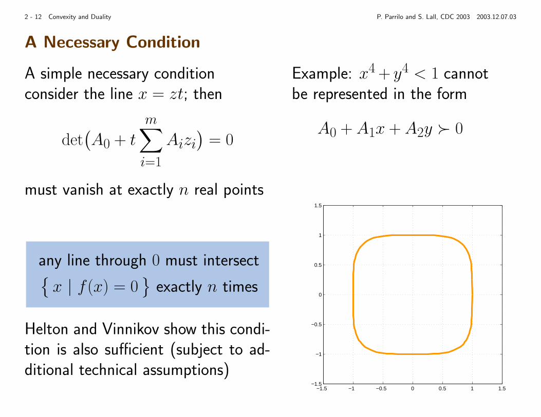
A simple necessary conditionconsider the line x = zt; then
det(A0 + t
m∑
i=1
Aizi)
= 0
must vanish at exactly n real points
any line through 0 must intersect{x | f (x) = 0
}exactly n times
Helton and Vinnikov show this condi-tion is also sufficient (subject to ad-ditional technical assumptions)
Example: x4 + y4 < 1 cannotbe represented in the form
A0 + A1x + A2y  0
−1.5 −1 −0.5 0 0.5 1 1.5−1.5
−1
−0.5
0
0.5
1
1.5
2 - 13 Convexity and Duality P. Parrilo and S. Lall, CDC 2003 2003.12.07.03
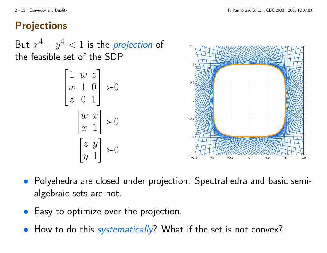
Projections
But x4 + y4 < 1 is the projection ofthe feasible set of the SDP
1 w zw 1 0z 0 1
Â0
[w xx 1
]Â0
[z yy 1
]Â0
• Polyehedra are closed under projection. Spectrahedra and basic semi-algebraic sets are not.
• Easy to optimize over the projection.
• How to do this systematically? What if the set is not convex?
2 - 14 Convexity and Duality P. Parrilo and S. Lall, CDC 2003 2003.12.07.03
Convex Optimization Problems
For a convex optimization problem, the feasible set
S ={x ∈ Rn | fi(x) ≤ 0 and hj(x) = 0 for all i, j
}
is convex. So we can write the problem as
minimize f0(x)
subject to x ∈ S
This approach emphasizes the geometry of the problem.
For a convex optimization problem, any local minimum is also a globalminimum.
2 - 15 Convexity and Duality P. Parrilo and S. Lall, CDC 2003 2003.12.07.03
Feasibility Problems
We are also interested in feasibility problems as follows. Does there existx ∈ Rn which satisfies
fi(x) ≤ 0 for all i = 1, . . . ,m
hi(x) = 0 for all i = 1, . . . , p
If there does not exist such an x, the problem is described as infeasible.
2 - 16 Convexity and Duality P. Parrilo and S. Lall, CDC 2003 2003.12.07.03
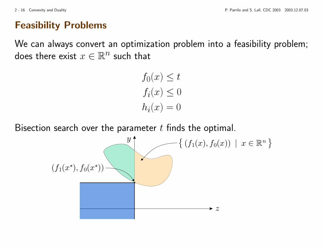
Feasibility Problems
We can always convert an optimization problem into a feasibility problem;does there exist x ∈ Rn such that
f0(x) ≤ t
fi(x) ≤ 0
hi(x) = 0
Bisection search over the parameter t finds the optimal.
(f1(x?); f0(x?))
z
y è
(f1(x); f0(x)) j x 2 Rné
2 - 17 Convexity and Duality P. Parrilo and S. Lall, CDC 2003 2003.12.07.03
Feasibility Problems
Conversely, we can convert feasibility problems into optimization problems.
e.g. the feasibility problem of finding x such that
fi(x) ≤ 0 for all i = 1, . . . ,m
can be solved as
minimize y
subject to fi(x) ≤ y for all i = 1, . . . ,m
where there are n + 1 variables x ∈ Rn and y ∈ R
This technique may be used to find an initial feasible point for optimizationalgorithms
2 - 18 Convexity and Duality P. Parrilo and S. Lall, CDC 2003 2003.12.07.03
Algorithms
For convex optimization problems, there are several good algorithms
• interior-point algorithms work well in theory and practice
• for certain classes of problems, (e.g. LP and SDP) there is a worst-casetime-complexity bound
• conversely, some convex optimization problems are known to be NP-hard
• problems are specified either in standard form, for LPs and SDPs, orvia an oracle
2 - 19 Convexity and Duality P. Parrilo and S. Lall, CDC 2003 2003.12.07.03
Certificates
Consider the feasibility problem
Does there exist x ∈ Rn which satisfies
fi(x) ≤ 0 for all i = 1, . . . ,m
hi(x) = 0 for all i = 1, . . . , p
There is a fundamental asymmetry between establishing that
• There exists at least one feasible x
• The problem is infeasible
To show existence, one needs a feasible point x ∈ Rn.
To show emptiness, one needs a a certificate of infeasibility; a mathematicalproof that the problem is infeasible.
2 - 20 Convexity and Duality P. Parrilo and S. Lall, CDC 2003 2003.12.07.03
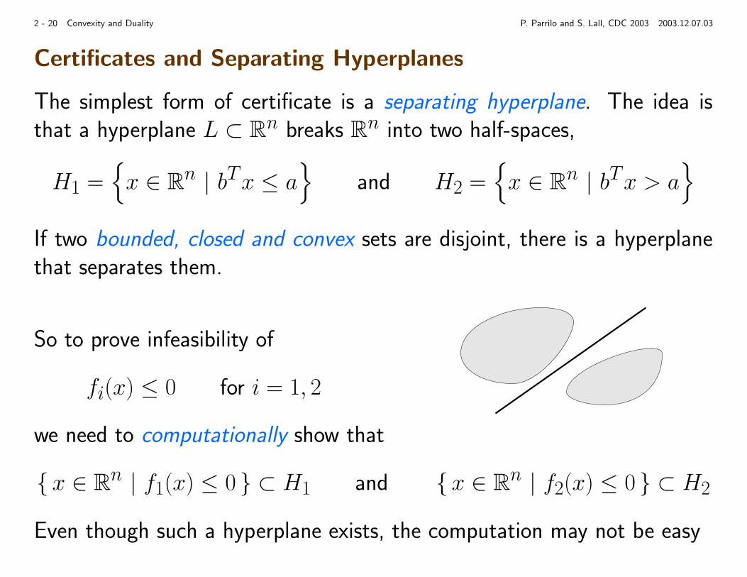
Certificates and Separating Hyperplanes
The simplest form of certificate is a separating hyperplane. The idea isthat a hyperplane L ⊂ Rn breaks Rn into two half-spaces,
H1 ={x ∈ Rn | bTx ≤ a
}and H2 =
{x ∈ Rn | bTx > a
}
If two bounded, closed and convex sets are disjoint, there is a hyperplanethat separates them.
So to prove infeasibility of
fi(x) ≤ 0 for i = 1, 2
we need to computationally show that
{x ∈ Rn | f1(x) ≤ 0 } ⊂ H1 and {x ∈ Rn | f2(x) ≤ 0 } ⊂ H2
Even though such a hyperplane exists, the computation may not be easy
2 - 21 Convexity and Duality P. Parrilo and S. Lall, CDC 2003 2003.12.07.03
Duality
We’d like to solve
minimize f0(x)
subject to fi(x) ≤ 0 for all i = 1, . . . ,m
hi(x) = 0 for all i = 1, . . . , p
define the Lagrangian for x ∈ Rn, λ ∈ Rm and ν ∈ Rp by
L(x, λ, ν) = f0(x) +
m∑
i=1
λifi(x) +
p∑
i=1
νihi(x)
and the Lagrange dual function
g(λ, ν) = infx∈Rn
L(x, λ, ν)
We allow g(λ, ν) = −∞ when there is no finite infimum
2 - 22 Convexity and Duality P. Parrilo and S. Lall, CDC 2003 2003.12.07.03
Duality
The dual problem is
maximize g(λ, ν)
subject to λ ≥ 0
We call λ, ν dual feasible if λ ≥ 0 and g(λ, ν) is finite.
• The dual function g is always concave, even if the primal problem isnot convex
2 - 23 Convexity and Duality P. Parrilo and S. Lall, CDC 2003 2003.12.07.03
Weak Duality
For any primal feasible x and dual feasible λ, ν we have
g(λ, ν) ≤ f0(x)
because
g(λ, ν) ≤ f0(x) +
m∑
i=1
λifi(x) +
p∑
i=1
νihi(x)
≤ f0(x)
• A feasible λ, ν provides a certificate that the primal optimal is greaterthan g(λ, ν)
• many interior-point methods simultaneously optimize the primal andthe dual problem; when f0(x) − g(λ, ν) ≤ ε we know that x isε−suboptimal
2 - 24 Convexity and Duality P. Parrilo and S. Lall, CDC 2003 2003.12.07.03
Strong Duality
• p? is the optimal value of the primal problem,
• d? is the optimal value of the dual problem
Weak duality means p? ≥ d?
If p? = d? we say strong duality holds. Equivalently, we say the duality gapp? − d? is zero.
Constraint qualifications give sufficient conditions for strong duality.
An example is Slater’s condition; strong duality holds if the primal problemis convex and strictly feasible.
2 - 25 Convexity and Duality P. Parrilo and S. Lall, CDC 2003 2003.12.07.03
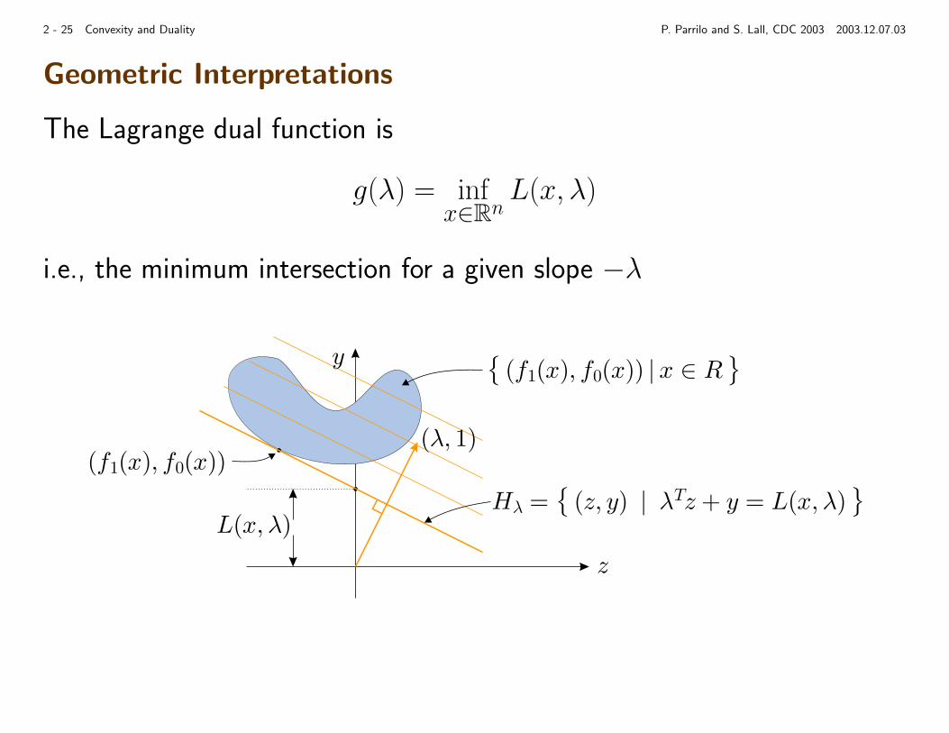
Geometric Interpretations
The Lagrange dual function is
g(λ) = infx∈Rn
L(x, λ)
i.e., the minimum intersection for a given slope −λ
è
(f1(x); f0(x)) j x 2 Ré
(õ; 1)(f1(x); f0(x))
Hõ =è
(z; y) j õTz + y = L(x;õ)é
L(x;õ)
z
y
2 - 26 Convexity and Duality P. Parrilo and S. Lall, CDC 2003 2003.12.07.03
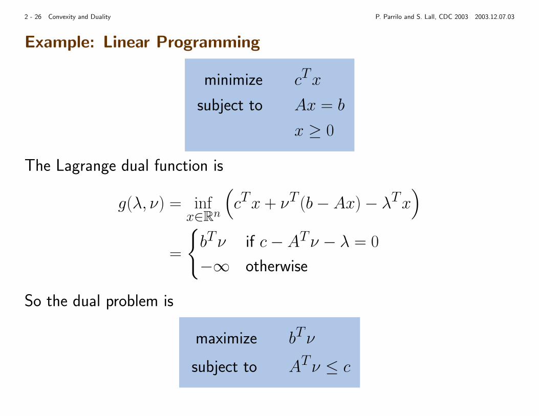
Example: Linear Programming
minimize cTx
subject to Ax = b
x ≥ 0
The Lagrange dual function is
g(λ, ν) = infx∈Rn
(cTx + νT (b− Ax)− λTx
)
=
{bTν if c− ATν − λ = 0
−∞ otherwise
So the dual problem is
maximize bTν
subject to ATν ≤ c
2 - 27 Convexity and Duality P. Parrilo and S. Lall, CDC 2003 2003.12.07.03
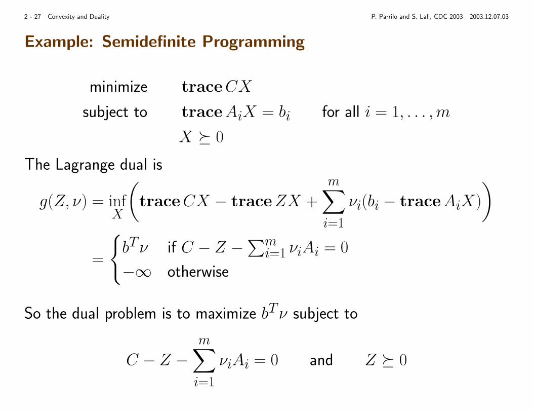
Example: Semidefinite Programming
minimize traceCX
subject to traceAiX = bi for all i = 1, . . . ,m
X º 0
The Lagrange dual is
g(Z, ν) = infX
(traceCX − traceZX +
m∑
i=1
νi(bi − traceAiX)
)
=
{bTν if C − Z −∑m
i=1 νiAi = 0
−∞ otherwise
So the dual problem is to maximize bTν subject to
C − Z −m∑
i=1
νiAi = 0 and Z º 0
2 - 28 Convexity and Duality P. Parrilo and S. Lall, CDC 2003 2003.12.07.03
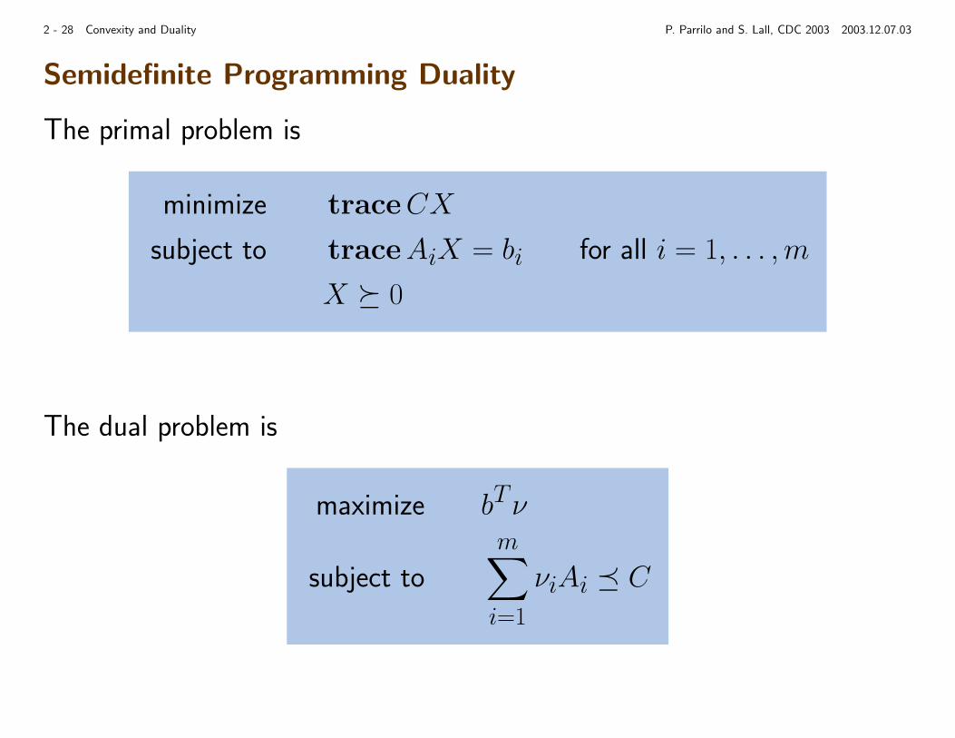
Semidefinite Programming Duality
The primal problem is
minimize traceCX
subject to traceAiX = bi for all i = 1, . . . ,m
X º 0
The dual problem is
maximize bTν
subject tom∑
i=1
νiAi ¹ C
2 - 29 Convexity and Duality P. Parrilo and S. Lall, CDC 2003 2003.12.07.03
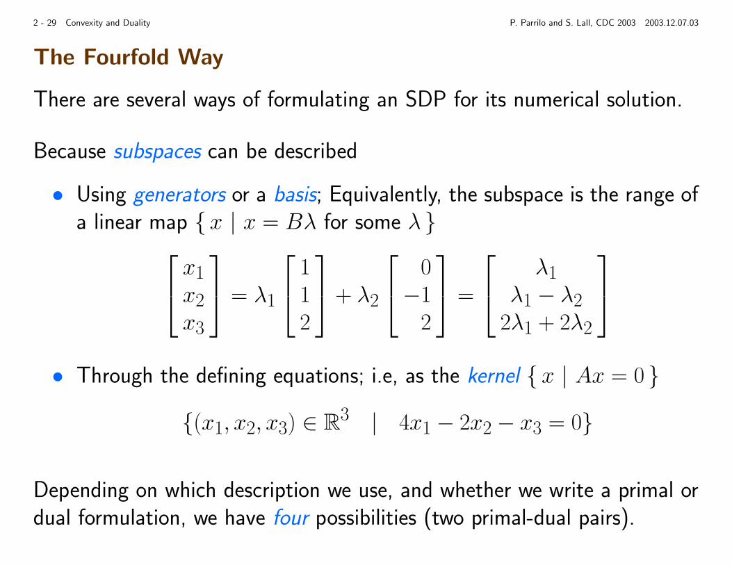
The Fourfold Way
There are several ways of formulating an SDP for its numerical solution.
Because subspaces can be described
• Using generators or a basis; Equivalently, the subspace is the range ofa linear map {x | x = Bλ for some λ }
x1x2x3
= λ1
112
+ λ2
0−1
2
=
λ1λ1 − λ2
2λ1 + 2λ2
• Through the defining equations; i.e, as the kernel {x | Ax = 0 }
{(x1, x2, x3) ∈ R3 | 4x1 − 2x2 − x3 = 0}
Depending on which description we use, and whether we write a primal ordual formulation, we have four possibilities (two primal-dual pairs).
2 - 30 Convexity and Duality P. Parrilo and S. Lall, CDC 2003 2003.12.07.03
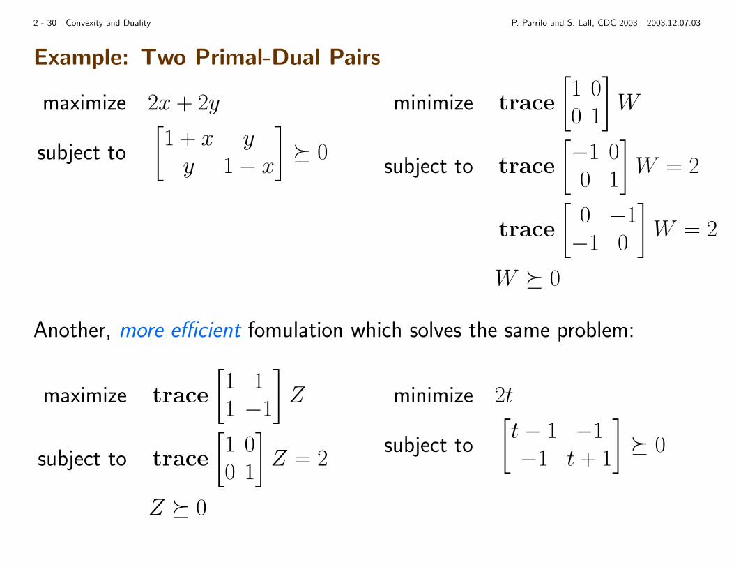
Example: Two Primal-Dual Pairs
maximize 2x + 2y
subject to
[1 + x yy 1− x
]º 0
minimize trace
[1 00 1
]W
subject to trace
[−1 00 1
]W = 2
trace
[0 −1−1 0
]W = 2
W º 0
Another, more efficient fomulation which solves the same problem:
maximize trace
[1 11 −1
]Z
subject to trace
[1 00 1
]Z = 2
Z º 0
minimize 2t
subject to
[t− 1 −1−1 t + 1
]º 0
2 - 31 Convexity and Duality P. Parrilo and S. Lall, CDC 2003 2003.12.07.03
Duality
• Duality has many interpretations; via economics, game-theory, geom-etry.
• e.g., one may interpret Lagrange multipliers as a price for violatingconstraints, which may correspond to resource limits or capacity con-straints.
• Often physical problems associate specific meaning to certain Lagrangemultipliers, e.g. pressure, momentum, force can all be viewed as La-grange multipliers
m
k
2 - 32 Convexity and Duality P. Parrilo and S. Lall, CDC 2003 2003.12.07.03
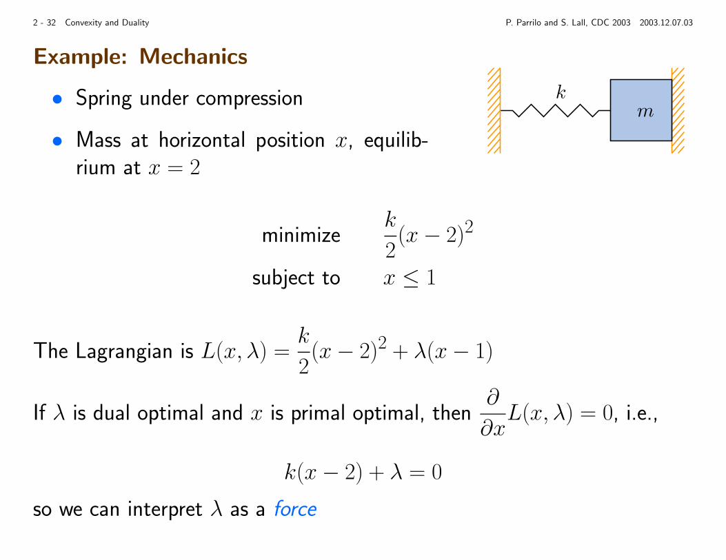
Example: Mechanics
• Spring under compression
• Mass at horizontal position x, equilib-rium at x = 2
minimizek
2(x− 2)2
subject to x ≤ 1
The Lagrangian is L(x, λ) =k
2(x− 2)2 + λ(x− 1)
If λ is dual optimal and x is primal optimal, then∂
∂xL(x, λ) = 0, i.e.,
k(x− 2) + λ = 0
so we can interpret λ as a force
2 - 33 Convexity and Duality P. Parrilo and S. Lall, CDC 2003 2003.12.07.03
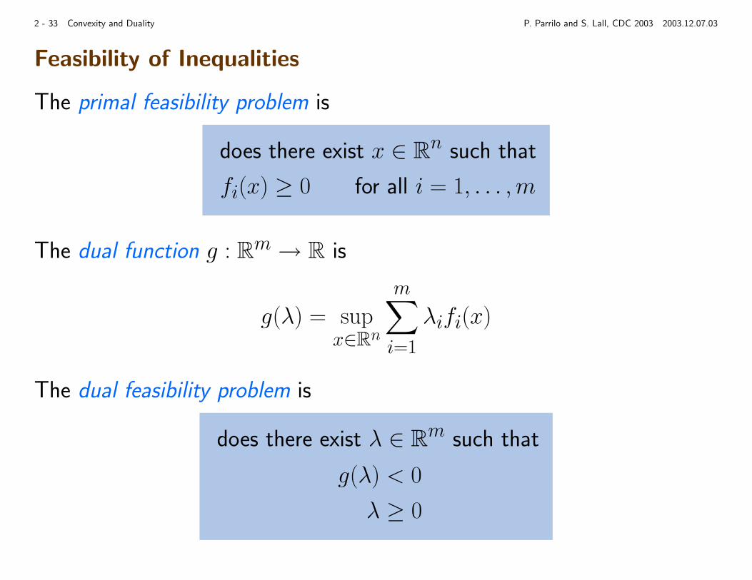
Feasibility of Inequalities
The primal feasibility problem is
does there exist x ∈ Rn such that
fi(x) ≥ 0 for all i = 1, . . . ,m
The dual function g : Rm→ R is
g(λ) = supx∈Rn
m∑
i=1
λifi(x)
The dual feasibility problem is
does there exist λ ∈ Rm such that
g(λ) < 0
λ ≥ 0

2 - 34 Convexity and Duality P. Parrilo and S. Lall, CDC 2003 2003.12.07.03
Theorem of Alternatives
If the dual problem is feasible, then the primal problem is infeasible.
Proof
Suppose the primal problem is feasible, and let x̃ be a feasible point. Then
g(λ) = supx∈Rn
m∑
i=1
λifi(x)
≥m∑
i=1
λifi(x̃) for all λ ∈ Rm
and so g(λ) ≥ 0 for all λ ≥ 0.
2 - 35 Convexity and Duality P. Parrilo and S. Lall, CDC 2003 2003.12.07.03
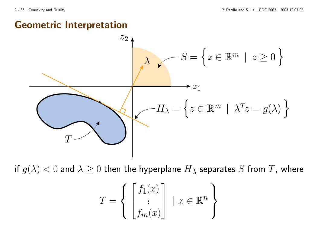
Geometric Interpretation
õ
z1
z2
Hõ =n
z 2 Rm j õTz = g(õ)
o
S =n
z 2 Rm j z õ 0
o
T
if g(λ) < 0 and λ ≥ 0 then the hyperplane Hλ separates S from T , where
T =
f1(x)
...fm(x)
| x ∈ Rn
2 - 36 Convexity and Duality P. Parrilo and S. Lall, CDC 2003 2003.12.07.03
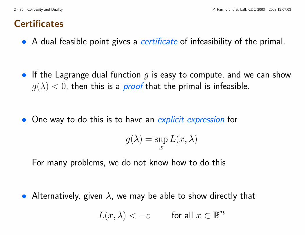
Certificates
• A dual feasible point gives a certificate of infeasibility of the primal.
• If the Lagrange dual function g is easy to compute, and we can showg(λ) < 0, then this is a proof that the primal is infeasible.
• One way to do this is to have an explicit expression for
g(λ) = supxL(x, λ)
For many problems, we do not know how to do this
• Alternatively, given λ, we may be able to show directly that
L(x, λ) < −ε for all x ∈ Rn
2 - 37 Convexity and Duality P. Parrilo and S. Lall, CDC 2003 2003.12.07.03
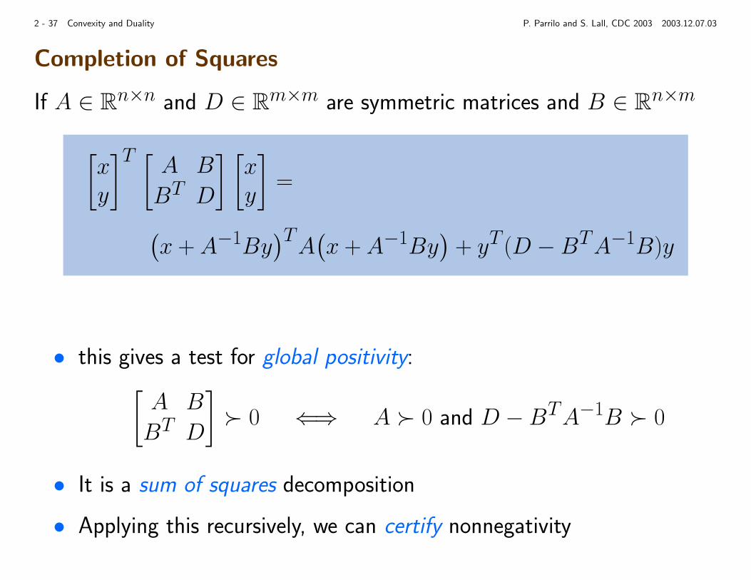
Completion of Squares
If A ∈ Rn×n and D ∈ Rm×m are symmetric matrices and B ∈ Rn×m
[xy
]T [ A B
BT D
] [xy
]=
(x + A−1By
)TA(x + A−1By
)+ yT (D −BTA−1B)y
• this gives a test for global positivity:[A B
BT D
]Â 0 ⇐⇒ A Â 0 and D −BTA−1B Â 0
• It is a sum of squares decomposition
• Applying this recursively, we can certify nonnegativity
2 - 38 Convexity and Duality P. Parrilo and S. Lall, CDC 2003 2003.12.07.03
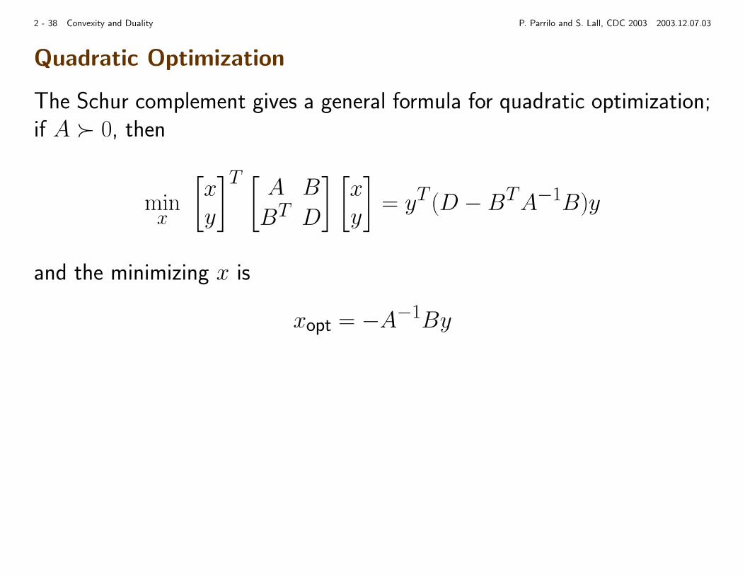
Quadratic Optimization
The Schur complement gives a general formula for quadratic optimization;if A Â 0, then
minx
[xy
]T [ A B
BT D
] [xy
]= yT (D −BTA−1B)y
and the minimizing x is
xopt = −A−1By