Embed Size (px)
Citation preview
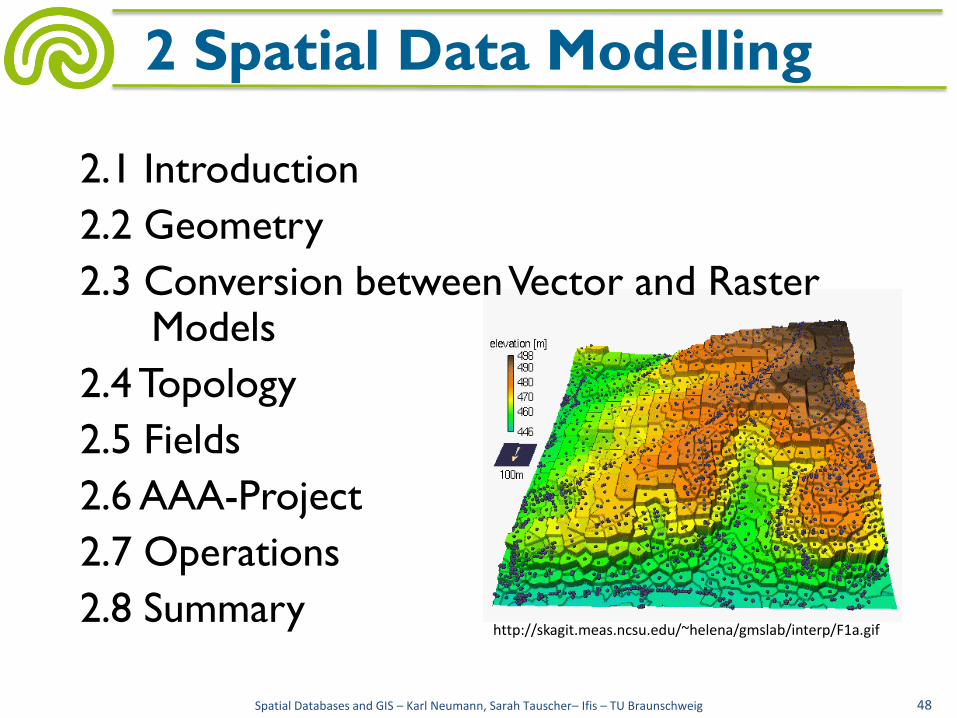
2.1 Introduction
2.2 Geometry
2.3 Conversion between Vector and Raster Models
2.4 Topology
2.5 Fields
2.6 AAA-Project
2.7 Operations
2.8 Summary
Spatial Databases and GIS – Karl Neumann, Sarah Tauscher– Ifis – TU Braunschweig 48
2 Spatial Data Modelling
http://skagit.meas.ncsu.edu/~helena/gmslab/interp/F1a.gif
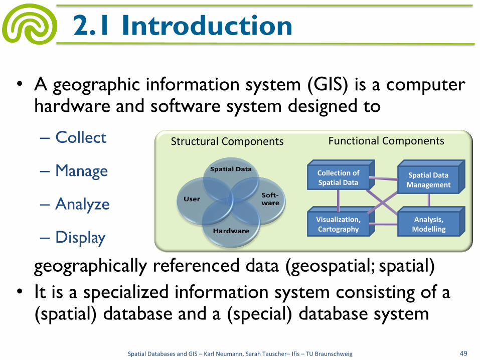
• A geographic information system (GIS) is a computer hardware and software system designed to
– Collect
– Manage
– Analyze
– Display
geographically referenced data (geospatial; spatial)
• It is a specialized information system consisting of a (spatial) database and a (special) database system
Spatial Databases and GIS – Karl Neumann, Sarah Tauscher– Ifis – TU Braunschweig 49
2.1 Introduction
Visualization, Cartography
Spatial Data Management
Collection of Spatial Data
Analysis, Modelling
Functional Components Structural Components
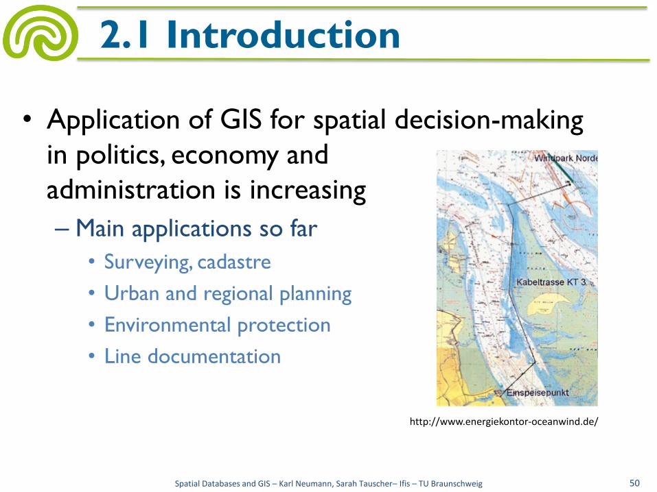
• Application of GIS for spatial decision-making
in politics, economy and
administration is increasing
– Main applications so far
• Surveying, cadastre
• Urban and regional planning
• Environmental protection
• Line documentation
Spatial Databases and GIS – Karl Neumann, Sarah Tauscher– Ifis – TU Braunschweig 50
2.1 Introduction
http://www.energiekontor-oceanwind.de/
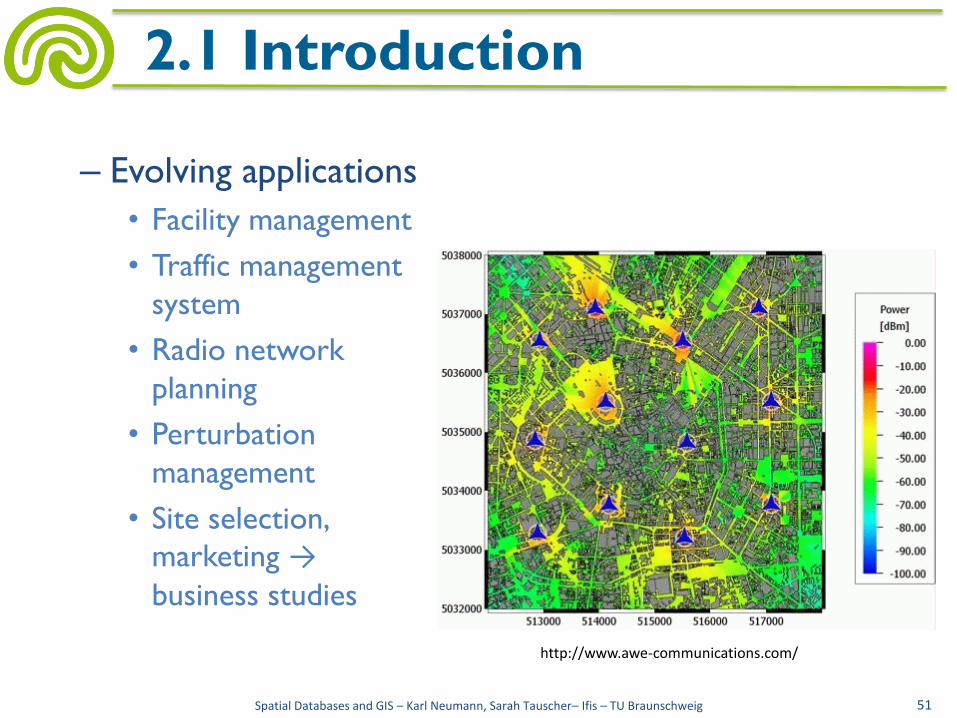
– Evolving applications
• Facility management
• Traffic management
system
• Radio network
planning
• Perturbation
management
• Site selection,
marketing →
business studies
Spatial Databases and GIS – Karl Neumann, Sarah Tauscher– Ifis – TU Braunschweig 51
2.1 Introduction
http://www.awe-communications.com/
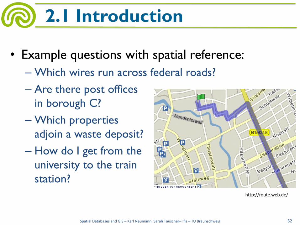
• Example questions with spatial reference:
– Which wires run across federal roads?
– Are there post offices
in borough C?
– Which properties
adjoin a waste deposit?
– How do I get from the
university to the train
station?
Spatial Databases and GIS – Karl Neumann, Sarah Tauscher– Ifis – TU Braunschweig 52
2.1 Introduction
http://route.web.de/
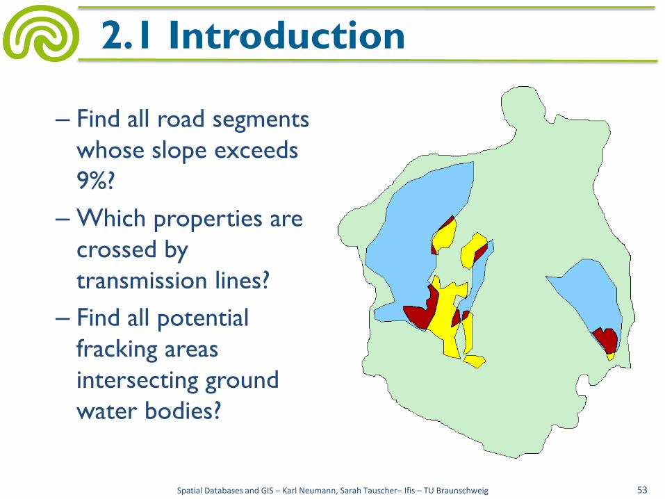
– Find all road segments
whose slope exceeds
9%?
– Which properties are
crossed by
transmission lines?
– Find all potential
fracking areas
intersecting ground
water bodies?
Spatial Databases and GIS – Karl Neumann, Sarah Tauscher– Ifis – TU Braunschweig 53
2.1 Introduction
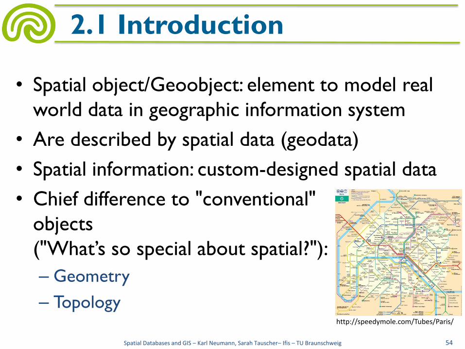
• Spatial object/Geoobject: element to model real
world data in geographic information system
• Are described by spatial data (geodata)
• Spatial information: custom-designed spatial data
• Chief difference to "conventional"
objects
("What’s so special about spatial?"):
– Geometry
– Topology
Spatial Databases and GIS – Karl Neumann, Sarah Tauscher– Ifis – TU Braunschweig 54
2.1 Introduction
http://speedymole.com/Tubes/Paris/
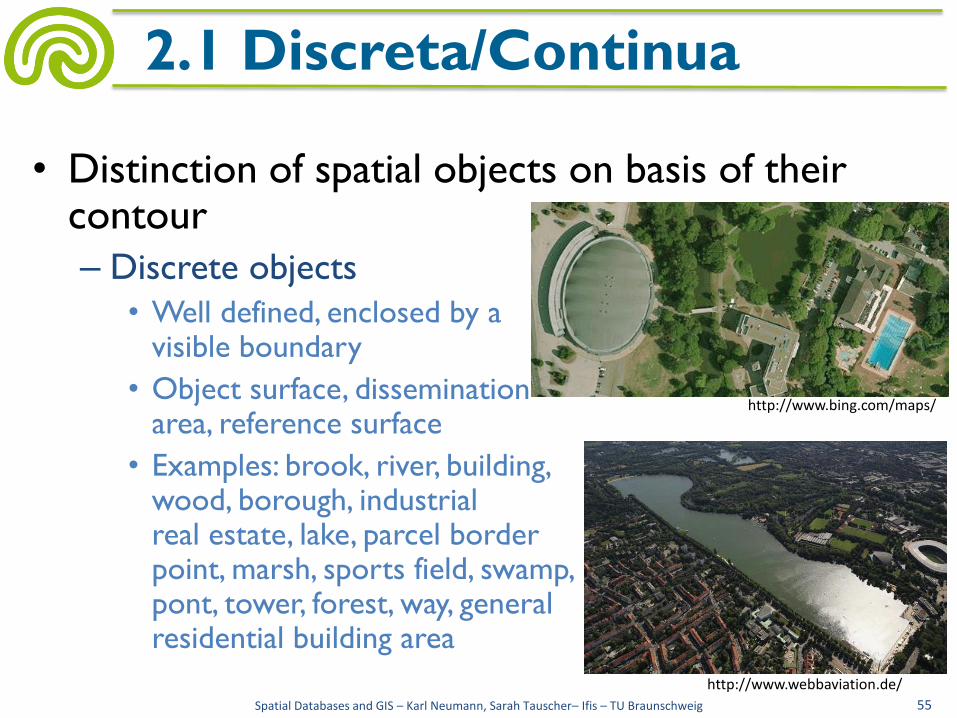
• Distinction of spatial objects on basis of their contour
– Discrete objects
• Well defined, enclosed by a visible boundary
• Object surface, dissemination area, reference surface
• Examples: brook, river, building, wood, borough, industrial real estate, lake, parcel border point, marsh, sports field, swamp, pont, tower, forest, way, general residential building area
Spatial Databases and GIS – Karl Neumann, Sarah Tauscher– Ifis – TU Braunschweig 55
2.1 Discreta/Continua
http://www.bing.com/maps/
http://www.webbaviation.de/
Spatial Databases and GIS – Karl Neumann, Sarah Tauscher– Ifis – TU Braunschweig 56
2.1 Discreta/Continua
www.wetteronline.de http://www3.imperial.ac.uk/.../18619712.PDF
www.wetteronline.de
http://magicseaweed.com/.../pressure/in/
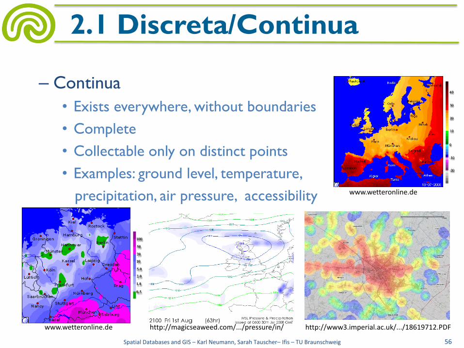
– Continua
• Exists everywhere, without boundaries
• Complete
• Collectable only on distinct points
• Examples: ground level, temperature,
precipitation, air pressure, accessibility
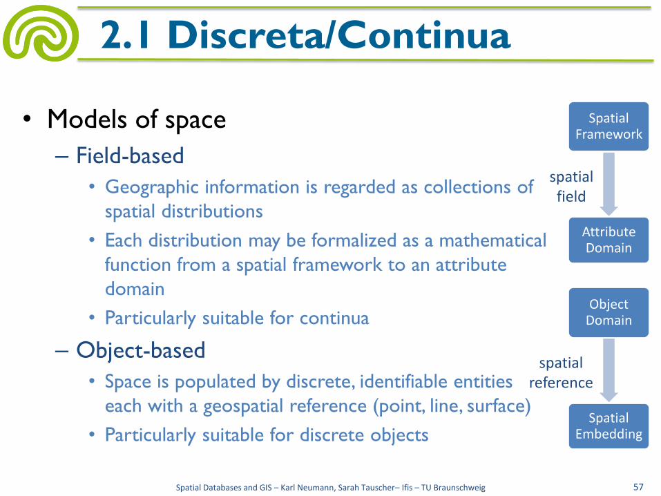
• Models of space
– Field-based
• Geographic information is regarded as collections of
spatial distributions
• Each distribution may be formalized as a mathematical
function from a spatial framework to an attribute
domain
• Particularly suitable for continua
– Object-based
• Space is populated by discrete, identifiable entities
each with a geospatial reference (point, line, surface)
• Particularly suitable for discrete objects
Spatial Databases and GIS – Karl Neumann, Sarah Tauscher– Ifis – TU Braunschweig 57
2.1 Discreta/Continua
Spatial Framework
Attribute Domain
spatial field
Object Domain
Spatial Embedding
spatial reference
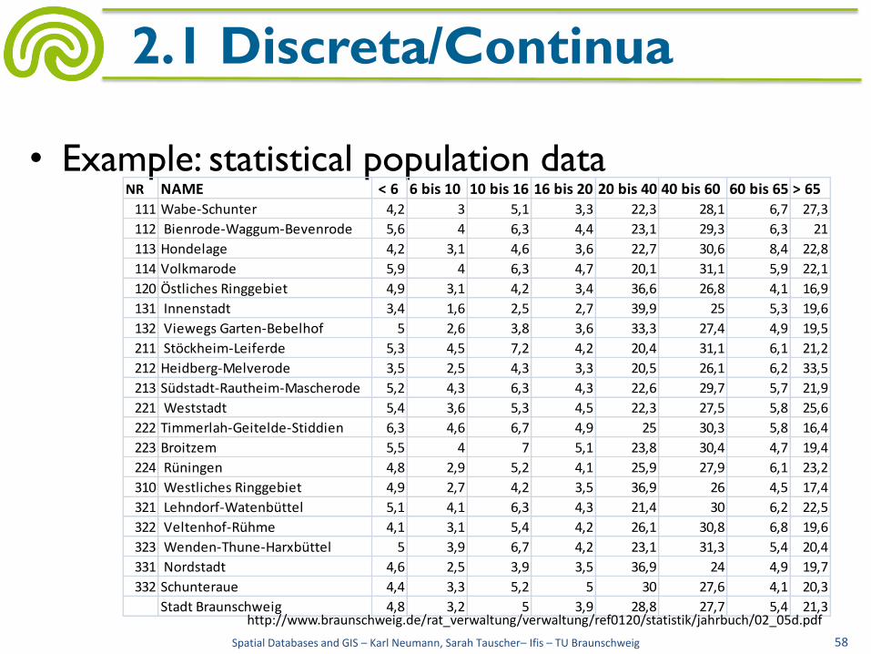
• Example: statistical population data
Spatial Databases and GIS – Karl Neumann, Sarah Tauscher– Ifis – TU Braunschweig 58
2.1 Discreta/Continua
NR NAME < 6 6 bis 10 10 bis 16 16 bis 20 20 bis 40 40 bis 60 60 bis 65 > 65
111 Wabe-Schunter 4,2 3 5,1 3,3 22,3 28,1 6,7 27,3
112 Bienrode-Waggum-Bevenrode 5,6 4 6,3 4,4 23,1 29,3 6,3 21
113 Hondelage 4,2 3,1 4,6 3,6 22,7 30,6 8,4 22,8
114 Volkmarode 5,9 4 6,3 4,7 20,1 31,1 5,9 22,1
120 Östliches Ringgebiet 4,9 3,1 4,2 3,4 36,6 26,8 4,1 16,9
131 Innenstadt 3,4 1,6 2,5 2,7 39,9 25 5,3 19,6
132 Viewegs Garten-Bebelhof 5 2,6 3,8 3,6 33,3 27,4 4,9 19,5
211 Stöckheim-Leiferde 5,3 4,5 7,2 4,2 20,4 31,1 6,1 21,2
212 Heidberg-Melverode 3,5 2,5 4,3 3,3 20,5 26,1 6,2 33,5
213 Südstadt-Rautheim-Mascherode 5,2 4,3 6,3 4,3 22,6 29,7 5,7 21,9
221 Weststadt 5,4 3,6 5,3 4,5 22,3 27,5 5,8 25,6
222 Timmerlah-Geitelde-Stiddien 6,3 4,6 6,7 4,9 25 30,3 5,8 16,4
223 Broitzem 5,5 4 7 5,1 23,8 30,4 4,7 19,4
224 Rüningen 4,8 2,9 5,2 4,1 25,9 27,9 6,1 23,2
310 Westliches Ringgebiet 4,9 2,7 4,2 3,5 36,9 26 4,5 17,4
321 Lehndorf-Watenbüttel 5,1 4,1 6,3 4,3 21,4 30 6,2 22,5
322 Veltenhof-Rühme 4,1 3,1 5,4 4,2 26,1 30,8 6,8 19,6
323 Wenden-Thune-Harxbüttel 5 3,9 6,7 4,2 23,1 31,3 5,4 20,4
331 Nordstadt 4,6 2,5 3,9 3,5 36,9 24 4,9 19,7
332 Schunteraue 4,4 3,3 5,2 5 30 27,6 4,1 20,3
Stadt Braunschweig 4,8 3,2 5 3,9 28,8 27,7 5,4 21,3http://www.braunschweig.de/rat_verwaltung/verwaltung/ref0120/statistik/jahrbuch/02_05d.pdf
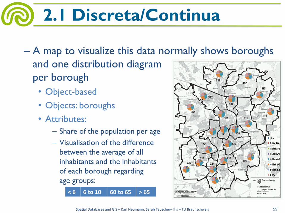
– A map to visualize this data normally shows boroughs
and one distribution diagram
per borough
• Object-based
• Objects: boroughs
• Attributes:
– Share of the population per age
– Visualisation of the difference
between the average of all
inhabitants and the inhabitants
of each borough regarding
age groups:
Spatial Databases and GIS – Karl Neumann, Sarah Tauscher– Ifis – TU Braunschweig 59
2.1 Discreta/Continua
< 6 6 to 10 60 to 65 > 65
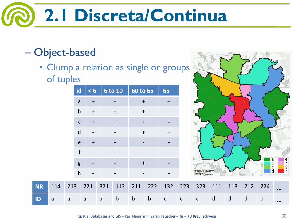
– Object-based
• Clump a relation as single or groups
of tuples
Spatial Databases and GIS – Karl Neumann, Sarah Tauscher– Ifis – TU Braunschweig 60
2.1 Discreta/Continua
id < 6 6 to 10 60 to 65 65
a + + + +
b + + + -
c + + - -
d - - + +
e + - - -
f - + - -
g - - + -
h - - - -
NR 114 213 221 321 112 211 222 132 223 323 111 113 212 224 …
ID a a a a b b b c c c d d d d …
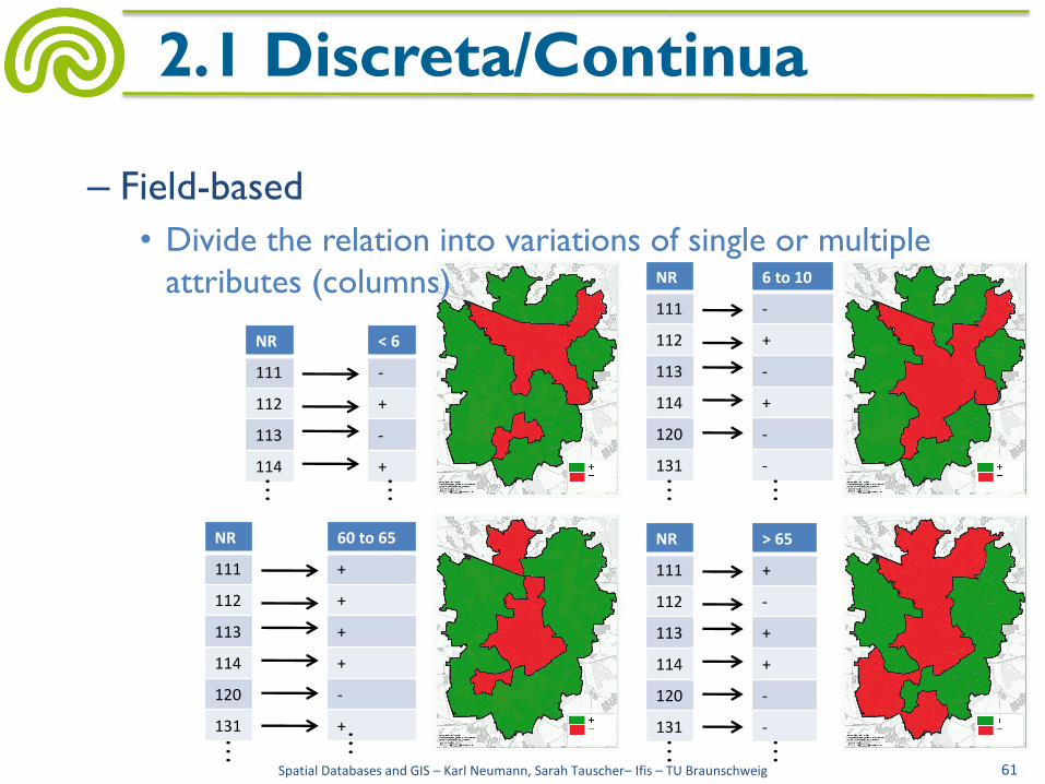
– Field-based
• Divide the relation into variations of single or multiple
attributes (columns)
Spatial Databases and GIS – Karl Neumann, Sarah Tauscher– Ifis – TU Braunschweig 61
2.1 Discreta/Continua
NR
111
112
113
114
< 6
-
+
-
+
NR
111
112
113
114
120
131
6 to 10
-
+
-
+
-
-
NR
111
112
113
114
120
131
60 to 65
+
+
+
+
-
+
NR
111
112
113
114
120
131
> 65
+
-
+
+
-
-
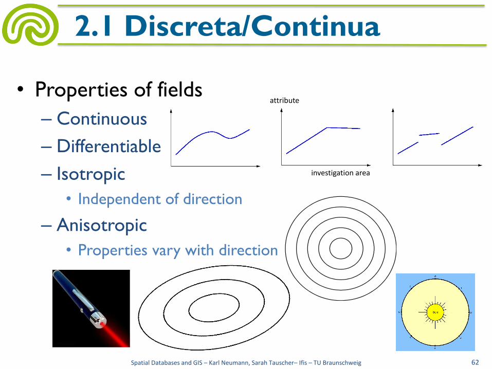
• Properties of fields
– Continuous
– Differentiable
– Isotropic
• Independent of direction
– Anisotropic
• Properties vary with direction
Spatial Databases and GIS – Karl Neumann, Sarah Tauscher– Ifis – TU Braunschweig 62
2.1 Discreta/Continua
attribute
investigation area
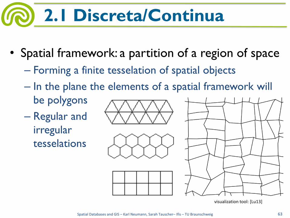
• Spatial framework: a partition of a region of space
– Forming a finite tesselation of spatial objects
– In the plane the elements of a spatial framework will
be polygons
– Regular and
irregular
tesselations
Spatial Databases and GIS – Karl Neumann, Sarah Tauscher– Ifis – TU Braunschweig 63
2.1 Discreta/Continua
visualization tool: [Lu13]
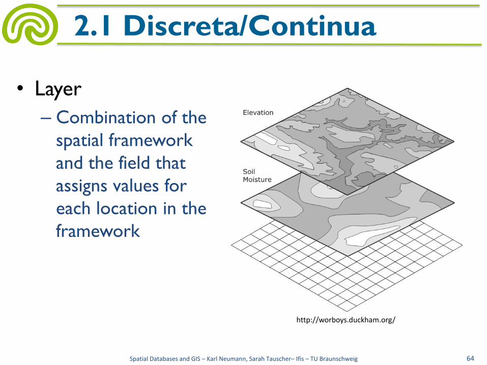
• Layer
– Combination of the
spatial framework
and the field that
assigns values for
each location in the
framework
Spatial Databases and GIS – Karl Neumann, Sarah Tauscher– Ifis – TU Braunschweig 64
2.1 Discreta/Continua
http://worboys.duckham.org/
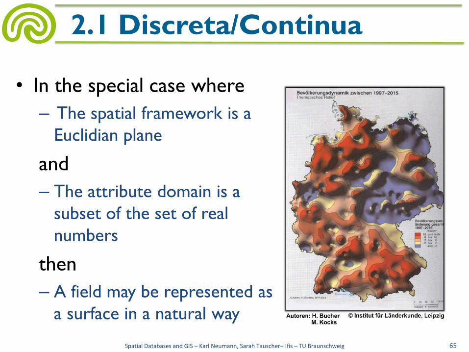
• In the special case where
– The spatial framework is a
Euclidian plane
and
– The attribute domain is a
subset of the set of real
numbers
then
– A field may be represented as
a surface in a natural way
Spatial Databases and GIS – Karl Neumann, Sarah Tauscher– Ifis – TU Braunschweig 65
2.1 Discreta/Continua
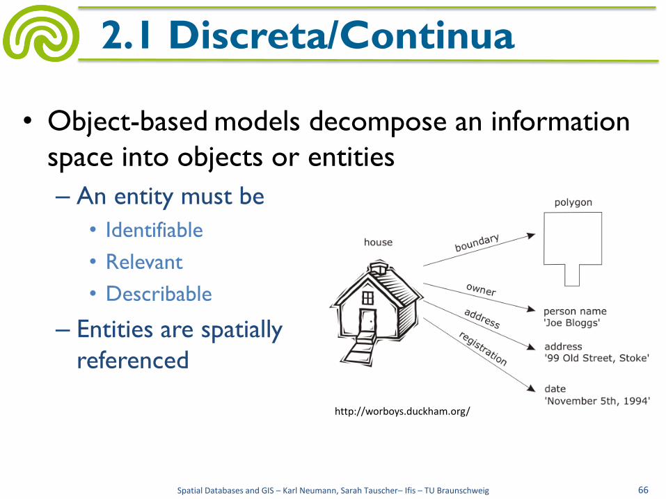
• Object-based models decompose an information
space into objects or entities
– An entity must be
• Identifiable
• Relevant
• Describable
– Entities are spatially
referenced
Spatial Databases and GIS – Karl Neumann, Sarah Tauscher– Ifis – TU Braunschweig 66
2.1 Discreta/Continua
http://worboys.duckham.org/
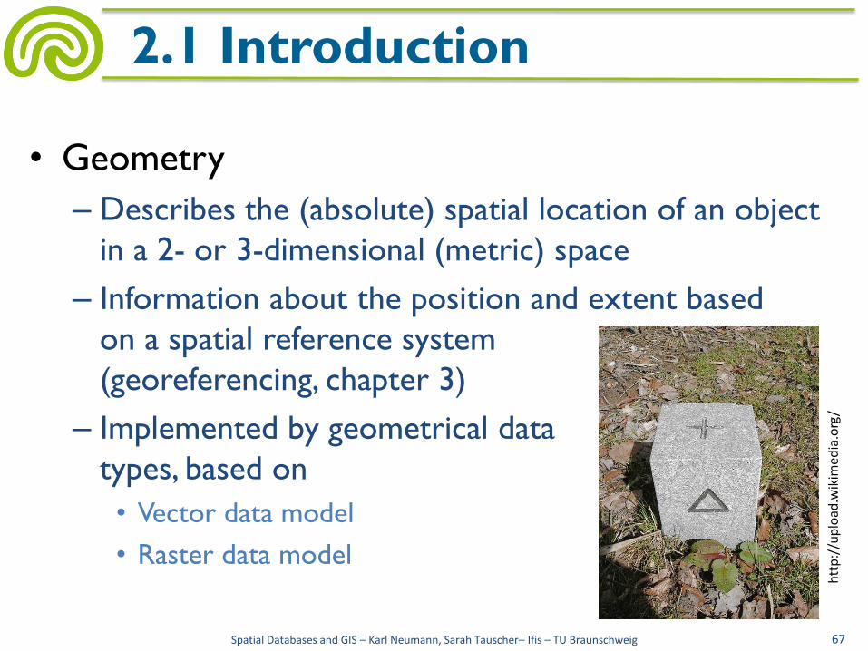
• Geometry
– Describes the (absolute) spatial location of an object
in a 2- or 3-dimensional (metric) space
– Information about the position and extent based
on a spatial reference system
(georeferencing, chapter 3)
– Implemented by geometrical data
types, based on
• Vector data model
• Raster data model
Spatial Databases and GIS – Karl Neumann, Sarah Tauscher– Ifis – TU Braunschweig 67
2.1 Introduction
htt
p:/
/up
load
.wik
imed
ia.o
rg/
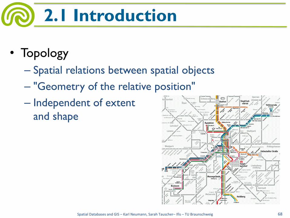
• Topology
– Spatial relations between spatial objects
– "Geometry of the relative position"
– Independent of extent
and shape
Spatial Databases and GIS – Karl Neumann, Sarah Tauscher– Ifis – TU Braunschweig 68
2.1 Introduction
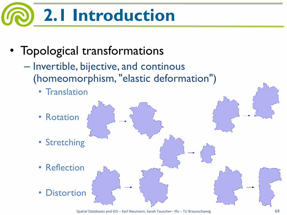
• Topological transformations
– Invertible, bijective, and continous (homeomorphism, "elastic deformation")
• Translation
• Rotation
• Stretching
• Reflection
• Distortion
Spatial Databases and GIS – Karl Neumann, Sarah Tauscher– Ifis – TU Braunschweig 69
2.1 Introduction
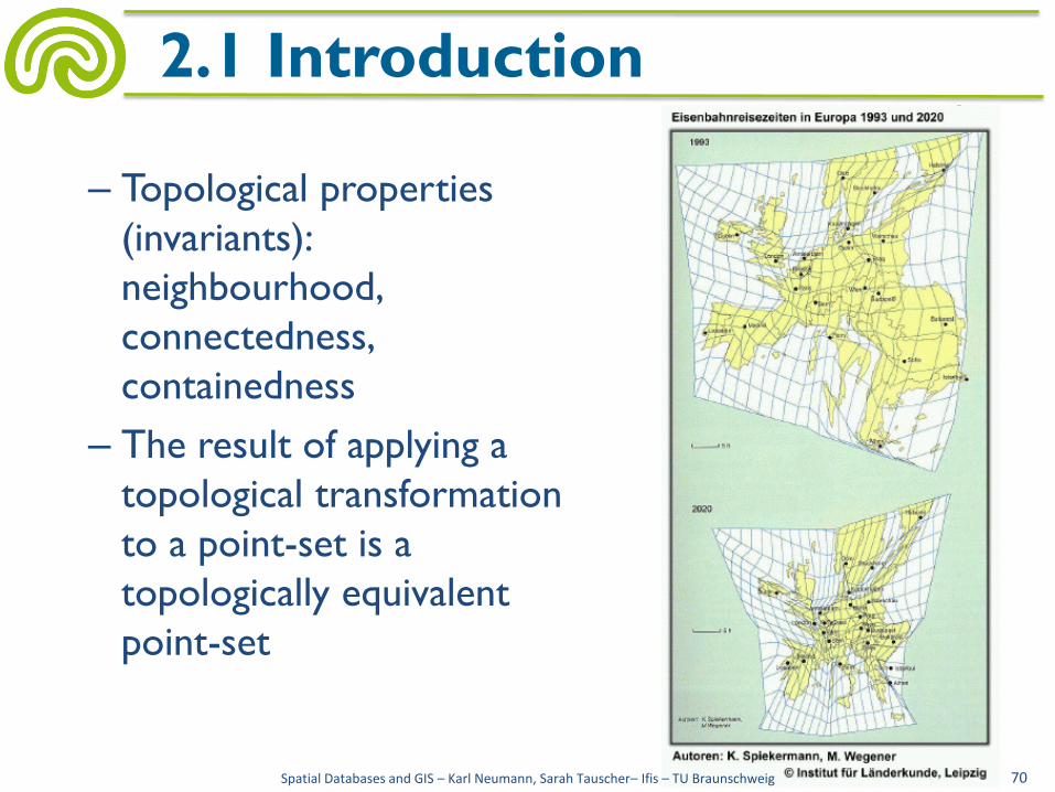
– Topological properties
(invariants):
neighbourhood,
connectedness,
containedness
– The result of applying a
topological transformation
to a point-set is a
topologically equivalent
point-set
Spatial Databases and GIS – Karl Neumann, Sarah Tauscher– Ifis – TU Braunschweig 70
2.1 Introduction
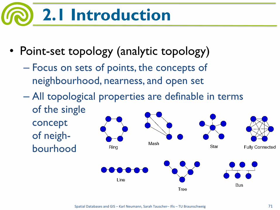
• Point-set topology (analytic topology)
– Focus on sets of points, the concepts of
neighbourhood, nearness, and open set
– All topological properties are definable in terms
of the single
concept
of neigh-
bourhood
Spatial Databases and GIS – Karl Neumann, Sarah Tauscher– Ifis – TU Braunschweig 71
2.1 Introduction
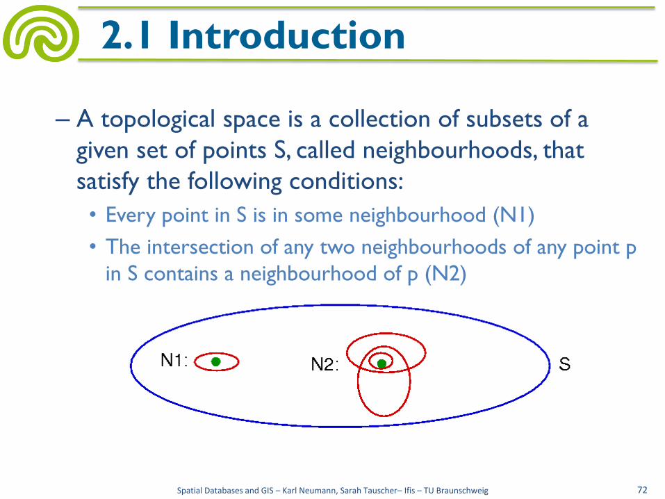
– A topological space is a collection of subsets of a
given set of points S, called neighbourhoods, that
satisfy the following conditions:
• Every point in S is in some neighbourhood (N1)
• The intersection of any two neighbourhoods of any point p
in S contains a neighbourhood of p (N2)
Spatial Databases and GIS – Karl Neumann, Sarah Tauscher– Ifis – TU Braunschweig 72
2.1 Introduction
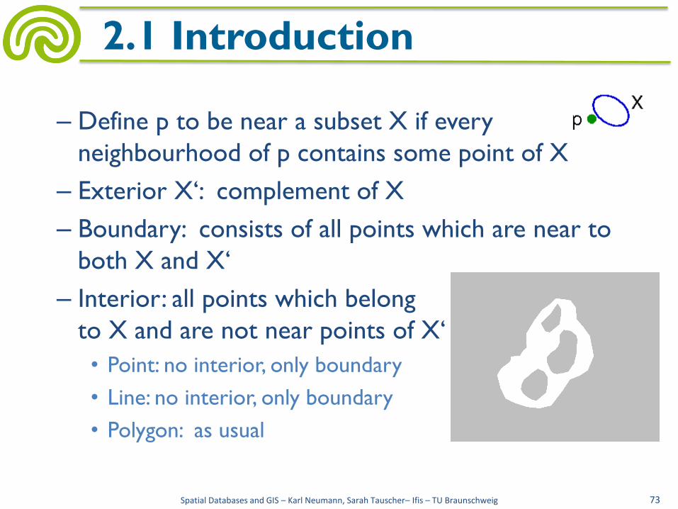
– Define p to be near a subset X if every
neighbourhood of p contains some point of X
– Exterior X‘: complement of X
– Boundary: consists of all points which are near to
both X and X‘
– Interior: all points which belong
to X and are not near points of X‘
• Point: no interior, only boundary
• Line: no interior, only boundary
• Polygon: as usual
Spatial Databases and GIS – Karl Neumann, Sarah Tauscher– Ifis – TU Braunschweig 73
2.1 Introduction
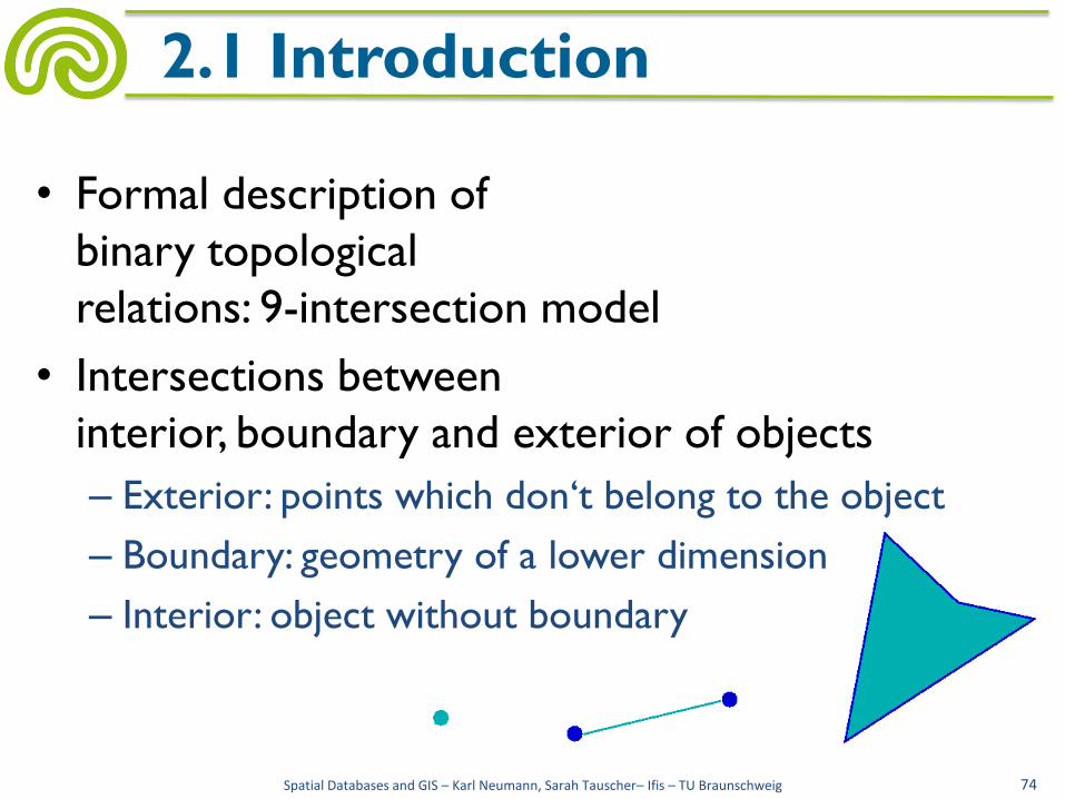
• Formal description of
binary topological
relations: 9-intersection model
• Intersections between
interior, boundary and exterior of objects
– Exterior: points which don‘t belong to the object
– Boundary: geometry of a lower dimension
– Interior: object without boundary
Spatial Databases and GIS – Karl Neumann, Sarah Tauscher– Ifis – TU Braunschweig 74
2.1 Introduction
EQUAL DISJOINT MEET
OVERLAP COVERS COVEREDBY
INSIDE CONTAINS
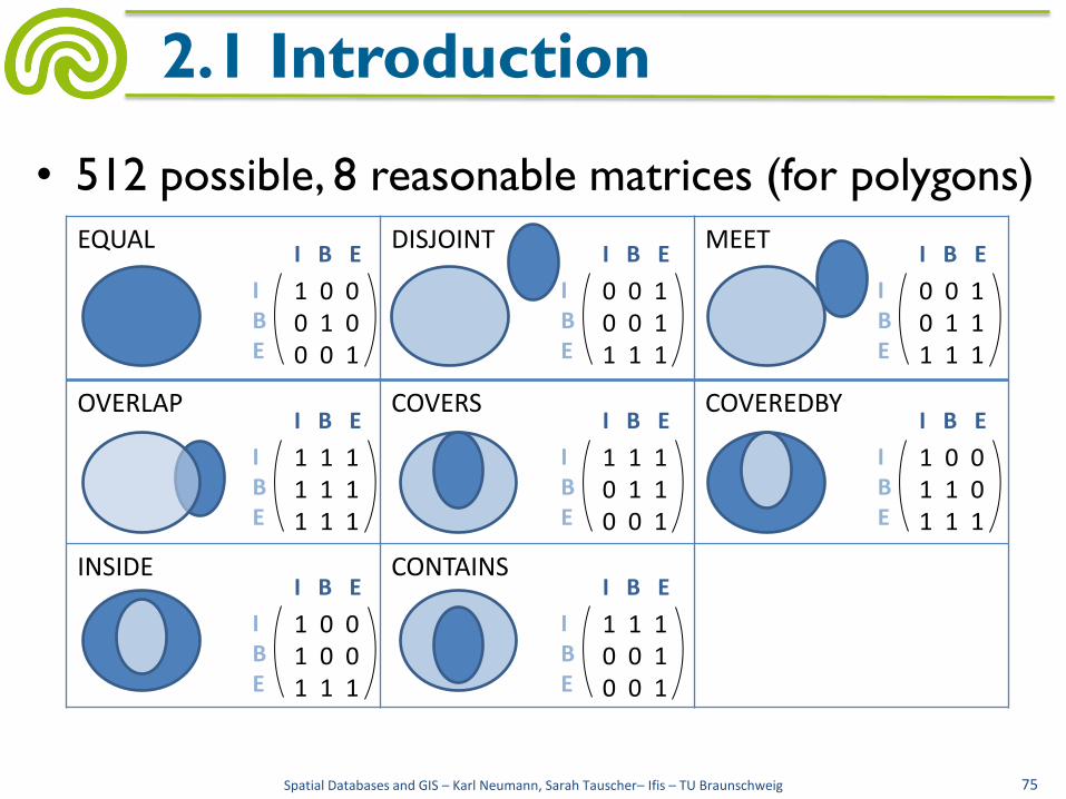
• 512 possible, 8 reasonable matrices (for polygons)
Spatial Databases and GIS – Karl Neumann, Sarah Tauscher– Ifis – TU Braunschweig 75
2.1 Introduction
I B E
I B E
1 0 0 0 1 0 0 0 1
I B E
I B E
0 0 1 0 0 1 1 1 1
I B E
I B E
0 0 1 0 1 1 1 1 1
I B E
I B E
1 1 1 1 1 1 1 1 1
I B E
I B E
1 1 1 0 1 1 0 0 1
I B E
I B E
1 0 0 1 1 0 1 1 1
I B E
I B E
1 0 0 1 0 0 1 1 1
I B E
I B E
1 1 1 0 0 1 0 0 1
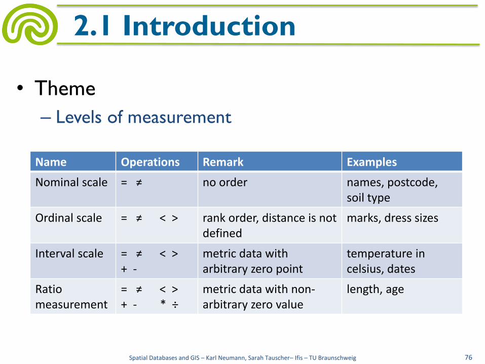
• Theme
– Levels of measurement
Spatial Databases and GIS – Karl Neumann, Sarah Tauscher– Ifis – TU Braunschweig 76
2.1 Introduction
Name Operations Remark Examples
Nominal scale = ≠ no order names, postcode, soil type
Ordinal scale = ≠ < > rank order, distance is not defined
marks, dress sizes
Interval scale = ≠ < > + -
metric data with arbitrary zero point
temperature in celsius, dates
Ratio measurement
= ≠ < > + - * ÷
metric data with non-arbitrary zero value
length, age
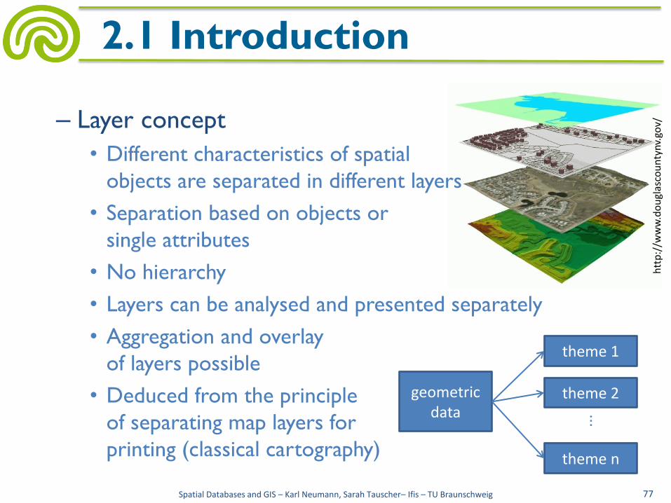
– Layer concept
• Different characteristics of spatial
objects are separated in different layers
• Separation based on objects or
single attributes
• No hierarchy
• Layers can be analysed and presented separately
• Aggregation and overlay
of layers possible
• Deduced from the principle
of separating map layers for
printing (classical cartography)
Spatial Databases and GIS – Karl Neumann, Sarah Tauscher– Ifis – TU Braunschweig 77
2.1 Introduction
geometric data
theme 1
theme 2
theme n
...
htt
p:/
/ww
w.d
ou
glas
cou
nty
nv.g
ov/
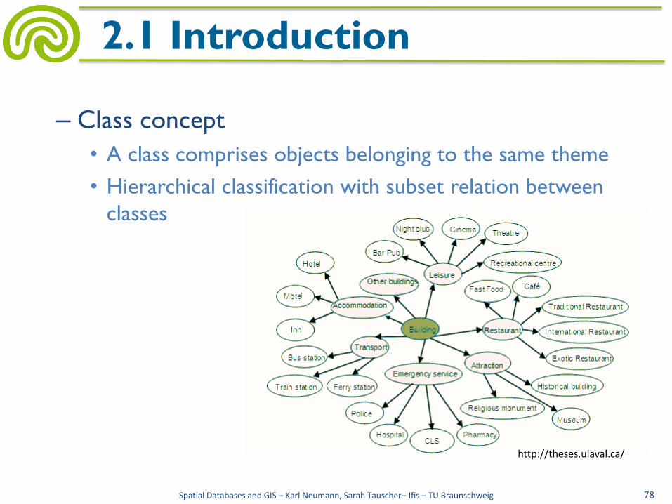
– Class concept
• A class comprises objects belonging to the same theme
• Hierarchical classification with subset relation between
classes
Spatial Databases and GIS – Karl Neumann, Sarah Tauscher– Ifis – TU Braunschweig 78
2.1 Introduction
http://theses.ulaval.ca/
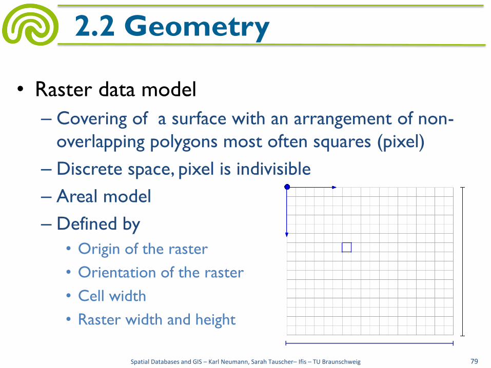
• Raster data model
– Covering of a surface with an arrangement of non-
overlapping polygons most often squares (pixel)
– Discrete space, pixel is indivisible
– Areal model
– Defined by
• Origin of the raster
• Orientation of the raster
• Cell width
• Raster width and height
Spatial Databases and GIS – Karl Neumann, Sarah Tauscher– Ifis – TU Braunschweig 79
2.2 Geometry
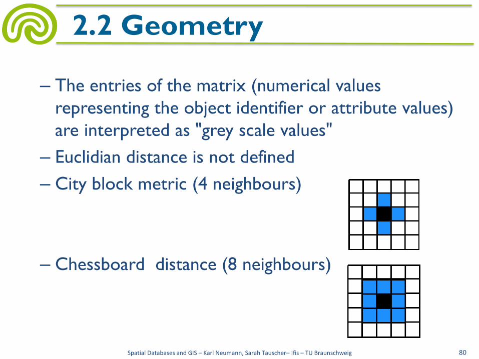
– The entries of the matrix (numerical values
representing the object identifier or attribute values)
are interpreted as "grey scale values"
– Euclidian distance is not defined
– City block metric (4 neighbours)
– Chessboard distance (8 neighbours)
Spatial Databases and GIS – Karl Neumann, Sarah Tauscher– Ifis – TU Braunschweig 80
2.2 Geometry
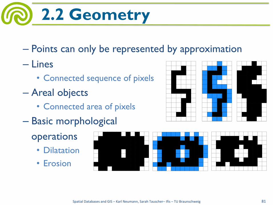
– Points can only be represented by approximation
– Lines
• Connected sequence of pixels
– Areal objects
• Connected area of pixels
– Basic morphological
operations
• Dilatation
• Erosion
Spatial Databases and GIS – Karl Neumann, Sarah Tauscher– Ifis – TU Braunschweig 81
2.2 Geometry
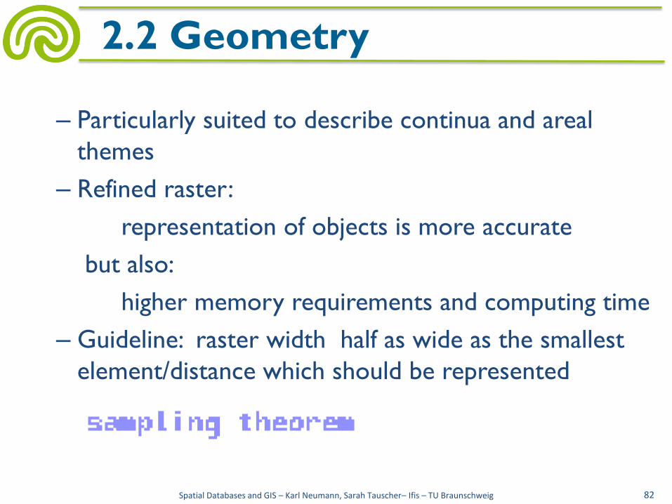
– Particularly suited to describe continua and areal
themes
– Refined raster:
representation of objects is more accurate
but also:
higher memory requirements and computing time
– Guideline: raster width half as wide as the smallest
element/distance which should be represented
Spatial Databases and GIS – Karl Neumann, Sarah Tauscher– Ifis – TU Braunschweig 82
2.2 Geometry
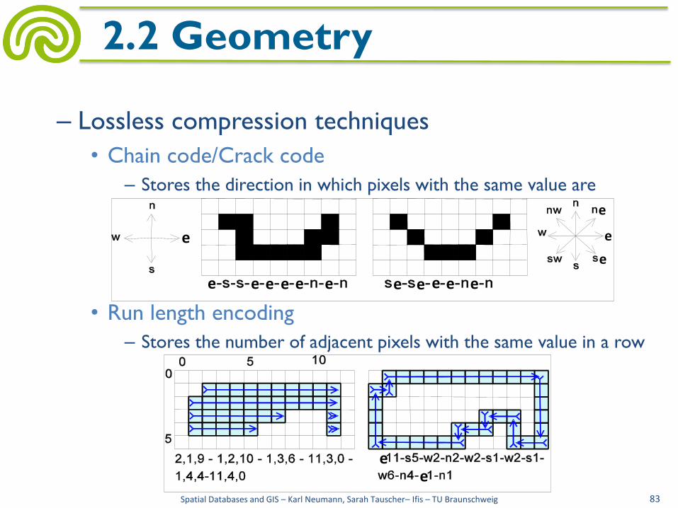
– Lossless compression techniques
• Chain code/Crack code
– Stores the direction in which pixels with the same value are
• Run length encoding
– Stores the number of adjacent pixels with the same value in a row
Spatial Databases and GIS – Karl Neumann, Sarah Tauscher– Ifis – TU Braunschweig 83
2.2 Geometry
e e
e e e e e e e e e e e
e
e
e e
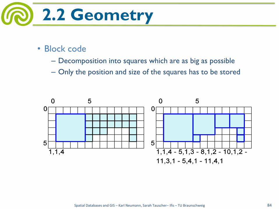
• Block code
– Decomposition into squares which are as big as possible
– Only the position and size of the squares has to be stored
Spatial Databases and GIS – Karl Neumann, Sarah Tauscher– Ifis – TU Braunschweig 84
2.2 Geometry
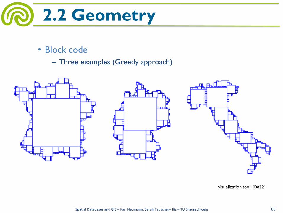
• Block code
– Three examples (Greedy approach)
Spatial Databases and GIS – Karl Neumann, Sarah Tauscher– Ifis – TU Braunschweig 85
2.2 Geometry
visualization tool: [Da12]
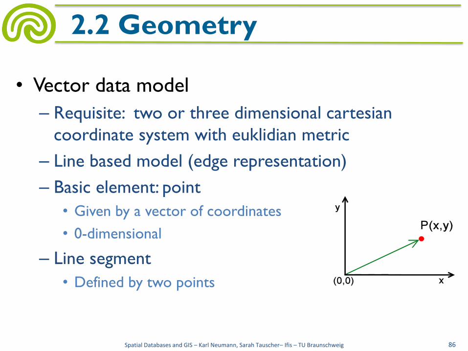
• Vector data model
– Requisite: two or three dimensional cartesian
coordinate system with euklidian metric
– Line based model (edge representation)
– Basic element: point
• Given by a vector of coordinates
• 0-dimensional
– Line segment
• Defined by two points
Spatial Databases and GIS – Karl Neumann, Sarah Tauscher– Ifis – TU Braunschweig 86
2.2 Geometry
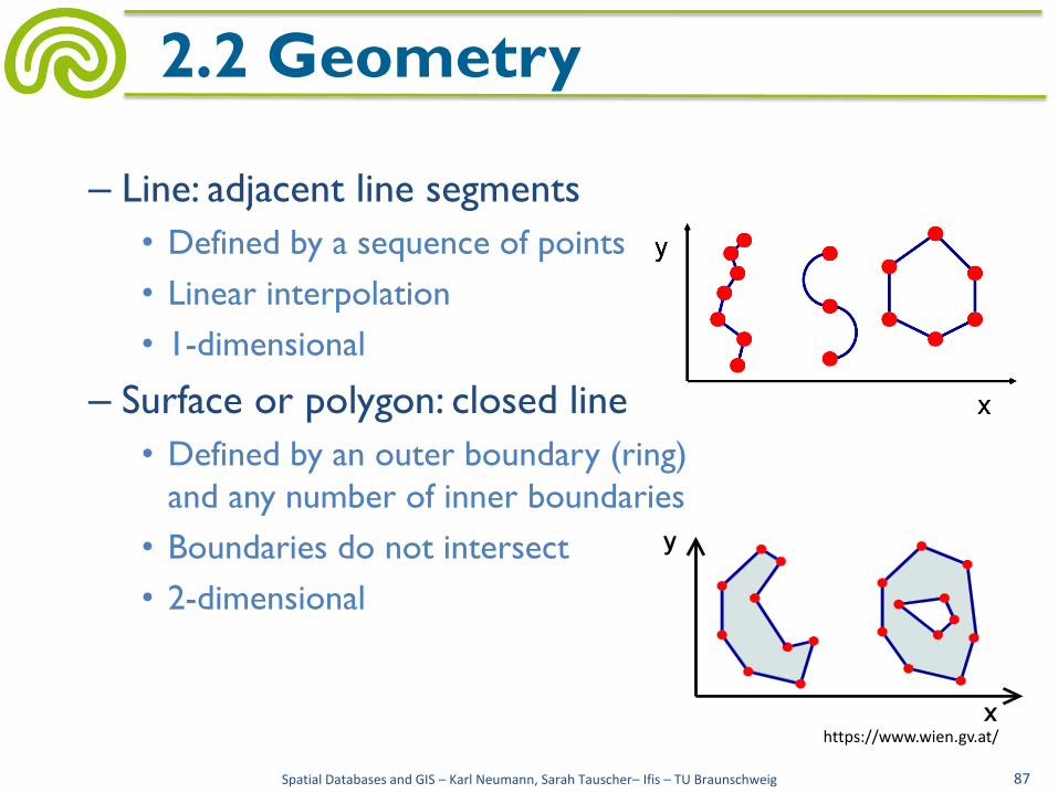
– Line: adjacent line segments
• Defined by a sequence of points
• Linear interpolation
• 1-dimensional
– Surface or polygon: closed line
• Defined by an outer boundary (ring)
and any number of inner boundaries
• Boundaries do not intersect
• 2-dimensional
Spatial Databases and GIS – Karl Neumann, Sarah Tauscher– Ifis – TU Braunschweig 87
2.2 Geometry
https://www.wien.gv.at/
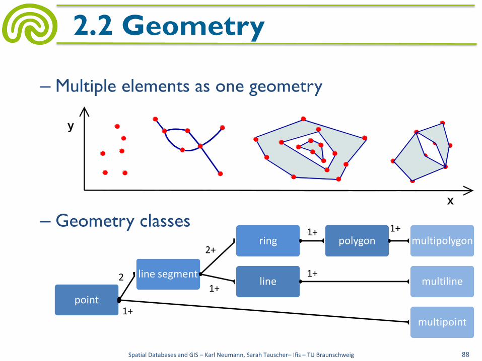
– Multiple elements as one geometry
– Geometry classes
Spatial Databases and GIS – Karl Neumann, Sarah Tauscher– Ifis – TU Braunschweig 88
2.2 Geometry
point
line segment
ring polygon multipolygon
line multiline
multipoint
2+
2
1+
1+
1+
1+
1+
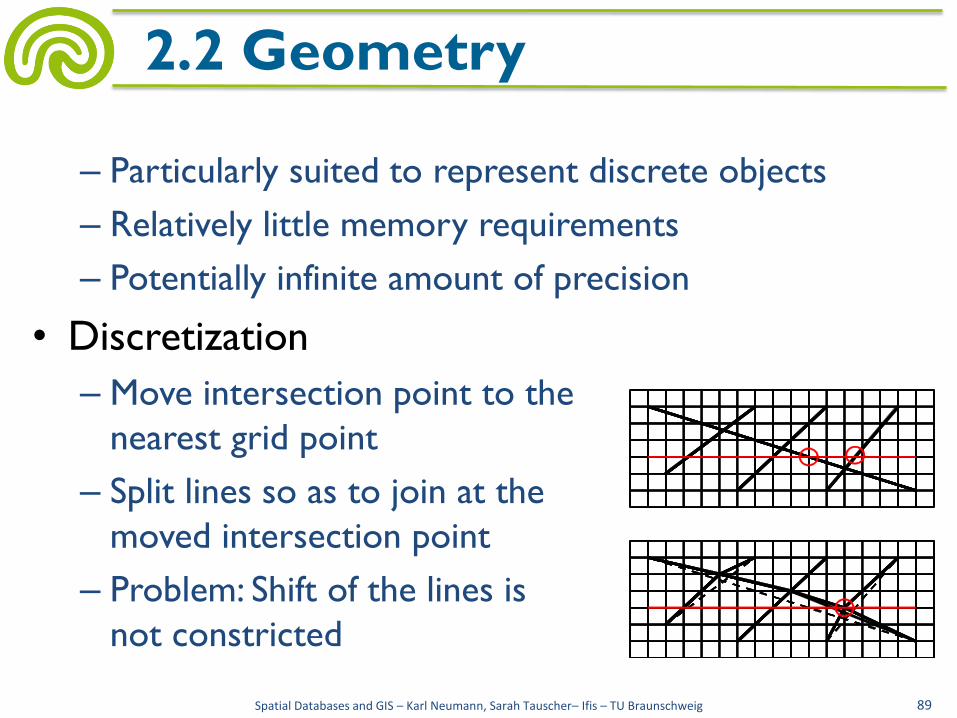
– Particularly suited to represent discrete objects
– Relatively little memory requirements
– Potentially infinite amount of precision
• Discretization
– Move intersection point to the
nearest grid point
– Split lines so as to join at the
moved intersection point
– Problem: Shift of the lines is
not constricted
Spatial Databases and GIS – Karl Neumann, Sarah Tauscher– Ifis – TU Braunschweig 89
2.2 Geometry
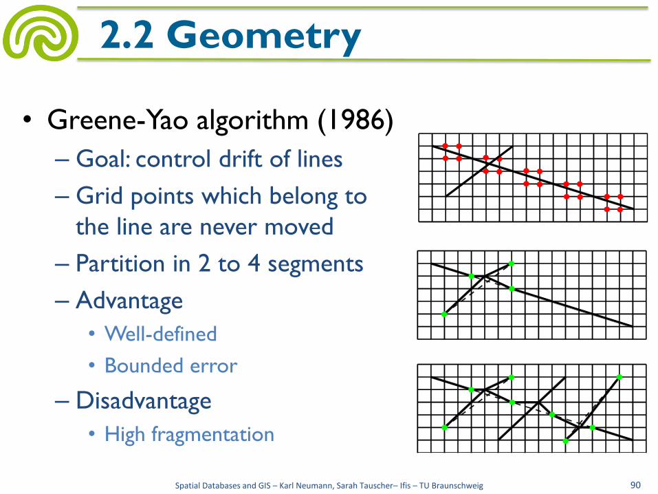
• Greene-Yao algorithm (1986)
– Goal: control drift of lines
– Grid points which belong to
the line are never moved
– Partition in 2 to 4 segments
– Advantage
• Well-defined
• Bounded error
– Disadvantage
• High fragmentation
Spatial Databases and GIS – Karl Neumann, Sarah Tauscher– Ifis – TU Braunschweig 90
2.2 Geometry
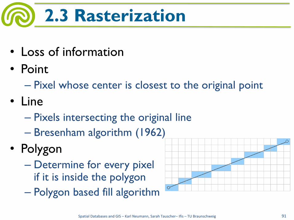
• Loss of information
• Point
– Pixel whose center is closest to the original point
• Line
– Pixels intersecting the original line
– Bresenham algorithm (1962)
• Polygon
– Determine for every pixel if it is inside the polygon
– Polygon based fill algorithm
Spatial Databases and GIS – Karl Neumann, Sarah Tauscher– Ifis – TU Braunschweig 91
2.3 Rasterization
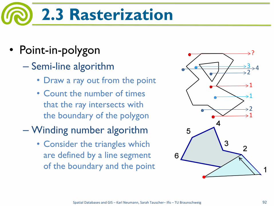
• Point-in-polygon
– Semi-line algorithm
• Draw a ray out from the point
• Count the number of times
that the ray intersects with
the boundary of the polygon
– Winding number algorithm
• Consider the triangles which
are defined by a line segment
of the boundary and the point
Spatial Databases and GIS – Karl Neumann, Sarah Tauscher– Ifis – TU Braunschweig 92
2.3 Rasterization
1
3
2
2 4
1
1
?
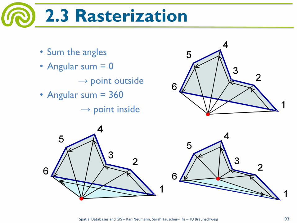
• Sum the angles
• Angular sum = 0
→ point outside
• Angular sum = 360
→ point inside
Spatial Databases and GIS – Karl Neumann, Sarah Tauscher– Ifis – TU Braunschweig 93
2.3 Rasterization
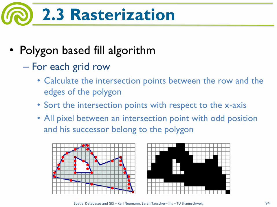
• Polygon based fill algorithm
– For each grid row
• Calculate the intersection points between the row and the
edges of the polygon
• Sort the intersection points with respect to the x-axis
• All pixel between an intersection point with odd position
and his successor belong to the polygon
Spatial Databases and GIS – Karl Neumann, Sarah Tauscher– Ifis – TU Braunschweig 94
2.3 Rasterization
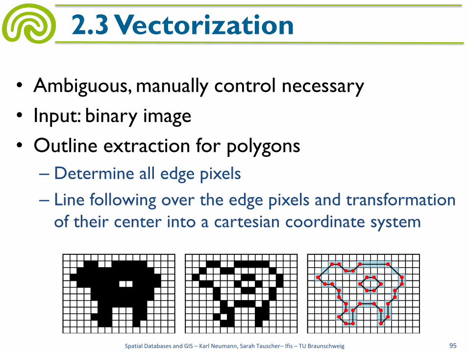
• Ambiguous, manually control necessary
• Input: binary image
• Outline extraction for polygons
– Determine all edge pixels
– Line following over the edge pixels and transformation
of their center into a cartesian coordinate system
Spatial Databases and GIS – Karl Neumann, Sarah Tauscher– Ifis – TU Braunschweig 95
2.3 Vectorization
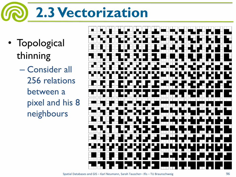
• Topological
thinning
– Consider all
256 relations
between a
pixel and his 8
neighbours
Spatial Databases and GIS – Karl Neumann, Sarah Tauscher– Ifis – TU Braunschweig 96
2.3 Vectorization
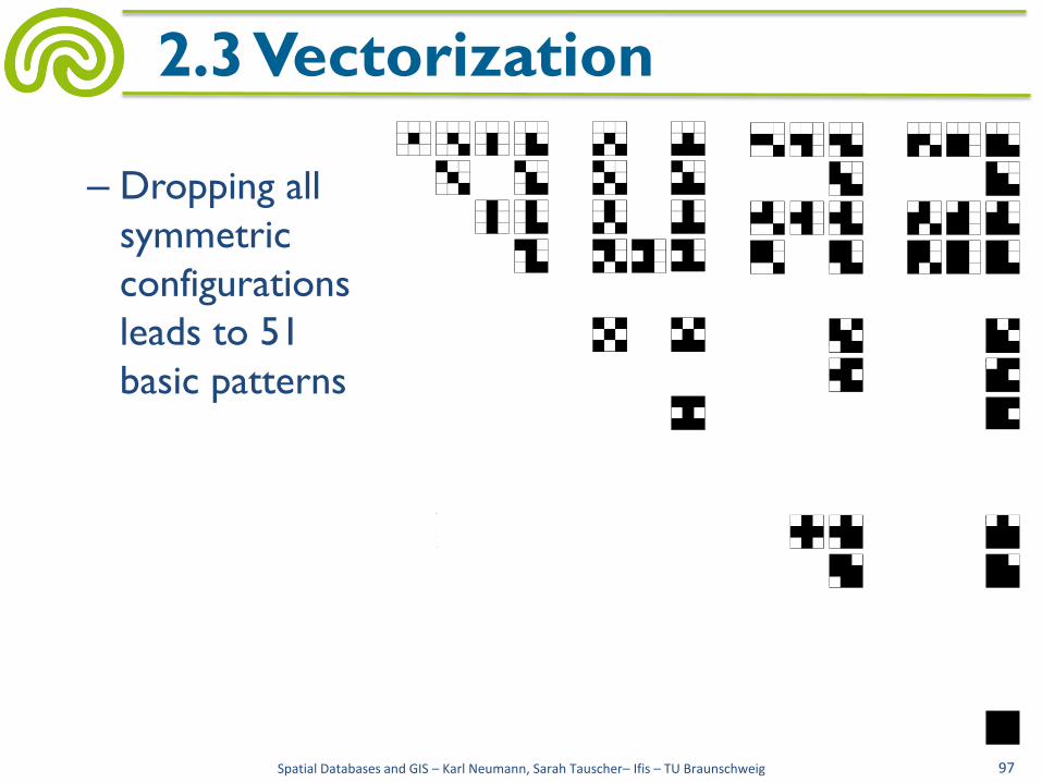
– Dropping all
symmetric
configurations
leads to 51
basic patterns
Spatial Databases and GIS – Karl Neumann, Sarah Tauscher– Ifis – TU Braunschweig 97
2.3 Vectorization
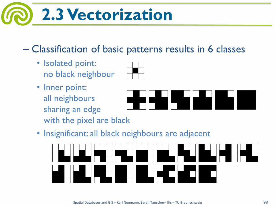
– Classification of basic patterns results in 6 classes
• Isolated point:
no black neighbour
• Inner point:
all neighbours
sharing an edge
with the pixel are black
• Insignificant: all black neighbours are adjacent
Spatial Databases and GIS – Karl Neumann, Sarah Tauscher– Ifis – TU Braunschweig 98
2.3 Vectorization
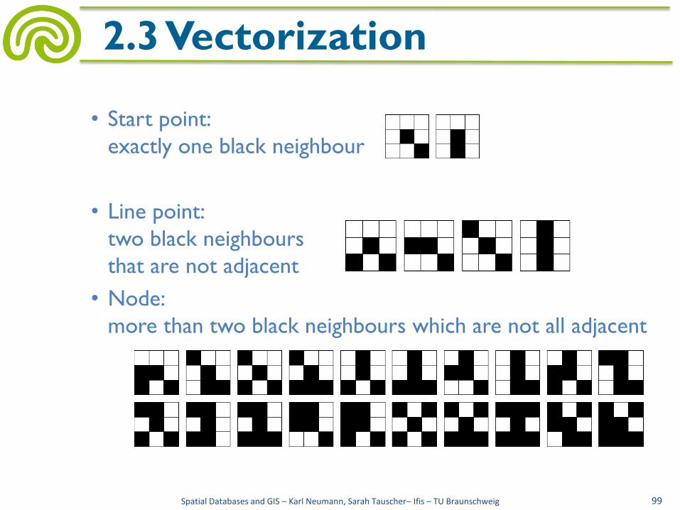
• Start point:
exactly one black neighbour
• Line point:
two black neighbours
that are not adjacent
• Node:
more than two black neighbours which are not all adjacent
Spatial Databases and GIS – Karl Neumann, Sarah Tauscher– Ifis – TU Braunschweig 99
2.3 Vectorization
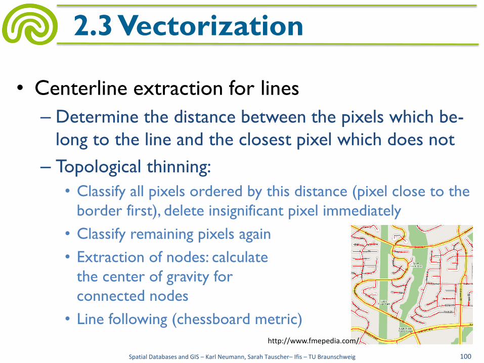
• Centerline extraction for lines
– Determine the distance between the pixels which be-
long to the line and the closest pixel which does not
– Topological thinning:
• Classify all pixels ordered by this distance (pixel close to the
border first), delete insignificant pixel immediately
• Classify remaining pixels again
• Extraction of nodes: calculate
the center of gravity for
connected nodes
• Line following (chessboard metric)
Spatial Databases and GIS – Karl Neumann, Sarah Tauscher– Ifis – TU Braunschweig 100
2.3 Vectorization
http://www.fmepedia.com/
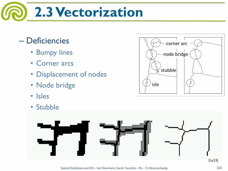
– Deficiencies
• Bumpy lines
• Corner arcs
• Displacement of nodes
• Node bridge
• Isles
• Stubble
Spatial Databases and GIS – Karl Neumann, Sarah Tauscher– Ifis – TU Braunschweig 101
2.3 Vectorization
[La13]
corner arc
node bridge
stubble
isle
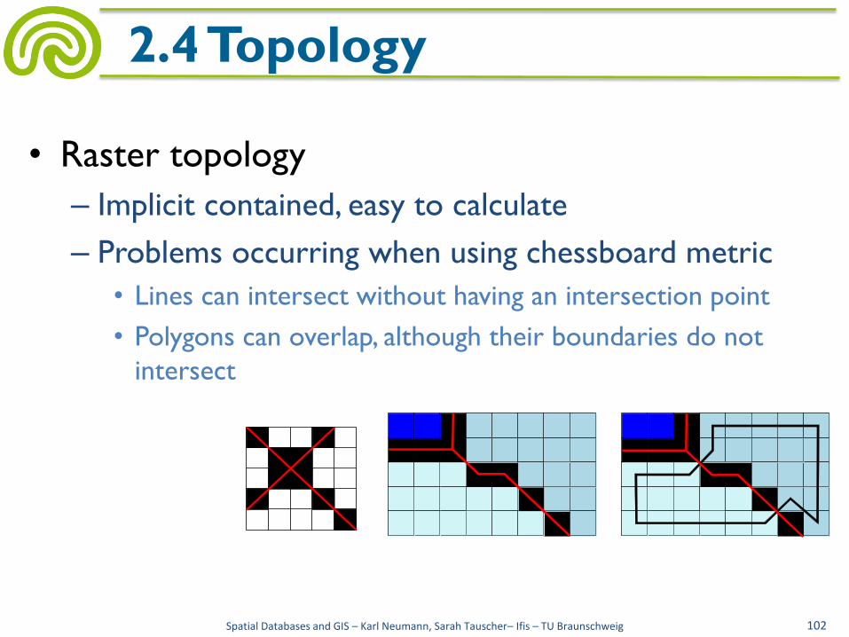
• Raster topology
– Implicit contained, easy to calculate
– Problems occurring when using chessboard metric
• Lines can intersect without having an intersection point
• Polygons can overlap, although their boundaries do not
intersect
Spatial Databases and GIS – Karl Neumann, Sarah Tauscher– Ifis – TU Braunschweig 102
2.4 Topology
• Metric space implies topological space, i.e. it is
possible to determine the topological relations
between objects if their geometries are known
• Access and computations are normally more
efficient if the topology is given explicitly
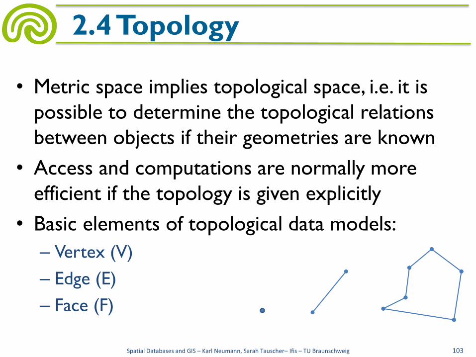
• Basic elements of topological data models:
– Vertex (V)
– Edge (E)
– Face (F)
Spatial Databases and GIS – Karl Neumann, Sarah Tauscher– Ifis – TU Braunschweig 103
2.4 Topology
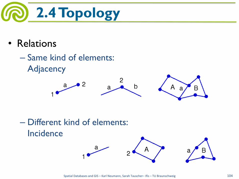
• Relations
– Same kind of elements:
Adjacency
– Different kind of elements:
Incidence
Spatial Databases and GIS – Karl Neumann, Sarah Tauscher– Ifis – TU Braunschweig 104
2.4 Topology
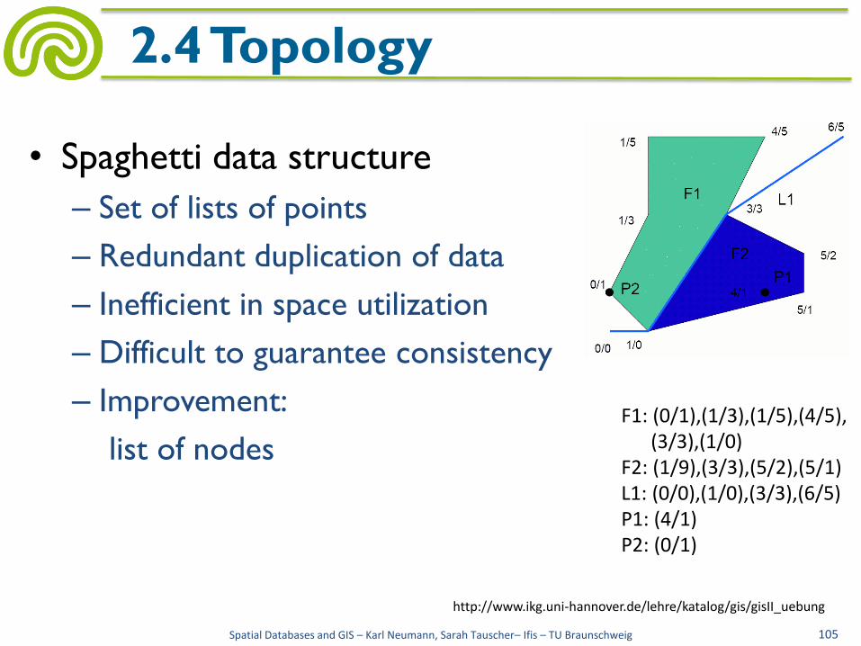
• Spaghetti data structure
– Set of lists of points
– Redundant duplication of data
– Inefficient in space utilization
– Difficult to guarantee consistency
– Improvement:
list of nodes
Spatial Databases and GIS – Karl Neumann, Sarah Tauscher– Ifis – TU Braunschweig 105
2.4 Topology
http://www.ikg.uni-hannover.de/lehre/katalog/gis/gisII_uebung
F1: (0/1),(1/3),(1/5),(4/5), (3/3),(1/0) F2: (1/9),(3/3),(5/2),(5/1) L1: (0/0),(1/0),(3/3),(6/5) P1: (4/1) P2: (0/1)
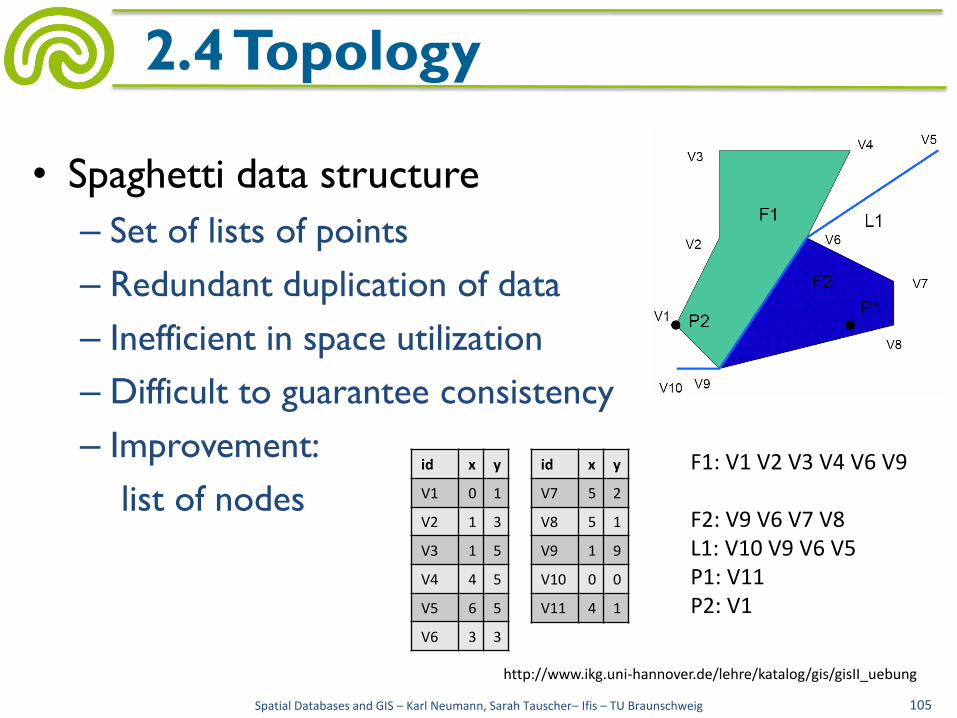
• Spaghetti data structure
– Set of lists of points
– Redundant duplication of data
– Inefficient in space utilization
– Difficult to guarantee consistency
– Improvement:
list of nodes
Spatial Databases and GIS – Karl Neumann, Sarah Tauscher– Ifis – TU Braunschweig 105
2.4 Topology
http://www.ikg.uni-hannover.de/lehre/katalog/gis/gisII_uebung
F1: V1 V2 V3 V4 V6 V9 F2: V9 V6 V7 V8 L1: V10 V9 V6 V5 P1: V11 P2: V1
id x y
V7 5 2
V8 5 1
V9 1 9
V10 0 0
V11 4 1
id x y
V1 0 1
V2 1 3
V3 1 5
V4 4 5
V5 6 5
V6 3 3
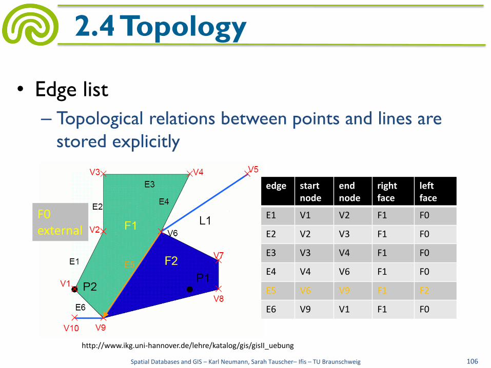
• Edge list
– Topological relations between points and lines are
stored explicitly
Spatial Databases and GIS – Karl Neumann, Sarah Tauscher– Ifis – TU Braunschweig 106
2.4 Topology
http://www.ikg.uni-hannover.de/lehre/katalog/gis/gisII_uebung
edge start node
end node
right face
left face
E1 V1 V2 F1 F0
E2 V2 V3 F1 F0
E3 V3 V4 F1 F0
E4 V4 V6 F1 F0
E5 V6 V9 F1 F2
E6 V9 V1 F1 F0
F0 external
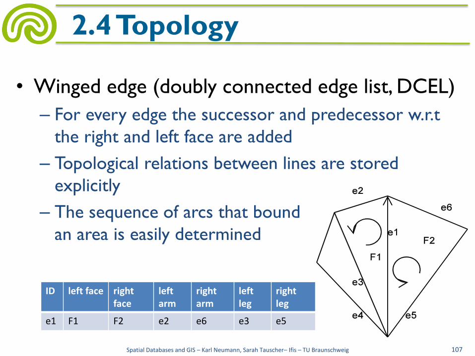
• Winged edge (doubly connected edge list, DCEL)
– For every edge the successor and predecessor w.r.t
the right and left face are added
– Topological relations between lines are stored
explicitly
– The sequence of arcs that bound
an area is easily determined
Spatial Databases and GIS – Karl Neumann, Sarah Tauscher– Ifis – TU Braunschweig 107
2.4 Topology
ID left face right face
left arm
right arm
left leg
right leg
e1 F1 F2 e2 e6 e3 e5
• Integrity constraints for "maps" (US Bureau of
Census)
– Every edge has two incident vertices
– Every edge has two incident faces
– Every face is alternately surrounded by edges and
vertices
– Every vertex is alternately
surrounded by edges and faces
– Edges do not intersect
• Euler characteristic: |V|- |E| + |F| = 2
Spatial Databases and GIS – Karl Neumann, Sarah Tauscher– Ifis – TU Braunschweig 108
2.4 Topology
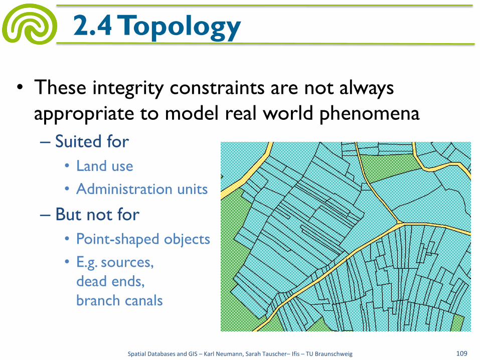
• These integrity constraints are not always
appropriate to model real world phenomena
– Suited for
• Land use
• Administration units
– But not for
• Point-shaped objects
• E.g. sources,
dead ends,
branch canals
Spatial Databases and GIS – Karl Neumann, Sarah Tauscher– Ifis – TU Braunschweig 109
2.4 Topology
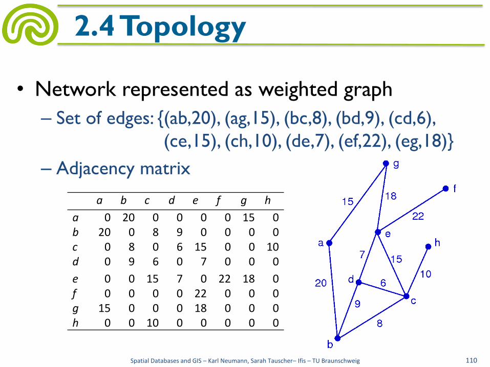
• Network represented as weighted graph
– Set of edges: {(ab,20), (ag,15), (bc,8), (bd,9), (cd,6),
(ce,15), (ch,10), (de,7), (ef,22), (eg,18)}
– Adjacency matrix
Spatial Databases and GIS – Karl Neumann, Sarah Tauscher– Ifis – TU Braunschweig 110
2.4 Topology
0 0 0 0 0 10 0 0 h 0 0 0 18 0 0 0 15 g 0 0 0 22 0 0 0 0 f 0 18 22 0 7 15 0 0 e
0 0 0 7 0 6 9 0 d 10 0 0 15 6 0 8 0 c
0 0 0 0 9 8 0 20 b 0 15 0 0 0 0 20 0 a
h g f e d c b a
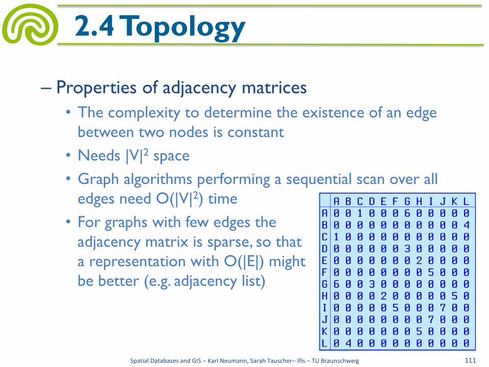
– Properties of adjacency matrices
• The complexity to determine the existence of an edge
between two nodes is constant
• Needs |V|2 space
• Graph algorithms performing a sequential scan over all
edges need O(|V|2) time
• For graphs with few edges the
adjacency matrix is sparse, so that
a representation with O(|E|) might
be better (e.g. adjacency list)
Spatial Databases and GIS – Karl Neumann, Sarah Tauscher– Ifis – TU Braunschweig 111
2.4 Topology
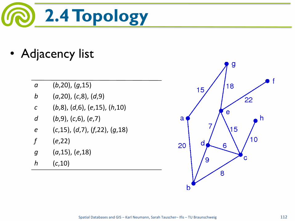
• Adjacency list
Spatial Databases and GIS – Karl Neumann, Sarah Tauscher– Ifis – TU Braunschweig 112
2.4 Topology
(c,10) h
(a,15), (e,18) g
(e,22) f
(c,15), (d,7), (f,22), (g,18) e
(b,9), (c,6), (e,7) d
(b,8), (d,6), (e,15), (h,10) c
(a,20), (c,8), (d,9) b
(b,20), (g,15) a
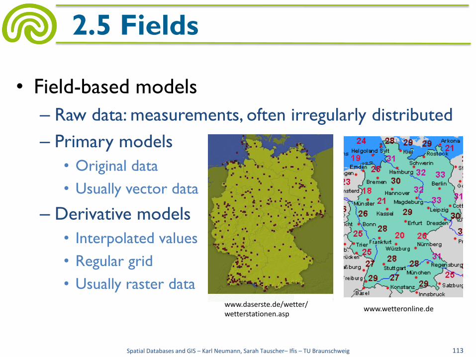
• Field-based models
– Raw data: measurements, often irregularly distributed
– Primary models
• Original data
• Usually vector data
– Derivative models
• Interpolated values
• Regular grid
• Usually raster data
Spatial Databases and GIS – Karl Neumann, Sarah Tauscher– Ifis – TU Braunschweig 113
2.5 Fields
www.wetteronline.de www.daserste.de/wetter/ wetterstationen.asp
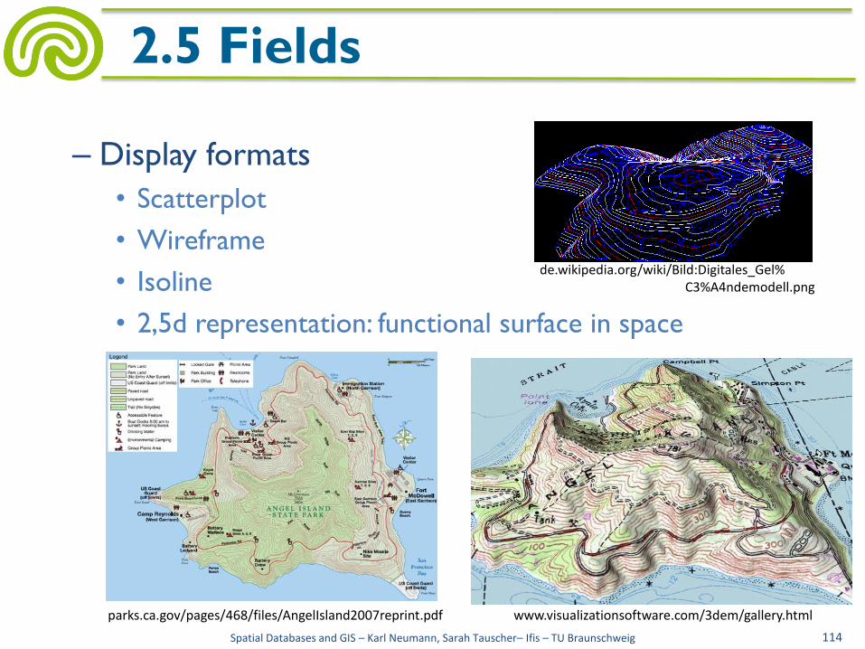
– Display formats
• Scatterplot
• Wireframe
• Isoline
• 2,5d representation: functional surface in space
Spatial Databases and GIS – Karl Neumann, Sarah Tauscher– Ifis – TU Braunschweig 114
2.5 Fields
parks.ca.gov/pages/468/files/AngelIsland2007reprint.pdf www.visualizationsoftware.com/3dem/gallery.html
de.wikipedia.org/wiki/Bild:Digitales_Gel% C3%A4ndemodell.png
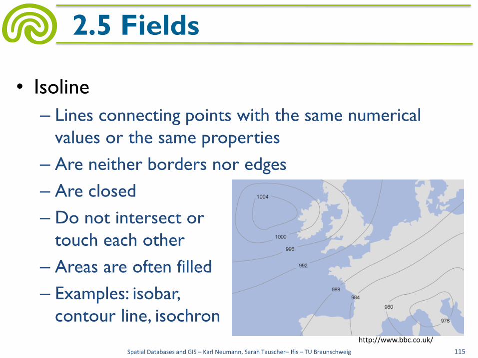
• Isoline
– Lines connecting points with the same numerical
values or the same properties
– Are neither borders nor edges
– Are closed
– Do not intersect or
touch each other
– Areas are often filled
– Examples: isobar,
contour line, isochron
Spatial Databases and GIS – Karl Neumann, Sarah Tauscher– Ifis – TU Braunschweig 115
2.5 Fields
http://www.bbc.co.uk/
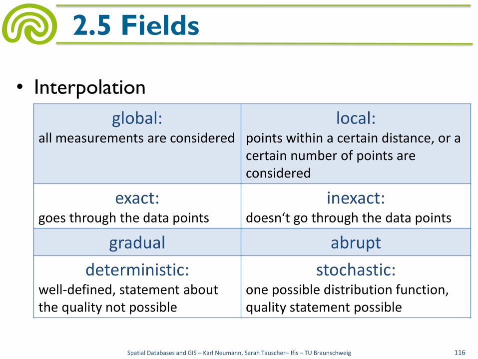
• Interpolation
Spatial Databases and GIS – Karl Neumann, Sarah Tauscher– Ifis – TU Braunschweig 116
2.5 Fields
global: all measurements are considered
local: points within a certain distance, or a certain number of points are considered
exact: goes through the data points
inexact: doesn‘t go through the data points
gradual abrupt
deterministic: well-defined, statement about the quality not possible
stochastic: one possible distribution function, quality statement possible
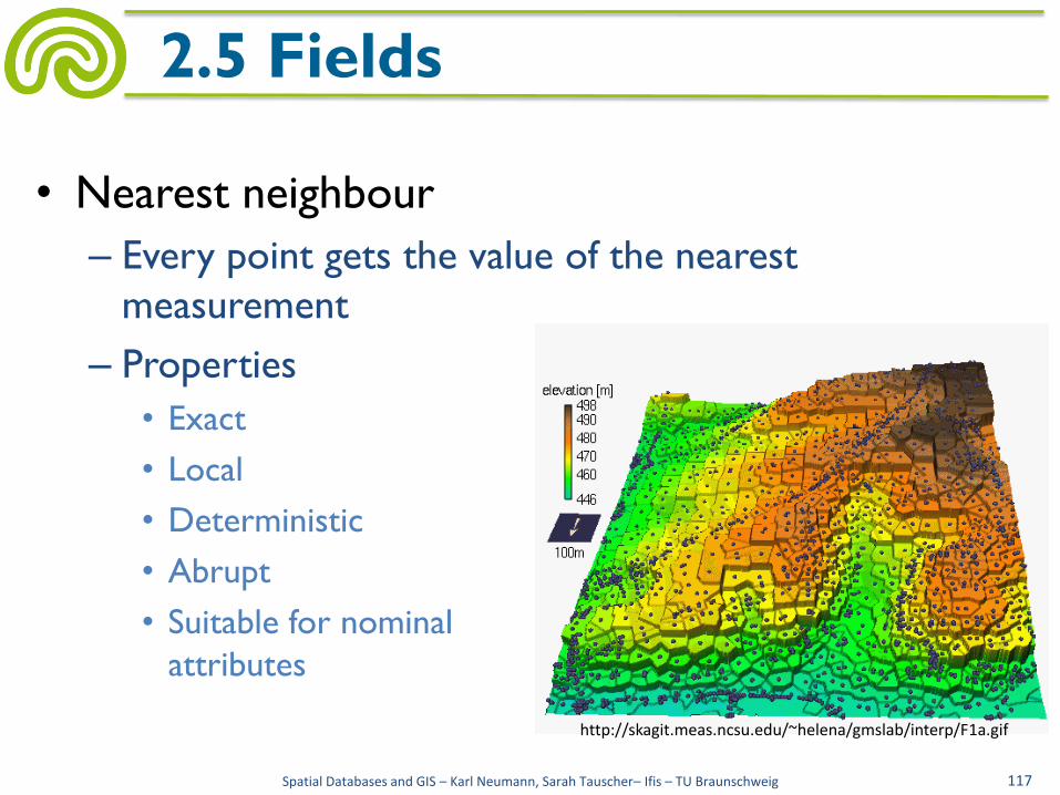
• Nearest neighbour
– Every point gets the value of the nearest
measurement
– Properties
• Exact
• Local
• Deterministic
• Abrupt
• Suitable for nominal
attributes
Spatial Databases and GIS – Karl Neumann, Sarah Tauscher– Ifis – TU Braunschweig 117
2.5 Fields
http://skagit.meas.ncsu.edu/~helena/gmslab/interp/F1a.gif
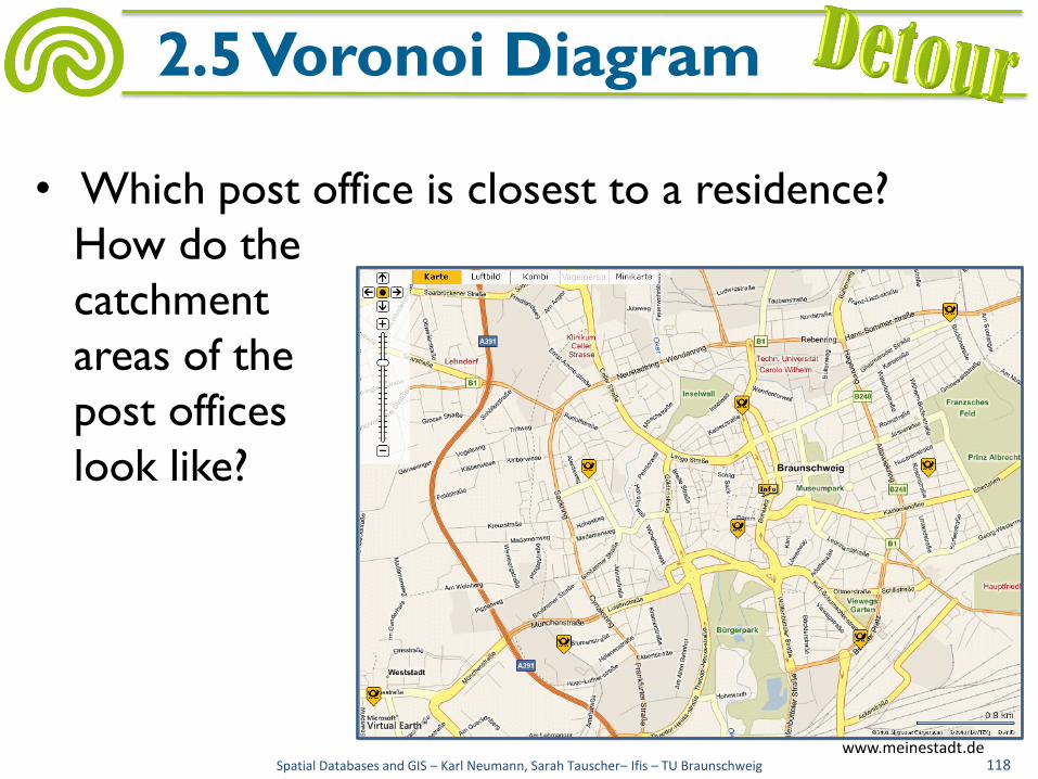
• Which post office is closest to a residence?
How do the
catchment
areas of the
post offices
look like?
Spatial Databases and GIS – Karl Neumann, Sarah Tauscher– Ifis – TU Braunschweig 118
2.5 Voronoi Diagram
www.meinestadt.de
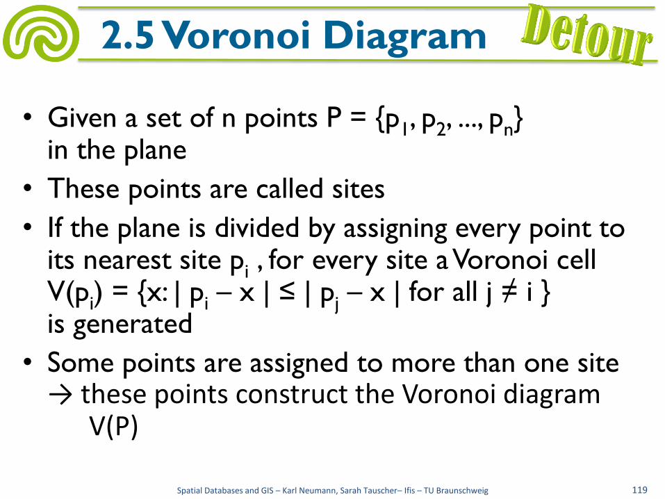
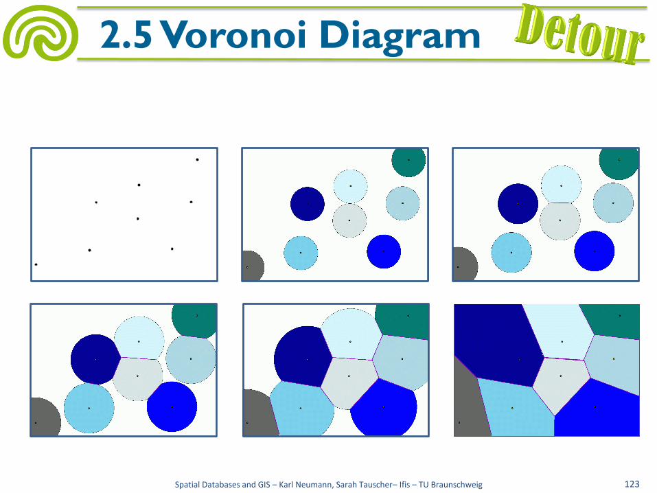
• Given a set of n points P = {p1, p2, ..., pn} in the plane
• These points are called sites
• If the plane is divided by assigning every point to its nearest site pi , for every site a Voronoi cell V(pi) = {x: | pi – x | ≤ | pj – x | for all j ≠ i } is generated
• Some points are assigned to more than one site → these points construct the Voronoi diagram V(P)
Spatial Databases and GIS – Karl Neumann, Sarah Tauscher– Ifis – TU Braunschweig 119
2.5 Voronoi Diagram
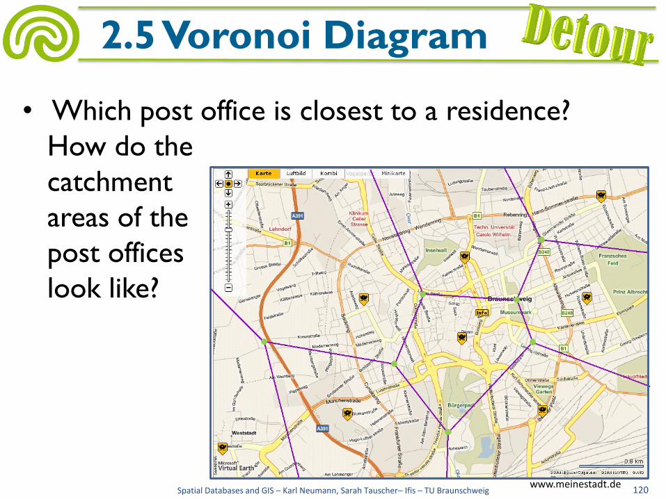
• Which post office is closest to a residence?
How do the
catchment
areas of the
post offices
look like?
Spatial Databases and GIS – Karl Neumann, Sarah Tauscher– Ifis – TU Braunschweig 120
2.5 Voronoi Diagram
www.meinestadt.de
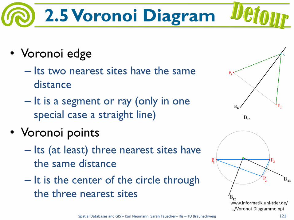
• Voronoi edge
– Its two nearest sites have the same
distance
– It is a segment or ray (only in one
special case a straight line)
• Voronoi points
– Its (at least) three nearest sites have
the same distance
– It is the center of the circle through
the three nearest sites
Spatial Databases and GIS – Karl Neumann, Sarah Tauscher– Ifis – TU Braunschweig 121
2.5 Voronoi Diagram
www.informatik.uni-trier.de/ .../Voronoi-Diagramme.ppt
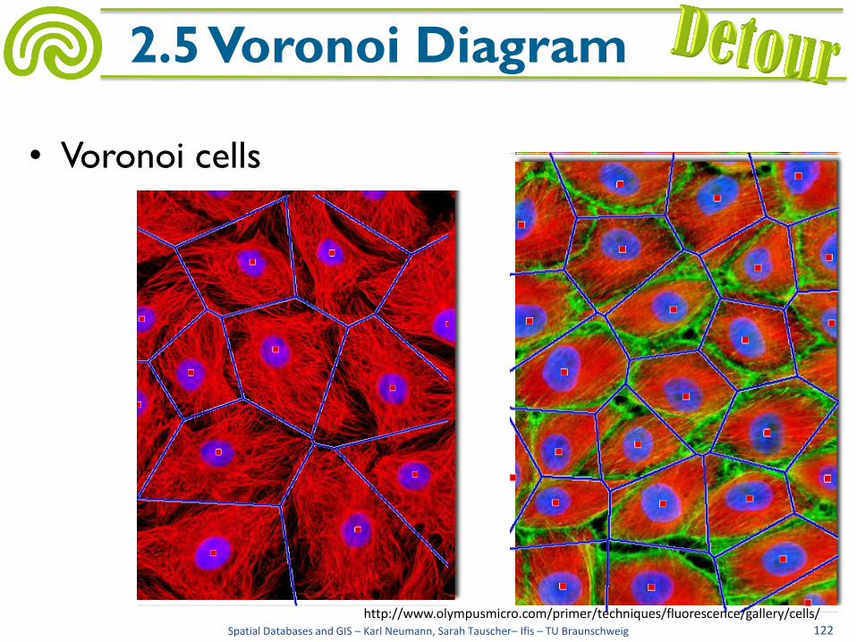
• Voronoi cells
Spatial Databases and GIS – Karl Neumann, Sarah Tauscher– Ifis – TU Braunschweig 122
2.5 Voronoi Diagram
http://www.olympusmicro.com/primer/techniques/fluorescence/gallery/cells/
Spatial Databases and GIS – Karl Neumann, Sarah Tauscher– Ifis – TU Braunschweig 123
2.5 Voronoi Diagram
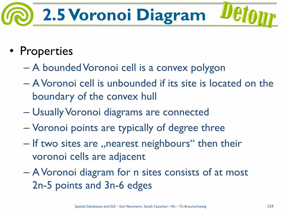
• Properties
– A bounded Voronoi cell is a convex polygon
– A Voronoi cell is unbounded if its site is located on the
boundary of the convex hull
– Usually Voronoi diagrams are connected
– Voronoi points are typically of degree three
– If two sites are „nearest neighbours“ then their
voronoi cells are adjacent
– A Voronoi diagram for n sites consists of at most
2n-5 points and 3n-6 edges
Spatial Databases and GIS – Karl Neumann, Sarah Tauscher– Ifis – TU Braunschweig 124
2.5 Voronoi Diagram
Spatial Databases and GIS – Karl Neumann, Sarah Tauscher– Ifis – TU Braunschweig 125
2.5 Voronoi Diagram
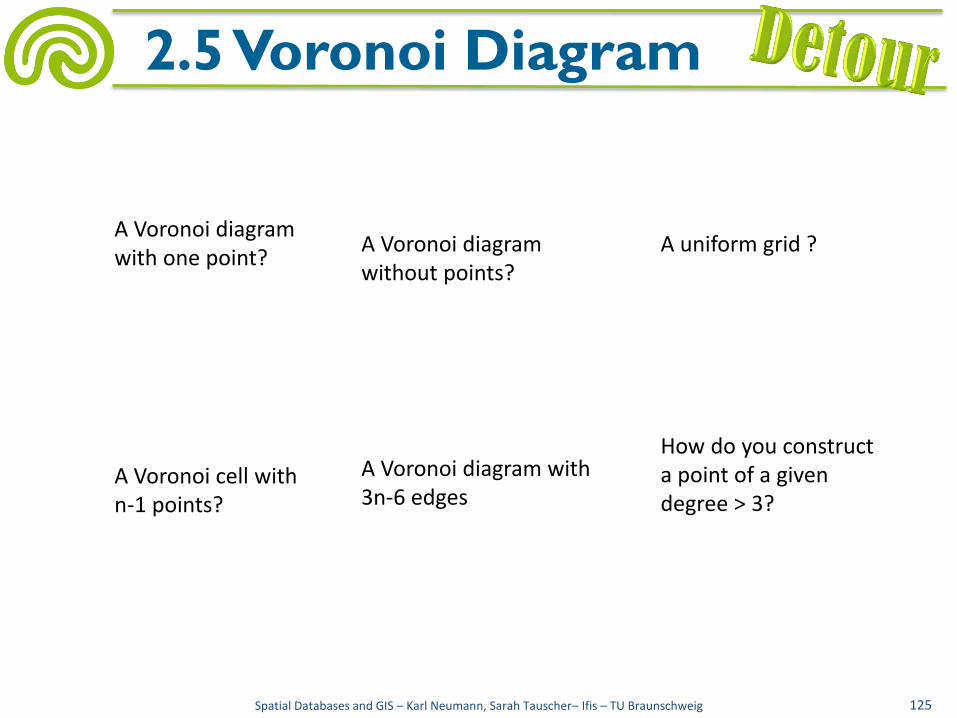
A Voronoi diagram with one point?
A Voronoi cell with n-1 points?
A Voronoi diagram without points?
A uniform grid ?
How do you construct a point of a given degree > 3?
A Voronoi diagram with 3n-6 edges
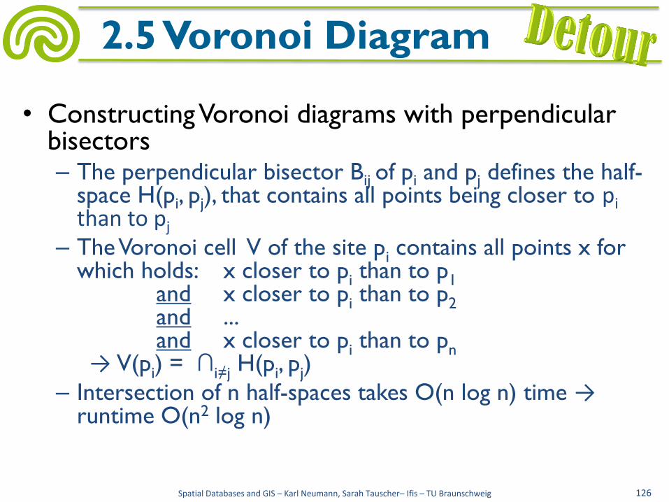
• Constructing Voronoi diagrams with perpendicular bisectors – The perpendicular bisector Bij of pi and pj defines the half-
space H(pi, pj), that contains all points being closer to pi than to pj
– The Voronoi cell V of the site pi contains all points x for which holds: x closer to pi than to p1 and x closer to pi than to p2 and ... and x closer to pi than to pn → V(pi) = ∩i≠j H(pi, pj)
– Intersection of n half-spaces takes O(n log n) time → runtime O(n2 log n)
Spatial Databases and GIS – Karl Neumann, Sarah Tauscher– Ifis – TU Braunschweig 126
2.5 Voronoi Diagram
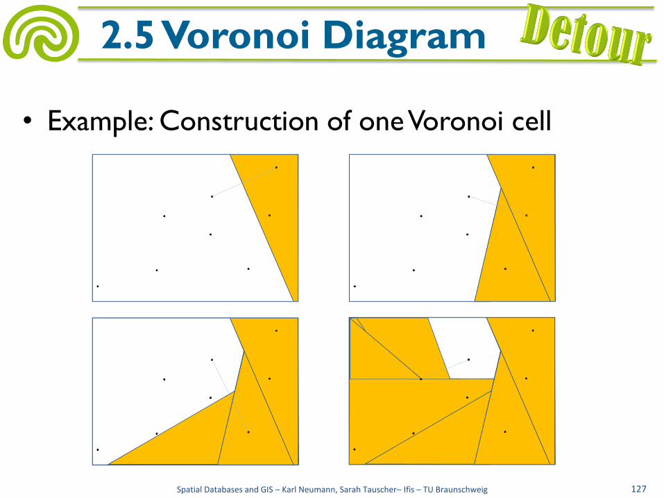
• Example: Construction of one Voronoi cell
Spatial Databases and GIS – Karl Neumann, Sarah Tauscher– Ifis – TU Braunschweig 127
2.5 Voronoi Diagram
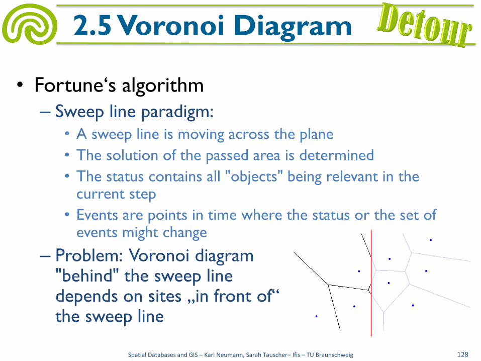
• Fortune‘s algorithm
– Sweep line paradigm:
• A sweep line is moving across the plane
• The solution of the passed area is determined
• The status contains all "objects" being relevant in the current step
• Events are points in time where the status or the set of events might change
– Problem: Voronoi diagram "behind" the sweep line depends on sites „in front of“ the sweep line
Spatial Databases and GIS – Karl Neumann, Sarah Tauscher– Ifis – TU Braunschweig 128
2.5 Voronoi Diagram
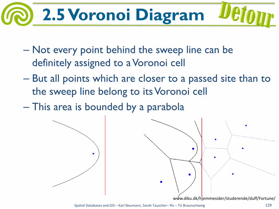
– Not every point behind the sweep line can be
definitely assigned to a Voronoi cell
– But all points which are closer to a passed site than to
the sweep line belong to its Voronoi cell
– This area is bounded by a parabola
Spatial Databases and GIS – Karl Neumann, Sarah Tauscher– Ifis – TU Braunschweig 129
2.5 Voronoi Diagram
www.diku.dk/hjemmesider/studerende/duff/Fortune/
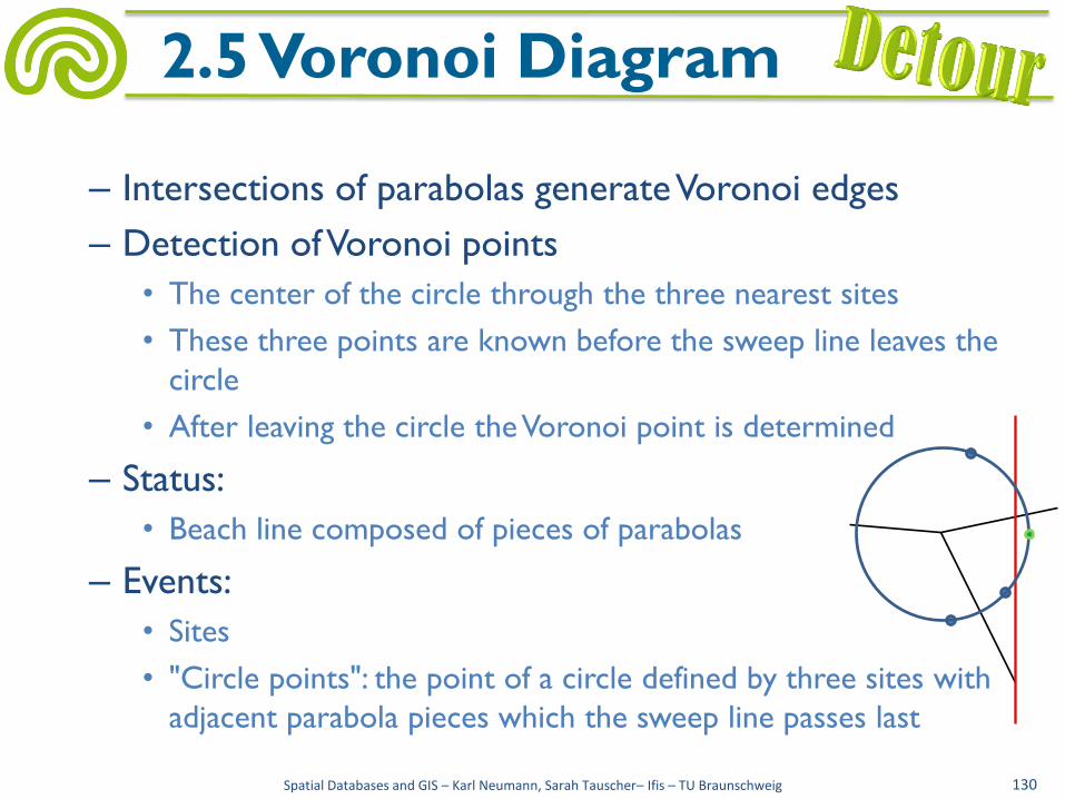
– Intersections of parabolas generate Voronoi edges
– Detection of Voronoi points
• The center of the circle through the three nearest sites
• These three points are known before the sweep line leaves the
circle
• After leaving the circle the Voronoi point is determined
– Status:
• Beach line composed of pieces of parabolas
– Events:
• Sites
• "Circle points": the point of a circle defined by three sites with
adjacent parabola pieces which the sweep line passes last
Spatial Databases and GIS – Karl Neumann, Sarah Tauscher– Ifis – TU Braunschweig 130
2.5 Voronoi Diagram
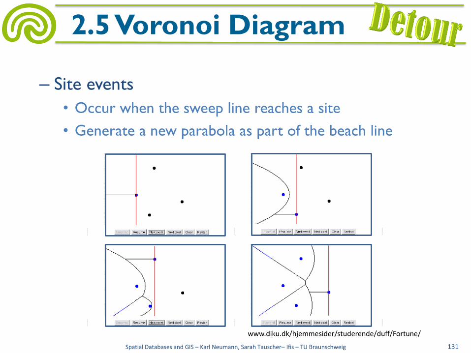
– Site events
• Occur when the sweep line reaches a site
• Generate a new parabola as part of the beach line
Spatial Databases and GIS – Karl Neumann, Sarah Tauscher– Ifis – TU Braunschweig 131
2.5 Voronoi Diagram
www.diku.dk/hjemmesider/studerende/duff/Fortune/
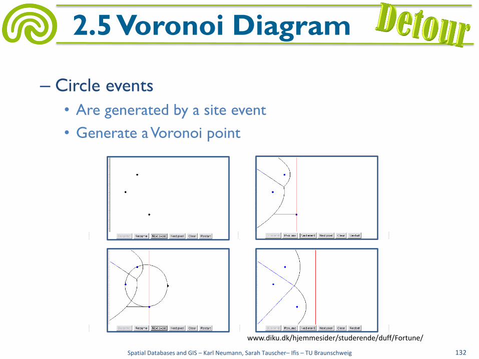
– Circle events
• Are generated by a site event
• Generate a Voronoi point
Spatial Databases and GIS – Karl Neumann, Sarah Tauscher– Ifis – TU Braunschweig 132
2.5 Voronoi Diagram
www.diku.dk/hjemmesider/studerende/duff/Fortune/
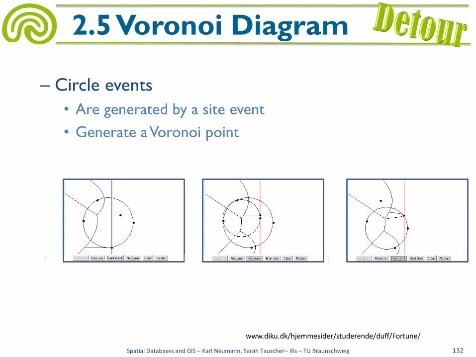
– Circle events
• Are generated by a site event
• Generate a Voronoi point
Spatial Databases and GIS – Karl Neumann, Sarah Tauscher– Ifis – TU Braunschweig 132
2.5 Voronoi Diagram
www.diku.dk/hjemmesider/studerende/duff/Fortune/
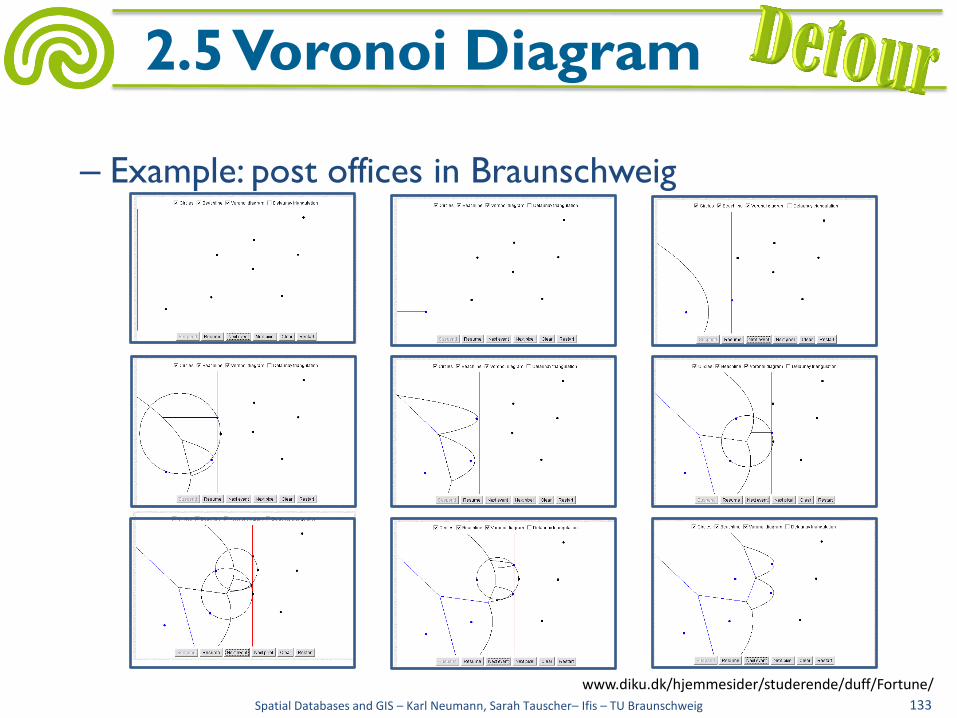
– Example: post offices in Braunschweig
Spatial Databases and GIS – Karl Neumann, Sarah Tauscher– Ifis – TU Braunschweig 133
2.5 Voronoi Diagram
www.diku.dk/hjemmesider/studerende/duff/Fortune/
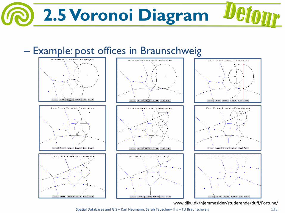
– Example: post offices in Braunschweig
Spatial Databases and GIS – Karl Neumann, Sarah Tauscher– Ifis – TU Braunschweig 133
2.5 Voronoi Diagram
www.diku.dk/hjemmesider/studerende/duff/Fortune/
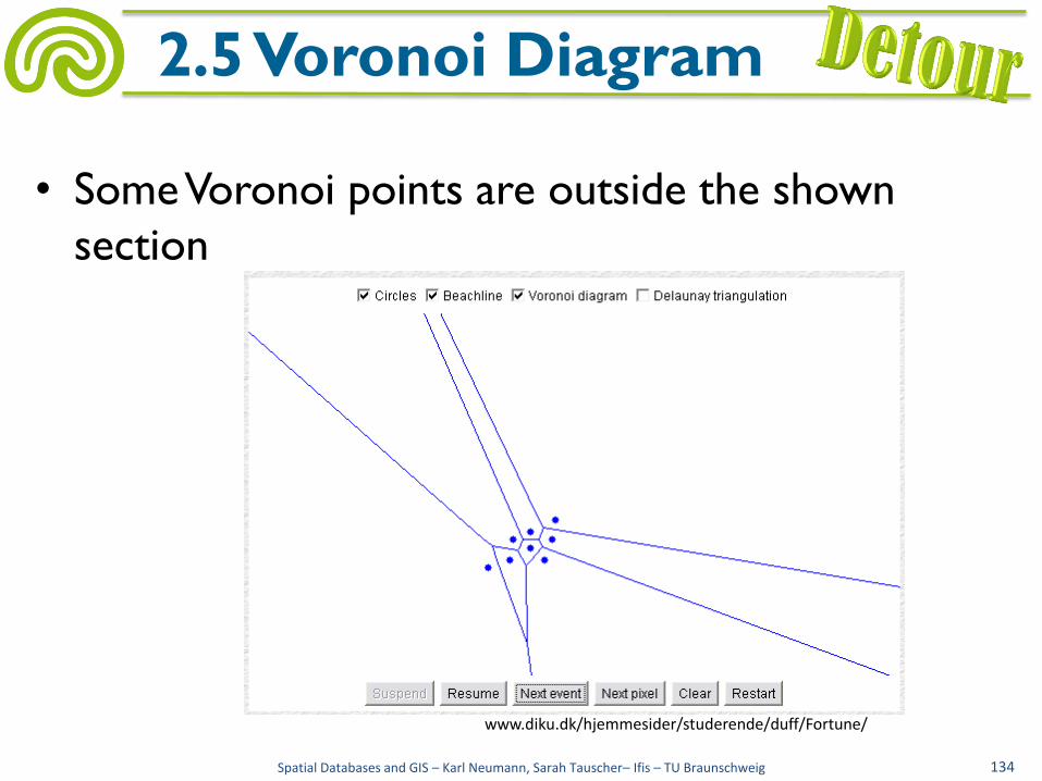
• Some Voronoi points are outside the shown
section
Spatial Databases and GIS – Karl Neumann, Sarah Tauscher– Ifis – TU Braunschweig 134
2.5 Voronoi Diagram
www.diku.dk/hjemmesider/studerende/duff/Fortune/
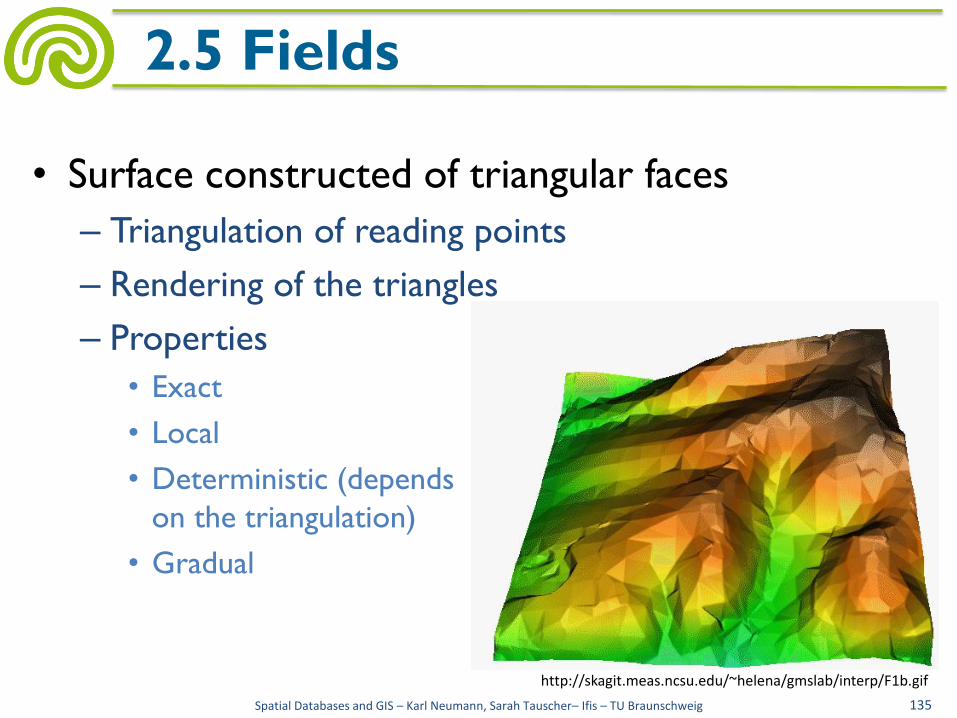
• Surface constructed of triangular faces
– Triangulation of reading points
– Rendering of the triangles
– Properties
• Exact
• Local
• Deterministic (depends
on the triangulation)
• Gradual
Spatial Databases and GIS – Karl Neumann, Sarah Tauscher– Ifis – TU Braunschweig 135
2.5 Fields
http://skagit.meas.ncsu.edu/~helena/gmslab/interp/F1b.gif
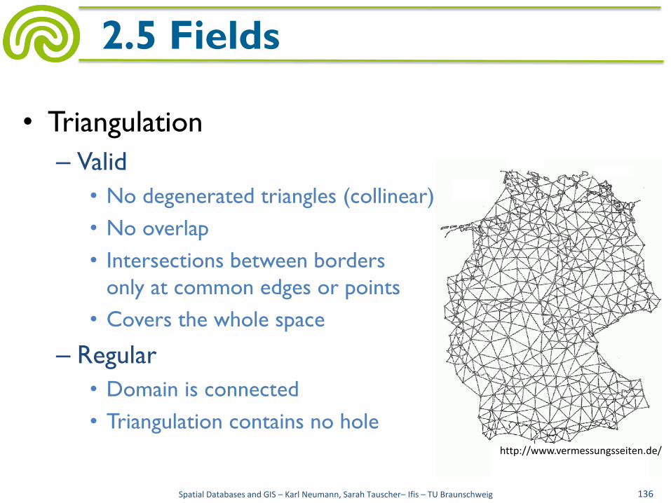
• Triangulation
– Valid
• No degenerated triangles (collinear)
• No overlap
• Intersections between borders
only at common edges or points
• Covers the whole space
– Regular
• Domain is connected
• Triangulation contains no hole
Spatial Databases and GIS – Karl Neumann, Sarah Tauscher– Ifis – TU Braunschweig 136
2.5 Fields
http://www.vermessungsseiten.de/
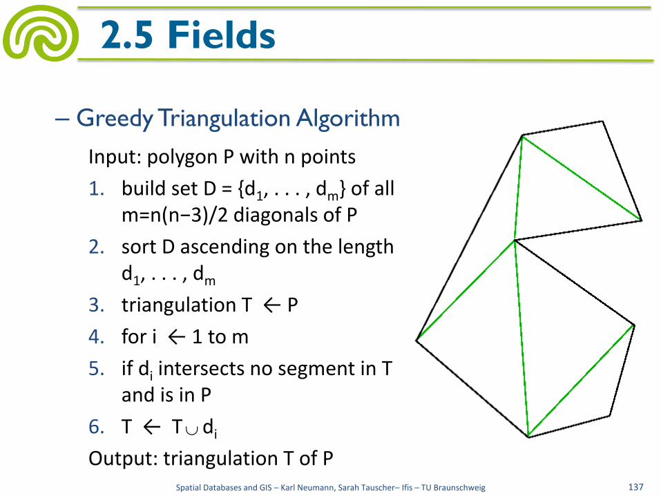
– Greedy Triangulation Algorithm
Spatial Databases and GIS – Karl Neumann, Sarah Tauscher– Ifis – TU Braunschweig 137
2.5 Fields
Input: polygon P with n points
1. build set D = {d1, . . . , dm} of all m=n(n−3)/2 diagonals of P
2. sort D ascending on the length d1, . . . , dm
3. triangulation T ← P
4. for i ← 1 to m
5. if di intersects no segment in T and is in P
6. T ← T di
Output: triangulation T of P
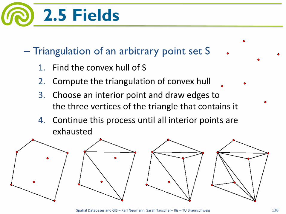
– Triangulation of an arbitrary point set S
Spatial Databases and GIS – Karl Neumann, Sarah Tauscher– Ifis – TU Braunschweig 138
2.5 Fields
1. Find the convex hull of S
2. Compute the triangulation of convex hull 3. Choose an interior point and draw edges to
the three vertices of the triangle that contains it
4. Continue this process until all interior points are exhausted
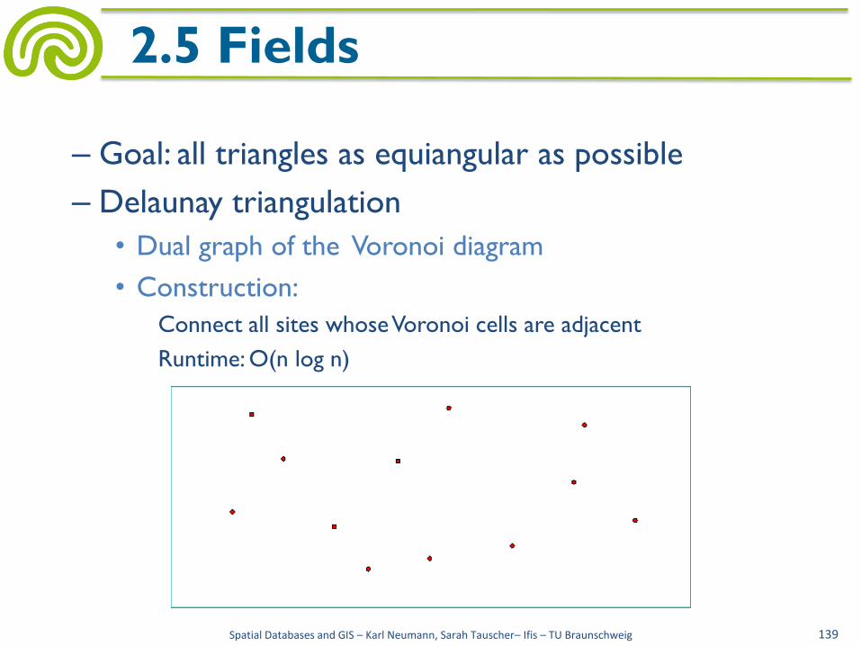
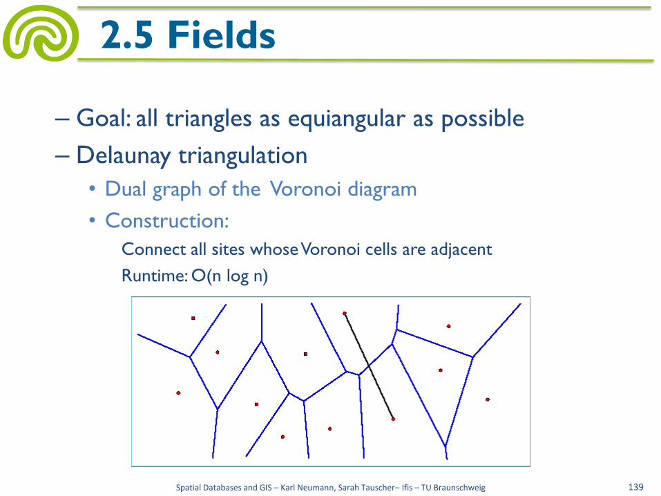
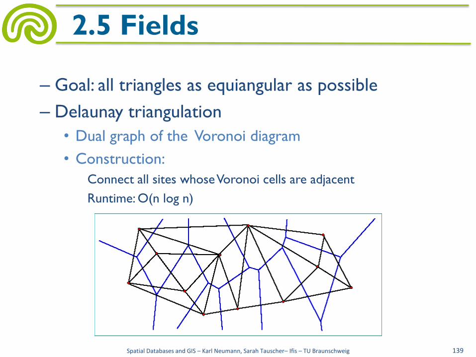
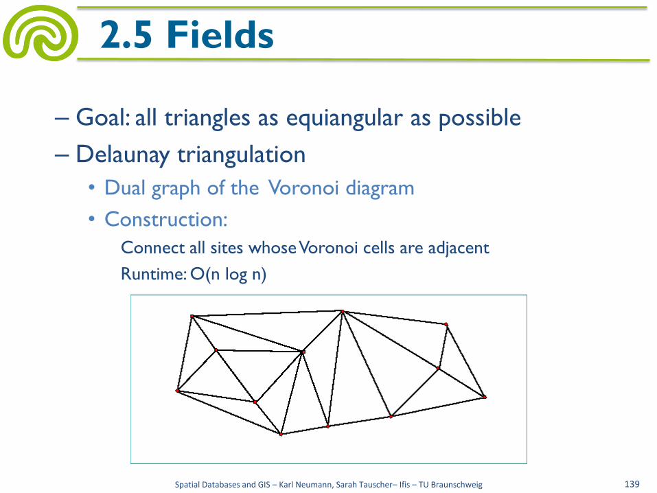
– Goal: all triangles as equiangular as possible
– Delaunay triangulation
• Dual graph of the Voronoi diagram
• Construction:
Connect all sites whose Voronoi cells are adjacent
Runtime: O(n log n)
Spatial Databases and GIS – Karl Neumann, Sarah Tauscher– Ifis – TU Braunschweig 139
2.5 Fields
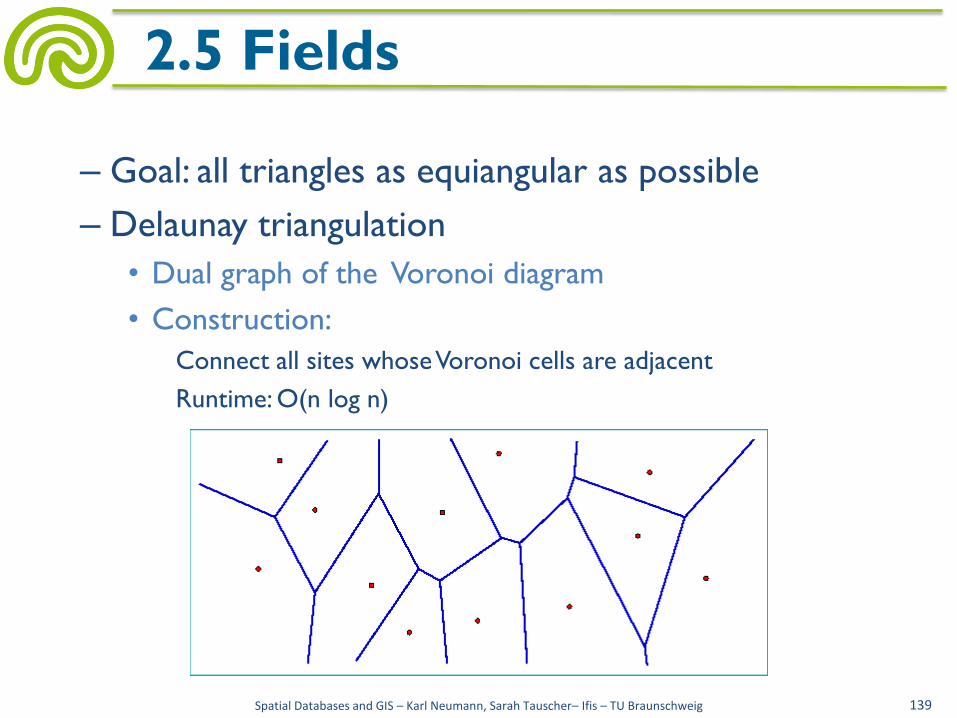
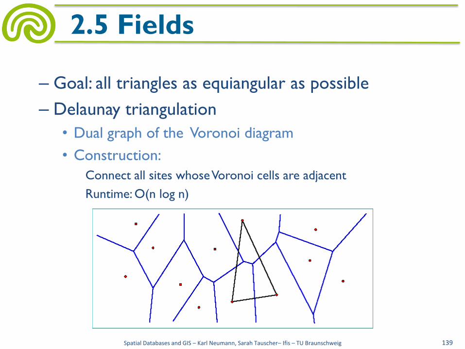
– Goal: all triangles as equiangular as possible
– Delaunay triangulation
• Dual graph of the Voronoi diagram
• Construction:
Connect all sites whose Voronoi cells are adjacent
Runtime: O(n log n)
Spatial Databases and GIS – Karl Neumann, Sarah Tauscher– Ifis – TU Braunschweig 139
2.5 Fields
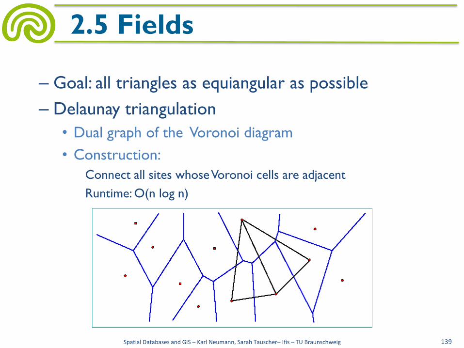
– Goal: all triangles as equiangular as possible
– Delaunay triangulation
• Dual graph of the Voronoi diagram
• Construction:
Connect all sites whose Voronoi cells are adjacent
Runtime: O(n log n)
Spatial Databases and GIS – Karl Neumann, Sarah Tauscher– Ifis – TU Braunschweig 139
2.5 Fields

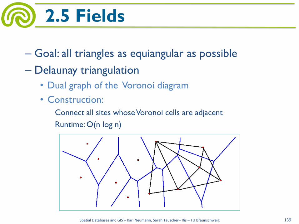
– Goal: all triangles as equiangular as possible
– Delaunay triangulation
• Dual graph of the Voronoi diagram
• Construction:
Connect all sites whose Voronoi cells are adjacent
Runtime: O(n log n)
Spatial Databases and GIS – Karl Neumann, Sarah Tauscher– Ifis – TU Braunschweig 139
2.5 Fields
– Goal: all triangles as equiangular as possible
– Delaunay triangulation
• Dual graph of the Voronoi diagram
• Construction:
Connect all sites whose Voronoi cells are adjacent
Runtime: O(n log n)
Spatial Databases and GIS – Karl Neumann, Sarah Tauscher– Ifis – TU Braunschweig 139
2.5 Fields
– Goal: all triangles as equiangular as possible
– Delaunay triangulation
• Dual graph of the Voronoi diagram
• Construction:
Connect all sites whose Voronoi cells are adjacent
Runtime: O(n log n)
Spatial Databases and GIS – Karl Neumann, Sarah Tauscher– Ifis – TU Braunschweig 139
2.5 Fields
– Goal: all triangles as equiangular as possible
– Delaunay triangulation
• Dual graph of the Voronoi diagram
• Construction:
Connect all sites whose Voronoi cells are adjacent
Runtime: O(n log n)
Spatial Databases and GIS – Karl Neumann, Sarah Tauscher– Ifis – TU Braunschweig 139
2.5 Fields
– Goal: all triangles as equiangular as possible
– Delaunay triangulation
• Dual graph of the Voronoi diagram
• Construction:
Connect all sites whose Voronoi cells are adjacent
Runtime: O(n log n)
Spatial Databases and GIS – Karl Neumann, Sarah Tauscher– Ifis – TU Braunschweig 139
2.5 Fields
– Goal: all triangles as equiangular as possible
– Delaunay triangulation
• Dual graph of the Voronoi diagram
• Construction:
Connect all sites whose Voronoi cells are adjacent
Runtime: O(n log n)
Spatial Databases and GIS – Karl Neumann, Sarah Tauscher– Ifis – TU Braunschweig 139
2.5 Fields
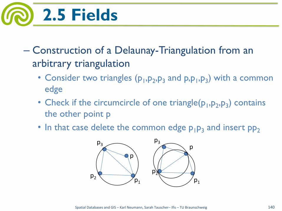
– Construction of a Delaunay-Triangulation from an
arbitrary triangulation
• Consider two triangles (p1,p2,p3 and p,p1,p3) with a common
edge
• Check if the circumcircle of one triangle(p1,p2,p3) contains
the other point p
• In that case delete the common edge p1p3 and insert pp2
Spatial Databases and GIS – Karl Neumann, Sarah Tauscher– Ifis – TU Braunschweig 140
2.5 Fields
p3 p3
p1 p2
p
p1 p2
p
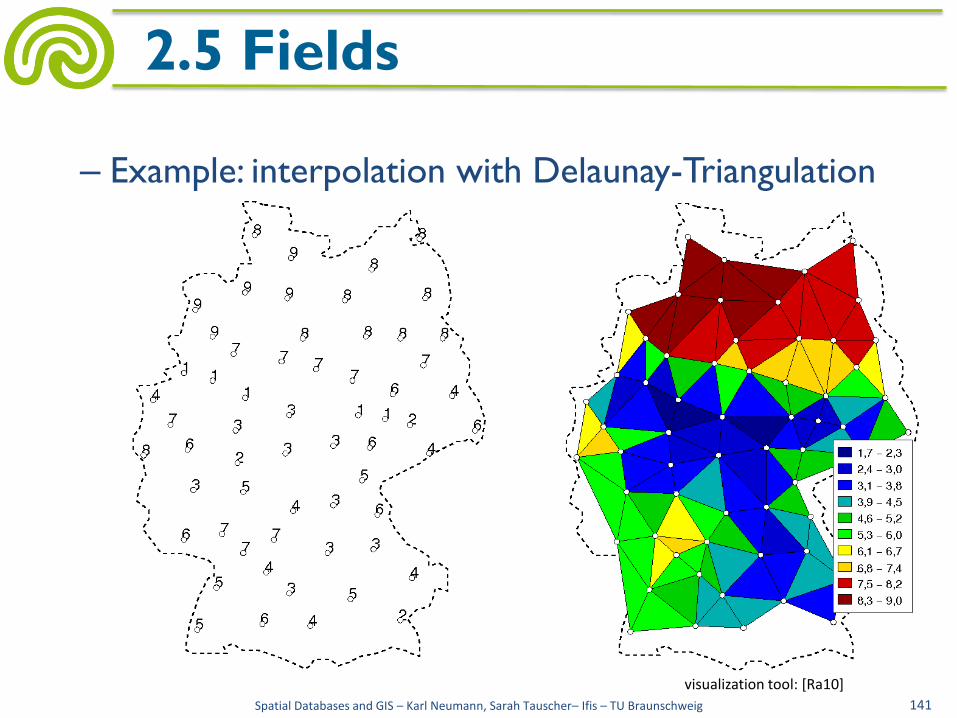
– Example: interpolation with Delaunay-Triangulation
Spatial Databases and GIS – Karl Neumann, Sarah Tauscher– Ifis – TU Braunschweig 141
2.5 Fields
visualization tool: [Ra10]
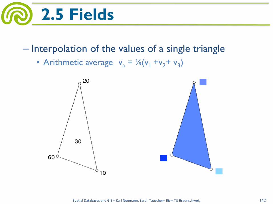
– Interpolation of the values of a single triangle
• Arithmetic average va = ⅓(v1 +v2+ v3)
Spatial Databases and GIS – Karl Neumann, Sarah Tauscher– Ifis – TU Braunschweig 142
2.5 Fields
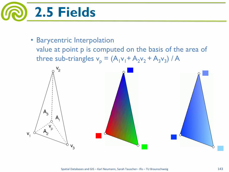
• Barycentric Interpolation
value at point p is computed on the basis of the area of
three sub-triangles vp = (A1v1+ A2v2 + A3v3) / A
Spatial Databases and GIS – Karl Neumann, Sarah Tauscher– Ifis – TU Braunschweig 143
2.5 Fields
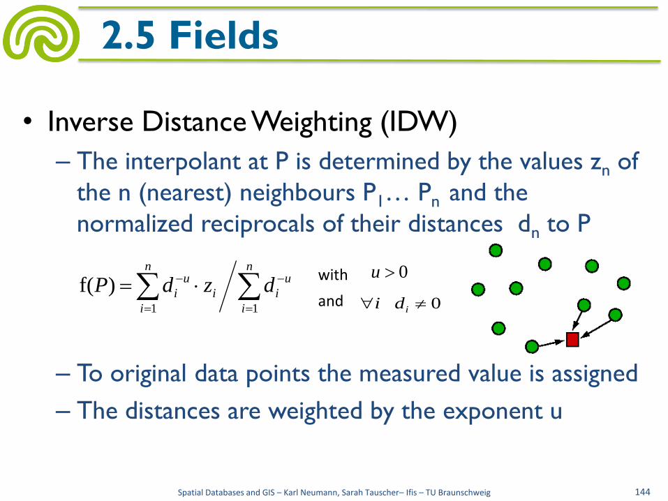
• Inverse Distance Weighting (IDW)
– The interpolant at P is determined by the values zn of
the n (nearest) neighbours P1… Pn and the
normalized reciprocals of their distances dn to P
– To original data points the measured value is assigned
– The distances are weighted by the exponent u
Spatial Databases and GIS – Karl Neumann, Sarah Tauscher– Ifis – TU Braunschweig 144
2.5 Fields
n
i
u
i
n
i
i
u
i dzdP11
)f(0uwith
and 0 idi
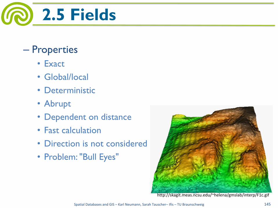
– Properties
• Exact
• Global/local
• Deterministic
• Abrupt
• Dependent on distance
• Fast calculation
• Direction is not considered
• Problem: "Bull Eyes"
Spatial Databases and GIS – Karl Neumann, Sarah Tauscher– Ifis – TU Braunschweig 145
2.5 Fields
http://skagit.meas.ncsu.edu/~helena/gmslab/interp/F1c.gif
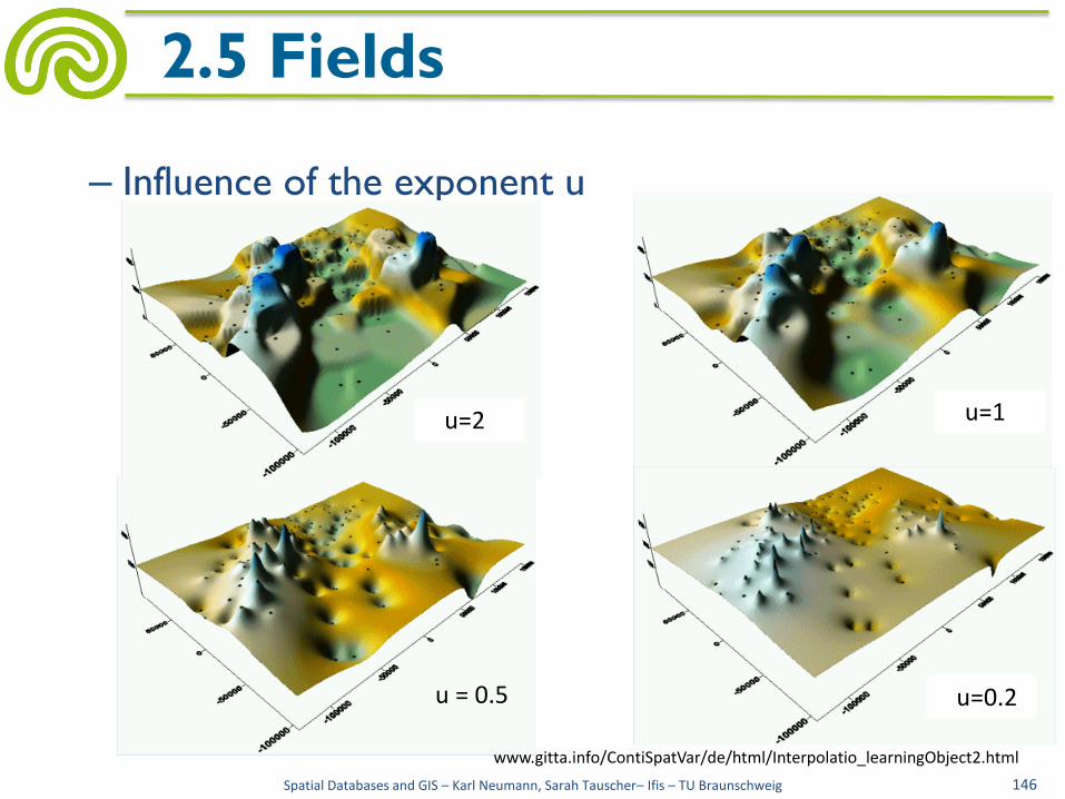
– Influence of the exponent u
Spatial Databases and GIS – Karl Neumann, Sarah Tauscher– Ifis – TU Braunschweig 146
2.5 Fields
www.gitta.info/ContiSpatVar/de/html/Interpolatio_learningObject2.html
u = 0.5
u = 0.5
u = 1
u = 5
u=2 u=1
u=0.2
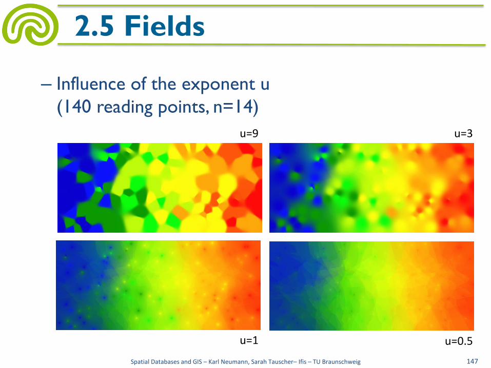
– Influence of the exponent u
(140 reading points, n=14)
Spatial Databases and GIS – Karl Neumann, Sarah Tauscher– Ifis – TU Braunschweig 147
2.5 Fields
u=9 u=3
u=1 u=0.5
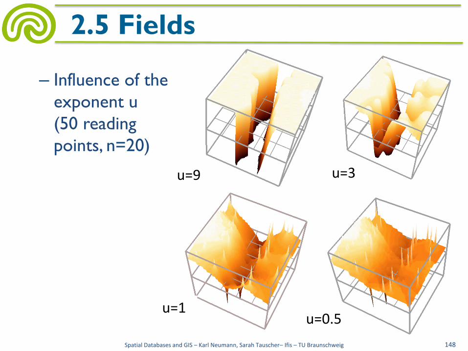
– Influence of the
exponent u
(50 reading
points, n=20)
Spatial Databases and GIS – Karl Neumann, Sarah Tauscher– Ifis – TU Braunschweig 148
2.5 Fields
u=9 u=3
u=0.5 u=1
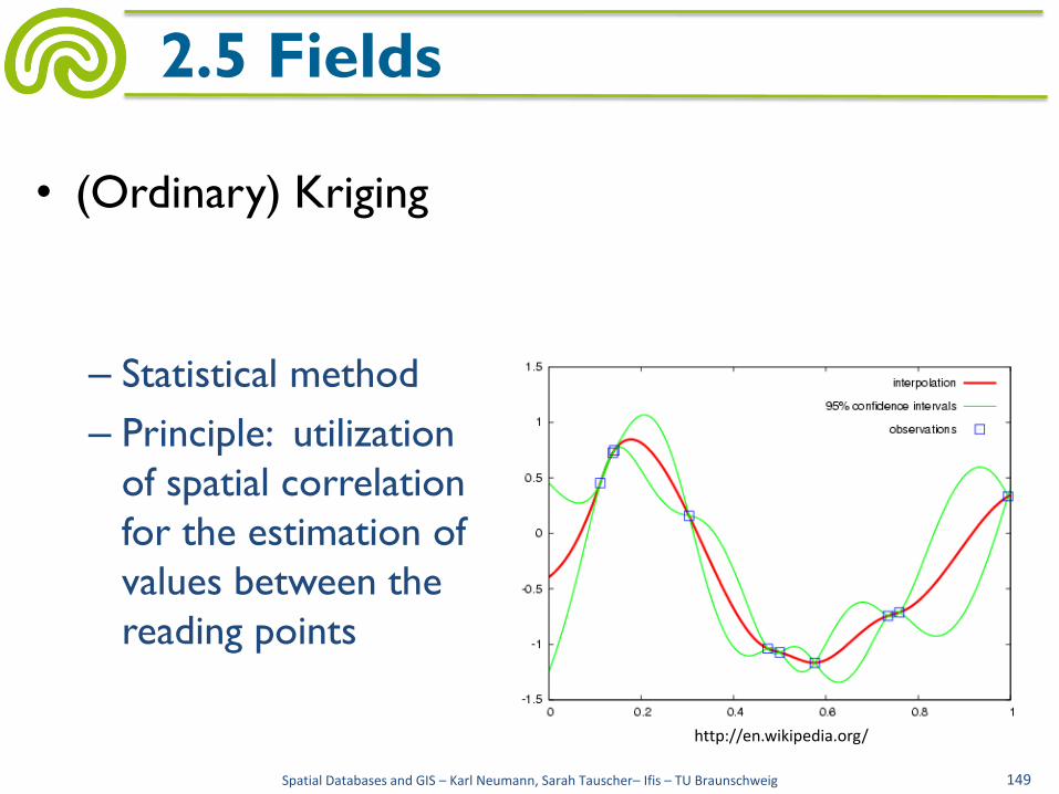
• (Ordinary) Kriging
– Statistical method
– Principle: utilization
of spatial correlation
for the estimation of
values between the
reading points
Spatial Databases and GIS – Karl Neumann, Sarah Tauscher– Ifis – TU Braunschweig 149
2.5 Fields
http://en.wikipedia.org/
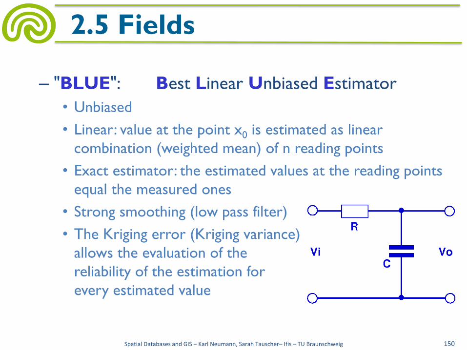
– "BLUE": Best Linear Unbiased Estimator
• Unbiased
• Linear: value at the point x0 is estimated as linear
combination (weighted mean) of n reading points
• Exact estimator: the estimated values at the reading points
equal the measured ones
• Strong smoothing (low pass filter)
• The Kriging error (Kriging variance)
allows the evaluation of the
reliability of the estimation for
every estimated value
Spatial Databases and GIS – Karl Neumann, Sarah Tauscher– Ifis – TU Braunschweig 150
2.5 Fields
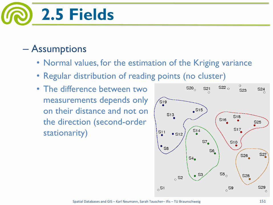
– Assumptions
• Normal values, for the estimation of the Kriging variance
• Regular distribution of reading points (no cluster)
• The difference between two
measurements depends only
on their distance and not on
the direction (second-order
stationarity)
Spatial Databases and GIS – Karl Neumann, Sarah Tauscher– Ifis – TU Braunschweig 151
2.5 Fields
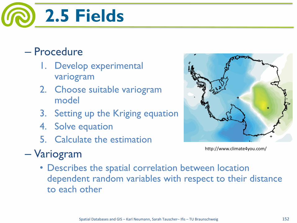
– Procedure
1. Develop experimental variogram
2. Choose suitable variogram model
3. Setting up the Kriging equation
4. Solve equation
5. Calculate the estimation
– Variogram
• Describes the spatial correlation between location dependent random variables with respect to their distance to each other
Spatial Databases and GIS – Karl Neumann, Sarah Tauscher– Ifis – TU Braunschweig 152
2.5 Fields
http://www.climate4you.com/
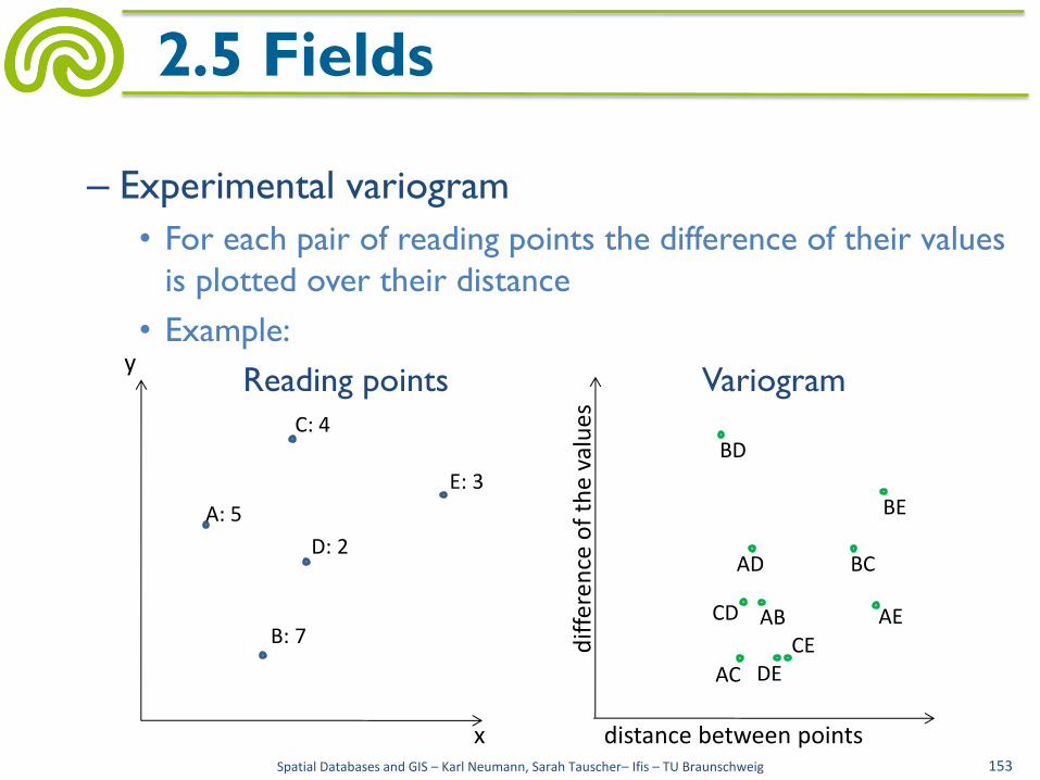
– Experimental variogram
• For each pair of reading points the difference of their values
is plotted over their distance
• Example:
Reading points Variogram
Spatial Databases and GIS – Karl Neumann, Sarah Tauscher– Ifis – TU Braunschweig 153
2.5 Fields
y
x
C: 4
E: 3
D: 2
A: 5
B: 7 dif
fere
nce
of
the
val
ues
distance between points
CE
CD
DE
AD
AC
BD
AE AB
BE
BC
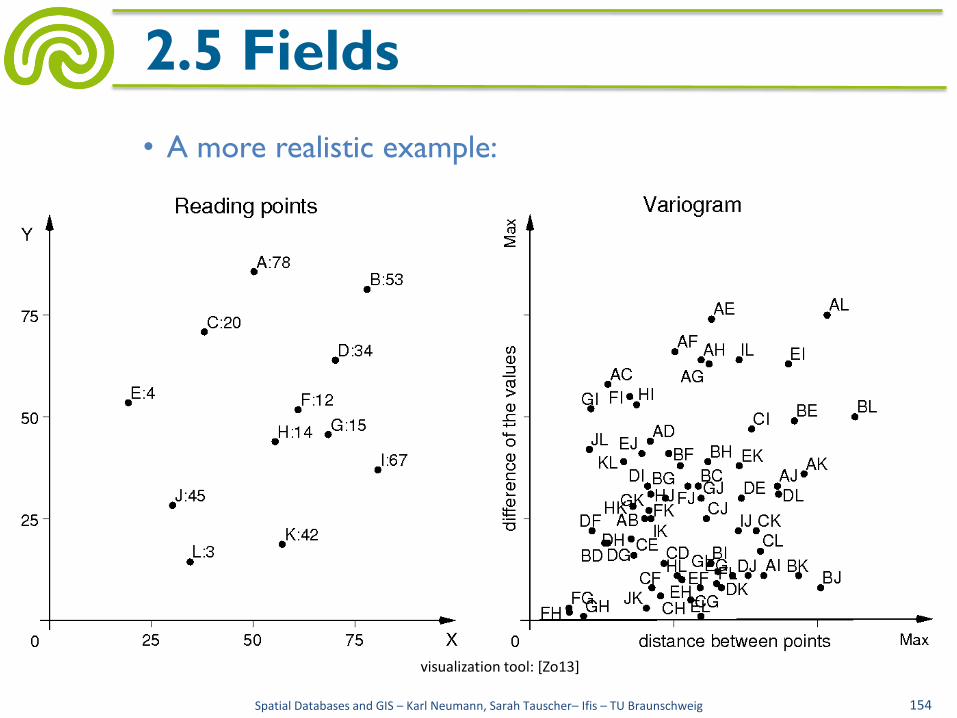
• A more realistic example:
Spatial Databases and GIS – Karl Neumann, Sarah Tauscher– Ifis – TU Braunschweig 154
2.5 Fields
visualization tool: [Zo13]
0.0
0.2
0.4
0.6
0.8
1.0
0 10 20 30 40 50
γ(h)
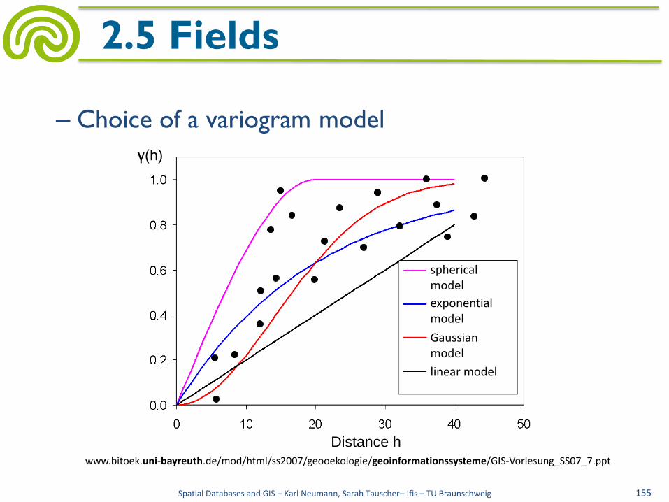
– Choice of a variogram model
Distance h
γ(h)
Spatial Databases and GIS – Karl Neumann, Sarah Tauscher– Ifis – TU Braunschweig 155
2.5 Fields
www.bitoek.uni-bayreuth.de/mod/html/ss2007/geooekologie/geoinformationssysteme/GIS-Vorlesung_SS07_7.ppt
spherical model
exponential model
Gaussian model
linear model
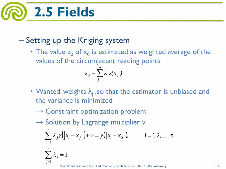
– Setting up the Kriging system
• The value z0 of x0 is estimated as weighted average of the
values of the circumjacent reading points
• Wanted: weights λj ,so that the estimator is unbiased and
the variance is minimized
→ Constraint optimization problem
→ Solution by Lagrange multiplier ν
Spatial Databases and GIS – Karl Neumann, Sarah Tauscher– Ifis – TU Braunschweig 156
2.5 Fields
n
j=
jj )z(xλ=z1
0
1
,,2,1,
1
0
1
n
j
j
i
n
j
jij nixxxx
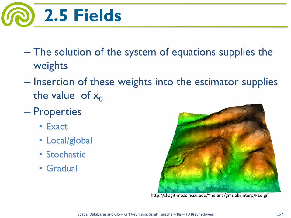
– The solution of the system of equations supplies the
weights
– Insertion of these weights into the estimator supplies
the value of x0
– Properties
• Exact
• Local/global
• Stochastic
• Gradual
Spatial Databases and GIS – Karl Neumann, Sarah Tauscher– Ifis – TU Braunschweig 157
2.5 Fields
http://skagit.meas.ncsu.edu/~helena/gmslab/interp/F1d.gif
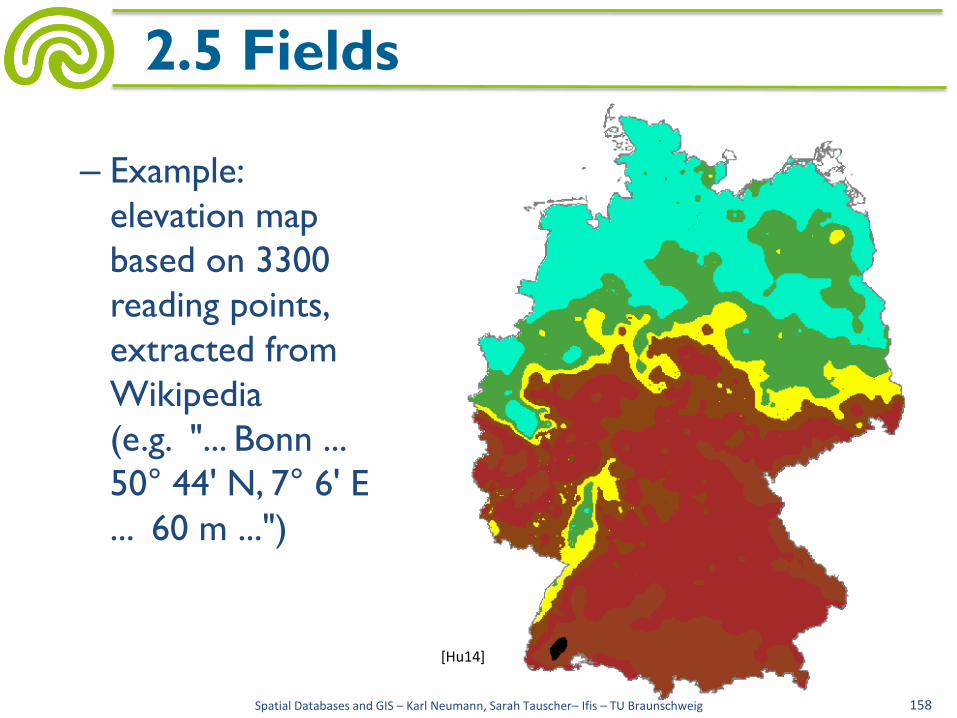
– Example:
elevation map
based on 3300
reading points,
extracted from
Wikipedia
(e.g. "... Bonn ...
50° 44' N, 7° 6' E
... 60 m ...")
Spatial Databases and GIS – Karl Neumann, Sarah Tauscher– Ifis – TU Braunschweig 158
2.5 Fields
[Hu14]
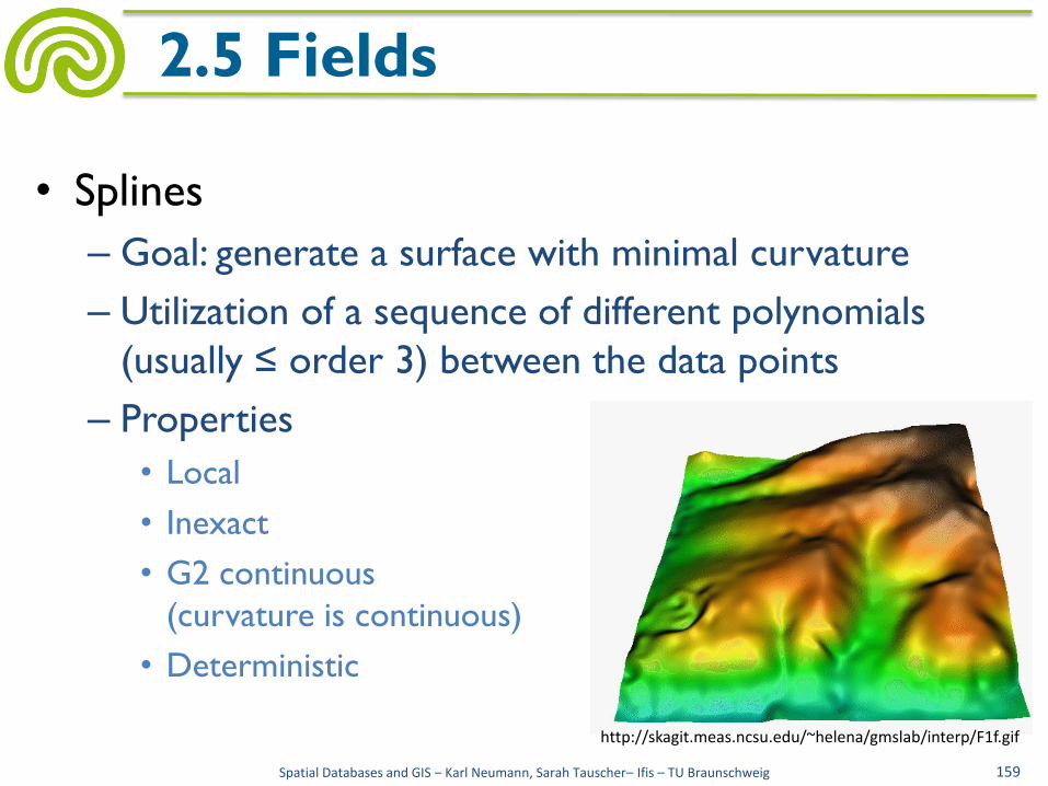
• Splines
– Goal: generate a surface with minimal curvature
– Utilization of a sequence of different polynomials
(usually ≤ order 3) between the data points
– Properties
• Local
• Inexact
• G2 continuous
(curvature is continuous)
• Deterministic
Spatial Databases and GIS – Karl Neumann, Sarah Tauscher– Ifis – TU Braunschweig 159
2.5 Fields
http://skagit.meas.ncsu.edu/~helena/gmslab/interp/F1f.gif
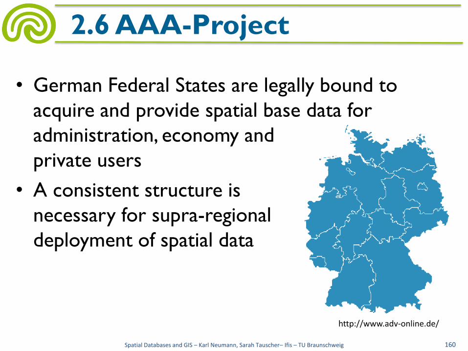
• German Federal States are legally bound to
acquire and provide spatial base data for
administration, economy and
private users
• A consistent structure is
necessary for supra-regional
deployment of spatial data
Spatial Databases and GIS – Karl Neumann, Sarah Tauscher– Ifis – TU Braunschweig 160
2.6 AAA-Project
http://www.adv-online.de/

• Working Committee of the Surveying Authorities
of the States of the Federal Republic of Germany
(AdV: Arbeitsgemeinschaft der
Vermessungsverwaltungen der Bundesländer)
– Members
• The Cadastral and Surveying
Authorities of the 16 German
Federal States
• Federal ministry of the Interior, of
Defense, and of Transport, Building
and Urban Affairs
Spatial Databases and GIS – Karl Neumann, Sarah Tauscher– Ifis – TU Braunschweig 161
2.6 AAA-Project
http://www.adv-online.de/

– Duties and responsibilities
• Joint implementation of
projects initiated across all
federal states
• Expert statements on draft
laws
• Consulting services
• Representation of the field of
official surveying in Germany
in the EU and in international
organizations
Spatial Databases and GIS – Karl Neumann, Sarah Tauscher– Ifis – TU Braunschweig 162
2.6 AAA-Project
http://www.edelgrau.de/
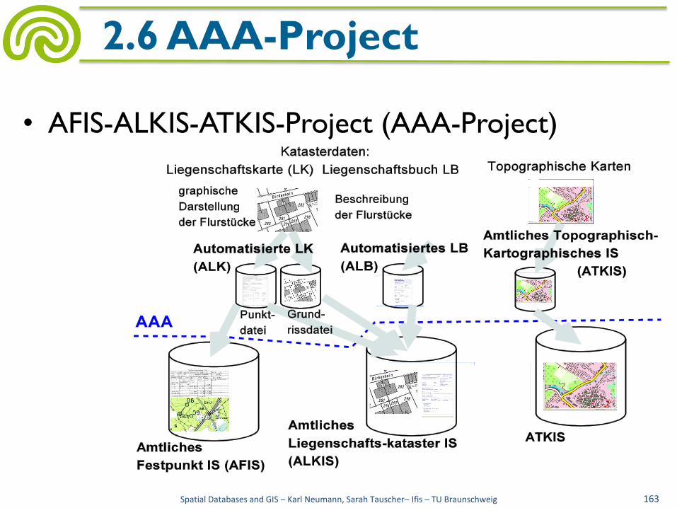
• AFIS-ALKIS-ATKIS-Project (AAA-Project)
Spatial Databases and GIS – Karl Neumann, Sarah Tauscher– Ifis – TU Braunschweig 163
2.6 AAA-Project
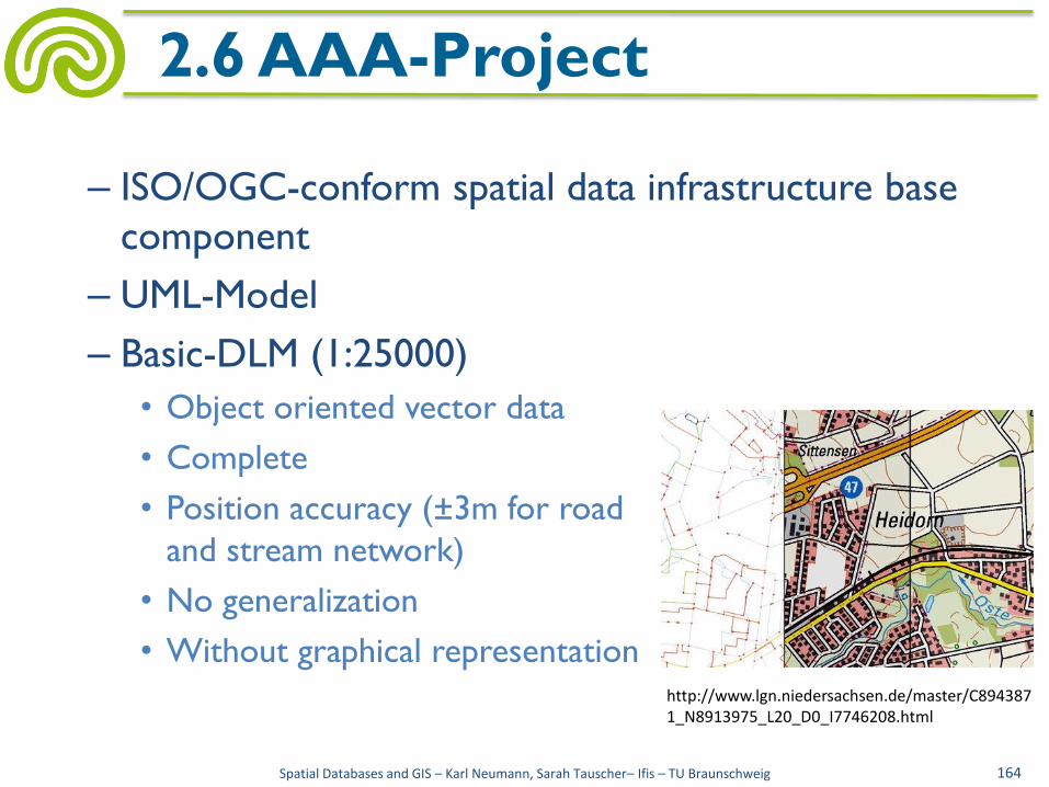
– ISO/OGC-conform spatial data infrastructure base
component
– UML-Model
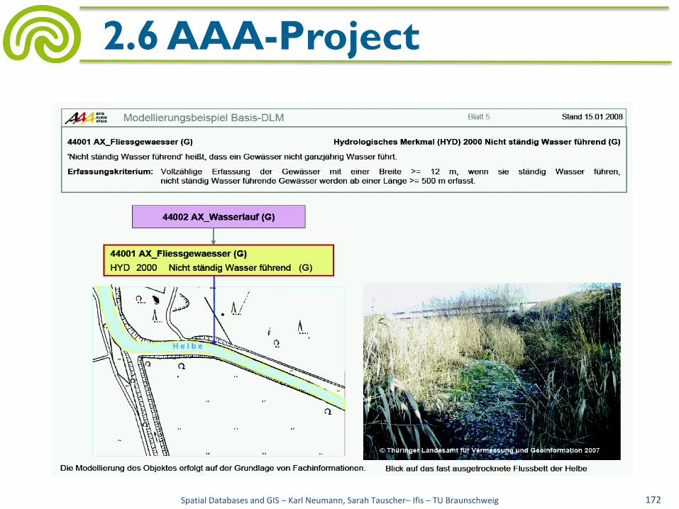
– Basic-DLM (1:25000)
• Object oriented vector data
• Complete
• Position accuracy (±3m for road
and stream network)
• No generalization
• Without graphical representation
Spatial Databases and GIS – Karl Neumann, Sarah Tauscher– Ifis – TU Braunschweig 164
2.6 AAA-Project
http://www.lgn.niedersachsen.de/master/C8943871_N8913975_L20_D0_I7746208.html
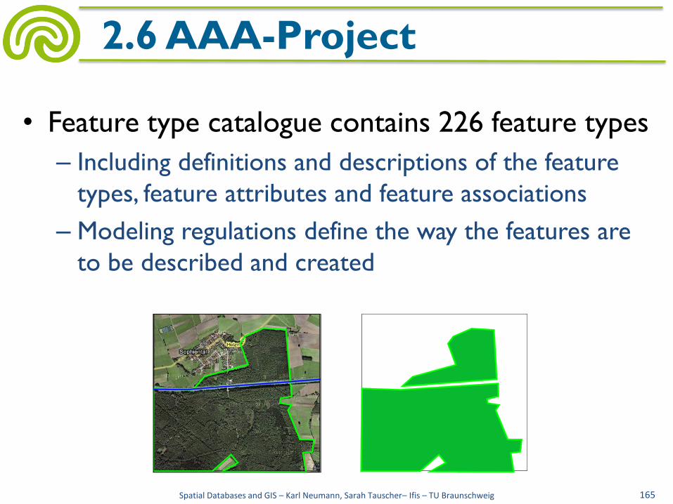
• Feature type catalogue contains 226 feature types
– Including definitions and descriptions of the feature
types, feature attributes and feature associations
– Modeling regulations define the way the features are
to be described and created
Spatial Databases and GIS – Karl Neumann, Sarah Tauscher– Ifis – TU Braunschweig 165
2.6 AAA-Project
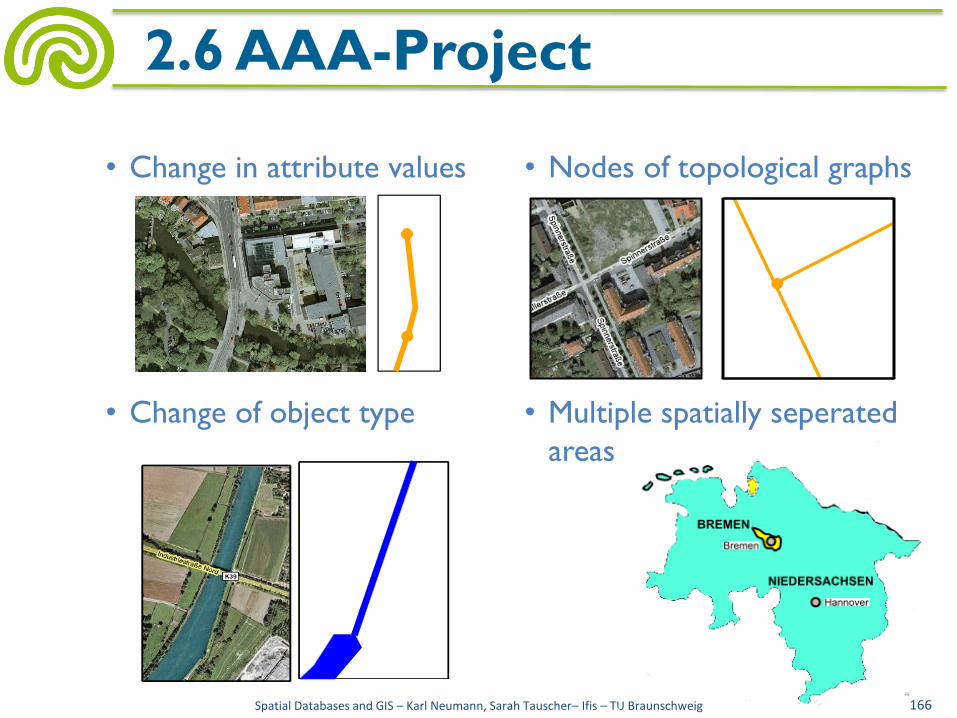
• Nodes of topological graphs
• Multiple spatially seperated
areas
• Change in attribute values
• Change of object type
Spatial Databases and GIS – Karl Neumann, Sarah Tauscher– Ifis – TU Braunschweig 166
2.6 AAA-Project
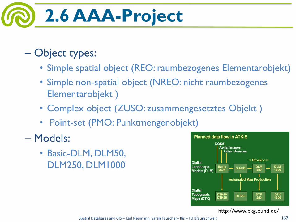
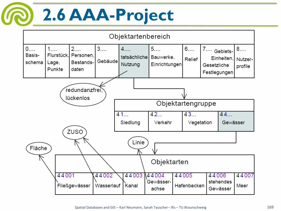
– Object types:
• Simple spatial object (REO: raumbezogenes Elementarobjekt)
• Simple non-spatial object (NREO: nicht raumbezogenes
Elementarobjekt )
• Complex object (ZUSO: zusammengesetztes Objekt )
• Point-set (PMO: Punktmengenobjekt)
– Models:
• Basic-DLM, DLM50,
DLM250, DLM1000
Spatial Databases and GIS – Karl Neumann, Sarah Tauscher– Ifis – TU Braunschweig 167
2.6 AAA-Project
http://www.bkg.bund.de/
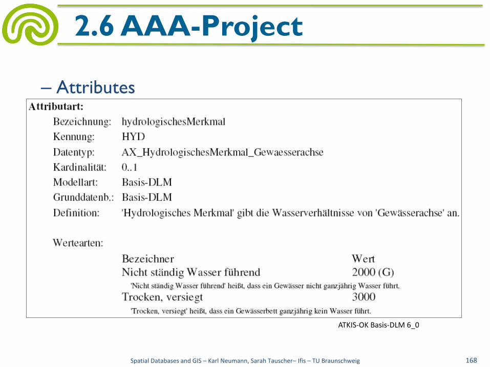
– Attributes
Spatial Databases and GIS – Karl Neumann, Sarah Tauscher– Ifis – TU Braunschweig 168
2.6 AAA-Project
ATKIS-OK Basis-DLM 6_0
Spatial Databases and GIS – Karl Neumann, Sarah Tauscher– Ifis – TU Braunschweig 169
2.6 AAA-Project
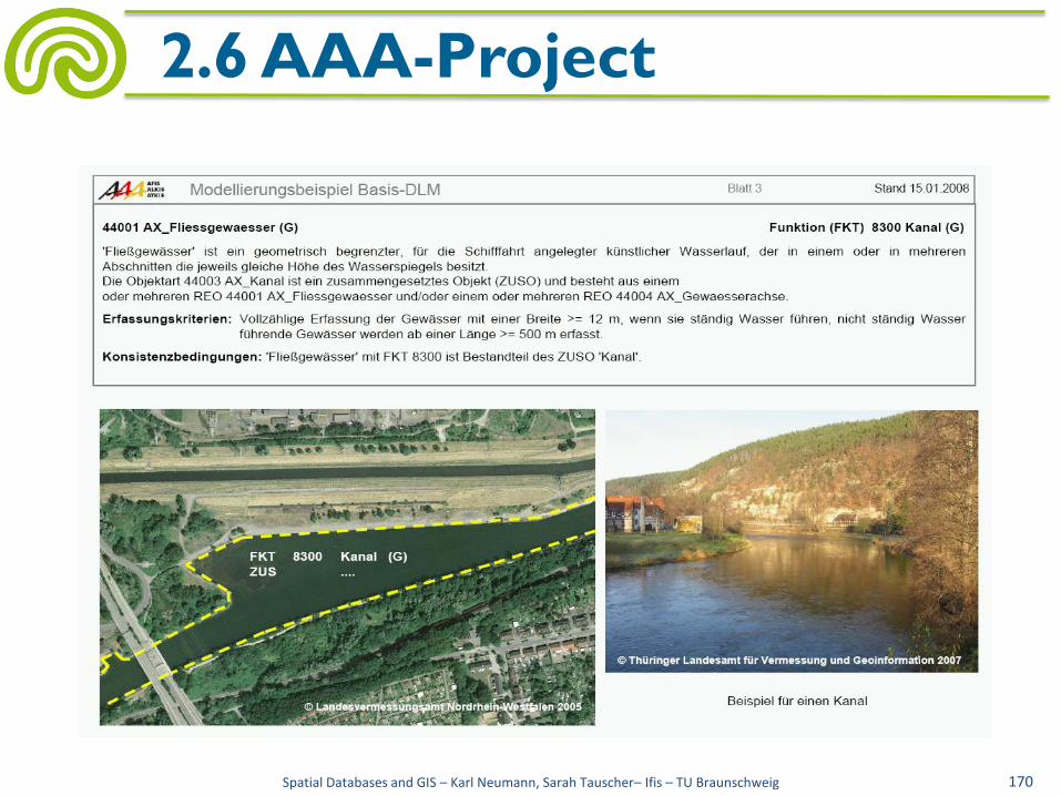
Spatial Databases and GIS – Karl Neumann, Sarah Tauscher– Ifis – TU Braunschweig 170
2.6 AAA-Project
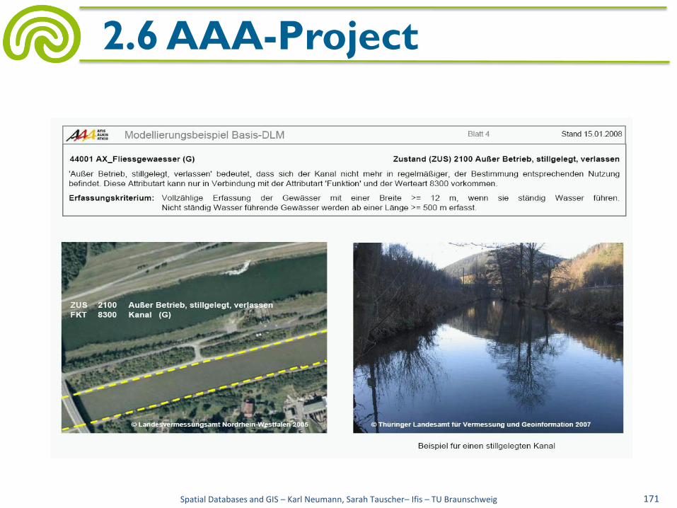
Spatial Databases and GIS – Karl Neumann, Sarah Tauscher– Ifis – TU Braunschweig 171
2.6 AAA-Project
Spatial Databases and GIS – Karl Neumann, Sarah Tauscher– Ifis – TU Braunschweig 172
2.6 AAA-Project
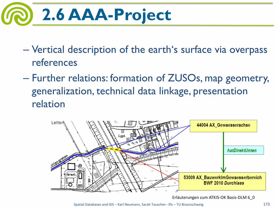
– Vertical description of the earth‘s surface via overpass
references
– Further relations: formation of ZUSOs, map geometry,
generalization, technical data linkage, presentation
relation
Spatial Databases and GIS – Karl Neumann, Sarah Tauscher– Ifis – TU Braunschweig 173
2.6 AAA-Project
Erläuterungen zum ATKIS-OK Basis-DLM 6_0
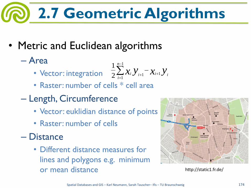
• Metric and Euclidean algorithms
– Area
• Vector: integration
• Raster: number of cells * cell area
– Length, Circumference
• Vector: euklidian distance of points
• Raster: number of cells
– Distance
• Different distance measures for
lines and polygons e.g. minimum
or mean distance
Spatial Databases and GIS – Karl Neumann, Sarah Tauscher– Ifis – TU Braunschweig 174
2.7 Geometric Algorithms
yxyx iii
n
ii 11
1
12
1
http://static1.fr.de/
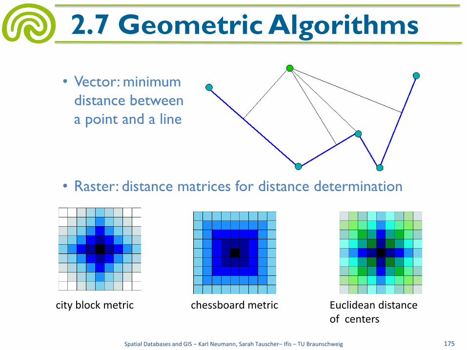
• Vector: minimum
distance between
a point and a line
• Raster: distance matrices for distance determination
Spatial Databases and GIS – Karl Neumann, Sarah Tauscher– Ifis – TU Braunschweig 175
2.7 Geometric Algorithms
city block metric chessboard metric Euclidean distance of centers

– Buffering
• Vector:
• Raster: building of a distance matrix, threshold
Spatial Databases and GIS – Karl Neumann, Sarah Tauscher– Ifis – TU Braunschweig 176
2.7 Geometric Algorithms
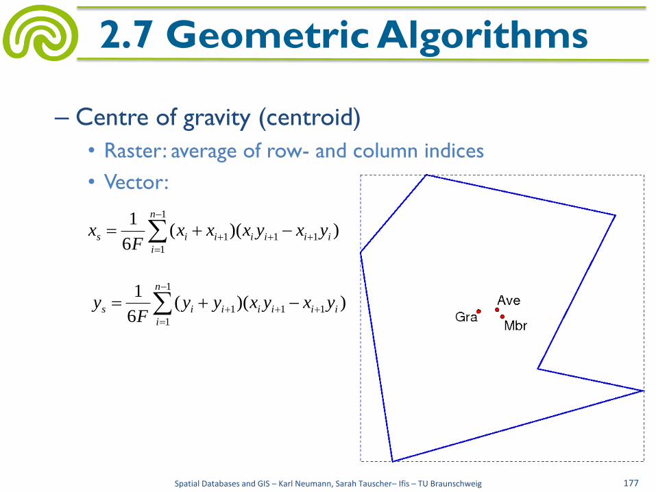
– Centre of gravity (centroid)
• Raster: average of row- and column indices
• Vector:
Spatial Databases and GIS – Karl Neumann, Sarah Tauscher– Ifis – TU Braunschweig 177
2.7 Geometric Algorithms
1
1
111 ))((6
1 n
i
iiiiiis yxyxxxF
x
1
1
111 ))((6
1 n
i
iiiiiis yxyxyyF
y
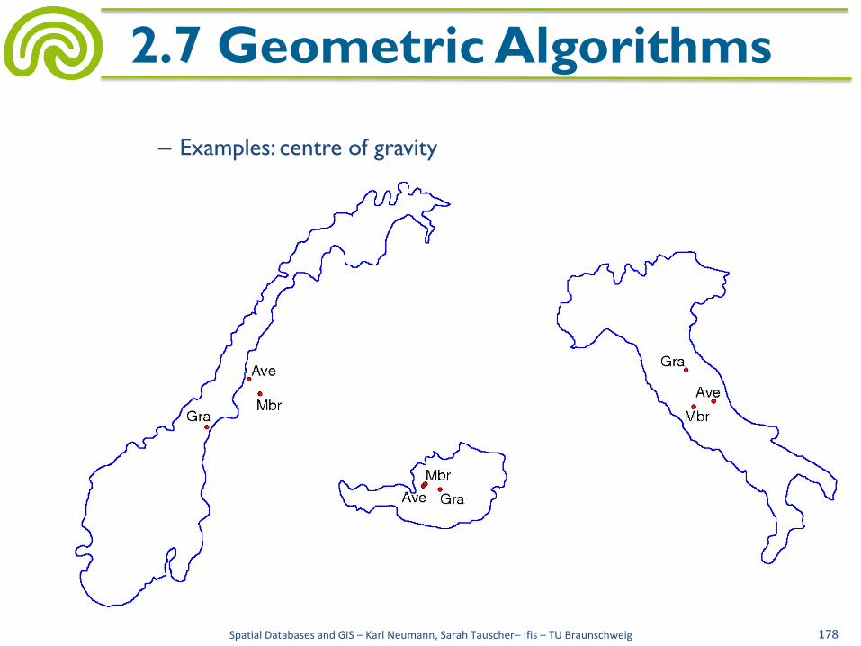
– Examples: centre of gravity
Spatial Databases and GIS – Karl Neumann, Sarah Tauscher– Ifis – TU Braunschweig 178
2.7 Geometric Algorithms
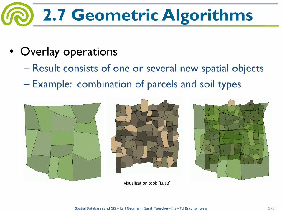
• Overlay operations
– Result consists of one or several new spatial objects
– Example: combination of parcels and soil types
Spatial Databases and GIS – Karl Neumann, Sarah Tauscher– Ifis – TU Braunschweig 179
2.7 Geometric Algorithms
visualization tool: [Lu13]
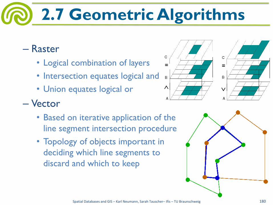
– Raster
• Logical combination of layers
• Intersection equates logical and
• Union equates logical or
– Vector
• Based on iterative application of the
line segment intersection procedure
• Topology of objects important in
deciding which line segments to
discard and which to keep
Spatial Databases and GIS – Karl Neumann, Sarah Tauscher– Ifis – TU Braunschweig 180
2.7 Geometric Algorithms
= =
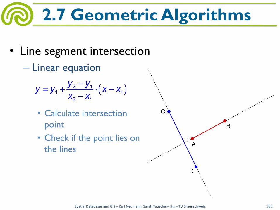
• Line segment intersection
– Linear equation
• Calculate intersection
point
• Check if the point lies on
the lines
Spatial Databases and GIS – Karl Neumann, Sarah Tauscher– Ifis – TU Braunschweig
2.7 Geometric Algorithms
181
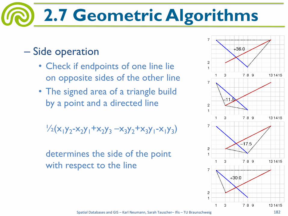
– Side operation
• Check if endpoints of one line lie
on opposite sides of the other line
• The signed area of a triangle build
by a point and a directed line
½(x1y2-x2y1+x2y3 –x3y2+x3y1-x1y3)
determines the side of the point
with respect to the line
Spatial Databases and GIS – Karl Neumann, Sarah Tauscher– Ifis – TU Braunschweig
2.7 Geometric Algorithms
182
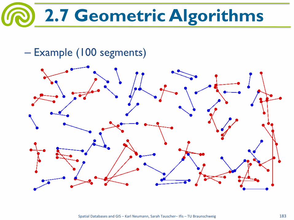
– Example (100 segments)
Spatial Databases and GIS – Karl Neumann, Sarah Tauscher– Ifis – TU Braunschweig
2.7 Geometric Algorithms
183
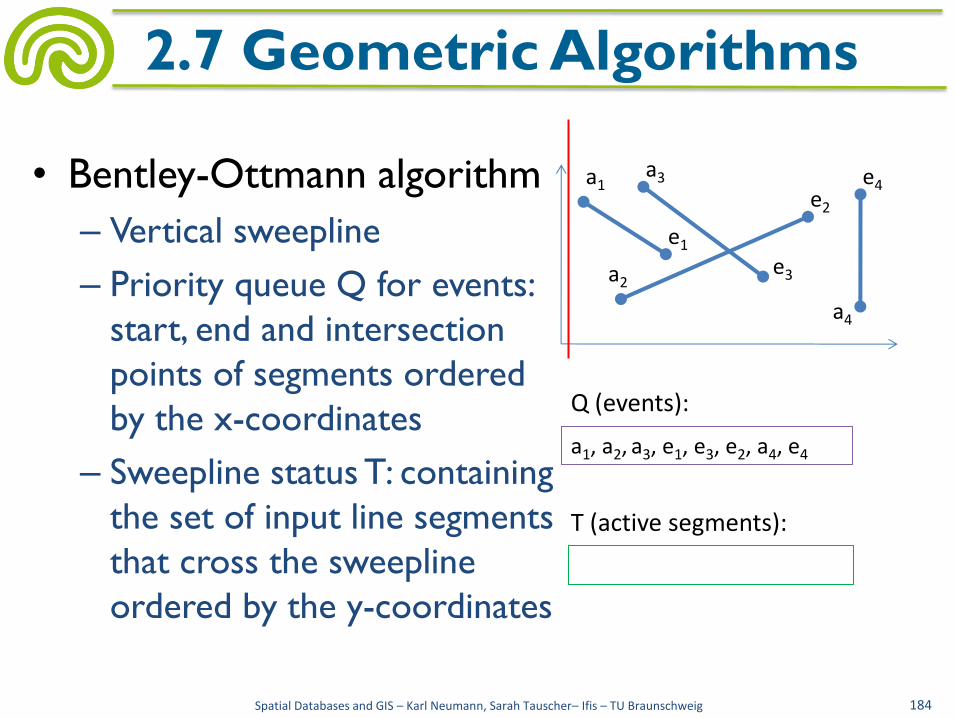
• Bentley-Ottmann algorithm
– Vertical sweepline
– Priority queue Q for events:
start, end and intersection
points of segments ordered
by the x-coordinates
– Sweepline status T: containing
the set of input line segments
that cross the sweepline
ordered by the y-coordinates
Spatial Databases and GIS – Karl Neumann, Sarah Tauscher– Ifis – TU Braunschweig 184
2.7 Geometric Algorithms
a1
a4
a3
a2
e1 e3
e2 e4
Q (events):
T (active segments):
a1, a2, a3, e1, e3, e2, a4, e4
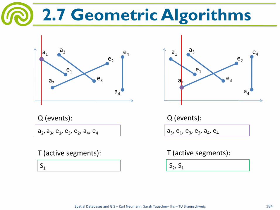
S2, S1
a3, e1, e3, e2, a4, e4 a2, a3, e1, e3, e2, a4, e4
Spatial Databases and GIS – Karl Neumann, Sarah Tauscher– Ifis – TU Braunschweig 184
2.7 Geometric Algorithms
a1
a4
a3
a2
e1 e3
e2 e4
Q (events):
T (active segments):
a1
a4
a3
a2
e1
e3
e2 e4
Q (events):
T (active segments):
S1
Spatial Databases and GIS – Karl Neumann, Sarah Tauscher– Ifis – TU Braunschweig 184
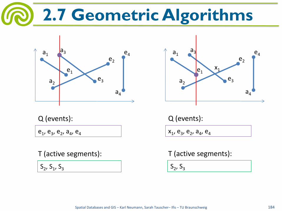
2.7 Geometric Algorithms
x1
a1
a4
a3
a2
e1 e3
e2 e4
Q (events):
T (active segments):
x1, e3, e2, a4, e4
S2, S3
a1
a4
a3
a2
e1
e3
e2 e4
Q (events):
T (active segments):
S2, S1, S3
e1, e3, e2, a4, e4
Spatial Databases and GIS – Karl Neumann, Sarah Tauscher– Ifis – TU Braunschweig 184
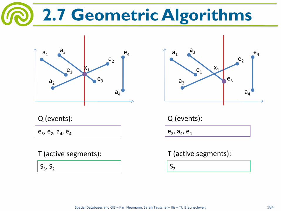
2.7 Geometric Algorithms
x1
a1
a4
a3
a2
e1 e3
e2 e4
Q (events):
T (active segments):
e2, a4, e4
S2
x1
a1
a4
a3
a2
e1
e3
e2 e4
Q (events):
T (active segments):
e3, e2, a4, e4
S3, S2
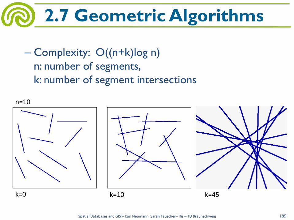
– Complexity: O((n+k)log n)
n: number of segments,
k: number of segment intersections
Spatial Databases and GIS – Karl Neumann, Sarah Tauscher– Ifis – TU Braunschweig 185
2.7 Geometric Algorithms
n=10
k=0 k=10 k=45
A
D C B
2
2 3
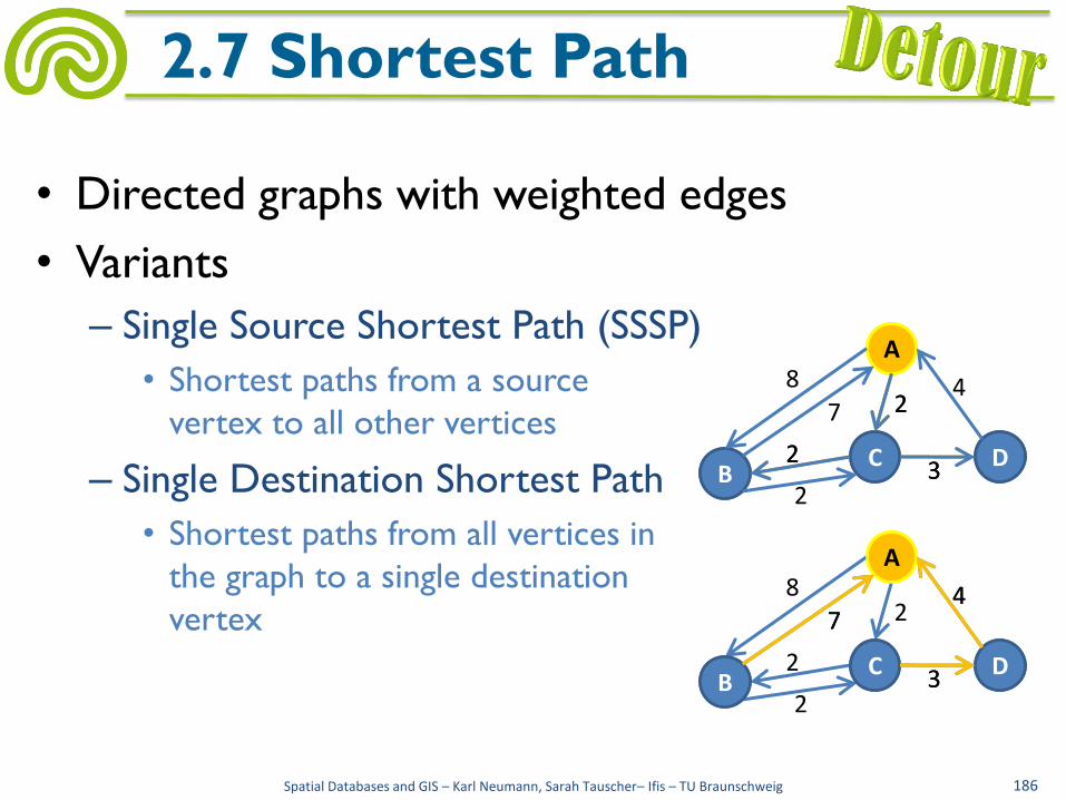
• Directed graphs with weighted edges
• Variants
– Single Source Shortest Path (SSSP)
• Shortest paths from a source
vertex to all other vertices
– Single Destination Shortest Path
• Shortest paths from all vertices in
the graph to a single destination
vertex
Spatial Databases and GIS – Karl Neumann, Sarah Tauscher– Ifis – TU Braunschweig 186
2.7 Shortest Path
A
D C B
7 8
2
2
2 3
4
A
D C B
7 8
2
2
2 3
4
A
D C B
7
3
4
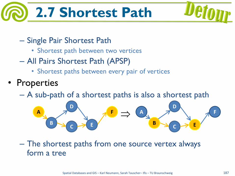
– Single Pair Shortest Path
• Shortest path between two vertices
– All Pairs Shortest Path (APSP)
• Shortest paths between every pair of vertices
• Properties
– A sub-path of a shortest paths is also a shortest path
– The shortest paths from one source vertex always form a tree
Spatial Databases and GIS – Karl Neumann, Sarah Tauscher– Ifis – TU Braunschweig 187
2.7 Shortest Path
A D
C B E
F A D
C B E
F
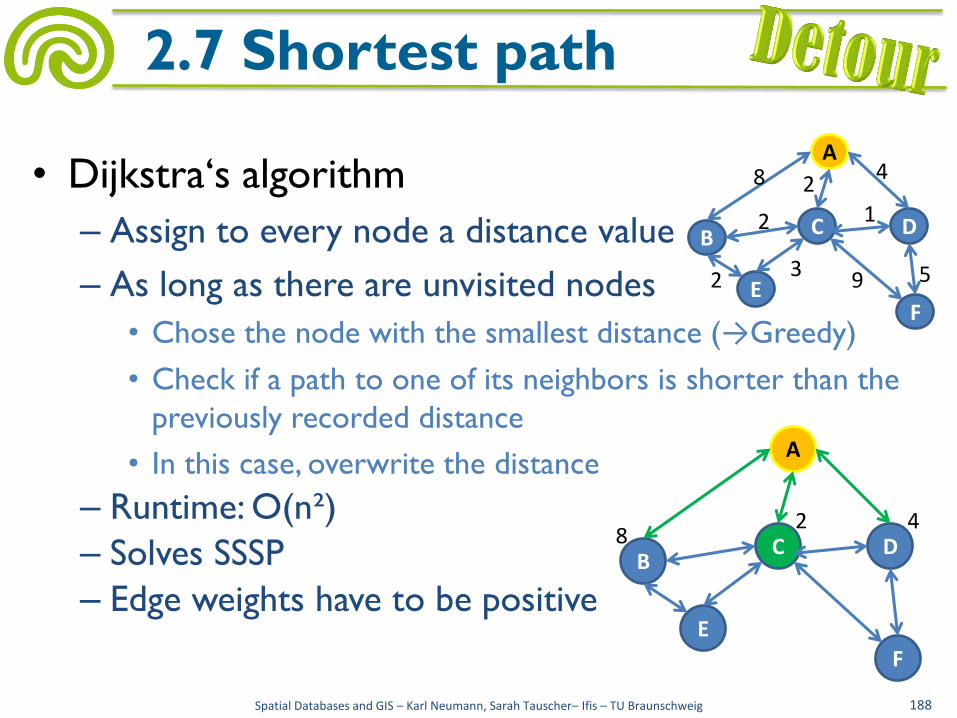
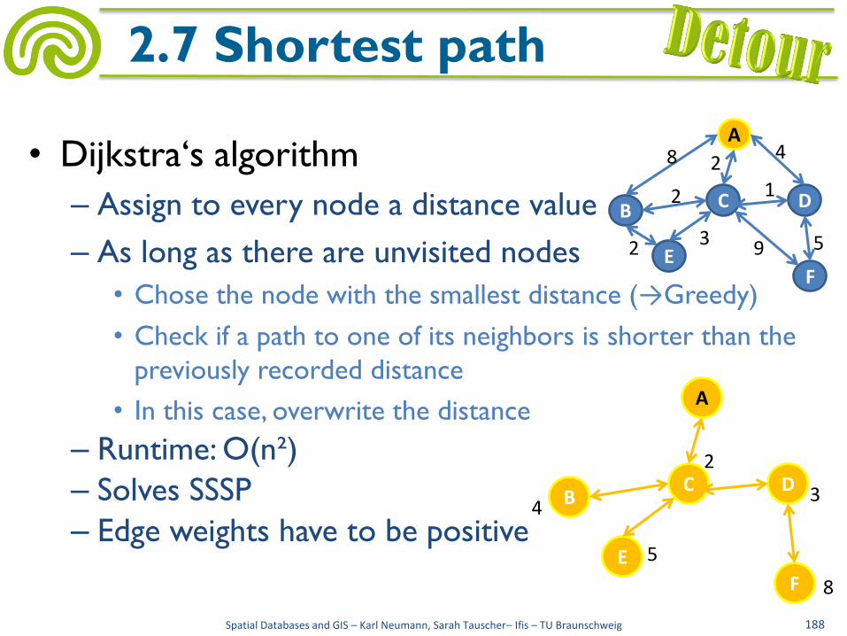
• Dijkstra‘s algorithm
– Assign to every node a distance value
– As long as there are unvisited nodes
• Chose the node with the smallest distance (→Greedy)
• Check if a path to one of its neighbors is shorter than the
previously recorded distance
• In this case, overwrite the distance
– Runtime: O(n²)
– Solves SSSP
– Edge weights have to be positive
Spatial Databases and GIS – Karl Neumann, Sarah Tauscher– Ifis – TU Braunschweig 188
2.7 Shortest path
A
F
E
D C B
8 2 4
A
F E
D C B 2
8 2 1
2 3 9 5
4
• Dijkstra‘s algorithm
– Assign to every node a distance value
– As long as there are unvisited nodes
• Chose the node with the smallest distance (→Greedy)
• Check if a path to one of its neighbors is shorter than the
previously recorded distance
• In this case, overwrite the distance
– Runtime: O(n²)
– Solves SSSP
– Edge weights have to be positive
Spatial Databases and GIS – Karl Neumann, Sarah Tauscher– Ifis – TU Braunschweig 188
2.7 Shortest path
A
F
E
D C B
2
3
11
5
A
F E
D C B 2
8 2 1
2 3 9 5
4
4
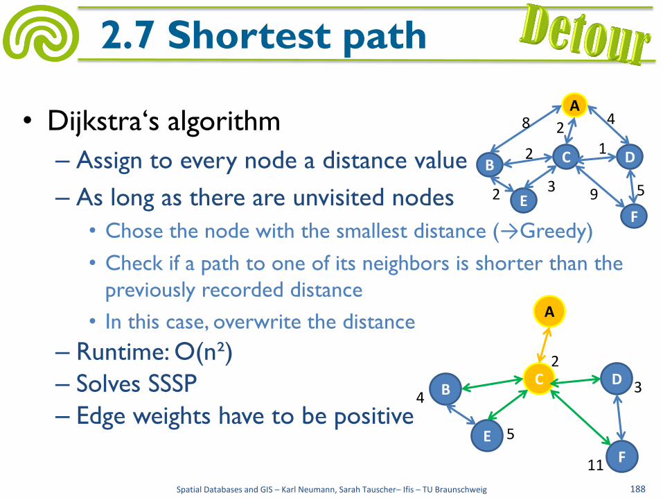
• Dijkstra‘s algorithm
– Assign to every node a distance value
– As long as there are unvisited nodes
• Chose the node with the smallest distance (→Greedy)
• Check if a path to one of its neighbors is shorter than the
previously recorded distance
• In this case, overwrite the distance
– Runtime: O(n²)
– Solves SSSP
– Edge weights have to be positive
Spatial Databases and GIS – Karl Neumann, Sarah Tauscher– Ifis – TU Braunschweig 188
2.7 Shortest path
A
F
E
D C B
2
3
8
5
A
F E
D C B 2
8 2 1
2 3 9 5
4
4
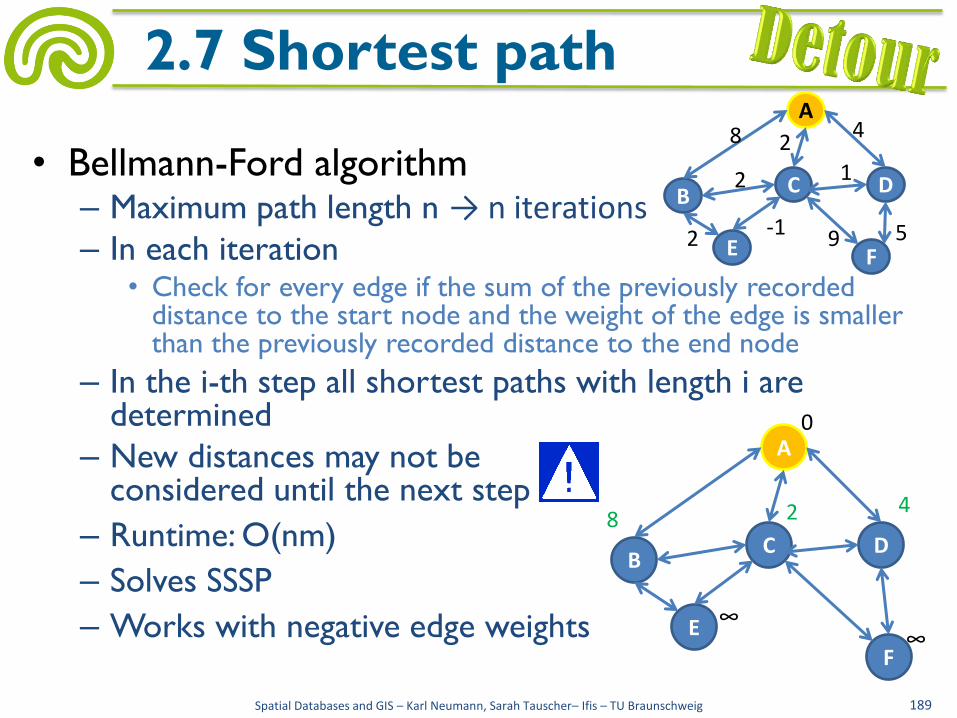
• Bellmann-Ford algorithm – Maximum path length n → n iterations – In each iteration
• Check for every edge if the sum of the previously recorded distance to the start node and the weight of the edge is smaller than the previously recorded distance to the end node
– In the i-th step all shortest paths with length i are determined
– New distances may not be considered until the next step
– Runtime: O(nm)
– Solves SSSP
– Works with negative edge weights
Spatial Databases and GIS – Karl Neumann, Sarah Tauscher– Ifis – TU Braunschweig 189
2.7 Shortest path
A
F
E
D C B
A
F E
D C B 2
8 2 1
2 -1 9 5
4
∞ ∞
0
8 2 4

• Bellmann-Ford algorithm – Maximum path length n → n iterations – In each iteration
• Check for every edge if the sum of the previously recorded distance to the start node and the weight of the edge is smaller than the previously recorded distance to the end node
– In the i-th step all shortest paths with length i are determined
– New distances may not be considered until the next step
– Runtime: O(nm)
– Solves SSSP
– Works with negative edge weights
Spatial Databases and GIS – Karl Neumann, Sarah Tauscher– Ifis – TU Braunschweig 189
2.7 Shortest path
A
F
E
D C B
A
F E
D C B 2
8 2 1
2 -1 9 5
4
0
2
4 3
1 9

• Bellmann-Ford algorithm – Maximum path length n → n iterations – In each iteration
• Check for every edge if the sum of the previously recorded distance to the start node and the weight of the edge is smaller than the previously recorded distance to the end node
– In the i-th step all shortest paths with length i are determined
– New distances may not be considered until the next step
– Runtime: O(nm)
– Solves SSSP
– Works with negative edge weights
Spatial Databases and GIS – Karl Neumann, Sarah Tauscher– Ifis – TU Braunschweig 189
2.7 Shortest path
A
F
E
D C B
A
F E
D C B 2
8 2 1
2 -1 9 5
4
0
2
8
3
1
3
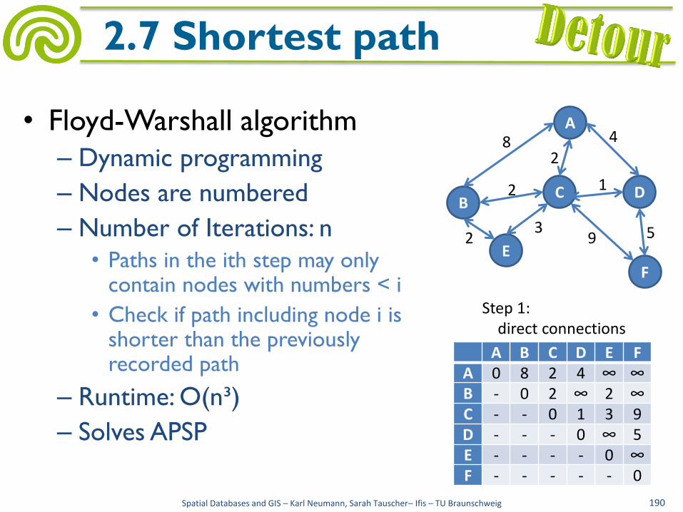
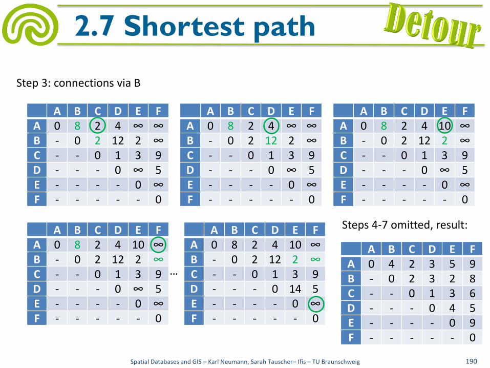
• Floyd-Warshall algorithm
– Dynamic programming
– Nodes are numbered
– Number of Iterations: n
• Paths in the ith step may only contain nodes with numbers < i
• Check if path including node i is shorter than the previously recorded path
– Runtime: O(n³)
– Solves APSP
Spatial Databases and GIS – Karl Neumann, Sarah Tauscher– Ifis – TU Braunschweig 190
2.7 Shortest path
A
F
E
D C B
2
8 2
1
2 3
9 5
4
Step 1: direct connections
A B C D E F A 0 8 2 4 ∞ ∞ B - 0 2 ∞ 2 ∞ C - - 0 1 3 9 D - - - 0 ∞ 5 E - - - - 0 ∞ F - - - - - 0
Spatial Databases and GIS – Karl Neumann, Sarah Tauscher– Ifis – TU Braunschweig 190
2.7 Shortest path
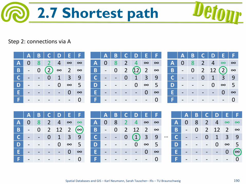
Step 2: connections via A
A B C D E F A 0 8 2 4 ∞ ∞ B - 0 2 ∞ 2 ∞ C - - 0 1 3 9 D - - - 0 ∞ 5 E - - - - 0 ∞ F - - - - - 0
A B C D E F A 0 8 2 4 ∞ ∞ B - 0 2 12 2 ∞ C - - 0 1 3 9 D - - - 0 ∞ 5 E - - - - 0 ∞ F - - - - - 0
A B C D E F A 0 8 2 4 ∞ ∞ B - 0 2 12 2 ∞ C - - 0 1 3 9 D - - - 0 ∞ 5 E - - - - 0 ∞ F - - - - - 0
A B C D E F A 0 8 2 4 ∞ ∞ B - 0 2 12 2 ∞ C - - 0 1 3 9 D - - - 0 ∞ 5 E - - - - 0 ∞ F - - - - - 0
A B C D E F A 0 8 2 4 ∞ ∞ B - 0 2 12 2 ∞ C - - 0 1 3 9 D - - - 0 ∞ 5 E - - - - 0 ∞ F - - - - - 0
A B C D E F A 0 8 2 4 ∞ ∞ B - 0 2 12 2 ∞ C - - 0 1 3 9 D - - - 0 ∞ 5 E - - - - 0 ∞ F - - - - - 0
…
Spatial Databases and GIS – Karl Neumann, Sarah Tauscher– Ifis – TU Braunschweig 190
2.7 Shortest path
Step 3: connections via B
A B C D E F A 0 8 2 4 ∞ ∞ B - 0 2 12 2 ∞ C - - 0 1 3 9 D - - - 0 ∞ 5 E - - - - 0 ∞ F - - - - - 0
A B C D E F A 0 8 2 4 ∞ ∞ B - 0 2 12 2 ∞ C - - 0 1 3 9 D - - - 0 ∞ 5 E - - - - 0 ∞ F - - - - - 0
A B C D E F A 0 8 2 4 10 ∞ B - 0 2 12 2 ∞ C - - 0 1 3 9 D - - - 0 ∞ 5 E - - - - 0 ∞ F - - - - - 0
A B C D E F A 0 8 2 4 10 ∞ B - 0 2 12 2 ∞ C - - 0 1 3 9 D - - - 0 ∞ 5 E - - - - 0 ∞ F - - - - - 0
A B C D E F A 0 8 2 4 10 ∞ B - 0 2 12 2 ∞ C - - 0 1 3 9 D - - - 0 14 5 E - - - - 0 ∞ F - - - - - 0
A B C D E F A 0 4 2 3 5 9 B - 0 2 3 2 8 C - - 0 1 3 6 D - - - 0 4 5 E - - - - 0 9 F - - - - - 0
Steps 4-7 omitted, result:
…
• Input: one or more fields
• Output: a resultant field
• Map algebra: system of possible operations on fields in a field-based model
• Five classes of operations (Tomlin 1990)
– Local
– Focal
– Zonal
– Global
– Incremental
Spatial Databases and GIS – Karl Neumann, Sarah Tauscher– Ifis – TU Braunschweig 191
2.7 Operations on Fields
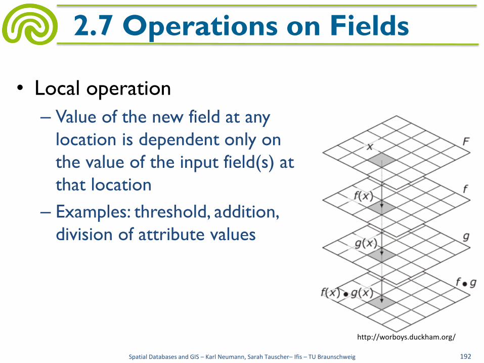
• Local operation
– Value of the new field at any
location is dependent only on
the value of the input field(s) at
that location
– Examples: threshold, addition,
division of attribute values
Spatial Databases and GIS – Karl Neumann, Sarah Tauscher– Ifis – TU Braunschweig 192
2.7 Operations on Fields
http://worboys.duckham.org/
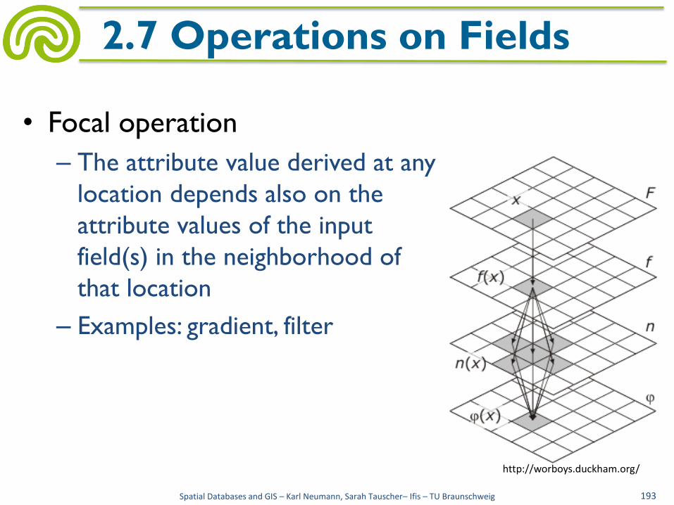
• Focal operation
– The attribute value derived at any
location depends also on the
attribute values of the input
field(s) in the neighborhood of
that location
– Examples: gradient, filter
Spatial Databases and GIS – Karl Neumann, Sarah Tauscher– Ifis – TU Braunschweig 193
2.7 Operations on Fields
http://worboys.duckham.org/
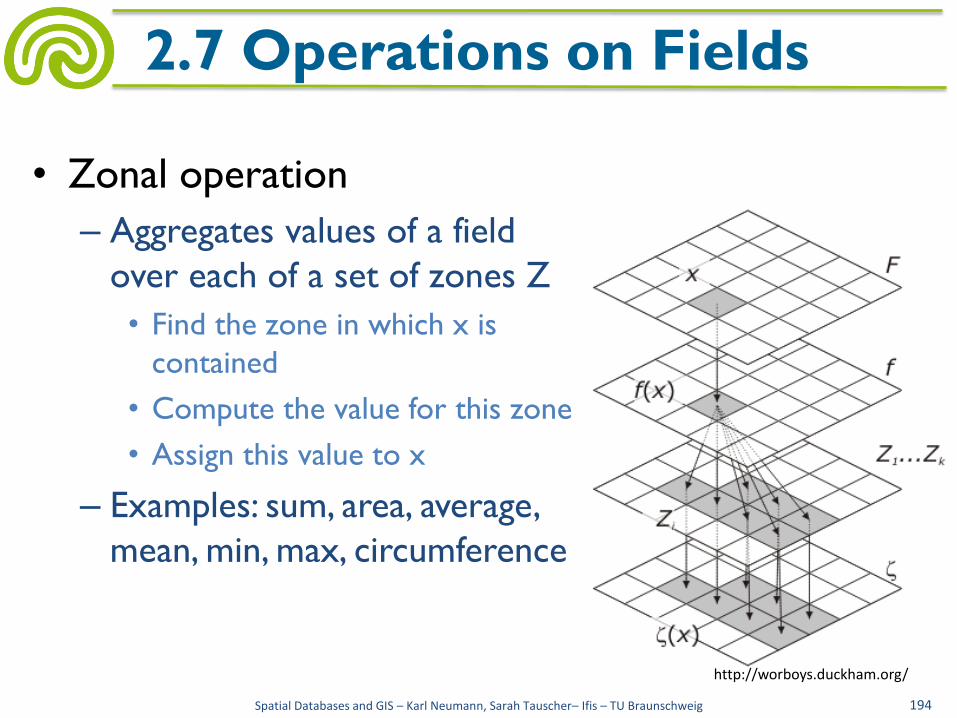
• Zonal operation
– Aggregates values of a field
over each of a set of zones Z
• Find the zone in which x is
contained
• Compute the value for this zone
• Assign this value to x
– Examples: sum, area, average,
mean, min, max, circumference
Spatial Databases and GIS – Karl Neumann, Sarah Tauscher– Ifis – TU Braunschweig 194
2.7 Operations on Fields
http://worboys.duckham.org/
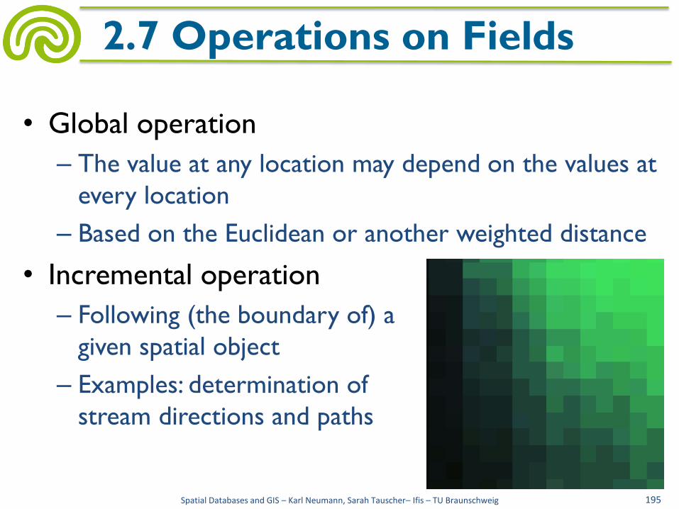
• Global operation
– The value at any location may depend on the values at
every location
– Based on the Euclidean or another weighted distance
• Incremental operation
– Following (the boundary of) a
given spatial object
– Examples: determination of
stream directions and paths
Spatial Databases and GIS – Karl Neumann, Sarah Tauscher– Ifis – TU Braunschweig 195
2.7 Operations on Fields
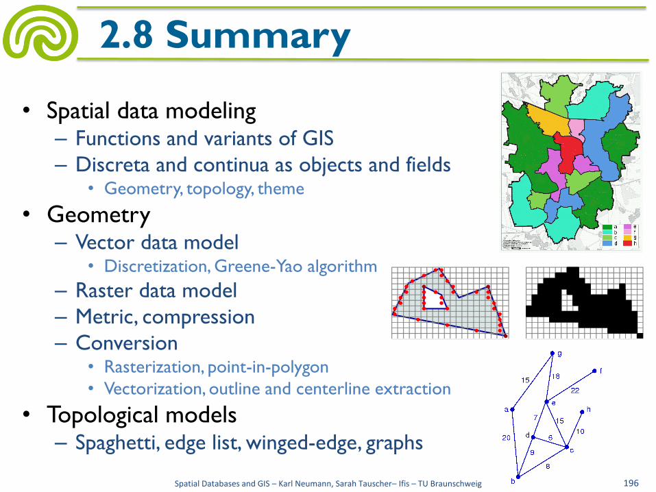
• Spatial data modeling – Functions and variants of GIS
– Discreta and continua as objects and fields • Geometry, topology, theme
• Geometry – Vector data model
• Discretization, Greene-Yao algorithm
– Raster data model
– Metric, compression
– Conversion • Rasterization, point-in-polygon
• Vectorization, outline and centerline extraction
• Topological models – Spaghetti, edge list, winged-edge, graphs
Spatial Databases and GIS – Karl Neumann, Sarah Tauscher– Ifis – TU Braunschweig 196
2.8 Summary
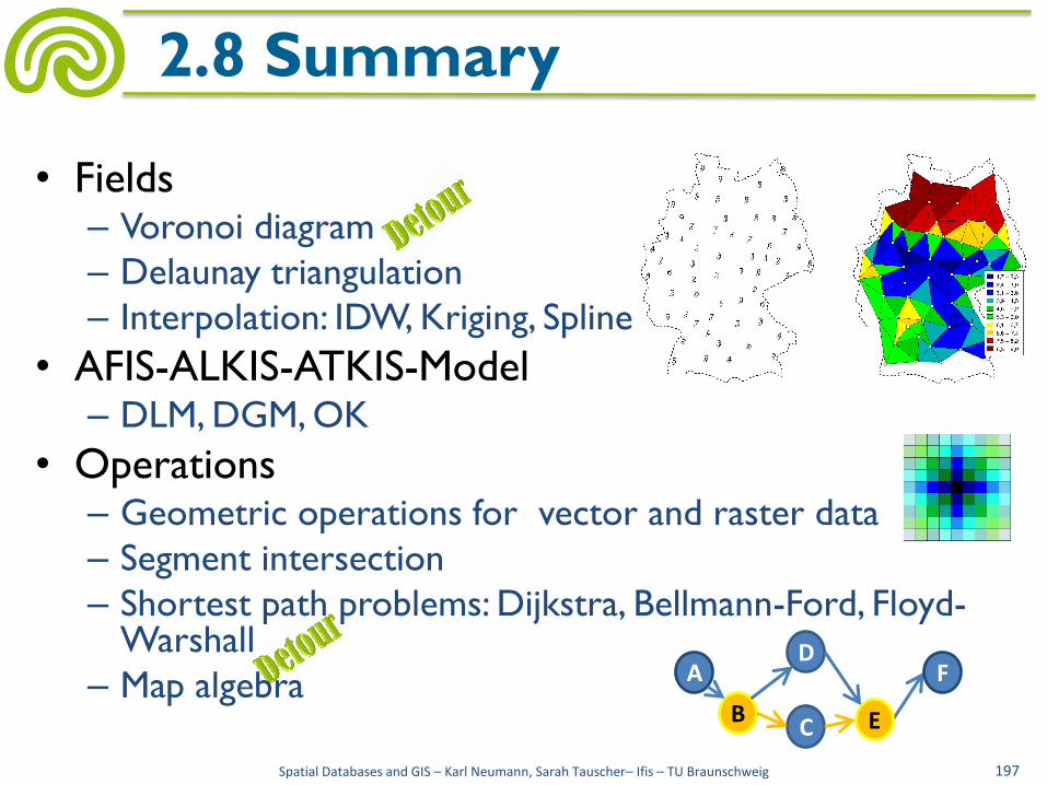
• Fields – Voronoi diagram
– Delaunay triangulation
– Interpolation: IDW, Kriging, Spline
• AFIS-ALKIS-ATKIS-Model – DLM, DGM, OK
• Operations – Geometric operations for vector and raster data
– Segment intersection
– Shortest path problems: Dijkstra, Bellmann-Ford, Floyd-Warshall
– Map algebra
Spatial Databases and GIS – Karl Neumann, Sarah Tauscher– Ifis – TU Braunschweig 197
2.8 Summary
A D
C B E
F
Spatial Databases and GIS – Karl Neumann, Sarah Tauscher– Ifis – TU Braunschweig 198
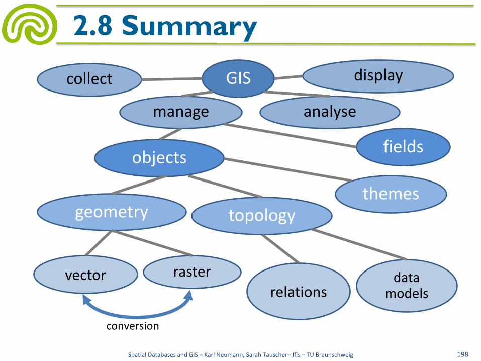
2.8 Summary
GIS
fields objects
themes topology geometry
data models relations
raster vector
collect
manage analyse
display
conversion
Spatial Databases and GIS – Karl Neumann, Sarah Tauscher– Ifis – TU Braunschweig 199
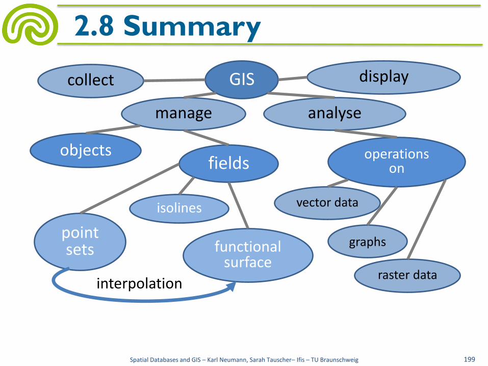
2.8 Summary
GIS
fields objects
functional surface
isolines
point sets
collect
manage analyse
display
interpolation
operations on
vector data
graphs
raster data