2018 Capital Market Assumptions - institutional.voya.com 3 Executive Summary Our 2018 Long Term Capital Market Assumptions details our Voya capital markets forecasts of asset class

INVESTMENT MANAGEMENT

Not FDIC Insured | May Lose Value | No Bank Guarantee

2018 Capital Market AssumptionsResearch Report byThe Multi-Asset Strategies and Solutions Team

Paul Zemsky, CFA Chief Investment Officer

Barbara Reinhard, CFA Head of Asset Allocation

Elias Belessakos, PhD Senior Quantitative Analyst

Timothy Kearney, PhD Asset Allocation Strategist

Jonathan Kaczka, CFA Asset Allocation Analyst

Daniel Wang Research Analyst

2

ForewordWhen financial market historians look back at 2017, the year probably will be highlighted for its tightly compressed levels of volatility. Another notable aspect of the year is that, heading into late December, there has not been a single month of negative returns for the S&P 500 index. It’s an impressive gain by almost any measure and relatively uncommon; the last time it happened was in 1995. Globally, equity market gains were strong. Average gains of more than 20% for developed markets were outshone only by the emerging markets, with average gains over 30%. Though such returns are striking by most measures, they probably would not make it into the chronicles of Martin Fridson’s 1998 book, It Was a Very Good Year: Extraordinary Moments in Stock Market History, a must read for anyone interested in financial market history. What we find most impressive about this year’s gains is that they are being notched in the eighth year of an expansion.

As we look forward to 2018, we think it useful not only to consider what the capital markets will deliver, but also what they have the potential to deliver. As we survey the landscape we are reminded that the starting point matters. Our work suggests that the robust returns which equities and bonds have produced over the past five years have extracted a certain amount of future return potential from our equilibrium assumptions. Our methodology assumes that markets will achieve equilibrium over the 10-year horizon. To a certain extent, returns that the S&P 500 index has delivered in recent years have borrowed from future potential gains.

As we have previously noted, among the unusual hallmarks of this expansion has been how well-anchored bond yields have stayed in the face of strongly rising equity markets. Lack of inflation too has been noticeable, wage and price pressures usually accompany aging growth cycles. A dearth of capital investment also has plagued this cycle. These issues, while not new, again confront investors as they think through portfolio positioning for the ninth year of this economic expansion. We have given these issues a great deal of research, which we share with our readers in the Macroeconomic section — with investment thought leadership on the business cycle and inflation.

We hope our readers find this content helpful as they navigate the year and next decade ahead. At Voya, we aspire to be America’s Retirement Company; to plan, invest and protect every step of the way. We thank you for your continued confidence in us.

Paul Zemsky, CFA Barbara Reinhard, CFA Chief Investment Officer Head, Asset Allocation Multi-Asset Strategies and Solutions Multi-Asset Strategies and Solutions

Table of Contents

Foreword 2

Executive Summary 3

Forecast Environment 3

Assumptions for the Target Date Glide Path 4

How Returns Are Forecast 6

Macroeconomic Considerations 10Tracking the Business Cycle 10

Inflation Trends to the Downside 16

Methodological Considerations 24Covariance and Correlation Matrices Methodology 24

Time Dependency of Asset Returns and Its Impact on Risk Estimation 26

Multi-Asset Strategies and Solutions Team 28

3

Executive SummaryOur 2018 Long Term Capital Market Assumptions details our Voya capital markets forecasts of asset class returns, standard deviation of returns and correlations over the 2018-2027 timeframe. These estimates are key inputs to our strategic asset allocation process for our multi-asset portfolios; they also provide a context for shorter-term economic and financial forecasting.

We continue to expect that the next 10-year period will be characterized by below-average historical returns, to varying degrees, across all asset classes. Our current forecast is for U.S. and international developed market equities to produce low, single-digit returns, which is lower than we forecast a year ago. Part of this is due to the unexpectedly strong performance by risk assets this year, which raised the bar for the coming 10 years. However, it is also a function of the current slow potential growth trajectory, influenced by the headwinds of slowing labor supply and an economy mired in a low-productivity regime.

Risk-adjusted returns for developed international market assets are in most cases lower than those for comparable U.S. assets. This partially reflects our expectation that the U.S. dollar is unlikely to depreciate meaningfully over the 10-year horizon due to tighter monetary policies and the potential for higher relative growth. Returns for emerging market equities are above U.S. large-cap returns on both an absolute basis as well as a Sharpe ratio basis given the positive overall growth trends and potential for re-rating.

Our bond return assumptions show that returns will generally be in the low single digits. Two exceptions to this trend are the emerging markets and leveraged loans. In the case of emerging markets, sustained growth would aid this high yielding sector. We expect leveraged loans to deliver as the Fed goes through a potentially long hiking cycle. We note that our projections do assume that both bond term premium moves and real rate premium moves will pressure bond prices lower.

Beyond our risk/return assumptions, this paper has two special sections: Macroeconomic Considerations and Methodological Considerations. The macroeconomic section features deep dives on two important questions: (1) where are we in the current business cycle? and (2) is there a dynamic in play which will keep inflation trending to the downside? The methodological section discusses our process of forecasting the covariance and correlations of returns, including the concept of turbulence. Turbulence bespeaks the fact that while 70% of the time markets exhibit “normal” behavior, market covariances reflect greater risk 30% of the time.

Forecast EnvironmentOur long-term capital market assumptions provide our estimates of expected returns, volatilities and correlations among major U.S. and global asset classes over a 10-year horizon. These estimates guide the strategic asset allocation for our multi-asset portfolios and provide a context for shorter-term economic and financial forecasting.

As has been the case for the past seven years, our forecast models an explicit process of convergence to a steady-state equilibrium for global economies and financial markets through 2018–2027. In our modeling process, we worked with Macroeconomic Advisers.

We believe that cyclical fluctuations are an inevitable aspect of market economies and therefore recognize that the steady-state equilibrium incorporated as the terminal point of our forecast is unlikely to be fully attained over any single 10-year period. Nonetheless, we believe that this is a useful construct for anchoring the forecast. As a result, the forecast does not assume a further recession or contraction over its 10-year horizon.

4

We make this explicit forecast in recognition of the ongoing effects of the 2007–09 financial crisis and recession, the European debt crisis and the fiscal and monetary policy responses to these events. Although the world economy is several years past its most acute point of crisis in 2008 and the U.S. economy has been recovering from the Great Recession for more than eight years, a number of economic and financial variables remain far from levels consistent with a steady state. In particular, short-term interest rates remain near zero in most developed economies, long-term interest rates have declined substantially, and government debt-to-GDP ratios remain elevated.

Still Low GrowthThe estimates for our U.S. economic and financial variables that underpin the analytics which formulate our expectations for asset class returns are shown in Figure 1. We forecast U.S. GDP growth to average 2.2%, a marginal 0.2% increase from our forecast last year. We believe the United States remains in a low growth environment, as the main sources of incremental growth would likely come from meaningful increases in the labor force growth or in productivity.

These two components imply potential GDP growth of only slightly above what we have experienced since the last recession. Given this backdrop our Federal Funds forecast has been downgraded to 2.7% from 3.1% last year and the 10-year U.S. Treasury yield forecast has declined to 3.6% from 4.1%. Figure 1 shows the 2027 values of our key macro assumptions from this forecast, which is consistent with our estimates of the longer-term steady state for key U.S. economic variables.

Figure 1. U.S. Economic and Financial Variables

2027 Forecast (%)GDP Growth 2.2Inflation (CPI-U) 2.2CPI excluding Food and Energy 2.3Fed Funds Rate 2.7Ten-Year Treasury Yield 3.6S&P 500 Earnings Growth 3.7Savings Rate 5.6Source: Voya Investment Management and Macroeconomic Advisers. Forecasts are subject to change.

Assumptions for the Target Date Glide PathWhile 10-year forecasts guide our strategic asset allocations, our long-run equilibrium return assumptions refer to horizons much longer than our ten-year forecasts, and are the underlying inputs into our glide path estimations. Typically, we assume the horizon for these forecasts is 40 years, at which point the economy is thought of as being in a steady state where GDP grows at its trend rate, inflation is at target, unemployment equals the non-accelerating inflation rate of unemployment, the real interest rate equals the natural rate of interest and all capital and goods markets are in equilibrium.

5

Our glide path model solves the portfolio choice problem over the life cycle, incorporating human capital in addition to financial capital. The crucial correlation between labor income and equities, which is low on average, provides the basis for the declining allocation to risky assets as a function of age. Early on, bond-like human capital is a large share of wealth and allows the individual to allocate a large share in the risky asset given the low relative riskiness of human capital. As investors age, and have fewer years of labor income ahead of them, financial capital becomes a greater share of their wealth. The optimal response is to reduce the allocation to the risky asset to compensate for the increase in riskiness of wealth. Thus, human capital is the driving force behind the glide path’s declining allocation to equities as a function of age.

These forecasts use a building block methodology. Starting with our expectations of real short-term yield and inflation, we generate a risk-free rate forecast and, from that, all equities and fixed income assets are derived by adding relevant risk premiums. The risk premium for U.S. equities is derived from the Gordon growth model as the sum of the dividend yield and the nominal earnings growth rate in excess of the risk-free rate. International equities include the addition of an international equity risk premium. Government bond return forecasts are the sum of the risk-free rate and an appropriate term premium. Corporate bond return forecasts further include the addition of a credit risk premium.

From a theoretical perspective, all risk premiums in long-run equilibrium are mean reverting since the economy has reached a steady state. Our econometric work confirms the stationarity of a number of risk premiums, which in turn justifies our assumption of constant average risk premiums, term premiums and credit spreads in the long-run equilibrium. Our equilibrium return forecasts are shown in Figure 2.

Figure 2. Long-Run Equilibrium Return Assumptions

Equilibrium Return (%)U.S. Inflation 2.0Real Risk-Free Rate 1.0U.S. Cash 3.0Aggregate Term Premium 0.9Aggregate Credit Premium 0.3U.S. Investment Grade (Aggregate) 4.210-Year Term Premium 1.210-Year U.S. Treasury 4.230-10 Year Term Premium 0.530-Year U.S. Treasury 4.7AA Corporate Credit Premium 1.2U.S. AA Corporate 5.4U.S. Equity Risk Premium 4.0S&P 500 7.0International Equity Premium 0.5MSCI ACWI 7.5Source: Voya Investment Management, data as of December 2016. Assumptions are subject to change.

6

How Returns Are ForecastWe derive asset class return forecasts from the blend of base case and alternative case economic scenarios. Together these capture the most important upside and downside risks the world economy and markets will face over the forecast horizon. The base case forecasts growth to average 2% through 2027 driven by continued below-trend productivity growth and subdued labor force growth. The alternative scenario assumes slightly faster productivity growth, modestly higher corporate profit share of income, higher dividend payout ratio and an assumption that the Fed lets the economy run a little hotter than in the base case. Given these assumptions, returns to risky assets are higher in the alternative scenario than in the base case.

We assign a probability of 65% to the base case and 35% to the alternative case. The higher probability for the base scenario reflects our view that recent trends toward an aging population, reduced labor force participation and more restrictive immigration could continue and result in a sustained, low U.S. growth rate.

For U.S. equities, we estimate earnings and dividends for the S&P 500 index using our blended macroeconomic assumptions. Earnings growth is constrained by the neoclassical assumption that profits as a share of GDP cannot increase without limit, but converge to a long-run equilibrium. We then use a dividend discount model to determine fair value for the index each year during the forecast period. Returns for other U.S. equity indices, including REITs, are constructed using a single index factor model in which beta sensitivities of each asset class with respect to the market portfolio are derived from our forward-looking covariance matrix estimation. For a detailed discussion on this, please refer to the covariance and correlation section. Each equity asset class return is the sum of the risk-free interest rate and a specific market-risk premium determined from our estimate of beta sensitivity and market risk premium forecasts.

For U.S. bonds, we use the blended scenario interest rate expectations to calculate expected returns for various durations. Bond expected returns are modeled as the sum of current yield and a capital gain (or loss) based on duration and expected change in yields. For non-U.S. bonds, the process is similar and includes an adjustment for expected currency movements. Return expectations for credit-related fixed income reflect yield spreads and expected default-and-recovery rates.

7

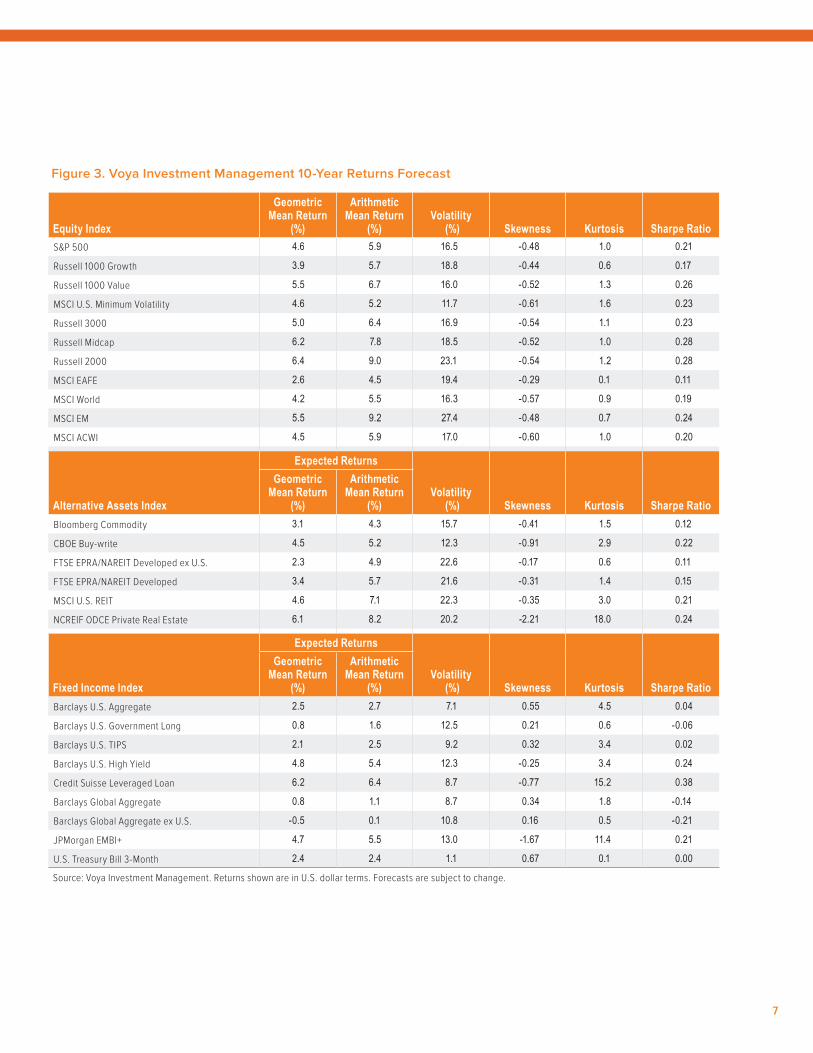
Figure 3. Voya Investment Management 10-Year Returns Forecast

Equity Index

Geometric Mean Return

(%)

Arithmetic Mean Return

(%)Volatility

(%) Skewness Kurtosis Sharpe RatioS&P 500 4.6 5.9 16.5 -0.48 1.0 0.21

Russell 1000 Growth 3.9 5.7 18.8 -0.44 0.6 0.17

Russell 1000 Value 5.5 6.7 16.0 -0.52 1.3 0.26

MSCI U.S. Minimum Volatility 4.6 5.2 11.7 -0.61 1.6 0.23

Russell 3000 5.0 6.4 16.9 -0.54 1.1 0.23

Russell Midcap 6.2 7.8 18.5 -0.52 1.0 0.28

Russell 2000 6.4 9.0 23.1 -0.54 1.2 0.28

MSCI EAFE 2.6 4.5 19.4 -0.29 0.1 0.11

MSCI World 4.2 5.5 16.3 -0.57 0.9 0.19

MSCI EM 5.5 9.2 27.4 -0.48 0.7 0.24

MSCI ACWI 4.5 5.9 17.0 -0.60 1.0 0.20

Expected Returns

Alternative Assets Index


(%)


(%)Volatility

(%) Skewness Kurtosis Sharpe RatioBloomberg Commodity 3.1 4.3 15.7 -0.41 1.5 0.12

CBOE Buy-write 4.5 5.2 12.3 -0.91 2.9 0.22

FTSE EPRA/NAREIT Developed ex U.S. 2.3 4.9 22.6 -0.17 0.6 0.11

FTSE EPRA/NAREIT Developed 3.4 5.7 21.6 -0.31 1.4 0.15

MSCI U.S. REIT 4.6 7.1 22.3 -0.35 3.0 0.21

NCREIF ODCE Private Real Estate 6.1 8.2 20.2 -2.21 18.0 0.24

Expected Returns

Fixed Income Index


(%)


(%)Volatility

(%) Skewness Kurtosis Sharpe RatioBarclays U.S. Aggregate 2.5 2.7 7.1 0.55 4.5 0.04

Barclays U.S. Government Long 0.8 1.6 12.5 0.21 0.6 -0.06

Barclays U.S. TIPS 2.1 2.5 9.2 0.32 3.4 0.02

Barclays U.S. High Yield 4.8 5.4 12.3 -0.25 3.4 0.24

Credit Suisse Leveraged Loan 6.2 6.4 8.7 -0.77 15.2 0.38

Barclays Global Aggregate 0.8 1.1 8.7 0.34 1.8 -0.14

Barclays Global Aggregate ex U.S. -0.5 0.1 10.8 0.16 0.5 -0.21

JPMorgan EMBI+ 4.7 5.5 13.0 -1.67 11.4 0.21

U.S. Treasury Bill 3-Month 2.4 2.4 1.1 0.67 0.1 0.00

Source: Voya Investment Management. Returns shown are in U.S. dollar terms. Forecasts are subject to change.

8

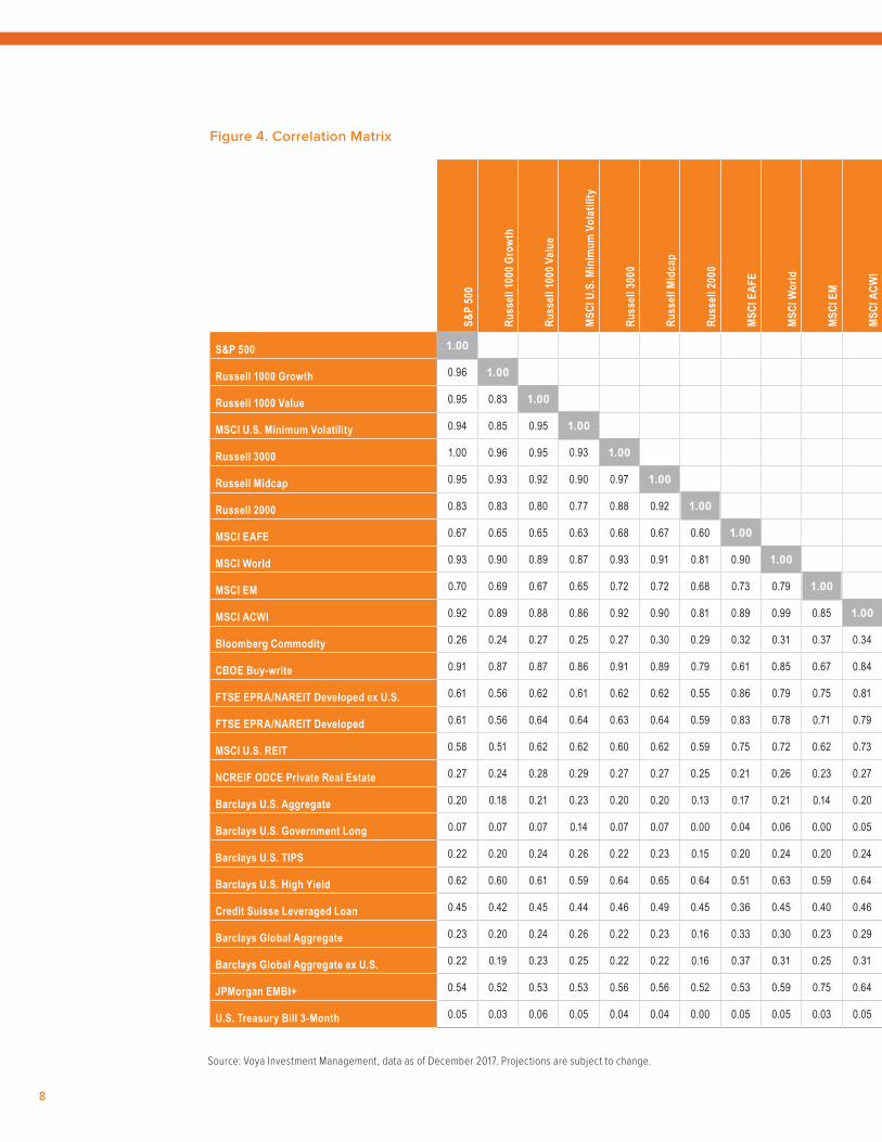
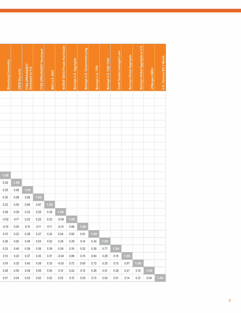
Figure 4. Correlation Matrix

S&P

500

Russ

ell 1

000 G

rowt

h

Russ

ell 1

000 V

alue

MSC

I U.S

. Min

imum

Vol

atili

ty

Russ

ell 3

000

Russ

ell M

idca

p

Russ

ell 2

000

MSC

I EAF

E

MSC

I Wor

ld

MSC

I EM

MSC

I ACW

I

Bloo

mbe

rg C

omm

odity

CBOE

Buy

-writ

e

FTSE

EPR

A/NA

REIT

De

velo

ped

ex U

.S.

FTSE

EPR

A/NA

REIT

Dev

elop

ed

MSC

I U.S

. REI

T

NCRE

IF O

DCE

Priv

ate R

eal E

stat

e

Barc

lays

U.S

. Agg

rega

te

Barc

lays

U.S

. Gov

ernm

ent L

ong

Barc

lays

U.S

. TIP

S

Barc

lays

U.S

. Hig

h Yi

eld

Cred

it Su

isse

Lev

erag

ed L

oan

Barc

lays

Glo

bal A

ggre

gate

Barc

lays

Glo

bal A

ggre

gate

ex U

.S.

JPM

orga

n EM

BI+

U.S.

Trea

sury

Bill

3-M

onth

S&P 500 1.00

Russell 1000 Growth 0.96 1.00

Russell 1000 Value 0.95 0.83 1.00

MSCI U.S. Minimum Volatility 0.94 0.85 0.95 1.00

Russell 3000 1.00 0.96 0.95 0.93 1.00

Russell Midcap 0.95 0.93 0.92 0.90 0.97 1.00

Russell 2000 0.83 0.83 0.80 0.77 0.88 0.92 1.00

MSCI EAFE 0.67 0.65 0.65 0.63 0.68 0.67 0.60 1.00

MSCI World 0.93 0.90 0.89 0.87 0.93 0.91 0.81 0.90 1.00

MSCI EM 0.70 0.69 0.67 0.65 0.72 0.72 0.68 0.73 0.79 1.00

MSCI ACWI 0.92 0.89 0.88 0.86 0.92 0.90 0.81 0.89 0.99 0.85 1.00

Bloomberg Commodity 0.26 0.24 0.27 0.25 0.27 0.30 0.29 0.32 0.31 0.37 0.34 1.00

CBOE Buy-write 0.91 0.87 0.87 0.86 0.91 0.89 0.79 0.61 0.85 0.67 0.84 0.29 1.00

FTSE EPRA/NAREIT Developed ex U.S. 0.61 0.56 0.62 0.61 0.62 0.62 0.55 0.86 0.79 0.75 0.81 0.35 0.56 1.00

FTSE EPRA/NAREIT Developed 0.61 0.56 0.64 0.64 0.63 0.64 0.59 0.83 0.78 0.71 0.79 0.30 0.58 0.96 1.00

MSCI U.S. REIT 0.58 0.51 0.62 0.62 0.60 0.62 0.59 0.75 0.72 0.62 0.73 0.23 0.55 0.85 0.97 1.00

NCREIF ODCE Private Real Estate 0.27 0.24 0.28 0.29 0.27 0.27 0.25 0.21 0.26 0.23 0.27 0.28 0.29 0.22 0.25 0.26 1.00

Barclays U.S. Aggregate 0.20 0.18 0.21 0.23 0.20 0.20 0.13 0.17 0.21 0.14 0.20 -0.02 0.17 0.22 0.22 0.20 -0.06 1.00

Barclays U.S. Government Long 0.07 0.07 0.07 0.14 0.07 0.07 0.00 0.04 0.06 0.00 0.05 -0.10 0.05 0.10 0.11 0.11 -0.14 0.89 1.00

Barclays U.S. TIPS 0.22 0.20 0.24 0.26 0.22 0.23 0.15 0.20 0.24 0.20 0.24 0.10 0.22 0.28 0.27 0.24 0.04 0.93 0.81 1.00

Barclays U.S. High Yield 0.62 0.60 0.61 0.59 0.64 0.65 0.64 0.51 0.63 0.59 0.64 0.26 0.62 0.49 0.53 0.52 0.29 0.29 0.14 0.34 1.00

Credit Suisse Leveraged Loan 0.45 0.42 0.45 0.44 0.46 0.49 0.45 0.36 0.45 0.40 0.46 0.23 0.45 0.36 0.39 0.39 0.39 0.19 0.02 0.26 0.77 1.00

Barclays Global Aggregate 0.23 0.20 0.24 0.26 0.22 0.23 0.16 0.33 0.30 0.23 0.29 0.13 0.20 0.37 0.35 0.31 -0.04 0.86 0.74 0.84 0.28 0.16 1.00

Barclays Global Aggregate ex U.S. 0.22 0.19 0.23 0.25 0.22 0.22 0.16 0.37 0.31 0.25 0.31 0.18 0.20 0.40 0.38 0.33 -0.03 0.72 0.60 0.72 0.25 0.13 0.97 1.00

JPMorgan EMBI+ 0.54 0.52 0.53 0.53 0.56 0.56 0.52 0.53 0.59 0.75 0.64 0.26 0.55 0.59 0.59 0.54 0.15 0.22 0.15 0.26 0.51 0.28 0.21 0.19 1.00

U.S. Treasury Bill 3-Month 0.05 0.03 0.06 0.05 0.04 0.04 0.00 0.05 0.05 0.03 0.05 0.01 0.04 0.03 0.02 0.02 0.03 0.15 0.05 0.13 0.00 0.01 0.14 0.12 0.04 1.00

Source: Voya Investment Management, data as of December 2017. Projections are subject to change.

9

Figure 4. Correlation Matrix

S&P

500

Russ

ell 1

000 G

rowt

h

Russ

ell 1

000 V

alue

MSC

I U.S

. Min

imum

Vol

atili

ty

Russ

ell 3

000

Russ

ell M

idca

p

Russ

ell 2

000

MSC

I EAF

E

MSC

I Wor

ld

MSC

I EM

MSC

I ACW

I

Bloo

mbe

rg C

omm

odity

CBOE

Buy

-writ

e

FTSE

EPR

A/NA

REIT

De

velo

ped

ex U

.S.

FTSE

EPR

A/NA

REIT

Dev

elop

ed

MSC

I U.S

. REI

T

NCRE

IF O

DCE

Priv

ate R

eal E

stat

e

Barc

lays

U.S

. Agg

rega

te

Barc

lays

U.S

. Gov

ernm

ent L

ong

Barc

lays

U.S

. TIP

S

Barc

lays

U.S

. Hig

h Yi

eld

Cred

it Su

isse

Lev

erag

ed L

oan

Barc

lays

Glo

bal A

ggre

gate

Barc

lays

Glo

bal A

ggre

gate

ex U

.S.

JPM

orga

n EM

BI+

U.S.

Trea

sury

Bill

3-M

onth

S&P 500 1.00

Russell 1000 Growth 0.96 1.00

Russell 1000 Value 0.95 0.83 1.00

MSCI U.S. Minimum Volatility 0.94 0.85 0.95 1.00

Russell 3000 1.00 0.96 0.95 0.93 1.00

Russell Midcap 0.95 0.93 0.92 0.90 0.97 1.00

Russell 2000 0.83 0.83 0.80 0.77 0.88 0.92 1.00

MSCI EAFE 0.67 0.65 0.65 0.63 0.68 0.67 0.60 1.00

MSCI World 0.93 0.90 0.89 0.87 0.93 0.91 0.81 0.90 1.00

MSCI EM 0.70 0.69 0.67 0.65 0.72 0.72 0.68 0.73 0.79 1.00

MSCI ACWI 0.92 0.89 0.88 0.86 0.92 0.90 0.81 0.89 0.99 0.85 1.00

Bloomberg Commodity 0.26 0.24 0.27 0.25 0.27 0.30 0.29 0.32 0.31 0.37 0.34 1.00

CBOE Buy-write 0.91 0.87 0.87 0.86 0.91 0.89 0.79 0.61 0.85 0.67 0.84 0.29 1.00

FTSE EPRA/NAREIT Developed ex U.S. 0.61 0.56 0.62 0.61 0.62 0.62 0.55 0.86 0.79 0.75 0.81 0.35 0.56 1.00

FTSE EPRA/NAREIT Developed 0.61 0.56 0.64 0.64 0.63 0.64 0.59 0.83 0.78 0.71 0.79 0.30 0.58 0.96 1.00

MSCI U.S. REIT 0.58 0.51 0.62 0.62 0.60 0.62 0.59 0.75 0.72 0.62 0.73 0.23 0.55 0.85 0.97 1.00

NCREIF ODCE Private Real Estate 0.27 0.24 0.28 0.29 0.27 0.27 0.25 0.21 0.26 0.23 0.27 0.28 0.29 0.22 0.25 0.26 1.00

Barclays U.S. Aggregate 0.20 0.18 0.21 0.23 0.20 0.20 0.13 0.17 0.21 0.14 0.20 -0.02 0.17 0.22 0.22 0.20 -0.06 1.00

Barclays U.S. Government Long 0.07 0.07 0.07 0.14 0.07 0.07 0.00 0.04 0.06 0.00 0.05 -0.10 0.05 0.10 0.11 0.11 -0.14 0.89 1.00

Barclays U.S. TIPS 0.22 0.20 0.24 0.26 0.22 0.23 0.15 0.20 0.24 0.20 0.24 0.10 0.22 0.28 0.27 0.24 0.04 0.93 0.81 1.00

Barclays U.S. High Yield 0.62 0.60 0.61 0.59 0.64 0.65 0.64 0.51 0.63 0.59 0.64 0.26 0.62 0.49 0.53 0.52 0.29 0.29 0.14 0.34 1.00

Credit Suisse Leveraged Loan 0.45 0.42 0.45 0.44 0.46 0.49 0.45 0.36 0.45 0.40 0.46 0.23 0.45 0.36 0.39 0.39 0.39 0.19 0.02 0.26 0.77 1.00

Barclays Global Aggregate 0.23 0.20 0.24 0.26 0.22 0.23 0.16 0.33 0.30 0.23 0.29 0.13 0.20 0.37 0.35 0.31 -0.04 0.86 0.74 0.84 0.28 0.16 1.00

Barclays Global Aggregate ex U.S. 0.22 0.19 0.23 0.25 0.22 0.22 0.16 0.37 0.31 0.25 0.31 0.18 0.20 0.40 0.38 0.33 -0.03 0.72 0.60 0.72 0.25 0.13 0.97 1.00

JPMorgan EMBI+ 0.54 0.52 0.53 0.53 0.56 0.56 0.52 0.53 0.59 0.75 0.64 0.26 0.55 0.59 0.59 0.54 0.15 0.22 0.15 0.26 0.51 0.28 0.21 0.19 1.00

U.S. Treasury Bill 3-Month 0.05 0.03 0.06 0.05 0.04 0.04 0.00 0.05 0.05 0.03 0.05 0.01 0.04 0.03 0.02 0.02 0.03 0.15 0.05 0.13 0.00 0.01 0.14 0.12 0.04 1.00

10

Macroeconomic Considerations

Tracking the Business CycleThe current expansion has lasted for more than 100 months as of this writing, and its long duration is creating concerns about the risk of an imminent recession. According to the National Bureau of Economic Research (NBER) there have been 11 business cycles from 1945 to 2009, with the average cycle lasting 69 months. The average expansion has lasted about 58 months with the average recession lasting about 11.

This historical data show that expansions do not exhibit what is called “duration dependence,” that is, there is no empirical relationship between the duration of an expansion and the likelihood of entering a downturn. By contrast, recessions have shown duration dependence, as do whole cycles.1 We have calculated the unconditional probability of being in a recession at any point over the coming 12 months. Assuming expansions end with a constant probability and without any other predictive variables we find:

■ A 19% unconditional probability of recession over any coming 12-month period

■ About a 50% recession probability over any 40-month period

■ An 18% unconditional probability of an expansion as long as the current one

The current expansion is not of an unlikely duration, being only a little longer than the average 92 months of the last three expansions.

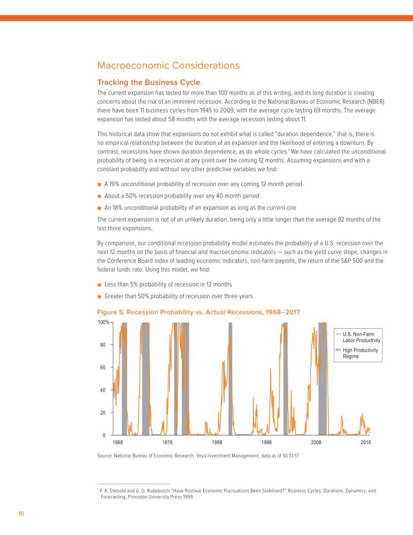
By comparison, our conditional recession probability model estimates the probability of a U.S. recession over the next 12 months on the basis of financial and macroeconomic indicators — such as the yield curve slope, changes in the Conference Board index of leading economic indicators, non-farm payrolls, the return of the S&P 500 and the federal funds rate. Using this model, we find:

■ Less than 5% probability of recession in 12 months

■ Greater than 50% probability of recession over three years

Figure 5. Recession Probability vs. Actual Recessions, 1968–2017

01978 19981968 1988 2008 2016

20

60

High Productivity Regime

U.S. Non-Farm Labor Productivity

40

80

100%

Source: National Bureau of Economic Research, Voya Investment Management, data as of 10/31/17.

1 F. X. Diebold and G. D. Rudebusch “Have Postwar Economic Fluctuations Been Stabilized?” Business Cycles: Durations, Dynamics, and Forecasting, Princeton University Press 1999.

11

Business cycles have moderated in the postwar period as the volatility of real output around trend has declined. That is, while complete business cycle durations have not changed, expansions have become longer while contractions have become shorter. In fact, the average duration of postwar expansions is double that of prewar expansions, with the average postwar contraction duration half that of prewar contractions.2 Some of the reasons for the longer expansions are structural:3

■ The decline in share of manufacturing and agriculture sectors relative to less volatile services sectors. Services now represent 77% of the value-added to U.S. GDP

■ About 69% of full- and part-time employment is concentrated in the private service sector. This figure rises to 85% with government jobs included

■ The broader availability of consumer credit has reduced consumer liquidity constraints and allows for consumption smoothing over business cycles. That is, there has been less direct dependence on current disposable income, which has led to a less volatile consumption pattern

■ Government spending has increased its share of GDP, with a more persistent spending pattern than private sector spending

■ Better monetary policy in recent decades has helped reduce cyclical fluctuations

Although every business cycle is different in that there is little evidence of periodicity4 or regularity in timing of the cycles, they all share the characteristics of co-movement of macroeconomic series and persistence. The co-movement characteristic is thought to be due to common, economy-wide shocks or underlying factors. There exist a number coincident economic activity indicators based on the idea of common factors extracted via principal components analysis.

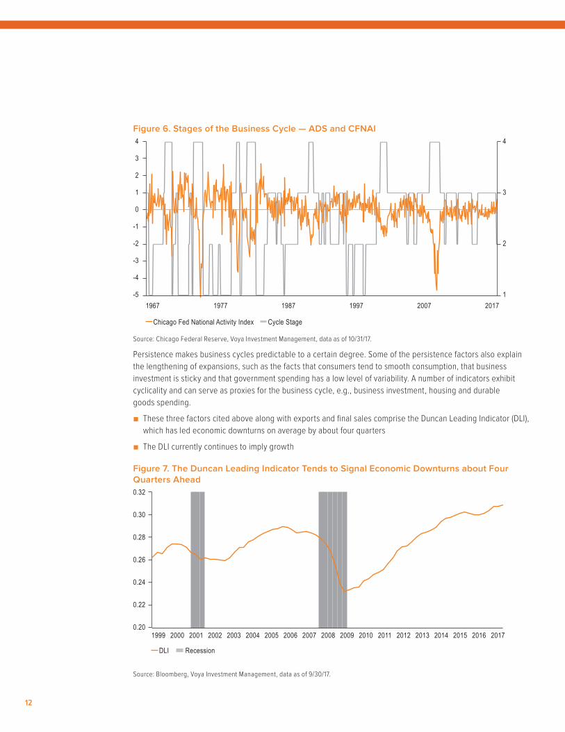
Two such indicators are the Chicago Fed National Activity Index (CFNAI) based on 85 individual indicators and the Aruoba-Diebold-Scotti (ADS) activity index based on six individual indicators of different frequencies. We use both of these indicators in our model of the stage of the business cycle. Our model exploits both co-movement and persistence via a Markov regime switching model, and attempts to identify the stage of the business cycle and predict turning points in economic activity.

■ This analysis identifies the current stage as mid-cycle with an expected duration of 11 months and a standard deviation of 8 months, but as mentioned earlier expansions do not show duration dependence

2 F. X. Diebold and G. D. Rudebusch “Shorter Recessions and Longer Expansions,” Business Cycles: Durations, Dynamics, and Forecasting, Princeton University Press 1999.

3 J. Bradford DeLong and L. H. Summers, “The Changing Cyclical Variability of Economic Activity in the United States,” The National Bureau of Economic Research, NBER Working Paper No. 1459, November 1986.

4 V. Zarnowitz, Business Cycles: Theory, History, Indicators and Forecasting (The University of Chicago Press, 1992), pp. 251–264.

12

Figure 6. Stages of the Business Cycle — ADS and CFNAI

Source: Chicago Federal Reserve, Voya Investment Management, data as of 10/31/17.

Persistence makes business cycles predictable to a certain degree. Some of the persistence factors also explain the lengthening of expansions, such as the facts that consumers tend to smooth consumption, that business investment is sticky and that government spending has a low level of variability. A number of indicators exhibit cyclicality and can serve as proxies for the business cycle, e.g., business investment, housing and durable goods spending.

■ These three factors cited above along with exports and final sales comprise the Duncan Leading Indicator (DLI), which has led economic downturns on average by about four quarters

■ The DLI currently continues to imply growth

Figure 7. The Duncan Leading Indicator Tends to Signal Economic Downturns about Four Quarters Ahead

Source: Bloomberg, Voya Investment Management, data as of 9/30/17.

1977 19971967 1987 2007 2017

Cycle StageChicago Fed National Activity Index

-5

-4

-3

-2

-1

0

1

2

3

4

1

2

3

4

1999 2016 2017

RecessionDLI

0.20

0.22

0.24

0.26

0.28

0.30

0.32

2015201420132012201120102009200820072006200520042003200220012000

13

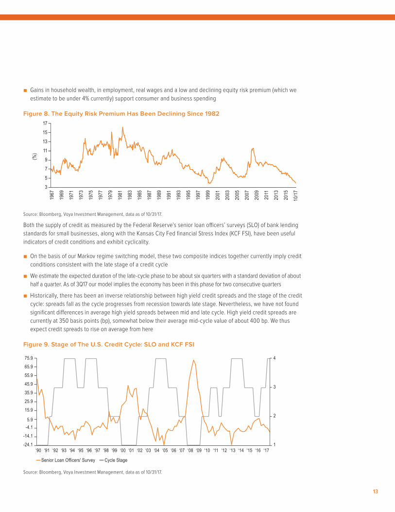
■ Gains in household wealth, in employment, real wages and a low and declining equity risk premium (which we estimate to be under 4% currently) support consumer and business spending

Figure 8. The Equity Risk Premium Has Been Declining Since 1982


Both the supply of credit as measured by the Federal Reserve’s senior loan officers’ surveys (SLO) of bank lending standards for small businesses, along with the Kansas City Fed financial Stress Index (KCF FSI), have been useful indicators of credit conditions and exhibit cyclicality.

■ On the basis of our Markov regime switching model, these two composite indices together currently imply credit conditions consistent with the late stage of a credit cycle

■ We estimate the expected duration of the late-cycle phase to be about six quarters with a standard deviation of about half a quarter. As of 3Q17 our model implies the economy has been in this phase for two consecutive quarters

■ Historically, there has been an inverse relationship between high yield credit spreads and the stage of the credit cycle: spreads fall as the cycle progresses from recession towards late stage. Nevertheless, we have not found significant differences in average high yield spreads between mid and late cycle. High yield credit spreads are currently at 350 basis points (bp), somewhat below their average mid-cycle value of about 400 bp. We thus expect credit spreads to rise on average from here

Figure 9. Stage of The U.S. Credit Cycle: SLO and KCF FSI


9/30/20176/30/2017

12/31/2016

12/31/201512/31/201412/31/2013

12/31/2012

12/31/201112/31/201012/31/200912/31/2008

12/31/2007

12/31/200612/31/200512/31/200412/31/200312/31/200212/31/200112/31/200012/31/199912/31/199812/31/199712/31/199612/31/1995

12/31/1994

12/31/199312/31/199212/31/199112/31/199012/31/198912/31/198812/31/198712/31/198612/31/198512/31/1983

12/31/1982

12/31/198112/31/198012/31/197812/31/197712/31/1976

12/31/1975

12/31/197412/31/197212/31/1971

12/31/1970

12/31/196912/31/1968

1967

2014

2015

2013

2016

10/1

7

2012

2009

2011

2007

2008

2005

2006

2010

2002

2003

2000

2001

2004

1985

1985

1983

1984

1987

1980

1981

1982

1978

1979

1976

1977

1973

1975

1971

1972

1969

1970

1974

1968

1998

1999

1996

1997

1994

1995

1992

1993

1990

1991

1988

1989

(%)

3

5

7

9

11

13

15

17

Cycle StageSenior Loan Officers' Survey

1

2

3

4

-24.1

-14.1

-4.15.9

15.9

25.9

35.9

45.9

55.9

65.9

75.9

‘99 ‘16 ‘17‘15‘14‘13‘12‘11‘10‘09‘08‘07‘06‘05‘04‘03‘02‘01‘00‘98‘97‘96‘95‘94‘93‘92‘91‘90

14

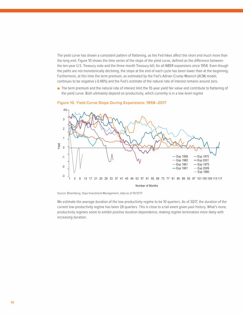
The yield curve has shown a consistent pattern of flattening, as the Fed hikes affect the short end much more than the long end. Figure 10 shows the time series of the slope of the yield curve, defined as the difference between the ten-year U.S. Treasury note and the three-month Treasury bill, for all NBER expansions since 1958. Even though the paths are not monotonically declining, the slope at the end of each cycle has been lower than at the beginning. Furthermore, at this time the term premium, as estimated by the Fed’s Adrian-Crump-Moench (ACM) model, continues to be negative (-0.48%) and the Fed’s estimate of the natural rate of interest remains around zero.

■ The term premium and the natural rate of interest limit the 10-year yield fair value and contribute to flattening of the yield curve. Both ultimately depend on productivity, which currently is in a low-level regime

Figure 10. Yield Curve Slope During Expansions: 1958–2017


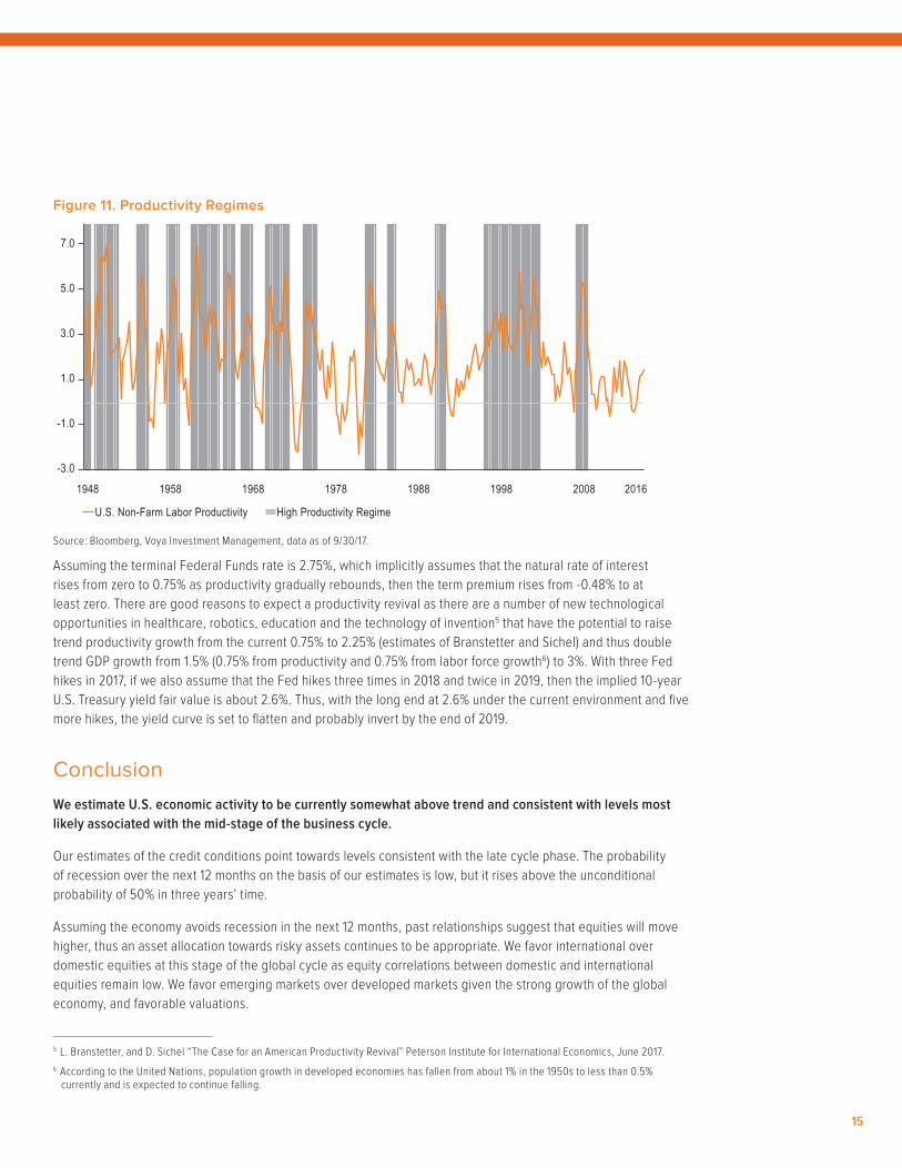
We estimate the average duration of the low-productivity regime to be 10 quarters. As of 3Q17, the duration of the current low-productivity regime has been 28 quarters. This is close to a tail event given past history. What’s more, productivity regimes seem to exhibit positive duration dependence, making regime termination more likely with increasing duration.

-3

-2

-1

0

1

2

3

4%

Exp 1958Exp 1982

69

Exp 1961Exp 1991

Exp 1970Exp 2001Exp 1975Exp 2009Exp 1980

65615753494541373329

Number of Months

Yield

25211713951 73 979389858177 101 113109105 117

15

Figure 11. Productivity Regimes


Assuming the terminal Federal Funds rate is 2.75%, which implicitly assumes that the natural rate of interest rises from zero to 0.75% as productivity gradually rebounds, then the term premium rises from -0.48% to at least zero. There are good reasons to expect a productivity revival as there are a number of new technological opportunities in healthcare, robotics, education and the technology of invention5 that have the potential to raise trend productivity growth from the current 0.75% to 2.25% (estimates of Branstetter and Sichel) and thus double trend GDP growth from 1.5% (0.75% from productivity and 0.75% from labor force growth6) to 3%. With three Fed hikes in 2017, if we also assume that the Fed hikes three times in 2018 and twice in 2019, then the implied 10-year U.S. Treasury yield fair value is about 2.6%. Thus, with the long end at 2.6% under the current environment and five more hikes, the yield curve is set to flatten and probably invert by the end of 2019.

ConclusionWe estimate U.S. economic activity to be currently somewhat above trend and consistent with levels most likely associated with the mid-stage of the business cycle.

Our estimates of the credit conditions point towards levels consistent with the late cycle phase. The probability of recession over the next 12 months on the basis of our estimates is low, but it rises above the unconditional probability of 50% in three years’ time.

Assuming the economy avoids recession in the next 12 months, past relationships suggest that equities will move higher, thus an asset allocation towards risky assets continues to be appropriate. We favor international over domestic equities at this stage of the global cycle as equity correlations between domestic and international equities remain low. We favor emerging markets over developed markets given the strong growth of the global economy, and favorable valuations.

5 L. Branstetter, and D. Sichel “The Case for an American Productivity Revival” Peterson Institute for International Economics, June 2017.6 According to the United Nations, population growth in developed economies has fallen from about 1% in the 1950s to less than 0.5%

currently and is expected to continue falling.

1948 1958 1978 19981968 1988 2008 2016

High Productivity RegimeU.S. Non-Farm Labor Productivity

-3.0

-1.0

1.0

3.0

5.0

7.0

16

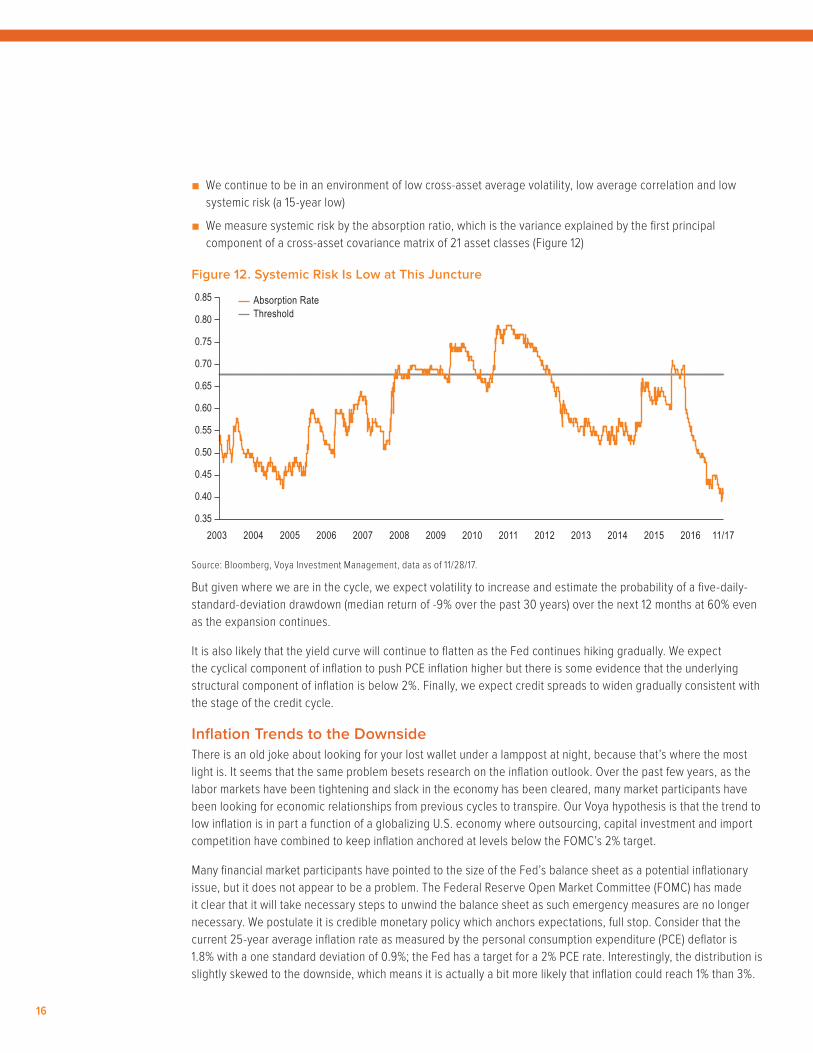
■ We continue to be in an environment of low cross-asset average volatility, low average correlation and low systemic risk (a 15-year low)

■ We measure systemic risk by the absorption ratio, which is the variance explained by the first principal component of a cross-asset covariance matrix of 21 asset classes (Figure 12)

Figure 12. Systemic Risk Is Low at This Juncture


But given where we are in the cycle, we expect volatility to increase and estimate the probability of a five-daily-standard-deviation drawdown (median return of -9% over the past 30 years) over the next 12 months at 60% even as the expansion continues.

It is also likely that the yield curve will continue to flatten as the Fed continues hiking gradually. We expect the cyclical component of inflation to push PCE inflation higher but there is some evidence that the underlying structural component of inflation is below 2%. Finally, we expect credit spreads to widen gradually consistent with the stage of the credit cycle.

Inflation Trends to the DownsideThere is an old joke about looking for your lost wallet under a lamppost at night, because that’s where the most light is. It seems that the same problem besets research on the inflation outlook. Over the past few years, as the labor markets have been tightening and slack in the economy has been cleared, many market participants have been looking for economic relationships from previous cycles to transpire. Our Voya hypothesis is that the trend to low inflation is in part a function of a globalizing U.S. economy where outsourcing, capital investment and import competition have combined to keep inflation anchored at levels below the FOMC’s 2% target.

Many financial market participants have pointed to the size of the Fed’s balance sheet as a potential inflationary issue, but it does not appear to be a problem. The Federal Reserve Open Market Committee (FOMC) has made it clear that it will take necessary steps to unwind the balance sheet as such emergency measures are no longer necessary. We postulate it is credible monetary policy which anchors expectations, full stop. Consider that the current 25-year average inflation rate as measured by the personal consumption expenditure (PCE) deflator is 1.8% with a one standard deviation of 0.9%; the Fed has a target for a 2% PCE rate. Interestingly, the distribution is slightly skewed to the downside, which means it is actually a bit more likely that inflation could reach 1% than 3%.

2003 2004 2006 20082005 2007 2009 20112010 2012 2013 2014 2015 11/172016

Absorption RateThreshold

0.50

0.55

0.45

0.60

0.40

0.35

0.65

0.70

0.75

0.80

0.85

17

We think current forecasting models may be overstating the inflation outlook. Actually, the risk is that inflation could head back towards 1% rather than moving higher as the Fed hikes; this is not widely understood by market participants and thus could deliver a wrenching outcome.

One common inflation-forecasting tool is the Phillips Curve,7 which posits that there is an inverse relationship in the short-run between inflation and the unemployment rate. That is, the higher the unemployment rate the lower the inflation rate, and vice versa. While Phillips studied the relationship between nominal wages and the unemployment rate, it is commonly accepted to consider the inflation rate, given the high correlation between them. Phillips drew conclusions from a sample that largely was defined by an entirely different monetary regime when currencies were given a fixed parity (price) with gold. This concept gave rise to what is known as the “sacrifice ratio,” which is the relationship of how much output must be lost to reduce inflation. It may have contributed a bit to economics being known as the dismal science.

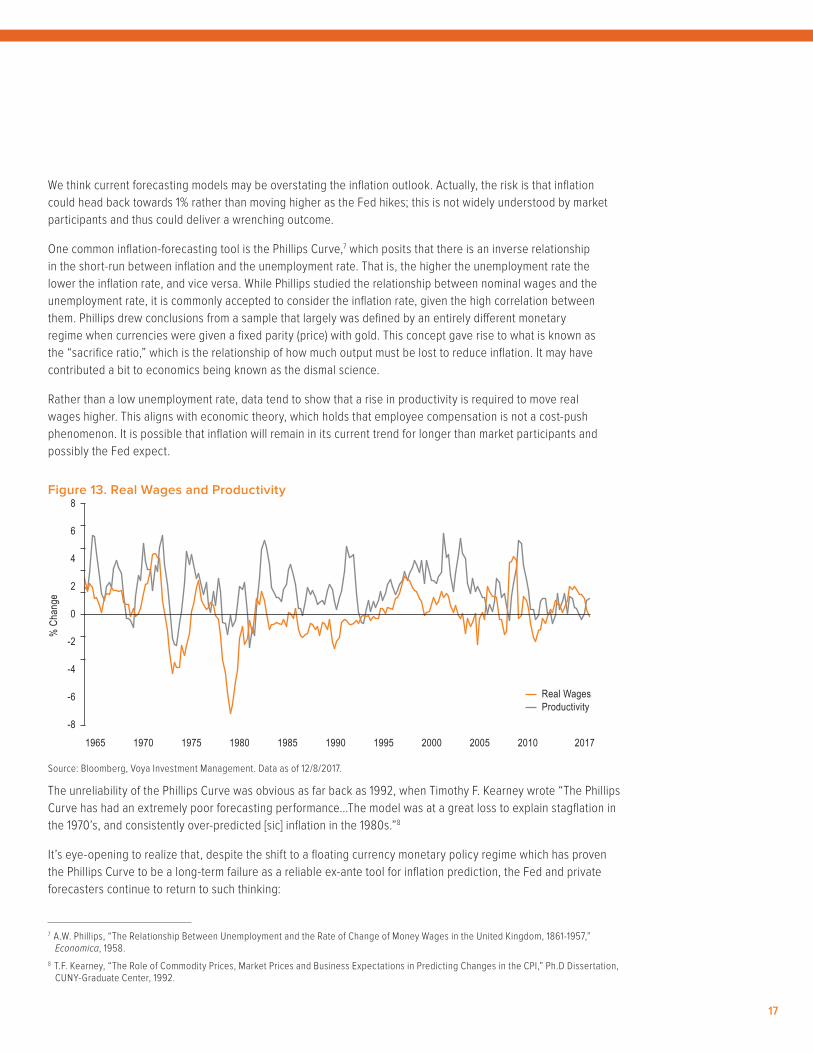
Rather than a low unemployment rate, data tend to show that a rise in productivity is required to move real wages higher. This aligns with economic theory, which holds that employee compensation is not a cost-push phenomenon. It is possible that inflation will remain in its current trend for longer than market participants and possibly the Fed expect.

Figure 13. Real Wages and Productivity

Source: Bloomberg, Voya Investment Management. Data as of 12/8/2017.

The unreliability of the Phillips Curve was obvious as far back as 1992, when Timothy F. Kearney wrote “The Phillips Curve has had an extremely poor forecasting performance…The model was at a great loss to explain stagflation in the 1970’s, and consistently over-predicted [sic] inflation in the 1980s.”8

It’s eye-opening to realize that, despite the shift to a floating currency monetary policy regime which has proven the Phillips Curve to be a long-term failure as a reliable ex-ante tool for inflation prediction, the Fed and private forecasters continue to return to such thinking:

7 A.W. Phillips, “The Relationship Between Unemployment and the Rate of Change of Money Wages in the United Kingdom, 1861-1957,” Economica, 1958.

8 T.F. Kearney, “The Role of Commodity Prices, Market Prices and Business Expectations in Predicting Changes in the CPI,” Ph.D Dissertation, CUNY-Graduate Center, 1992.

1965 19751970 1980 1990 20001985 1995 2005 2010 2017

Real WagesProductivity

-6

-4

-2

-8

0

2

4

6

8

% C

hang

e

18

■ In an important review of inflation, Steven Ceccehti et. al.9 “We then ask if the deviation of inflation from the recursive estimate of the local mean is related to either the deviation of inflation expectations from that same mean, or to the unemployment gap (once we control for the lagged deviation of inflation from the local mean that our model tells us is present). …we find neither inflation expectations nor labor market slack help us to explain quarter-to-quarter deviations of inflation from its local mean.”

■ Robert Gordon10: “Has the slope of the American Phillips Curve flattened in the past two decades? Research at the Federal Reserve believes so.”

■ Janet Yellen11: “A more important issue from a policy standpoint is that some key assumptions underlying the baseline outlook could be wrong in ways that imply that inflation will remain low for longer than currently projected. For example, labor market conditions may not be as tight as they appear to be, and thus they may exert less upward pressure on inflation than anticipated.”

Dr. Yellen’s 2017 speech gives rise to an intriguing idea: the model she puts forward is self-fulfilling.

Her model is based on a) expected long-run inflation, b) slack and c) import prices. She defines “slack” as the level of resource utilization, i.e., “…(for) estimation purposes, slack is approximated using the unemployment rate less the Congressional Budget Office’s (CBO) historical series for the long-run natural rate.”

In a sense the Fed perceives the amount of slack it sets. She offered that “On balance, the unemployment rate probably is correct in signaling that overall labor market conditions have returned to pre-crisis levels. But that return does not necessarily demonstrate that the economy is now at maximum employment because, due to demographic and other structural changes, the unemployment rate that is sustainable today may be lower than the rate that was sustainable in the past.”

What the Data SaySince 1945, a case can be made that inflation occurs only when major disequilibria persist. That is, the “natural state” for inflation is a flat, average inflation rate tied to expectations. Using the CPI (data which begin in the 1930s), we look at four periods: The immediate post-war eras covering the end of both World War II and of the Korean conflict, the Bretton Woods system working, post Bretton Woods adjustment and the current credible Fed period. The data show that as long as expectations are grounded and the Fed is credible, the inflation rate will not exceed the target, absent a major disruption. Let’s take a look at each in turn.

9 S. Cecchetti, M. Feroli, P. Hooper, A. Kashyap and K. Schoenholtz, “Deflating Inflation Expectations: The Implications of Inflation’s Simple Dynamics,” at the U.S. Monetary Forum, 2017.

10 R. Gordon, “The Phillips Curve Is Alive and Well: Inflation and the NAIRU During the Slow Recovery,” NBER Working Paper # 19390, 2013.11 J. Yellen, “Inflation, Uncertainty and Monetary Policy,” Annual Meeting of NABE, Cleveland, OH, 2017.

19

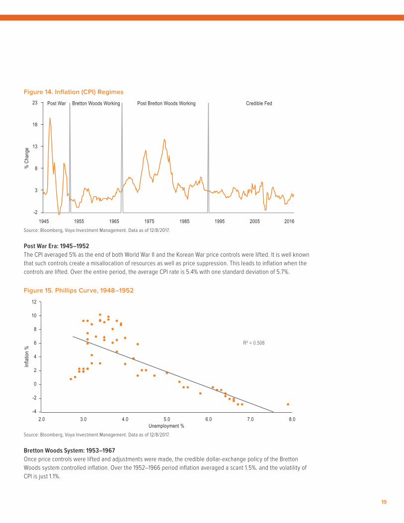
Figure 14. Inflation (CPI) Regimes


Post War Era: 1945–1952The CPI averaged 5% as the end of both World War II and the Korean War price controls were lifted. It is well known that such controls create a misallocation of resources as well as price suppression. This leads to inflation when the controls are lifted. Over the entire period, the average CPI rate is 5.4% with one standard deviation of 5.7%.

Figure 15. Phillips Curve, 1948–1952


Bretton Woods System: 1953–1967Once price controls were lifted and adjustments were made, the credible dollar-exchange policy of the Bretton Woods system controlled inflation. Over the 1952–1966 period inflation averaged a scant 1.5%. and the volatility of CPI is just 1.1%.

% C

hang

e

Post War Bretton Woods Working Post Bretton Woods Working Credible Fed

-2

3

8

13

18

23

1945 1955 1975 19951965 1985 2005 2016

Infla

tion

%

Unemployment %

R² = 0.508

-4

-2

0

2

4

6

8

10

12

2.0 3.0 4.0 5.0 6.0 7.0 8.0

20

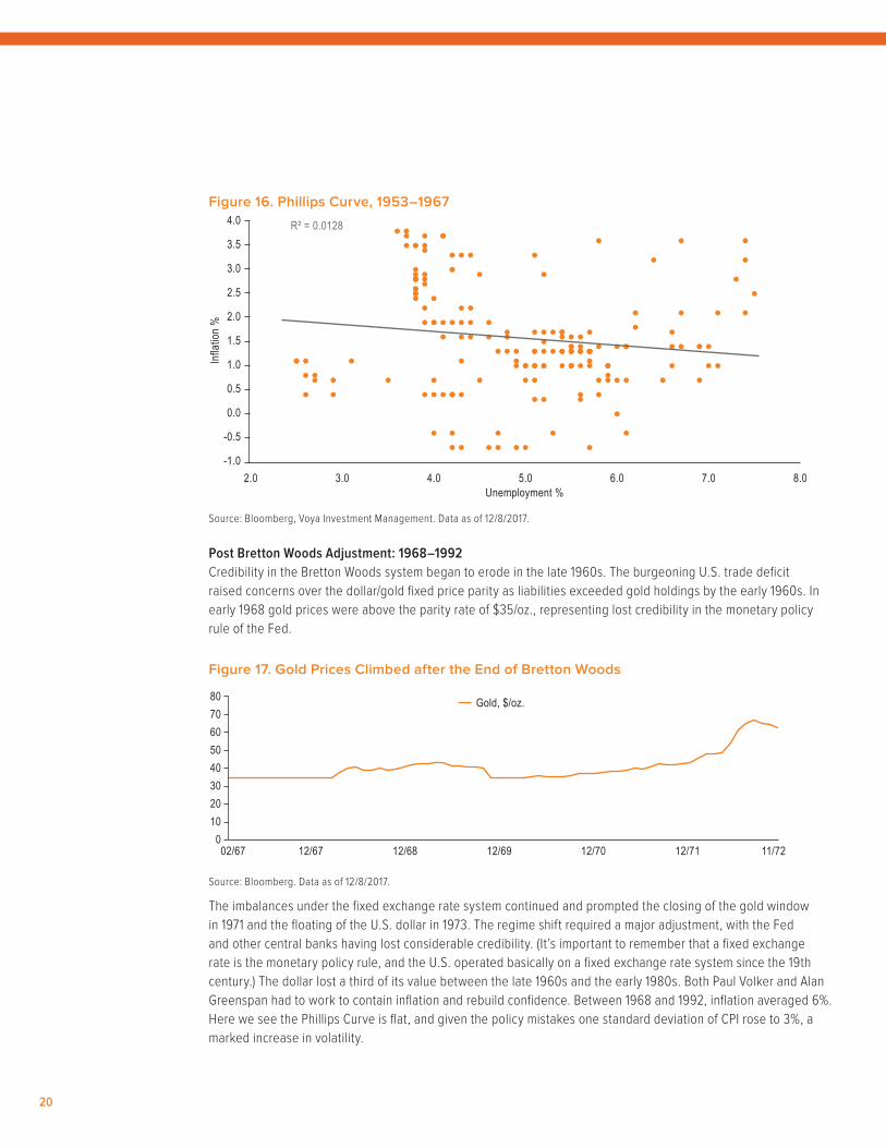
Figure 16. Phillips Curve, 1953–1967


Post Bretton Woods Adjustment: 1968–1992Credibility in the Bretton Woods system began to erode in the late 1960s. The burgeoning U.S. trade deficit raised concerns over the dollar/gold fixed price parity as liabilities exceeded gold holdings by the early 1960s. In early 1968 gold prices were above the parity rate of $35/oz., representing lost credibility in the monetary policy rule of the Fed.

Figure 17. Gold Prices Climbed after the End of Bretton Woods

Source: Bloomberg. Data as of 12/8/2017.

The imbalances under the fixed exchange rate system continued and prompted the closing of the gold window in 1971 and the floating of the U.S. dollar in 1973. The regime shift required a major adjustment, with the Fed and other central banks having lost considerable credibility. (It’s important to remember that a fixed exchange rate is the monetary policy rule, and the U.S. operated basically on a fixed exchange rate system since the 19th century.) The dollar lost a third of its value between the late 1960s and the early 1980s. Both Paul Volker and Alan Greenspan had to work to contain inflation and rebuild confidence. Between 1968 and 1992, inflation averaged 6%. Here we see the Phillips Curve is flat, and given the policy mistakes one standard deviation of CPI rose to 3%, a marked increase in volatility.

Infla

tion

%

Unemployment %

R² = 0.0128

2.0 3.0 4.0 5.0 6.0 7.0 8.0-1.0

-0.5

0.0

0.5

1.0

1.5

2.0

2.5

3.0

3.5

4.0

02/67 12/67 12/68 12/69 12/70 12/71 11/720

2030

10

4050607080 Gold, $/oz.

21

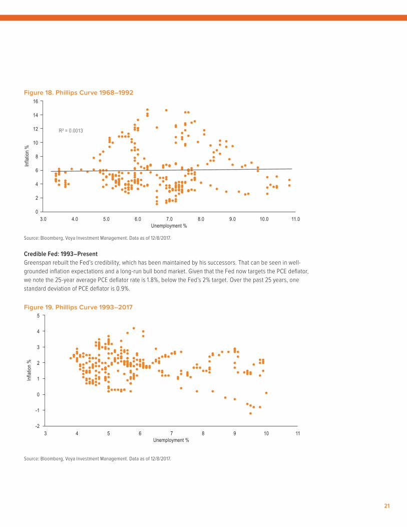
Figure 18. Phillips Curve 1968–1992


Credible Fed: 1993–PresentGreenspan rebuilt the Fed’s credibility, which has been maintained by his successors. That can be seen in well-grounded inflation expectations and a long-run bull bond market. Given that the Fed now targets the PCE deflator, we note the 25-year average PCE deflator rate is 1.8%, below the Fed’s 2% target. Over the past 25 years, one standard deviation of PCE deflator is 0.9%.

Figure 19. Phillips Curve 1993–2017


Infla

tion

%

Unemployment %

R² = 0.0013

3.0 4.0 5.0 6.0 7.0 8.0 9.0 10.0 11.00

2

4

6

8

10

12

14

16

Infla

tion

%

Unemployment %3 4 5 6 7 8 9 10 11

-2

-1

0

1

2

3

4

5

22

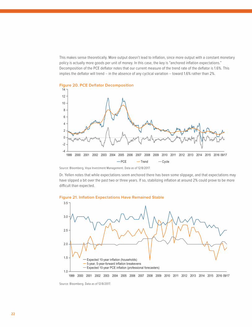
This makes sense theoretically. More output doesn’t lead to inflation, since more output with a constant monetary policy is actually more goods per unit of money. In this case, the key is “anchored inflation expectations.” Decomposition of the PCE deflator notes that our current measure of the trend rate of the deflator is 1.6%. This implies the deflator will trend – in the absence of any cyclical variation – toward 1.6% rather than 2%.

Figure 20. PCE Deflator Decomposition


Dr. Yellen notes that while expectations seem anchored there has been some slippage, and that expectations may have slipped a bit over the past two or three years. If so, stabilizing inflation at around 2% could prove to be more difficult than expected.

Figure 21. Inflation Expectations Have Remained Stable

Source: Bloomberg. Data as of 12/8/2017.

1999 2016 09/17

PCE Cycle

-4

0

-2

4

2

8

6

12

10

14

2015201420132012201120102009200820072006200520042003200220012000

Trend

1999 2016 09/17

Expected 10-year inflation (households)5-year, 5-year-forward inflation breakevensExpected 10-year PCE inflation (professional forecasters)

1.0

1.5

2.0

2.5

3.0

3.5

2015201420132012201120102009200820072006200520042003200220012000

23

In short, our analysis points away from labor market/Phillips Curve types of relationships as the driver of inflation. Economists may be able to tease a Phillips Curve ex-post; however, that doesn’t mean that the Phillips Curve is an exploitable, ex-ante forecasting tool. Gregory Mankiw12 notes that, with the imposing credible policies some research points to rational actors lowering “…their expectations of inflation immediately. The short-run Phillips curve would shift downward, and the economy would reach low inflation quickly without the cost of temporarily high unemployment and low output.” Likely to prove more important to the inflation outlook is the shift to a new Fed chair and new members on the FOMC. Clearly, Dr. Yellen’s policies have proven to be credible and contained inflation. It will be up to the new chair, Jerome Powell, and his new team, including his as-yet unnamed vice chair, to deliver a credible message to economic actors and nudge inflation towards the target 2% PCE deflator inflation rate.

12 G. Mankiw, Principles of Economics, 7th edition, 2015.

24

Methodological Considerations

Covariance and Correlation Matrices MethodologyEstimating asset-class covariance and correlation matrices are the underlying pillars of our asset-class standard deviation forecasts. This is a different process than forecasting returns, as evidence tells us that correlations wander through time. If we were to use a historical average or exponentially weighted methodology, which takes a long-run history and puts a heavier weight on recent observations, it could lead to risk forecasts that may be representative of the past but bear little resemblance to the future. Therefore, the forecast multiple asset-class risk summarized by the return covariance matrix is crucial to the capital market assumptions process.

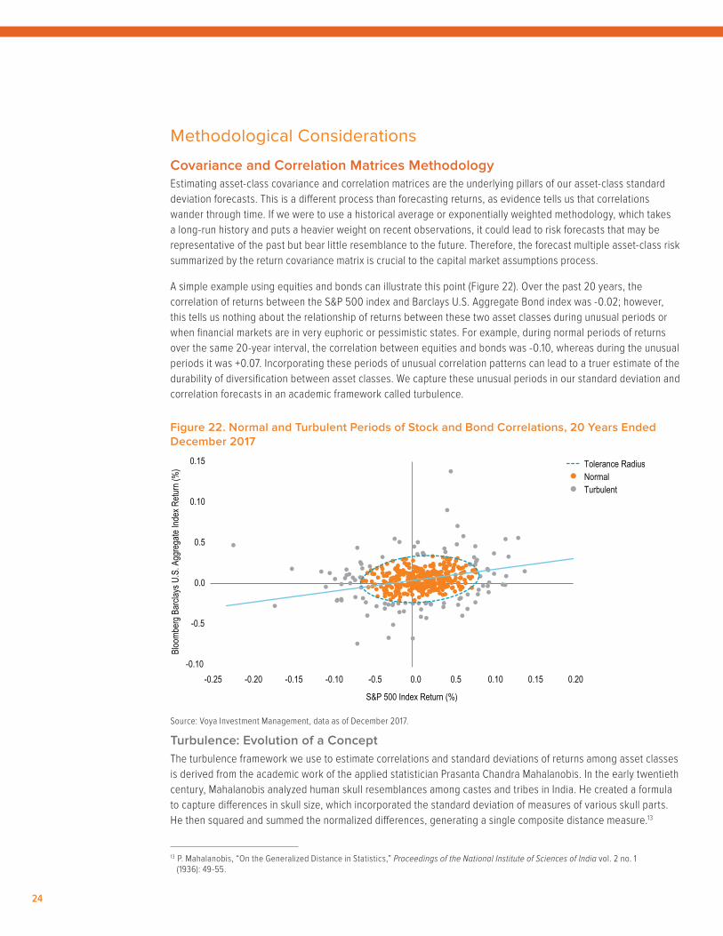
A simple example using equities and bonds can illustrate this point (Figure 22). Over the past 20 years, the correlation of returns between the S&P 500 index and Barclays U.S. Aggregate Bond index was -0.02; however, this tells us nothing about the relationship of returns between these two asset classes during unusual periods or when financial markets are in very euphoric or pessimistic states. For example, during normal periods of returns over the same 20-year interval, the correlation between equities and bonds was -0.10, whereas during the unusual periods it was +0.07. Incorporating these periods of unusual correlation patterns can lead to a truer estimate of the durability of diversification between asset classes. We capture these unusual periods in our standard deviation and correlation forecasts in an academic framework called turbulence.

Figure 22. Normal and Turbulent Periods of Stock and Bond Correlations, 20 Years Ended December 2017

Source: Voya Investment Management, data as of December 2017.

Turbulence: Evolution of a ConceptThe turbulence framework we use to estimate correlations and standard deviations of returns among asset classes is derived from the academic work of the applied statistician Prasanta Chandra Mahalanobis. In the early twentieth century, Mahalanobis analyzed human skull resemblances among castes and tribes in India. He created a formula to capture differences in skull size, which incorporated the standard deviation of measures of various skull parts. He then squared and summed the normalized differences, generating a single composite distance measure.13

13 P. Mahalanobis, “On the Generalized Distance in Statistics,” Proceedings of the National Institute of Sciences of India vol. 2 no. 1 (1936): 49-55.

-0.10

-0.5

0.0

0.5

0.10

0.15

-0.25 -0.20 -0.15 -0.10 -0.5 0.0 0.5 0.10 0.15 0.20

Bloo

mber

g Bar

clays

U.S

. Agg

rega

te Ind

ex R

eturn

(%)

S&P 500 Index Return (%)

Tolerance RadiusNormalTurbulent

25

This formula evolved into a statistical measure called the “Mahalanobis distance.” The measure was ground-breaking in that it helped analyze data across standard deviations but also incorporated the correlations among data sets. More than 60 years later, the Mahalanobis distance was used by Kritzman and Li to formulate a concept called financial turbulence.14 They postulated financial turbulence as a condition in which asset prices, given their historical patterns of returns, behave in an uncharacteristic way including extreme price moves. They further noted that financial turbulence often coincides with excessive risk aversion, illiquidity and price declines for risky assets. It is this turbulence framework (or unusualness of returns and correlations of returns) that we have used to forecast risk measures in our capital market assumptions.

Observing TurbulenceTurbulence can be calculated for any given set of asset classes. Back to our example of U.S. equities and bonds, the two dimensions can be visualized as the equation of an ellipse using the returns of the S&P 500 index and the U.S. Barclays Aggregate index (Figure 22). The center of the ellipse represents the average of the joint returns of the two assets. The boundary is a level of tolerance that separates normal from turbulent observations. The boundary takes the form of an ellipse rather than a circle because it takes into account the covariance of the asset classes. The idea captured by this measure is that certain periods are considered turbulent not only because returns are unusually high or low but also because they moved in the opposite direction of what would have been expected given average correlations.

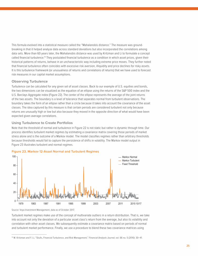
Using Turbulence to Create Portfolios Note that the threshold of normal and turbulence in Figure 22 is not static but rather is dynamic through time. Our process identifies turbulent market regimes by estimating a covariance matrix covering those periods of market stress alone and is the outcome of a Markov model. The model classifies regimes rather than arbitrary thresholds because thresholds would fail to capture the persistence of shifts in volatility. The Markov model output in Figure 23 illustrates turbulent and normal regimes.

Figure 23. Markov 12-Asset Normal and Turbulent Regimes

Source: Voya Investment Management, data as of October 2017.

Turbulent market regimes make use of the concept of multivariate outliers in a return distribution. That is, we take into account not only the deviation of a particular asset class’s return from the average, but also its volatility and correlation with other asset classes. We subsequently estimate a covariance matrix based on periods of normal and turbulent market performance. Finally, we use a procedure to blend these two covariance matrices using

14 M. Kritzman and Y. Li, “Skulls, Financial Turbulence, and Risk Management,” Financial Analysts Journal, vol. 66 no. 5 (2010): 30–41.

01979 1983 1987 1991 1995 1999 2003 2007 2011 10/172015

20

60

Markov NormalMarkov TurbulentFixed Threshold

40

80

100

26

weights that allow us to express both views about the likelihood of each normal or turbulent regime and to capture the differential risk attitudes toward each. The weights we use are 60% normal and 40% turbulent to create our strategic asset allocation portfolios.

We overweight the turbulent regime at 40% — higher than its observed frequency of 30% — to account for structural issues such as globalization, demographics and worldwide central bank intervention, which are prevalent today. From this blended covariance matrix, we then extract the implied correlation matrix and standard deviations for each asset class. In our view, this process helps create a strategic asset allocation portfolio that can account for the empirical evidence that correlations will deviate through time.

Time Dependency of Asset Returns and Its Impact on Risk Estimation Recent research suggests that expected asset returns change over time in somewhat predictable ways and that these changes tend to persist over long periods. Thus, changes among investment opportunities — all possible combinations of risk and return — are found to be persistent. This Appendix will set out the economic reasons for return predictability, its consequences for strategic asset allocation and the adjustments we have made to control for it in our estimation process.

In our view, the common source of predictability in financial asset returns is the business cycle. The business cycle itself is persistent, and this makes real economic growth to some extent predictable. The fundamental reason for the business cycle’s persistence is that its components share the same quality. Consumers, for example, have a tendency to smooth consumption since they dislike abrupt changes in their lifestyles. Research on permanent income and lifecycle consumption provides the theoretical basis for consumers’ desire for a stable consumption path. When income is affected by transitory shocks, consumption should not change since consumers can use savings or borrowing to adjust consumption in well-functioning capital markets.

Robert Hall has formalized these ideas by showing that consumers will optimally choose to keep a stable path of consumption equal to a fraction of their present discounted value of human and financial wealth.15 Investment, the second component of GDP, is sticky, as corporate investment in projects is usually long-term in nature. Finally, government expenditures also have a low level of variability. Over a medium-term horizon, negative serial correlation sets in as the growth phase of the cycle is followed by a contraction and then that contraction is followed by renewed growth.16

How does this predictability of economic variables affect the predictability of asset returns? Consider equities as an example. The value of equities is determined as the present discounted value of future cash flows and depends on four factors: expected cash flows, expected market risk premium, expected market risk exposure and the term structure of interest rates. Cash flows and corporate earnings tend to move with the business cycle. The market risk premium is high at business cycle troughs, when consumers are trying to smooth consumption and are less willing to take risks with their income; and low at business cycle peaks, when people are more willing to take risks. The market risk premium is a component of the discount rate in the present value calculation of the dividend discount model. A firm’s risk exposure (beta), another component of the discount rate, changes through time and is a function of its capital structure. Thus, a firm’s risk increases with leverage, which is related to the business cycle. The last component of the discount rate is the risk-free rate, which is determined by the term structure of interest rates. The term structure reflects expectations of real interest rates, real economic activity and inflation, which are connected to the business cycle. Thus, equity returns, and financial asset returns in general, are to a certain extent

15 R. Hall, “Stochastic Implications of the Life-Cycle-Permanent Income Hypothesis: Theory and Evidence,” Journal of Political Economy 86 (1978): 971–988.

16 J. Poterba and L. Summers, “Mean Reversion in Stock Prices: Evidence and Implications,” Journal of Financial Economics 22 (1988): 27–60.

27

predictable. Expected returns of many assets tend to be high in bad macroeconomic times and low in good times.

This predictability of returns manifests itself statistically through autocorrelation. Autocorrelation in time series of returns describes the correlation between values of a return process at different points in time. Autocorrelation can be positive when high returns tend to be followed by high returns, implying momentum in the market. Conversely, negative autocorrelation occurs when high returns tend to be followed by low returns, implying mean reversion. In either case autocorrelation induces dependence in returns over time.

Traditional mean-variance analysis focused on short-term expected return and risk assumes returns do not exhibit time dependence and prices follow a random walk. Expected returns in a random walk are constant, exhibiting zero autocorrelation; realized short-term returns are not predictable. Volatilities and cross-correlations among assets are independent of the investment horizon. Thus, the annualized volatility estimated from monthly return data scaled by the square root of 12 should be equal to the volatility estimated from quarterly return data scaled by the square root of four. In the presence of autocorrelation, the square root of time scaling rule described above is not valid, since the sample standard deviation estimator is biased and the sign of autocorrelation matters for its impact on volatility and correlations. Positive autocorrelation leads to an underestimation of true volatility.

A similar result holds for the cross-correlation matrix bias when returns exhibit autocorrelation. So for long investment horizons, the risk/return tradeoff can be very different than that for short investment horizons.

In a multi-asset portfolio, in which different asset classes display varying degrees of autocorrelation, failure to correct for the bias of volatilities and correlations will lead to suboptimal mean variance optimized portfolios in which asset classes that appear to have low volatilities receive excessive allocations. Such asset classes include hedge funds, emerging market equities and non-public market assets such as private equity or private real estate, among others.

There are at least two ways to correct for autocorrelation: ■ A direct method that adjusts the sample estimators of volatility, correlation and all higher moments

■ An indirect method that cleans the data first, allowing us to subsequently estimate the moments of the distribution using standard estimators

Given that the direct methods become quite complex beyond the first two moments, our choice is to follow the second method and clean the return data of autocorrelation. Before we do that we estimate and test the statistical significance of autocorrelation in our data series.

We estimate first-order autocorrelation correlation as the regression slope of a first-order autoregressive process. We use monthly return data for the period 1979–2014. We subsequently test the statistical significance of the estimated parameter using the Ljung-Box Q-statistic.17 The Q-statistic is a statistical test for serial correlation at any number of lags. It is distributed as a chi-square with k degrees of freedom, where k is the number of lags. Here we test for first-order serial correlation, thus k = 1. About 80% of our return series exhibit positive and statistically significant first-order serial correlation based on associated p-values at the 10% level of significance.18 Khandani and Lo provide empirical evidence that positive return autocorrelation is a measure of illiquidity exhibited among a broad set of financial assets including small-cap stocks, corporate bonds, mortgage-backed securities and

17 G.M. Ljung and G.E.P. Box, “On a Measure of Lack of Fit in Time Series Models,” Biometrika, 65, (1978): 297–303.18 The p-value is the probability of rejecting the null hypothesis of no serial correlation when it is true (i.e., concluding that there is serial

correlation in the data when in fact serial correlation does not exist). We set critical values at 10% and thus reject the null hypothesis of no serial correlation for p-values <10%.

©2018 Voya Investments Distributor, LLC • 230 Park Ave, New York, NY 10169 • All rights reserved.

BSWP-CMA 021218 • IM1215-39095-1218 • 167284

Past performance does not guarantee future results.

This commentary has been prepared by Voya Investment Management for informational purposes. Nothing contained herein should be construed as (i) an offer to sell or solicitation of an offer to buy any security or (ii) a recommendation as to the advisability of investing in, purchasing or selling any security. Any opinions expressed herein reflect our judgment and are subject to change. Certain of the statements contained herein are statements of future expectations and other forward-looking statements that are based on management’s current views and assumptions and involve known and unknown risks and uncertainties that could cause actual results, performance or events to differ materially from those expressed or implied in such statements. Actual results, performance or events may differ materially from those in such statements due to, without limitation, (1) general economic conditions, (2) performance of financial markets, (3) interest rate levels, (4) increasing levels of loan defaults, (5) changes in laws and regulations, and (6) changes in the policies of governments and/or regulatory authorities.

The opinions, views and information expressed in this commentary regarding holdings are subject to change without notice. The information provided regarding holdings is not a recommendation to buy or sell any security. Fund holdings are fluid and are subject to daily change based on market conditions and other factors.

For Australian Investors

Voya Investment Management Co. LLC (“Voya”) is exempt from the requirement to hold an Australian financial services license under the Corporations Act 2001 (Cth) (“Act”) in respect of the financial services it provides in Australia. Voya is regulated by the SEC under U.S. laws, which differ from Australian laws.

This document or communication is being provided to you on the basis of your representation that you are a wholesale client (within the meaning of section 761G of the Act), and must not be provided to any other person without the written consent of Voya, which may be withheld in its absolute discretion.

emerging market investments.19 The theoretical basis is that in a frictionless market, any predictability in asset returns can be immediately exploited, thus eliminating such predictability. While other measures of illiquidity exist, autocorrelation is the only measure that applies to both publicly and privately traded securities and requires only returns to compute.

Since the vast majority of the return series we estimate exhibit autocorrelation, we apply the Geltner unsmoothing process to all series. This process corrects the return series for first-order serial correlation by subtracting the product of the autocorrelation coefficient ρ and the previous period’s return from the current period’s return and dividing by 1-ρ. This transformation has no impact on the arithmetic return, but the geometric mean is impacted since it depends on volatility. This correction is thus important to make for long-horizon asset allocation portfolios.

New York City December 2017

Multi-Asset Strategies and Solutions TeamVoya Investment Management’s Multi-Asset Strategies and Solutions (MASS) team, led by Chief Investment Officer Paul Zemsky, manages the firm’s suite of multi-asset solutions designed to help investors achieve their long-term objectives. The team consists of 25 investment professionals that have deep expertise in asset allocation, manager selection and research, quantitative research, portfolio implementation and actuarial sciences. Within MASS, the asset allocation team, led by Barbara Reinhard, is responsible for constructing strategic asset allocations based on their long-term views. The team also employs a tactical asset allocation approach, driven by market fundamentals, valuation and sentiment, which is designed to capture market anomalies and/or reduce portfolio risk.

19 A.E. Khandani and A. Lo, “Illiquidity Premia in Asset Returns: An Empirical Analysis of Hedge Funds, Mutual Funds, and U.S. Equity Portfolios,” Quarterly Journal of Finance 1 (2011): 205–264.

Documents

2018 Capital Market Assumptions - institutional.voya.com 3 Executive Summary Our 2018 Long Term Capital Market Assumptions details our Voya capital markets forecasts of asset class