3. Stochastic Processes

We learn in kindergarten about the phenomenon of Brownian motion, the random

jittery movement that a particle suffers when it is placed in a liquid. Famously, it is

caused by the constant bombardment due to molecules in the surrounding the liquid.

Our goal in this section is to introduce the mathematical formalism that allows us to

model such random behaviour.

3.1 The Langevin Equation

In contrast to the previous section, we will here focus on just a single particle. However,

this particle will be sitting in a background medium. If we know the force F acting on

the particle, its motion is entirely deterministic, governed by

m~x = −γ~x+ ~F (3.1)

In contrast to the previous section, this is not a Hamiltonian system. This is because

we have included a friction term with a coefficient γ. This arises due to the viscosity, η,

of the surrounding liquid that we met in the previous section. If we model the particle

as a sphere of radius a then there is a formula due to Stokes which says γ = 6πηa.

However, in what follows we shall simply treat γ as a fixed parameter. In the presence

of a time independent force, the steady-state solution with ~x = 0 is

~x =1

γ~F

For this reason, the quantity 1/γ is sometimes referred to as the mobility.

Returning to (3.1), for any specified force ~F , the path of the particle is fully deter-

mined. This is seemingly at odds with the random behaviour observed in Brownian

motion. The way in which we reconcile these two points is, hopefully, obvious: in

Brownian motion the force ~F that the particle feels is itself random. In fact, we will

split the force into two pieces,

~F = −∇V + ~f(t)

Here V is a fixed background potential in which the particle is moving. Perhaps V

arises because the particle is moving in gravity; perhaps because it is attached to a

spring. But, either way, there is nothing random about V . In contrast, ~f(t) is the

random force that the particle experiences due to all the other atoms in the liquid. It is

sometimes referred to as noise. The resulting equation is called the Langevin equation

m~x = −γ~x−∇V + ~f(t) (3.2)

– 52 –

Although it looks just like an ordinary differential equation, it is, in fact, a different

beast known as a stochastic differential equation. The reason that it’s different is that

we don’t actually know what ~f(t) is. Yet, somehow, we must solve this equation

anyway!

Let’s clarify what is meant by this. Suppose that you did know the microscopic

force ~f(t) that is experienced by a given particle. Then you could, in principle, go

ahead and solve the Langevin equation (3.2). But the next particle that you look at

will experience a different force ~f(t) so you’ll have to solve (3.2) again. And for the

third particle, you’ll have to solve it yet again. Clearly, this is going to become tedious.

What’s more, it’s unrealistic to think that we will actually know ~f(t) in any specific

case. Instead, we admit that we only know certain crude features of the force ~f(t)

such as, for example, its average value. Then we might hope that this is sufficient

information to figure out, say, the average value of ~x(t). That is the goal when solving

the Langevin equation.

3.1.1 Diffusion in a Very Viscous Fluid

We start by solving the Langevin equation in the case of vanishing potential, V =

0. (For an arbitrary potential, the Langevin equation is an unpleasant non-linear

stochastic differential equation and is beyond our ambition in this course. However, we

will discuss some properties of the case with potential is the following section when we

introduce the Fokker-Planck equation). We can simplify the problem even further by

considering Brownian motion in a very viscous liquid. In this case, motion is entirely

dominated by the friction term in the Langevin equation and we ignore the inertial

term, which is tantamount to setting m = 0.

When m = 0, we’re left with a first order equation,

~x(t) =1

γ~f(t)

For any ~f(t), this can be trivially integrated to give

~x(t) = ~x(0) +1

γ

∫ t

0

dt′ ~f(t′) (3.3)

At this point, we can’t go any further until we specify some of the properties of the

noise ~f(t). Our first assumption is that, on average, the noise vanishes at any given

time. We will denote averages by 〈 · 〉, so this assumption reads

〈~f(t)〉 = 0 (3.4)

– 53 –

Taking the average of (3.3) then gives us the result:

〈~x(t)〉 = ~x(0)

The is deeply unsurprising: if the average noise vanishes, the average position of the

particle is simply where we left it to begin with. Nonetheless, it’s worth stressing that

this doesn’t mean that all particles sit where you leave them. It means that, if you drop

many identical particles at the origin, ~x(0) = ~0, they will all move but their average

position — or their centre of mass — will remain at the origin.

We can get more information by looking at the variance of the position,

〈 (~x(t) − ~x(0))2 〉

This will tell us the average spread of the particles. We can derive an expression for

the variance by first squaring (3.3) and then taking the average,

〈 (~x(t) − ~x(0))2 〉 =1

γ2

∫ t

0

dt′1

∫ t

0

dt′2 〈 ~f(t′1) · ~f(t′2) 〉 (3.5)

In order to compute this, we need to specify more information about the noise, namely

its correlation function 〈 fi(t1)fj(t2) 〉 where we have resorted to index notation, i, j =

1, 2, 3 to denote the direction of the force. This is specifying how likely it is that the

particle will receive a given kick fj at time t2 given that it received a kick fi at time t1.

In many cases of interest, including that of Brownian motion, the kicks imparted by

the noise are both fast and uncorrelated. Let me explain what this means. Suppose

that a given collision between our particle and an atom takes time τcoll. Then if we

focus on time scales less than τcoll then there will clearly be a correlation between the

forces imparted on our particle because these forces are due to the same process that’s

already taking place. (If an atom is coming in from the left, then it’s still coming in

from the left at a time t≪ τcoll later). However if we look on time scales t≫ τcoll, the

force will be due to a different collision with a different atom. The statement that the

noise is uncorrelated means that the force imparted by later collisions knows nothing

about earlier collisions. Mathematically, this means

〈 fi(t1)fj(t2) 〉 = 0 when t2 − t1 ≫ τcoll

The statement that the collisions are fast means that we only care about time scales

t2 − t1 ≫ τcoll and so can effectively take the limit τcoll → 0. However, that doesn’t

– 54 –

quite mean that we can just ignore this correlation function. Instead, when we take

the limit τcoll → 0, we’re left with a delta-function contribution,

〈 fi(t1)fj(t2) 〉 = 2Dγ2 δij δ(t2 − t1) (3.6)

Here the factor of γ2 has been put in for convenience. We will shortly see the inter-

pretation of the coefficient D, which governs the strength of the correlations. Noise

which obeys (3.4) and (3.6) is often referred to as white noise. It is valid whenever the

environment relaxes back down to equilibrium much faster than the system of interest.

This guarantees that, although the system is still reeling from the previous kick, the

environment remembers nothing of what went before and kicks again, as fresh and

random as the first time.

Using this expression for white noise, the variance (3.5) in the position of the particles

is

〈 (~x(t) − ~x(0))2 〉 = 6D t (3.7)

This is an important result: the root-mean square of the distance increases as√t with

time. This is characteristic behaviour of diffusion. The coefficient D is called the

diffusion constant. (We put the factor of γ2 in the correlation function (3.6) so that

this equation would come out nicely).

3.1.2 Diffusion in a Less Viscous Liquid

Let’s now return to the Langevin equation (3.2) and repeat our analysis, this time

retaining the inertia term, so m 6= 0. We will still set V = 0.

As before, computing average quantities — this time both velocity 〈 ~x(t) 〉 and posi-

tion 〈 ~x(t) 〉 is straightforward and relatively uninteresting. For a given ~f(t), it is not

difficult to solve (3.2). After multiplying by an integrating factor eγt/m, the equation

becomes

d

dt

(

~xeγt/m)

=1

m~f(t)eγt/m

which can be happily integrated to give

~x(t) = ~x(0)e−γt/m +1

m

∫ t

0

dt′ ~f(t′) eγ(t′−t)/m (3.8)

We now use the fact that the average of noise vanishes (3.4) to find that the average

velocity is simply that of a damped particle in the absence of any noise,

〈~x(t)〉 = ~x(0)e−γt/m

– 55 –

Similarly, to determine the average position we have

~x(t) = ~x(0) +

∫ t

0

dt′ ~x(t′) (3.9)

From which we get

〈~x(t)〉 = ~x(0) +

∫ t

0

dt′ 〈~x(t′)〉

= ~x(0) +m

γ~x(0)

(

1 − e−γt/m)

Again, this is unsurprising: when the average noise vanishes, the average position of

the particle coincides with that of a particle that didn’t experience any noise.

Things get more interesting when we look at the expectation values of quadratic

quantities. This includes the variance in position 〈 ~x(t) ·~x(t) 〉 and velocity 〈 ~x(t) · ~x(t) 〉,but also more general correlation functions in which the two quantities are evaluated at

different times. For example, the correlation function 〈 xi(t1)xj(t2) 〉 tells us information

about the velocity of the particle at time t2 given that we know where its velocity at

time t1. From (3.8), we have the expression,

〈xi(t1)xj(t2)〉 = 〈 xi(t1) 〉〈 xj(t2) 〉 +1

m2

∫ t1

0

dt′1

∫ t2

0

dt′2 〈fi(t′

1)fj(t′

2)〉 eγ(t′1+t′

2−t1−t2)/m

where we made use of the fact that 〈~f(t)〉 = 0 to drop the terms linear in the noise~f . If we use the white noise correlation function (3.6), and assume t2 ≥ t1 > 0, the

integral in the second term becomes,

〈xi(t1)xj(t2)〉 = 〈 xi(t1) 〉〈 xj(t2) 〉 +2Dγ2

m2δij e

−γ(t1+t2)/m

∫ t1

0

dt′ e2γt′/m

= 〈 xi(t1) 〉〈 xj(t2) 〉 +Dγ

mδij(

e−γ(t2−t1)/m − e−γ(t1+t2)/m)

For very large times, t1, t2 → ∞, we can drop the last term as well as the average

velocities since 〈 ~x(t) 〉 → 0. We learn that the correlation between velocities decays

exponentially as

〈xi(t1)xj(t2)〉 →Dγ

mδij e

−γ(t2−t1)/m

This means that if you know the velocity of the particle at some time t1, then you can

be fairly confident that it will have a similar velocity at a time t2 < t1 + m/γ later.

But if you wait longer than time m/γ then you would be a fool to make any bets on

the velocity based only on your knowledge at time t1.

– 56 –

Finally, we can also use this result to compute the average velocity-squared (which,

of course, is the kinetic energy of the system). At late times, the any initial velocity

has died away and the resulting kinetic energy is due entirely to the bombardment by

the environment. It is independent of time and given by

〈~x(t) · ~x(t) 〉 =3Dγ

m(3.10)

One can compute similar correlation functions for position 〈 xi(t1)xj(t2) 〉. The ex-

pressions are a little more tricky but still quite manageable. (Combining equations

(3.9) and (3.8), you can see that you will a quadruple integral to perform and figuring

out the limits is a little fiddly). At late times, it turns out that the variance of the

position is given by the same expression that we saw for the viscous liquid (3.7),

〈 (~x(t) − ~x(0))2 〉 = 6D t (3.11)

again exhibiting the now-familiar√t behaviour for the root-mean-square distance.

3.1.3 The Einstein Relation

We brushed over something important and lovely in the previous discussion. We com-

puted the average kinetic energy of a particle in (3.10). It is

E =1

2m〈~x · ~x 〉 =

3

2Dγ

But we already know what the average energy of a particle is when it’s bombarded by

its environment: it is given by the equipartition theorem and, crucially, depends only

on the temperature of the surroundings

E =3

2kBT

It must be therefore that the diffusion constant D is related to the mobility 1/γ by

D =kBT

γ(3.12)

That’s rather surprising! The diffusion constant captures the amount a particle is

kicked around due to the background medium; the mobility expresses the how hard it

is for a particle to plough through the background medium. And yet they are related.

This equation is telling us that diffusion and viscosity both have their microscopic origin

in the random bombardment of molecules. Notice that D is inversely proportional to

γ. Yet you might have thought that the amount the particle is kicked increases as the

viscosity increases. Indeed, looking back at (3.6), you can see that the amount the

particle is kicked is actually proportional to Dγ2 ∼ Tγ. Which is more in line with our

intuition.

– 57 –

Equation (3.12) is known as the Einstein relation. It is an important example of

the fluctuation-dissipation theorem. The fluctuations of the particle as it undergoes

its random walk are related to the drag force (or dissipation of momentum) that the

particle feels as it moves through the fluid.

The Einstein relation gives an excellent way to determine Boltzmann’s constant ex-

perimentally. Watch a particle perform a Brownian jitter. After time t, the distance

travelled by the particle (3.7) should be

〈~x 2〉 =kBT

πηat

where we have used the Stokes formula γ = 6πηa to relate the mobility to the viscosity

µ and radius a of the particle. This experiment was done in 1909 by the French physicist

Jean Baptiste Perrin and won him the 1926 Nobel prize.

3.1.4 Noise Probability Distributions

So far, we’ve only needed to use the two pieces of information about the noise, namely,

〈 ~f(t) 〉 = 0 (3.13)

〈 fi(t1)fj(t2) 〉 = 2Dγ2δijδ(t1 − t2) (3.14)

However, if we wanted to compute correlation functions involving more than two ve-

locities or positions, it should be clear from the calculation that we would need to

know higher moments of the probability distribution for ~f(t). In fact, the definition of

white noise is that there are no non-trivial correlations other than 〈 fi(t1)fj(t2) 〉. This

doesn’t mean that the higher correlation functions are vanishing, just that they can be

reduced to the two-time correlators. This means that for N even,

〈 fi1(t1) . . . fiN (tN) 〉 = 〈fi1(t)fi2(t2) 〉 . . . 〈fiN−1(tN−1)fiN (tN) 〉 + permutations

while, for N odd

〈 fi1(t1) . . . fiN (tN ) 〉 = 0

Another way of saying this is that all but the second cumulant of the probability

distribution vanish.

Instead of specifying all these moments of the distribution, it is often much more

useful to specify the probability distribution for ~f(t) directly. However, this is a slightly

subtle object because we want to specify the probability for an entire function ~f(t),

rather than a single random variable. This means that the probability distribution

must be a functional: you give it a function ~f(t) and it spits back a number which, in

this case, should be between zero and one.

– 58 –

The good news is that, among the class of probability distributions over functions,

the white noise distribution is by far the easiest! If we were dealing with a single

random variable, the distribution that has only two-point correlators but no higher is

the Gaussian. And, suitably generalised, this also works for our functional probability

distribution. The probability distribution that gives white noise is

Prob[f(t)] = N exp

(

−∫ +∞

−∞

dt~f(t) · ~f(t)

4Dγ2

)

where N is a normalization factor which is needed to ensure that the sum over all

probabilities gives unity. This “sum” is really a sum over all functions ~f(t) or, in other

words, a functional integral. The normalization condition which fixes N is then∫

Df(t) Prob[f(t)] = 1 (3.15)

With this probability distribution, all averaging over the noise can now be computed

as a functional integral. If you have any function g(x), then its average is

〈 g(x) 〉 = N∫

Df(t) g(xf) e−

R

dt ~f 2/4Dγ2

where the notation xf means the solution to the Langevin equation in the presence of

a fixed source f .

Let’s now show that the Gaussian probability distribution indeed reproduces the

white noise correlations as claimed. To do this, we first introduce an object Z[ ~J(t)]

known as a generating function. We can introduce a generating function for any prob-

ability distribution, so let’s keep things general for now and later specialise to the

Gaussian distribution.

Z[ ~J(t)] =

∫

Df(t) Prob[f(t)] exp

(∫ +∞

−∞

dt ~J(t) · ~f(t)

)

This generating function is a functional: it is a function of any function ~J(t) that we

care to feed it. By construction, Z[0] = 1, courtesy of (3.15).

As the notation Z suggests, the generating function has much in common with the

partition function that we work with in a first course of statistical mechanics. This is

most apparent in the context of statistical field theories where the generating function

is reminiscent of the partition function. Both are functional, or path, integrals. These

objects are also important in quantum field theory where the names partition function

and generating function are often used synonymously.

– 59 –

The function ~J that we have introduced is, in this context, really little more than

a trick that allows us to encode all the correlation functions in Z[ ~J ]. To see how this

works. Suppose that we differentiate Z with respect to ~J evaluated at some time t = t1and then set ~J = 0. We have

δZ

δJi(t1)

∣

∣

∣

∣

~J=0

=

∫

Df(t) fi(t1) Prob[f(t)] = 〈 fi(t1) 〉

Playing the same game, first taking n derivatives, gives

δnZ

δJi1(t1)δJi2(t2) . . . Jin(tn)

∣

∣

∣

∣

~J=0

=

∫

Df(t) fi1(t1)fi2(t2) . . . fin(tn) prob[f(t)]

= 〈 fi1(t1)fi2(2) . . . fin(tn) 〉So we see that if we can compute Z[ ~J ], then successive correlation functions are simply

the coefficients of a Taylor expansion in ~J . This is particularly useful for the Gaussian

distribution where the generating function is,

Z[ ~J(t)] = N∫

Df(t) exp

(

−∫ +∞

−∞

dt~f(t) · ~f(t)

4Dγ2− ~J(t) · ~f(t)

)

But this is nothing more than a Gaussian integral. (Ok, it’s an infinite number of

Gaussian integrals because it’s a functional integral. But we shouldn’t let that phase

us). We can easily compute it by completing the square

Z[ ~J(t)] = N∫

Df(t) exp

(

− 1

4Dγ2

∫ +∞

−∞

dt[

~f(t) − 2Dγ2 ~J(t)]2

− 4D2γ4 ~J(t) · ~J(t)

)

After the shift of variable, ~f → ~f − 2Dγ2 ~J , the integral reduces to (3.15), leaving

behind

Z[ ~J(t)] = exp

(

Dγ2

∫ +∞

−∞

dt ~J(t) · ~J(t)

)

Now it is an easy matter to compute correlation functions. Taking one derivative, we

haveδZ

δJi(t1)= 2Dγ2 Ji(t1)Z[ ~J ]

But this vanishes when we set J = 0, in agreement with our requirement (3.13) that

the average noise vanishes. Taking a second derivative gives,

δ2Z

δJi(t1)δJj(t2)= 2Dγ2δijδ(t1 − t2)Z[ ~J ] + 4D2γ4Ji(t1)Jj(t2)Z[ ~J ]

Now setting ~J = 0, only the first term survives and reproduces the white noise corre-

lation (3.14). One can continue the process to see that all higher correlation functions

are entirely determined by 〈fi fj 〉.

– 60 –

3.1.5 Stochastic Processes for Fields

Finally, it’s worth mentioning that Langevin-type equations are not restricted to par-

ticle positions. It is also of interest to write down stochastic processes for fields. For

example, we may want to consider a time dependent process for some order parameter

m(~r, t), influenced by noise

∂m

∂t= c∇2m− am− 2bm2 + f

where f(~r, t) is a random field with correlations 〈f〉 = 0 and

〈 f(~r1, t1)f(~r2, t2) 〉 ∼ δd(~r1 − ~r2)δ(t1 − t2)

A famous example of a stochastic process is provided by the fluctuating boundary

between, say, a gas and a liquid. Denoting the height of the boundary as h(~r, t), the

simplest description of the boundary fluctuations is given by the Edwards-Wilkinson

equation,

∂h

∂t= ∇2h+ f

A somewhat more accurate model is given by the Kardar-Parisi-Zhang equation,

∂h

∂t= ∇2h+ λ(∇h)2 + f

We won’t have anything to say about the properties of these equations in this course.

An introduction can be found in the second book by Kardar.

3.2 The Fokker-Planck Equation

Drop a particle at some position, say ~x0 at time t0. If the subsequent evolution is noisy,

so that it is governed by a stochastic Langevin equation, then we’ve got no way to know

for sure where the particle will be. The best that we can do is talk about probabilities.

We will denote the probability that the particle sits at ~x at time t as P (~x, t; ~x0, t0).

In the previous section we expressed our uncertainty in the position of the particle

in terms of correlation functions. Here we shift perspective a little. We would like to

ask: what probability distribution P (~x, t; ~x0, t0) would give rise to the same correlation

functions that arose from the Langevin equation?

We should stress that we care nothing about the particular path ~x(t) that the particle

took. The probability distribution over paths would be a rather complicated functional

(rather like those we saw in Section 3.1.4). Instead we will ask the much simpler

question of the probability that the particle sits at ~x at time t, regardless of how it got

there.

– 61 –

It is simple to write down a formal expression for the probability distribution. Let’s

denote the solution to the Langevin equation for a given noise function ~f as ~xf . Of

course, if we know the noise, then there is no uncertainty in the probability distribution

for ~x. It is simply P (~x, t) = δ(~x − ~xf ). Now averaging over all possible noise, we can

write the probability distribution as

P (~x, t) = 〈 δ(~x− ~xf ) 〉 (3.16)

In this section, we shall show that the P (~x, t) obeys a simple partial differential equation

known as the Fokker-Planck equation.

3.2.1 The Diffusion Equation

The simplest stochastic process we studied was a particle subject to random forces in

a very viscous fluid. The Langevin equation is

~x(t) =1

γ~f(t)

In Section 3.1.1 we showed that the average position of the particle remains unchanged:

if ~x(t = 0) = ~0 then 〈~x(t)〉 = ~0 for all t. But the variance of the particle undergoes a

random walk (3.7),

〈 ~x(t)2 〉 = 6Dt (3.17)

For this simple case, we won’t derive the probability distribution: we’ll just write it

down. The probability distribution that reproduces this variance: it is just a Gaussian

P (~x, t) =

(

1

4πDt

)3/2

e−~x 2/4Dt (3.18)

where the factor out front is determined by the normalization requirement that

∫

d3xP (x, t) = 1

for all time t. Note that there is more information contained in this probability dis-

tribution that the just the variance (3.17). Specifically, all higher cumulants vanish.

(This means, for example, that 〈~x 3 〉 = 0 and 〈 ~x 4 〉 = 3〈 ~x 2 〉 and so on). But it simple

to check that this is indeed what arises from the Langevin equation with white noise

described in Section 3.1.4.

– 62 –

The probability distribution (3.18) obeys the diffusion equation,

∂P

∂t= D∇2P

This is the simplest example of a Fokker-Planck equation. However, for more com-

plicated versions of the Langevin equation, we will have to work harder to derive the

analogous equation governing the probability distribution P .

3.2.2 Meet the Fokker-Planck Equation

Let’s now consider the a more general stochastic process. We’ll still work in the viscous

limit for now, setting m = 0 so that we have a first order Langevin equation,

γ~x = −∇V + ~f (3.19)

A quadratic V corresponds to a harmonic oscillator potential and the Langevin equation

is not difficult to solve. (In fact, mathematically it is the same problem that we solved

in Section 3.1.2. You just have to replace ~x = ~v → ~x). Any other V gives rise to a non-

linear stochastic equation (confusingly sometimes called “quasi-linear” in this context)

and no general solution is available. Nonetheless, we will still be able to massage this

into the form of a Fokker-Planck equation.

We begin by extracting some information from the Langevin equation. Consider a

particle sitting at some point x at time t. If we look again a short time δt later, the

particle will have moved a small amount

δ~x = ~x δt = −1

γ∇V δt+

1

γ

∫ t+δt

t

dt′ ~f(t′) (3.20)

Here we’ve taken the average value of the noise function, f , over the small time interval.

However, we’ve assumed that the displacement of the particle δ~x is small enough so

that we can evaluate the force ∇V at the original position ~x. (It turns out that this

is ok in the present context but there are often pitfalls in making such assumptions in

the theory of stochastic processes. We’ll comment on one such pitfall at the end of this

Section). We can now compute the average. Because 〈~f(t)〉 = 0, we have

〈 δ~x 〉 = −1

γ∇V δt (3.21)

The computation 〈 δxi δxj〉 is also straightforward,

γ2〈 δxiδxj〉 = 〈∂iV ∂jV 〉δt2 − δt

∫ t+δt

t

dt′ 〈∂iV fj(t′) + ∂j V fi(t

′)〉

+

∫ t+δt

t

dt′∫ t+δt

t

dt′′〈 fi(t′) fj(t

′′) 〉

– 63 –

Both the first two terms are order δt2. However, using (3.6), one of the integrals in

the third term is killed by the delta function, leaving just one integral standing. This

ensures that the third term is actually proportional to δt,

〈 δxiδxj 〉 = 2δijD δt+ O(δt2) (3.22)

We will ignore the terms of order δt2. Moreover, It is simple to see that all higher

correlation functions are higher order in δt. For example, 〈~x 4〉 ∼ δt2. These too will

be ignored.

Our strategy now is to construct a probability distribution that reproduces (3.21)

and (3.22). We start by considering the conditional probability P (~x, t+ δt; ~x ′, t) that

the particle sits at ~x at time t + δt given that, a moment earlier, it was sitting at ~x ′.

From the definition (3.16) we can write this as

P (~x, t+ δt; ~x ′, t) = 〈 δ(~x− ~x ′ − δ~x) 〉

where δx is the random variable here; it is the distance moved in time δt. Next,

we do something that may look fishy: we Taylor expand the delta-function. If you’re

nervous about expanding a distribution in this way, you could always regulate the delta

function in your favourite manner to turn it into a well behaved function. However,

more pertinently, we will see that the resulting expression sits inside an integral where

any offending terms make perfect sense. For now, we just proceed naively

P (~x, t+ δt; ~x ′, t) =

(

1 + 〈 δxi 〉∂

∂x′i+

1

2〈 δxi δxj 〉

∂2

∂x′i∂x′

j

+ . . .

)

δ(~x− ~x ′) (3.23)

We have truncated at second order because we want to compare this to (3.27) and, as

we saw above, 〈 δ~x 〉 and 〈 δ~x 2 〉 are the only terms that are order δt.

We now have all the information that we need. We just have to compare (3.27) and

(3.23) and figure out how to deal with those delta functions. To do this, we need one

more trick. Firstly, recall that our real interest is in the evolution of the probability

P (~x, t; ~x0, t0), given some initial, arbitrary starting position ~x(t = t0) = ~x0. There is an

obvious property that this probability must satisfy: if you look at some intermediate

time t0 < t′ < t, then the particle has to be somewhere. Written as an equation, this

“has to be somewhere” property is called the Chapman-Kolmogorov equation

P (~x, t; ~x0, t0) =

∫ +∞

−∞

d3~x,′ P (~x, t; ~x′, t′)P (~x′, t′; ~x0, t0) (3.24)

Replacing t by t + δt, we can substitute our expression (3.23) into the Chapman-

Kolmogorov equation, and then integrate by parts so that the derivatives on the delta

– 64 –

function turn and hit P (~x′, t′; ~x0, t0). The delta-function, now unattended by deriva-

tives, kills the integral, leaving

P (~x, t+ δt; ~x0, t0) = P (~x, t; ~x0, t0) −∂

∂xi

(

〈 δxi 〉P (~x, t; ~x0, t0))

+1

2〈 ∂xi ∂xj 〉

∂2

∂xi∂xj

P (~x, t; ~x0, t0) + . . . (3.25)

Using our expressions for 〈δx〉 and 〈δxδx〉 given in (3.21) and (3.22), this becomes

P (~x, t+ δt; ~x0, t0) = P (~x, t; ~x0, t0) +1

γ

∂

∂xi

(

∂V

∂xiP (~x, t; ~x0, t0)

)

δt

+D∂2

∂x2P (~x, t; ~x0, t0) δt+ . . . (3.26)

But we can also get a much simpler expression for the left-hand side simply by Taylor

expanding with respect to time,

P (~x, t+ δt; ~x0, t0) = P (~x, t; ~x0, t0) +∂

∂tP (~x, t; ~x0, t0) δt+ . . . (3.27)

Equating (3.27) with (3.26) gives us our final result,

∂P

∂t=

1

γ∇ · (P∇V ) +D∇2P (3.28)

This is the Fokker-Planck equation. This form also goes by the name of the Smolu-

chowski equation or, for probabilists, Kolomogorov’s forward equation.

Properties of the Fokker-Planck Equation

It is useful to write the Fokker-Planck equation as a continuity equation

∂P

∂t= ∇ · ~J (3.29)

where the probability current is

~J =1

γP∇V +D∇P (3.30)

The second term is clearly due to diffusion (because there’s a big capital D in front of

it); the first term is due to the potential and is often referred to as the drift, meaning

the overall motion of the particle due to background forces that we understand.

– 65 –

One advantage of writing the Fokker-Planck equation in terms of a current is that

we see immediately that probability is conserved, meaning that if∫

d3xP = 1 at some

point in time then it will remain so for all later times. This follows by a standard

argument,

∂

∂t

∫

d3xP =

∫

d3x∂P

∂t=

∫

d3x ∇ · ~J = 0

where the last equality follows because we have a total derivative (and we are implicitly

assuming that there’s no chance that the particle escapes to infinity so we can drop the

boundary term).

The Fokker-Planck equation tells us how systems evolve. For some systems, such as

those described by the diffusion equation, there is no end point to this evolution: the

system just spreads out more and more. However, for generic potentials V there are

time-independent solutions to the Fokker-Planck equation obeying ∇ · ~J = 0. These

are the equilibrium configurations. The solution is given by

P (~x) ∼ e−V (~x)/γD

Using the Einstein relation (3.12), this becomes something very familiar. It is simply

the Boltzmann distribution for a particle with energy V (~x) in thermal equilibrium

P (~x) ∼ e−V (~x)/kBT (3.31)

Isn’t that nice! (Note that there’s no kinetic energy in the exponent as we set m = 0

as our starting point).

An Application: Escape over a Barrier

As an application of the Fokker-Planck equation, consider thermal escape from the

one-dimensional potential shown in Figure 7. We’ll assume that all the particles start

off sitting close to the local minimum at xmin. We model the potential close to this

point as

V (x) ≈ 1

2ω2

min(x− xmin)2

and we start our particles in a distribution that is effectively in local equilbrium (3.31),

with

P (x, t = 0) =

√

ω2min

2πkBTe−ω2

min(x−xmin)2/2kBT (3.32)

– 66 –

V(x)

x

xmin x xmax *

Figure 7: Escape over a Barrier.

But, globally, xmin is not the lowest energy configuration and this probability distribu-

tion is not the equilibrium configuration. In fact, as drawn, the potential has no global

minimum and there is no equilibrium distribution. So this isn’t what we’ll set out to

find. Instead, we would like to calculate the rate at which particles leak out of the trap

and over the barrier.

Although we’re clearly interested in a time dependent process, the way we proceed is

to assume that the leakage is small and so can be effectively treated as a steady state

process. This means that we think of the original probability distribution of particles

(3.32) as a bath which, at least on the time scales of interest, is unchanging. The steady

state leakage is modelled by a constant probability current J = J0, with J given by

(3.30). Using the Einstein relation D = kBT/γ, we can rewrite this as

J =kBT

γe−V (x)/kBT ∂

∂x

(

e+V (x)/kBTP)

The first step is to integrate J0 e+V (x)/kBT between the minimum xmin and some distance

far from all the action, x≫ xmax, which we may as we call x = x⋆,

∫ x⋆

xmin

J0 eV (x)/kBT =

kBT

γ

[

eV (xmin)/kBTP (xmin) − eV (x⋆)/kBTP (x⋆)]

But we can take the probability P (x⋆) to be vanishingly small compared to P (xmin)

given in (3.32), leaving us with

∫ x⋆

xmin

J0 eV (x)/kBT ≈ kBT

γ

√

ω2min

2πkBT(3.33)

– 67 –

Meanwhile, the integral on the left-hand-side is dominated by the maximum of the

potential. Let’s suppose that close to the maximum, the potential looks like

V (x) ≈ Vmax −1

2ω2

max(x− xmax)2

Then we’ll write the integral as

J0

∫ x⋆

xmin

eV (x)/kBT ≈ J0 eVmax/kBT

√

2πkBT

ω2max

(3.34)

Combining the two expressions (3.33) and (3.34), we get our final result for the rate of

escape over the barrier

J0 ≈ωminωmax

2πγe−Vmax/kBT

3.2.3 Velocity Diffusion

So far we’ve ignored the inertia term, setting m = 0. Let’s now put it back in. We can

start by setting the potential to zero, so that the Langevin equation is

m~x = −γ~x+ ~f(t)

But, we can trivially rewrite this as a first order equation involving ~v = ~x,

m~v = −γ~v + ~f(t)

This means that if we’re only interested in the distribution over velocities, P (~v, t), then

we have exactly the same problem that we’ve just looked at, simply replacing ~x → ~v

and γ → m. (Actually, you need to be a little more careful. The diffusion constant

D that appears in (3.28) was really Dγ2/γ2 where the numerator arose from the noise

correlator and the denominator from the γ~x term in the Langevin equation. Only the

latter changes, meaning that this combination gets replaced by Dγ2/m2). The resulting

Fokker-Planck equation is

∂P

∂t=

1

m

∂

∂~v·(

γP~v +Dγ2

m

∂P

∂~v

)

(3.35)

The equilibrium distribution that follows from this obeys ∂P/∂t = 0, meaning

∂P

∂~v= − m

DγP~v ⇒ P =

(

m

2πkBT

)3/2

e−m~v2/2kBT

where we’ve again used the Einstein relationDγ = kBT . This, of course, is the Maxwell-

Boltzmann distribution.

– 68 –

In fact, we can do better than this. Suppose that we start all the particles off at

t = 0 with some fixed velocity, ~v = ~v0. This mean that the probability distribution is

a delta-function, P (~v, t = 0) = δ3(~v − ~v0). We can write down a full time-dependent

solution to the Fokker-Planck equation (3.35) with this initial condition.

P (~v, t) =

(

m

2πkBT (1 − e−2γt/m)

)3/2

exp

(

− m(~v − ~v0e−γt/m)2

2kBT (1 − e−2γt/m)

)

As t → ∞, we return to the Maxwell-Boltzmann distribution. But now this tells us

how we approach equilibrium.

The Kramers-Chandrasekhar Fokker-Planck Equation

As our final example of a Fokker-Planck equation, we can consider the Langevin equa-

tion with both acceleration term and potential term,

m~x = −γ~x−∇V + ~f(t)

Now we are looking for a probability distribution over phase space, P (~x, ~x, t). The

right way to proceed is to write this as two first-order equations. The first of these is

simply the definition of velocity ~v = x. The second is the Langevin equation

m~v = −γ~v −∇V + ~f(t)

These can now be combined into a single Langevin equation for six variables. Once

armed with this, we need only follow the method that we saw above to arrive at a

Fokker-Planck equation for P (~x,~v, t),

(

∂

∂t+ vi ∂

∂xi

)

P =1

m

∂

∂vi

(

γviP + P∂V

∂xi

)

+Dγ2

m2

∂2P

∂vi∂vi(3.36)

This form of the Fokker-Planck equations is sometimes called the Kramers equation

and sometimes called the Chandrasekhar equation.

Note that this equation is now capturing the same physics that we saw in the Boltz-

mann equation: the probability distribution P (~x,~v, t) is the same object that we called

f1(~r, ~p; t) in Section 2. Moreover, it is possible to derive this form of the Fokker-Planck

equation, starting from the Boltzmann equation describing a heavy particle in a sur-

rounding bath of light particles. The key approximation is that in small time intervals

δt, the momentum of the heavy particle only changes by a small amount. Looking back,

you can see that this was indeed an assumption in the derivation of the Fokker-Planck

equation in Section 3.2.2, but not in the derivation of the Boltzmann equation.

– 69 –

Integrating over Velocity

The equation (3.36) governing the probability distribution over phase space P (~x,~v, t)

looks very different from the Fokker-Planck equation governing the probability distri-

bution over configuration space (3.28). Yet the related Langevin equations are simply

related by setting m = 0 or, equivalently, looking at systems with large γ. How can we

derive (3.28) from (3.36)?

The computation involves a careful expansion of (3.36) in powers of 1/γ. Let’s see

how this works. Firstly, we use the Einstein relation to write Dγ = kBT , and the

rearrange the terms in (3.36) to become

∂

∂vi

(

kBT

m2

∂

∂vi+vi

m

)

P =1

γ

(

∂

∂t+ vi ∂

∂xi− 1

m

∂V

∂xi

∂

∂vi

)

P (3.37)

We’re going to solve this perturbatively in 1/γ, writing

P = P (0) +1

γP (1) +

1

γ2P (2) + . . .

As our first pass at this, we drop anything that has a 1/γ, which mean that P (0) must

be annihilated by the left-hand-side of (3.37). and This is a simple differential equation,

with solution

P (0)(v, x, t) = e−mv2/2kBT φ(0)(x, t)

for any function φ(0)(x, t). Of course, the velocity dependence here is simply the

Maxwell-Boltzmann distribution. To figure out what restrictions we have on φ(0), we

need to go to the next order in perturbation theory. Keeping terms of O(1/γ), the

differential equation (3.37) becomes

∂

∂vi

(

kBT

m2

∂

∂vi+vi

m

)

P (1) =

(

∂

∂t+ vi ∂

∂xi+

vi

kBT

∂V

∂xi

)

φ(0)e−mv2/2kBT (3.38)

But this equation cannot be solved for arbitrary φ(0). This is simplest to see if we just

integrate both sides over∫

d3v: the left-hand-side is a total derivative and so vanishes.

On the right-hand-side, only one term remains standing and this must vanish. It is

∂φ(0)

∂t= 0

So φ(0) = φ(0)(x). With this constraint, the solution to (3.38) is, again, straightforward

to write down. It is

P (1)(x, v, t) =

(

−mvi∂φ(0)

∂xi− m

kBTvi ∂V

∂xiφ(0) + φ(1)(x, t)

)

e−mv2/2kBT

– 70 –

At this point, it doesn’t look like we’re making much progress. We still don’t know what

φ(0)(x) is and we’ve now had to introduce yet another arbitrary function, φ(1)(x, t) which

carries all the time dependence. Let’s plug this once more into (3.37), now working to

order O(1/γ2). After a little bit of algebra, the equation becomes

∂

∂vi

(

kBT

m2

∂

∂vi+vi

m

)

P (2) =

[

−mvivj ∂

∂xi

(

∂

∂xj+

1

kBT

∂V

∂xj

)

φ(0)

+∂V

∂xi

(

δij −m

kBTvivj

)(

∂

∂xj+

1

kBT

∂V

∂xj

)

φ(0)

+

(

∂

∂t+ vi ∂

∂xi+

vi

kBT

∂V

∂xi

)

φ(1)

]

e−mv2/2kBT

Once again, there’s a consistency condition that must be realised if this equation is

to have a solution. Integrating over∫

d3v, the left-hand-side is a total derivative and

therefore vanishes. Any term linear in v on the right-hand-side also vanishes. But so

too do the terms on the second line: you can check that the Gaussian integral over the

δij term exactly cancels the vivj term. The resulting consistency condition is

∂φ(1)

∂t= kBT

∂

∂xi

(

∂

∂xi− 1

kBT

∂V

∂xi

)

φ(0) (3.39)

where the overall factor of kBT on the right-hand-side comes only arises when you do

the Gaussian integral over∫

d3v.

Now we’re almost there. (Although it probably doesn’t feel like it!). Collecting what

we’ve learned, to order O(1/γ), the probability distribution over phase space takes the

form

P (x, v, t) =

(

φ(0) − mvi

γ

∂φ(0)

∂xi− mvi

γkBT

∂V

∂xiφ(0) +

φ(1)

γ

)

e−mv2/2kBT

But to make contact with the earlier form of the Fokker-Planck equation (3.28), we

want a distribution over configuration space. We get this by simply integrating over

velocities. We’ll also denote the resulting probability distribution as P (x, t), with only

the arguments to tell us that it’s a different object:

P (x, t) =

∫

d3v P (x, v, t) =

√

2πkBT

m

(

φ(0)(x) +1

γφ(1)(x, t)

)

But now we can use the consistency condition (3.39) to compute ∂P/∂t. Working only

to order O(1/γ), this reads

∂P

∂t=kBT

γ

∂

∂xi

(

∂

∂xi+

1

kBT

∂V

∂xi

)

P

Which is precisely the Fokker-Planck equation (3.28) that we saw previously.

– 71 –

3.2.4 Path Integrals: Schrodinger, Feynman, Fokker and Planck

There is a close similarity between the Fokker-Planck equation and the Schrodinger

equation in quantum mechanics. To see this, let’s return to the first order Langevin

equation

~x =1

γ

(

−∇V + ~f)

(3.40)

and the corresponding Fokker-Planck equation (3.28). We can change variables to

P (x, t) = e−V (x)/2γDP (x, t) (3.41)

Substituting into the Fokker-Planck equation, we see that the rescaled probability P

obeys

∂P

∂t= D∇2P +

(

1

2γ∇2V − 1

4γ2D(∇V )2

)

P (3.42)

There are no first order gradients ∇P ; only ∇2P . This form of the Fokker-Planck

equation looks very similar to the Schrodinger equation.

i~∂ψ

∂t= − ~

2

2m∇2ψ + U(~x)ψ

All that’s missing is a factor of i on the left-hand-side. Otherwise, with a few trivial

substitutions, the two equations look more or less the same. Note, however, that

the relationship between the potentials is not obvious: if we want to relate the two

equations, we should identify

U =1

2γ∇2V − 1

4Dγ2(∇V )2 (3.43)

The relationship between the evolution of quantum and classical probabilities is also

highlighted in the path integral formulation. Recall that the Schrodinger equation

can be reformulated in terms of function integrals, with the quantum amplitude for a

particle to travel from ~x = ~xi at time t = ti to ~xf at time tf given by8.

〈~xf , tf |~xi, ti〉 = N∫

Dx(t) exp

(

i

~

∫

dt~x 2

2m− U(~x)

)

8A derivation of the path integral from the Schrodinger equation can be found in many places,

including Section 4 of the notes, http://www.damtp.cam.ac.uk/user/tong/dynamics.html

– 72 –

x

x

0t

t

t

x

x

0t

t

t

x

x

0t

t

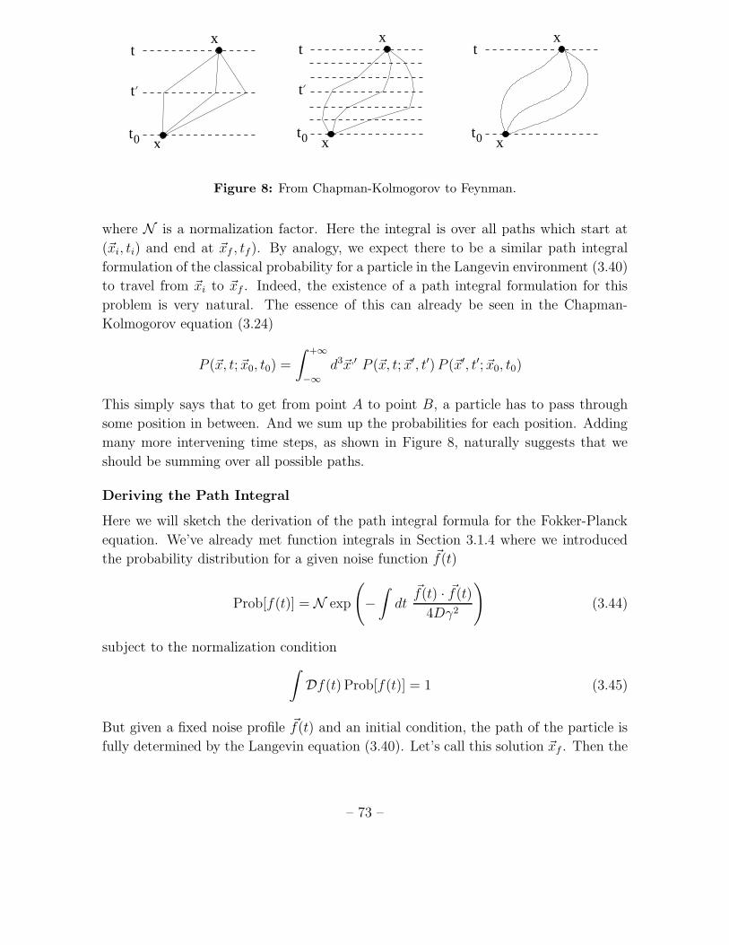
Figure 8: From Chapman-Kolmogorov to Feynman.

where N is a normalization factor. Here the integral is over all paths which start at

(~xi, ti) and end at ~xf , tf). By analogy, we expect there to be a similar path integral

formulation of the classical probability for a particle in the Langevin environment (3.40)

to travel from ~xi to ~xf . Indeed, the existence of a path integral formulation for this

problem is very natural. The essence of this can already be seen in the Chapman-

Kolmogorov equation (3.24)

P (~x, t; ~x0, t0) =

∫ +∞

−∞

d3~x,′ P (~x, t; ~x′, t′)P (~x′, t′; ~x0, t0)

This simply says that to get from point A to point B, a particle has to pass through

some position in between. And we sum up the probabilities for each position. Adding

many more intervening time steps, as shown in Figure 8, naturally suggests that we

should be summing over all possible paths.

Deriving the Path Integral

Here we will sketch the derivation of the path integral formula for the Fokker-Planck

equation. We’ve already met function integrals in Section 3.1.4 where we introduced

the probability distribution for a given noise function ~f(t)

Prob[f(t)] = N exp

(

−∫

dt~f(t) · ~f(t)

4Dγ2

)

(3.44)

subject to the normalization condition

∫

Df(t) Prob[f(t)] = 1 (3.45)

But given a fixed noise profile ~f(t) and an initial condition, the path of the particle is

fully determined by the Langevin equation (3.40). Let’s call this solution ~xf . Then the

– 73 –

probability that the particle takes the path ~xf is the same as the probability that the

force is ~f ,

Prob[~xf (t)] = Prob[~f(t)] = N exp

(

−∫

dt~f(t) · ~f(t)

4Dγ2

)

= N exp

(

− 1

4Dγ2

∫

dt (γ~xf + ∇V (~xf ))2

)

where, in the last line, we’ve used the Langevin equation (3.40) to relate the force to

the path taken. But since this equation holds for any path ~xf , we can simply drop the

f label. We have the probability that the particle takes a specific path ~x(t) given by

Prob[~x(t)] = N exp

(

− 1

4Dγ2

∫

dt (γ~x+ ∇V )2

)

The total probability to go from ~xi to ~xf should therefore just be the sum over all these

paths. With one, slightly fiddly, subtlety: the probability is normalized in (3.45) with

respect to the integration measure over noise variable ~f . And we want to integrate over

paths. This means that we have to change integration variables and pick up a Jacobian

factor for our troubles. We have

Prob[~xf , tf ; ~xi, ti] = N∫

Df(t) exp

(

− 1

4Dγ2

∫

dt (γ~xf + ∇V (~xf )2

)

= N∫

Dx(t) detM exp

(

− 1

4Dγ2

∫

dt (γ~x+ ∇V )2

)

(3.46)

Here the operator M(t, t′) that appears in the Jacobian be thought of as δf(t)/δx(t′).

It can be written down by returning to the Langevin equation (3.40) which relates fand

x,

M(t, t′) = γ∂

∂tδ(t− t′) + ∇2V δ(t− t′)

If we want to think in a simple minded way, we can consider this as a (very large)

matrix Mtt′ , with columns labelled by the index t and rows labelled by t′. We’ll write

the two terms in this matrix as M = A +B so the determinant becomes

det(A+B) = detA det(1 + A−1B) (3.47)

The first operator A = γ∂/∂t δ(t− t′) doesn’t depend on the path and its determinant

just gives a constant factor which can be absorbed into the normalization N . The

operator A−1 in the second term is defined in the usual way as∫

dt′A(t, t′)A−1(t,′ t′′) = δ(t− t′′)

– 74 –

where the integral over∫

dt′ is simply summing over the rows of A and the columns of

A−1 as in usual matrix multiplication. It is simple to check that the inverse is simply

the step function

A−1(t′, t′′) =1

γθ(t′ − t′′) (3.48)

Now we write the second factor in (3.47) and expand,

det(1 + A−1B) = exp(

Tr log(1 +A−1B))

= exp(

∑

n

Tr(A−1B)n/n)

(3.49)

Here we should look in more detail at what this compact notation means. The term

TrA−1B is really short-hand for

TrA−1B =

∫

dt dt′ A−t(t, t′)B(t′, t)

where the integral over∫

dt′ is multiplying the matrices together while the integral over∫

dt comes from taking the trace. Using (3.48) we have

TrA−1B =1

γ

∫

dt dt′ θ(t− t′)∇2V δ(t− t′) =θ(0)

γ

∫

dt ∇2V

The appearance of θ(0) may look a little odd. This function is defined to be θ(x) = +1

for x > 0 and θ(x) = 0 for x < 0. The only really sensible value at the origin is

θ(0) = 1/2. Indeed, this follows from the standard regularizations of the step function,

for example

θ(x) = limµ→0

(

1

2+

1

πtan−1

(

x

µ

))

⇒ θ(0) =1

2

What happens to the higher powers of (A−1B)n? Writing them out, we have

Tr(A−1B)n =

∫

dt

∫

dt1 . . . dt2n−1 θ(t− t1)δ(t1 − t2)θ(t2 − t3)δ(t3 − t4) . . .

. . . θ(t2n−2 − t2n−1)δ(t2n−1 − t)(∇2V )n

γn

where we have been a little sloppy in writing (∇2V )n because each of these is actually

computed at a different time. We can use the delta-functions to do half of the integrals,

say all the tn for n odd. We get

Tr(A−1B)n =

∫

dt

∫

dt2dt4 . . . θ(t− t2)θ(t2 − t4)θ(t4 − t6) . . . θ(t2n−2 − t)(∇2V )n

γn

– 75 –

But this integral is only non-vanishing only if t > t2 > t4 > t6 > . . . > tn > t. In

other words, the integral vanishes. (Note that you might think we could again get

contributions from θ(0) = 1/2, but the integrals now mean that the integrand has

support on a set of zero measure. And with no more delta-functions to rescue us, gives

zero. The upshot of this is that the determinant (3.49) can be expressed as a single

exponential

det(1 + A−1B) = exp

(

1

2γ

∫

dt ∇2V

)

We now have an expression for the measure factor in (3.46). Using this, the path

integral for the probability becomes,

Prob[~xf , tf ; ~xi, ti] = N ′

∫

Dx(t) exp

(

− 1

4Dγ2

∫

dt (γ~x+ ∇V )2 +1

2γ

∫

dt ∇2V

)

= N ′e[V (xf )−V (xi)]/2γD

∫

Dx(t) exp

(

−∫

dt~x 2

4D− U

)

where U is given in (3.43). Notice that the prefactor e[V (xf )−V (xi)]/2γD takes the same

form as the map from probabilities P to the rescaled P in (3.41). This completes our

derivation of the path integral formulation of probabilities.

3.2.5 Stochastic Calculus

There is one final generalization of the Langevin equation that we will mention but

won’t pursue in detail. Let’s return to the case m = 0, but generalise the noise term

in the Langevin equation so that it is now spatially dependent. We write

γ~x = −∇V + b(~x) ~f(t) (3.50)

This is usually called the non-linear Langevin equation. The addition of the b(~x) multi-

plying the noise looks like a fairly innocuous change. But it’s not. In fact, annoyingly,

this equation is not even well defined!

The problem is that the system gets a random kick at time t, the strength of which

depends on its position at time t. But if the system is getting a delta-function impulse

at time t then its position is not well defined. Mathematically, this problem arises when

we look at the position after some small time δt. Our equation (3.20) now becomes

δ~x = ~x δt = −1

γ∇V δt+

1

γ

∫ t+δt

t

dt′ b(~x(t′)) ~f(t′)

and our trouble is in making sense of the last term. There are a couple of obvious ways

we could move forward:

– 76 –

• Ito: We could insist that the strength of the kick is related to the position of the

particle immediately before the kick took place. Mathematically, we replace the

integral with

∫ t+δt

t

dt′ b(~x(t′)) ~f(t′) −→ b(~x(t))

∫ t+δt

t

dt′ ~f(t′)

This choice is known as Ito stochastic calculus.

• Stratonovich: Alternatively, we might argue that the kick isn’t really a delta

function. It is really a process that takes place over a small, but finite, time. To

model this, the strength of the kick should be determined by the average position

over which this process takes place. Mathematically, we replace the integral with,

∫ t+δt

t

dt′ b(~x(t′)) ~f(t′) −→ 1

2[b(~x(t+ δt)) + b(~x(t))]

∫ t+δt

t

dt′ ~f(t′)

This choice is known as Stratonovich stochastic calculus.

Usually in physics, issues of this kind don’t matter too much. Typically, any way of

regulating microscopic infinitesimals leads to the same macroscopic answers. However,

this is not the case here and the Ito and Stratonovich methods give different answers

in the continuum. In most applications of physics, including Brownian motion, the

Stratonovich calculus is the right way to proceed because, as we argued when we first

introduced noise, the delta-function arising in the correlation function 〈f(t)f(t′)〉 is just

a convenient approximation to something more smooth. However, in other applications

such as financial modelling, Ito calculus is correct.

The subject of stochastic calculus is a long one and won’t be described in this course9.

For the Stratonovich choice, the Fokker-Planck equation turns out to be

∂P

∂t=

1

γ∇ ·[

P (∇V −Dγ2b∇b)]

+D∇2(b2P )

This is also the form of the Fokker-Planck equation that you get by naively dividing

(3.50) by b(~x) and the defining a new variable ~y = ~x/b which reduces the problem to

our previous Langevin equation (3.19). In contrast, if we use Ito stochastic calculus,

the b∇b term is absent in the resulting Fokker-Planck equation.

9If you’d like to look at this topic further, there are a number of links to good lecture notes on the

course webpage.

– 77 –