3D G-CNNs for Pulmonary Nodule Detection

Marysia WinkelsUniversity of Amsterdam / Aidence

marysia@aidence.com

Taco S. CohenUniversity of Amsterdamtaco.cohen@gmail.com

Abstract

Convolutional Neural Networks (CNNs) require a large amount of annotated datato learn from, which is often difficult to obtain in the medical domain. In thispaper we show that the sample complexity of CNNs can be significantly improvedby using 3D roto-translation group convolutions (G-Convs) instead of the moreconventional translational convolutions. These 3D G-CNNs were applied to theproblem of false positive reduction for pulmonary nodule detection, and proved tobe substantially more effective in terms of performance, sensitivity to malignantnodules, and speed of convergence compared to a strong and comparable baselinearchitecture with regular convolutions, data augmentation and a similar number ofparameters. For every dataset size tested, the G-CNN achieved a FROC score closeto the CNN trained on ten times more data.

1 Introduction

Lung cancer is currently the leading cause of cancer-related death worldwide, accounting for anestimated 1.7 million deaths globally each year and 270,000 in the European Union alone [1, 2],taking more victims than breast cancer, colon cancer and prostate cancer combined [3]. This highmortality rate can be largely attributed to the fact that the majority of lung cancer is diagnosed whenthe cancer has already metastasised as symptoms generally do not present themselves until the canceris at a late stage, making early detection difficult [4].

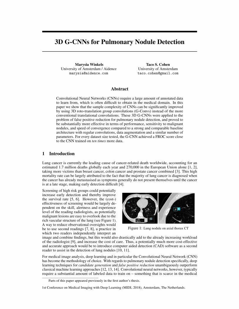
Figure 1: Lung nodule on axial thorax CT

Screening of high risk groups could potentiallyincrease early detection and thereby improvethe survival rate [5, 6]. However, the (cost-)effectiveness of screening would be largely de-pendent on the skill, alertness and experiencelevel of the reading radiologists, as potentiallymalignant lesions are easy to overlook due to therich vascular structure of the lung (see Figure 1).A way to reduce observational oversights wouldbe to use second readings [7, 8], a practice inwhich two readers independently interpret animage and combine findings, but this would also drastically add to the already increasing workloadof the radiologist [9], and increase the cost of care. Thus, a potentially much more cost-effectiveand accurate approach would be to introduce computer aided detection (CAD) software as a secondreader to assist in the detection of lung nodules [10, 11].

For medical image analysis, deep learning and in particular the Convolutional Neural Network (CNN)has become the methodology of choice. With regards to pulmonary nodule detection specifically, deeplearning techniques for candidate generation and false positive reduction unambiguously outperformclassical machine learning approaches [12, 13, 14]. Convolutional neural networks, however, typicallyrequire a substantial amount of labeled data to train on – something that is scarce in the medical

Parts of this paper appeared previously in the first author’s thesis.

1st Conference on Medical Imaging with Deep Learning (MIDL 2018), Amsterdam, The Netherlands.

imaging community, both due to patient privacy concerns and the labor-intensity of obtaining high-quality annotations. The problem is further compounded by the fact that in all likelihood, manyCAD systems will have to be developed for different imaging modalities, scanner types, settings,resolutions, and patient populations. All of this suggests that data efficiency is a major hurdle to thescalable development of CAD systems such as those which are the focus of the current work: lungnodule detection systems.

Relative to fully connected networks, CNNs are already more data efficient. This is due to thetranslational weight sharing in the convolutional layers. One important property of convolution layersthat enables translational weight sharing, but is rarely discussed explicitly, is translation equivariance:a shift in the input of a layer leads to a shift in the output, f(Tx) = Tf(x). Because each layer ina CNN is translation equivariant, all internal representations will shift when the network input isshifted, so that translational weight sharing is effective in each layer of a deep network.

Many kinds of patterns, including pulmonary nodules, maintain their identity not just under translation,but also under other transformations such as rotation and reflection. So it is natural to ask if CNNscan be generalized to other kinds of transformations, and indeed it was shown that by using groupconvolutions, weight sharing and equivariance can be generalized to essentially arbitrary groups oftransformations [15]. Although the general theory of G-CNNs is now well established [15, 16, 17, 18],a lot of work remains in developing easy to use group convolution layers for various kinds of inputdata with various kinds of symmetries. This is a burgeoning field of research, with G-CNNs beingdeveloped for discrete 2D rotation and reflection symmetries [15, 19, 16], continuous planar rotations[20, 21, 22], 3D rotations of spherical signals [23], and permutations of nodes in a graph [24].

In this paper, we develop G-CNNs for three-dimensional signals such as volumetric CT images, actedon by discrete translations, rotations, and reflections. This is highly non-trivial, because the discreteroto-reflection groups in three dimensions are non-commutative and have a highly intricate structure(see Figure 3). We show that when applied to the task of false-positive reduction for pulmonarynodule detection in chest CT scans, 3D G-CNNs show remarkable data efficiency, yielding similarperformance to CNNs trained on 10× more data. Our implementation of 3D group convolutions ispublicly available1, so that using them is as easy as replacing Conv3D() by GConv3D().

In what follows, we will provide a high-level overview of group convolutions as well as the various3D roto-reflection groups considered in this work (section 2). Section 3 describes the experimentalsetup, including datasets, evaluation protocol network architectures, and section 4 compares G-CNNsto conventional CNNs in terms of performance and rate of convergence. We discuss these results andconclude in sections 5 and 6 respectively.

2 Three-dimensional G-CNNs

In this section we will explain the 3D group convolution in an elementary fashion. The goal isto convey the high level idea, focusing on the algorithm rather than the underlying mathematicaltheory, and using visual aids where this is helpful. For the general theory, we refer the reader to[15, 16, 17, 18].

To compute the conventional (translational) convolution of a filter with a feature map, the filteris translated across the feature map, and a dot product is computed at each position. Each cellof the output feature map is thus associated with a translation that was applied to the filter. In agroup convolution, additional transformations like rotations and reflections are applied to the filters,thereby increasing the degree of weight sharing. More specifically, starting with a canonical filterwith learnable parameters, one produces a number of transformed copies, which are then convolved(translationally) with the input feature maps to produce a set of output feature maps.

Thus, each learnable filter produces a number of orientation channels, each of which detects the samefeature in a different orientation. We will refer to the set of orientation channels associated with onefeature / filter as one feature map.

As shown in [15], if the transformations that are applied to the filters are chosen to form a symmetrygroup H (more on that later), the resulting feature maps will be equivariant to transformations fromthis group (as well as being equivariant to translations). More specifically, if we transform the input

1https://github.com/tscohen/GrouPy

2

by h ∈ H (e.g. rotate it by 90 degrees), each orientation channel will be transformed by h in thesame way, and the orientation channels will get shuffled by a permutation matrix ρ(h).

The channel-shuffling phenomenon occurs because the transformation h changes the orientation ofthe input pattern, so that it gets picked up by a different orientation channel / transformed filter. Theparticular way in which the channels get shuffled by each element h ∈ H depends on the structure ofH (i.e. the way transformations g, k ∈ H compose to form a third transformation h = gk ∈ H), andis the subject of subsection 2.1.

Because of the output feature maps of a G-Conv layer have orientation channels, the filters in thesecond and higher layers will also need orientation channels to match those of the input. Furthermore,when applying a transformation h ∈ H to a filter that has orientation channels, we must also shufflethe orientation channels of the filter. Doing so, the feature maps of the next layer will again haveorientation channels that jointly transform equivariantly with the input of the network, so we canstack as many of these layers as we like while maintaining equivariance of the network.

In the simplest instantiation of G-CNNs, the group H is the set of 2D planar rotations by 0, 90, 180and 270 degrees, and the whole group G is just H plus 2D translations. In this case, there are fourorientation channels per feature, which undergo a cyclic permutation under rotation. In 3D, however,things get substantially more complicated. In the following section, we will discuss the various 3Droto-reflection groups considered in this paper, and show how one may derive the channel shufflingpermutation ρ(h) for each symmetry transformation h. Then, in section 2.2, we provide a detaileddiscussion of the implementation of 3D group convolutions.

2.1 3D roto-reflection groups

In general, the symmetry group of an object is the set of transformations that map that object back ontoitself without changing it. For instance, a square can be rotated by 0, 90, 180 and 270 degrees, andflipped, without changing it. The set of symmetries of an object has several obvious properties, such asclosure (the composition gh of two symmetries g and h is a symmetry), associativity (h(gk) = (hg)kfor transformations h, g and k), identity (the identity map is always a symmetry), and inverses (theinverse of a symmetry is always a symmetry). These properties can be codified as axioms and studiedabstractly, but in this paper we will only study concrete symmetry groups that are of use in 3DG-CNNs, noting only that all ideas in this paper are easily generalized to a wide variety of settings bymoving to a more abstract level.

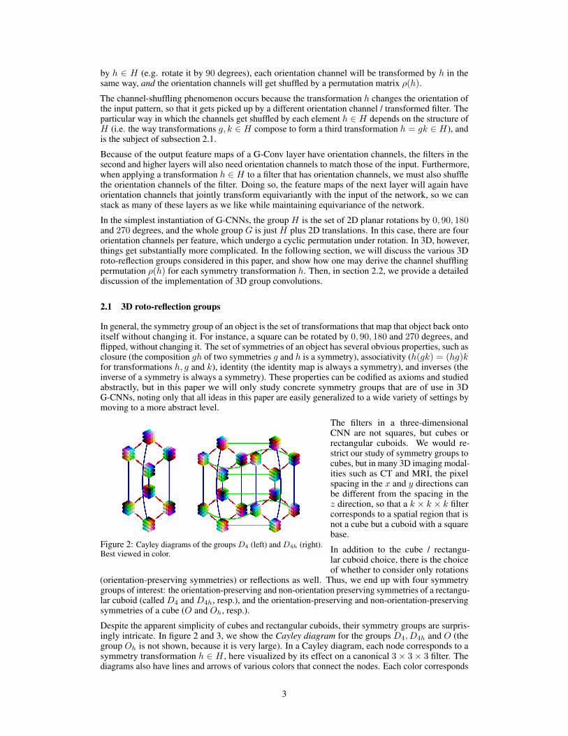
Figure 2: Cayley diagrams of the groups D4 (left) and D4h (right).Best viewed in color.

The filters in a three-dimensionalCNN are not squares, but cubes orrectangular cuboids. We would re-strict our study of symmetry groups tocubes, but in many 3D imaging modal-ities such as CT and MRI, the pixelspacing in the x and y directions canbe different from the spacing in thez direction, so that a k × k × k filtercorresponds to a spatial region that isnot a cube but a cuboid with a squarebase.

In addition to the cube / rectangu-lar cuboid choice, there is the choiceof whether to consider only rotations

(orientation-preserving symmetries) or reflections as well. Thus, we end up with four symmetrygroups of interest: the orientation-preserving and non-orientation preserving symmetries of a rectangu-lar cuboid (called D4 and D4h, resp.), and the orientation-preserving and non-orientation-preservingsymmetries of a cube (O and Oh, resp.).

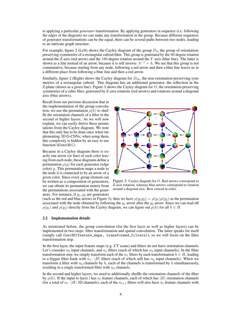
Despite the apparent simplicity of cubes and rectangular cuboids, their symmetry groups are surpris-ingly intricate. In figure 2 and 3, we show the Cayley diagram for the groups D4, D4h and O (thegroup Oh is not shown, because it is very large). In a Cayley diagram, each node corresponds to asymmetry transformation h ∈ H , here visualized by its effect on a canonical 3× 3× 3 filter. Thediagrams also have lines and arrows of various colors that connect the nodes. Each color corresponds

3

to applying a particular generator transformation. By applying generators in sequence (i.e. followingthe edges of the diagram) we can make any transformation in the group. Because different sequencesof generator transformations can be the equal, there can be several paths between two nodes, leadingto an intricate graph structure.

For example, figure 2 (Left) shows the Cayley diagram of the group D4, the group of orientation-preserving symmetries of a rectangular cuboid filter. This group is generated by the 90-degree rotationaround the Z-axis (red arrow) and the 180-degree rotation around the Y -axis (blue line). The latter isshown as a line instead of an arrow, because it is self inverse: h−1 = h. We see that this group is notcommutative, because starting from any node, following a red arrow and then a blue line leaves us ina different place from following a blue line and then a red arrow.

Similarly, figure 2 (Right) shows the Cayley diagram for D4h, the non-orientation-preserving sym-metries of a rectangular cuboid. This diagram has an additional generator, the reflection in theZ-plane (drawn as a green line). Figure 3 shows the Cayley diagram for O, the orientation-preservingsymmetries of a cubic filter, generated by Z-axis rotations (red arrows) and rotations around a diagonalaxis (blue arrows).

Figure 3: Cayley diagram for O. Red arrows correspond toZ-axis rotation, whereas blue arrows correspond to rotationaround a diagonal axis. Best viewed in color.

Recall from our previous discussion that inthe implementation of the group convolu-tion, we use the permutation ρ(h) to shuf-fle the orientation channels of a filter in thesecond or higher layers. As we will nowexplain, we can easily derive these permu-tations from the Cayley diagram. We notethat this only has to be done once when im-plementing 3D G-CNNs; when using them,this complexity is hidden by an easy to usefunction GConv3D().

Because in a Cayley diagram there is ex-actly one arrow (or line) of each color leav-ing from each node, these diagrams define apermutation ρ(g) for each generator (edgecolor) g. This permutation maps a node tothe node it is connected to by an arrow of agiven color. Since every group element canbe written as a composition of generators,we can obtain its permutation matrix fromthe permutations associated with the gener-ators. For instance, if g1, g2 are generators(such as the red and blue arrows in Figure 3), then we have ρ(g1g2) = ρ(g1)ρ(g2) as the permutationassociated with the node obtained by following the g1 arrow after the g2 arrow. Since we can read offρ(g1) and ρ(g2) directly from the Cayley diagram, we can figure out ρ(h) for all h ∈ H .

2.2 Implementation details

As mentioned before, the group convolution (for the first layer as well as higher layers) can beimplemented in two steps: filter transformation and spatial convolution. The latter speaks for itself(simply call Conv3D(feature_maps, transformed_filters)), so we will focus on the filtertransformation step.

In the first layer, the input feature maps (e.g. CT scans) and filters do not have orientation channels.Let’s consider n0 input channels, and n1 filters (each of which has n0 input channels). In the filtertransformation step, we simply transform each of the n1 filters by each transformation h ∈ H , leadingto a bigger filter bank with n1 · |H| filters (each of which still has n0 input channels). When wetransform a filter with n0 channels by h, each of the channels is transformed by h simultaneously,resulting in a single transformed filter with n0 channels.

In the second and higher layers, we need to additionally shuffle the orientation channels of the filterby ρ(h). If the input to layer l has nl feature channels, each of which has |H| orientation channels(for a total of nl · |H| 3D channels), each of the nl+1 filters will also have nl feature channels with

4

|H| orientation channels each. During the filter transformation step, the filters again get transformedby each element h ∈ H , so that we end up with nl+1 · |H| transformed filters, and equally many 3Doutput channels.

Since the discrete rotations and reflections of a filter will spatially permute the pixels, and ρ(h)permutes channels, the whole filter transformation is just the application of |H| permutations tothe filter bank. This can easily be implemented by an indexing operation of the filter bank with aprecomputed set of indices, or by multiplying by a precomputed permutation matrix. For the detailsof how to precompute these, we refer to our implementation.

Considering that the cost of the filter transformation is negligible, the computational cost of a groupconvolution is roughly equal to the computational cost of a regular spatial convolution with a filterbank whose size is equal to the augmented filter bank used in the group convolution. In practice, wetypically reduce the number of feature maps in a G-CNN, to keep the amount of computation thesame, or to keep the number of parameters the same.

3 Experiments

Modern pulmonary nodule detection systems consist of the following five subsystems: data acquisition(obtaining the medical images), preprocessing (to improve image quality), segmentation (to separatelung tissue from other organs and tissues on the chest CT), localisation (detecting suspect lesions andpotential nodule candidates) and false positive reduction (classification of found nodule candidates asnodule or non-nodule). The experiments in this work will focus on false positive reduction only. Thisreduces the problem to a relatively straightforward classification problem, and thus enables a cleancomparison between CNNs and G-CNNs, evaluated under identical circumstances.

To determine whether a G-CNN is indeed beneficial for false positive reduction, the performanceof networks with G-Convs for various 3D groups G (see subsection 2.1) are compared to a baselinenetwork with regular 3D convolutions. To further investigate the data-efficiency of CNNs and G-CNNs, we conduct this experiment for various training dataset sizes varying from 30 to 30,000 datasamples. In addition, we evaluated the convergence speed of G-CNNs and regular CNNs, and foundthat the former converge substantially faster.

3.1 Datasets

The scans used for the experiments originate from the NLST [5] and LIDC/IDRI [25] datasets. TheNLST dataset contains scans from the CT arm of the National Lung Screening Trial, a randomizedcontrolled trial to determine whether screening with low-dose CT (without contrast) reduces themortality from lung cancer in high-risk individuals relative to screening with chest radiography. TheLIDC/IDRI dataset is relatively varied, as scans were acquired with a wide range of scanner modelsand acquisition parameters and contains both low-dose and full-dose CTs taken with or withoutcontrast. The images in the LIDC/IDRI database were combined with nodule annotations as well assubjective assessments of various nodule characteristics (such as suspected malignancy) provided byfour expert thoracic radiologists. Unlike the NLST, the LIDC/IDRI database does not represent ascreening population, as the inclusion criteria allowed any type of participant.

All scans from the NLST and LIDC/IDRI datasets with an original slice thickness equal to or lessthan 2.5mm were processed by the same candidate generation model to provide center coordinatesof potential nodules. These center coordinates were used to extract 12× 72× 72 patches from theoriginal scans, where each voxel represents 1.25× .5× .5mm of lung tissue. Values of interest fornodule detection lie approximately between -1000 Hounsfield Units (air) and 300 Hounsfield Units(soft-tissue) and this range was normalized to a [−1, 1] range.

Due to the higher annotation quality and higher variety of acquisition types of the LIDC/IDRI, alongwith the higher volume of available NLST image data, the training and validation is done on potentialcandidates from the NLST dataset and testing is done on the LIDC/IDRI nodule candidates. Thisdivision of datasets, along with the exclusion of scans with a slice thickness greater than 2.5mm,allowed us to use the reference standard for nodule detection as used by the LUNA16 grand challenge[26] and performance metric as specified by the ANODE09 study [27]. This setup results in a totalof 30, 000 data samples for training, 8, 889 for validation, and 8, 582 for testing. Models are trainedon subsets of this dataset of various sizes: 30, 300, 3,000 and 30,000 samples. Each training set is

5

Set Source Candidates Positive % Negative %Training NLST max. 30,000 50.0 50.0Validation NLST 8,889 20.6 79.4Test LIDC/IDRI 8,582 13.3 86.7Table 1: Specifics of the training, validation and test set sizes and class ratios.

balanced, and each smaller training set is a subset of all larger training sets. The details of the train,validation and test sets are specified in Table 1.

3.2 Network architectures & training procedure

A baseline network was established with 6 convolutional layers consisting of 3× 3× 3 convolutions,batch normalization and ReLU nonlinearities. In addition, the network uses 3D max pooling withsame padding after the first, third and fifth layer, dropout after the second and fourth layer, and hasa fully-connected layer as a last layer. We refer to this baseline network as the Z3-CNN, because,like every conventional 3D CNN, it is a G-CNN for the group of 3D translations, Z3. The Z3-CNNbaseline, when trained on the whole dataset, was found to achieve competitive performance basedon the LUNA16 grand challenge leader board, and therefore deemed sufficiently representative of amodern pulmonary nodule CAD system.

The G-Conv variants of the baseline were created by simply replacing the 3D convolution in thebaseline with a G-Conv for the group D4, D4h, O or Oh (see section 2.1). This leads to an increasein the number of 3D channels, and hence the number of parameters per filter. Hence, the number ofdesired output channels (nl+1) is divided by

√|H| to keep the number of parameters roughly the

same and the network comparable to the baseline.

We minimize the cross-entropy loss using the Adam optimizer [28]. The weights were initializedusing the uniform Xavier method [29]. For training, we use a mini-batch size of 30 (the size of thesmallest training set) for all training set sizes. We use validation-based early stopping. A single dataaugmentation scheme (continuous rotation by 0− 360o, reflection over all axes, small translationsover all axes, scaling between .8− 1.2, added noise, value remapping) was used for all training runsand all architectures.

3.3 Evaluation

Despite the availability of a clear definition of a lung nodule (given by the Fleischer Glossary), severalstudies confirm that observers often disagree on what constitutes a lung nodule [30, 31, 32]. Thisposes a problem in the benchmarking of CAD systems.

In order to deal with inter-observer disagreements, only those nodules accepted by 3 out of fourradiologists (and ≥ 3mm and ≤ 30mm in largest axial diameter) are considered essential for thesystem to detect. Nodules accepted by fewer than three radiologists, those smaller than 3mm or largerthan 30mm in diameter, or with benign characteristics such as calcification, are ignored in evaluationand do not count towards the positives or the negatives. The idea to differentiate between relevant(essential to detect) and irrelevant (optional to detect) findings was first proposed in the ANODE09study [27].

ANODE09 also introduced the Free-Response Operating Characteristic (FROC) analysis, wherethe sensitivity is plotted against the average number of false positives per scan. FROC analysis,as opposed to any single scalar performance metric, makes it possible to deal with differences inpreference regarding the trade-off between sensitivity and false positive rate for various users. We usethis to evaluate our systems. To also facilitate direct quantitative comparisons between systems, wecompute an overall system score based on the FROC analysis, which is the average of the sensitivityat seven predefined false positive rates ( 18 ;

14 ;

12 ; 1; 2; 4; and 8).

This evaluation protocol described in this section is identical to the method used to score theparticipants of the LUNA16 nodule detection grand challenge [26], and is the de facto standard forevaluation of lung nodule detection systems.

6

4 Results

4.1 FROC analysis

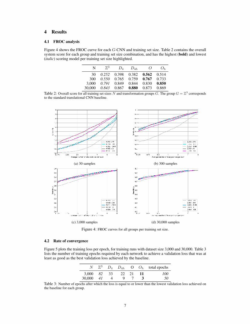
Figure 4 shows the FROC curve for each G-CNN and training set size. Table 2 contains the overallsystem score for each group and training set size combination, and has the highest (bold) and lowest(italic) scoring model per training set size highlighted.

N Z3 D4 D4h O Oh

30 0.252 0.398 0.382 0.562 0.514300 0.550 0.765 0.759 0.767 0.733

3,000 0.791 0.849 0.844 0.830 0.85030,000 0.843 0.867 0.880 0.873 0.869

Table 2: Overall score for all training set sizes N and transformation groups G. The group G = Z3 correspondsto the standard translational CNN baseline.

(a) 30 samples (b) 300 samples

(c) 3,000 samples (d) 30,000 samples

Figure 4: FROC curves for all groups per training set size.

4.2 Rate of convergence

Figure 5 plots the training loss per epoch, for training runs with dataset size 3,000 and 30,000. Table 3lists the number of training epochs required by each network to achieve a validation loss that was atleast as good as the best validation loss achieved by the baseline.

N Z3 D4 D4h O Oh total epochs

3,000 82 33 22 21 11 10030,000 41 4 9 7 3 50

Table 3: Number of epochs after which the loss is equal to or lower than the lowest validation loss achieved onthe baseline for each group.

7

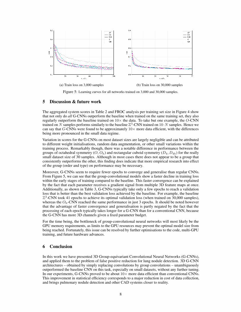
(a) Train loss on 3,000 samples (b) Train loss on 30,000 samples

Figure 5: Learning curves for all networks trained on 3,000 and 30,000 samples.

5 Discussion & future work

The aggregated system scores in Table 2 and FROC analysis per training set size in Figure 4 showthat not only do all G-CNNs outperform the baseline when trained on the same training set, they alsoregularly outperform the baseline trained on 10× the data. To take but one example, the O-CNNtrained onN samples performs similarly to the baseline Z3-CNN trained on 10·N samples. Hence wecan say that G-CNNs were found to be approximately 10× more data efficient, with the differencesbeing more pronounced in the small data regime.

Variation in scores for the G-CNNs on most dataset sizes are largely negligible and can be attributedto different weight initialisations, random data augmentation, or other small variations within thetraining process. Remarkably though, there was a notable difference in performance between thegroups of octahedral symmetry (O, Oh) and rectangular cuboid symmetry (D4, D4h) for the reallysmall dataset size of 30 samples. Although in most cases there does not appear to be a group thatconsistently outperforms the other, this finding does indicate that more empirical research into effectof the group (order and type) on performance may be necessary.

Moreover, G-CNNs seem to require fewer epochs to converge and generalise than regular CNNs.From Figure 5, we can see that the group-convolutional models show a faster decline in training losswithin the early stages of training compared to the baseline. This faster convergence can be explainedby the fact that each parameter receives a gradient signal from multiple 3D feature maps at once.Additionally, as shown in Table 3, G-CNNs typically take only a few epochs to reach a validationloss that is better than the best validation loss achieved by the baseline. For example, the baselineZ3-CNN took 41 epochs to achieve its optimal validation loss (when trained on 30,000 samples),whereas the Oh-CNN reached the same performance in just 3 epochs. It should be noted howeverthat the advantage of faster convergence and generalisation is partly negated by the fact that theprocessing of each epoch typically takes longer for a G-CNN than for a conventional CNN, becausethe G-CNN has more 3D channels given a fixed parameter budget.

For the time being, the bottleneck of group-convolutional neural networks will most likely be theGPU memory requirements, as limits to the GPU resources may prevent the optimal model size frombeing reached. Fortunately, this issue can be resolved by further optimisations to the code, multi-GPUtraining, and future hardware advances.

6 Conclusion

In this work we have presented 3D Group-equivariant Convolutional Neural Networks (G-CNNs),and applied them to the problem of false positive reduction for lung nodule detection. 3D G-CNNarchitectures – obtained by simply replacing convolutions by group convolutions – unambiguouslyoutperformed the baseline CNN on this task, especially on small datasets, without any further tuning.In our experiments, G-CNNs proved to be about 10× more data efficient than conventional CNNs.This improvement in statistical efficiency corresponds to a major reduction in cost of data collection,and brings pulmonary nodule detection and other CAD systems closer to reality.

8

References[1] H. Wang et al. Global, regional, and national life expectancy, all-cause mortality, and cause-

specific mortality for 249 causes of death, 1980–2015: a systematic analysis for the GlobalBurden of Disease Study 2015. Lancet, 388:1459–1544, October 2016. doi:10.1016/S0140-6736(16)31012-1. PMID 27733281.

[2] Eurostat. Health in the European Union – facts and figures, September 2017.Data extracted in September 2017. Planned article update: January 2019. Avail-able at http://ec.europa.eu/eurostat/statistics-explained/index.php/Cancer_statistics_-_specific_cancersLung_cancer.

[3] American Cancer Society Cancer Statistics Center. Lung Cancer key statistics. Last update:January 2017. Available at https://www.cancer.org/cancer/non-small-cell-lung-cancer/about/key-statistics.html.

[4] American Cancer Society. Lung Cancer Detection and Early Prevention. Last revised: Febru-ary 22, 2016. Available at https://www.cancer.org/cancer/lung-cancer/prevention-and-early-detection/early-detection.html.

[5] The National Lung Screening Trial Research Team. Reduced Lung-Cancer Mortality with Low-Dose Computed Tomographic Screening. New England Journal of Medicine, 365(5):395–409,2011. PMID: 21714641.

[6] M. Oudkerk et al. European position statement on lung cancer screening. The Lancet Oncology,18:754–766, November 2017.

[7] P.M. Lauritzen et al. Radiologist-initiated double reading of abdominal CT: retrospectiveanalysis of the clinical importance of changes to radiology reports. BMJ quality & safety,25(8):595–603, August 2016.

[8] D. Wormanns; K. Ludwig; F. Beyer; W. Heindel; S. Diederich. Detection of pulmonary nodulesat multirow-detector CT: effectiveness of double reading to improve sensitivity at standard-doseand low-dose chest CT. European Journal of Radiology, 15(1):14–22, January 2005.

[9] J.H. Sunshine M. Bhargavan; A.H. Kaye; H.P. Forman. Workload of radiologists in UnitedStates in 2006-2007 and trends since 1991-1992. Radiology, 252(2):458–467, August 2009.

[10] L. Bogoni; J.P. Ko; J. Alpert J et al. Impact of a computer-aided detection (CAD) systemintegrated into a picture archiving and communication system (PACS) on reader sensitivity andefficiency for the detection of lung nodules in thoracic CT exams. J Digit Imaging, 25(6), 2012.

[11] Y. Zhao et al. Performance of computer-aided detection of pulmonary nodules in low-doseCT: comparison with double reading by nodule volume. European radiology, 22(10):2076–84,October 2012.

[12] B. van Ginneken. Fifty years of computer analysis in chest imaging: rule-based, machinelearning, deep learning. Radiological Physics and Technology, 10(2), February 2017.

[13] M. Firmino; A.H. Morais; R.M. Mendoca; M.R. Dantas; H.R. Hekis; R. Valentim. Computer-aided detection system for lung cancer in computed tomography scans: review and futureprospects. Biomed Eng Online, 13(1), 2014.

[14] B. Al Mohammad; P.C. Brennan; C. Mello-Thoms. A review of lung cancer screening and therole of computer-aided detection. Clinical Radiology, 72(1):433–442, January 2017.

[15] T.S. Cohen; M. Welling. Group equivariant convolutional networks. In International Conferenceon Machine Learning, pages 2990–2999, 2016.

[16] T.S. Cohen; M. Welling. Steerable CNNs. In International Conference on Learning Representa-tions, 2017.

[17] R. Kondor; S. Trivedi. On the Generalization of Equivariance and Convolution in NeuralNetworks to the Action of Compact Groups. 2018.

9

[18] T. S. Cohen; M. Geiger; M. Weiler. Intertwiners between Induced Representations (withApplications to the Theory of Equivariant Neural Networks. 2018.

[19] S. Dieleman; J. D. Fauw; K. Kavukcuoglu. Exploiting cyclic symmetry in convolutional neuralnetworks. International Conference on Machine Learning, page 1889–1898, June 2016.

[20] D. E. Worrall; S. J. Garbin; D. Turmukhambetov; G. J. Brostow. Harmonic Networks: DeepTranslation and Rotation Equivariance. In The IEEE Conference on Computer Vision andPattern Recognition (CVPR), 2017.

[21] M. Weiler; F. A. Hamprecht; M. Storath. Learning Steerable Filters for Rotation EquivariantCNNs. In The IEEE Conference on Computer Vision and Pattern Recognition (CVPR), 2018.

[22] Maxime W; Veta Mitko; Eppenhof Koen A J; Pluim Josien P W Bekkers, Erik J; Lafarge.Roto-Translation Covariant Convolutional Networks for Medical Image Analysis. April 2018.

[23] T.S. Cohen; M. Geiger; J. Koehler; M. Welling. Spherical CNNs. In International Conferenceon Learning Representations (ICLR), 2018.

[24] R. Kondor; H.T. Son; H. Pan; B. Anderson; S. Trivedi. Covariant Compositional Networks ForLearning Graphs. January 2018.

[25] M.F. McNitt-Gray; S.G. Armato; C.R. Meyer; A.P. Reeves; G. McLennan; R.C. Pais; J.Freymann; M.S. Brown; R.M. Engelmann; P.H. Bland; G.E. Laderach; C. Piker; J. Guo; Z.Towfic; D.P.Y. Qing; D.F. Yankelevitz; D.R. Aberle; E.J.R. van Beek; H. MacMahon; E.A.Kazerooni; B.Y. Croft; L.P. Clarke. The Lung Image Database Consortium (LIDC) DataCollection Process for Nodule Detection and Annotation. Radiology, 14(12):1464–1474,December 2007.

[26] A.A.A. Setio et al. Validation, comparison, and combination of algorithms for automaticdetection of pulmonary nodules in computed tomography images: the LUNA16 challenge.CoRR, abs/1612.08012, 2016.

[27] Bram Van Ginneken, Samuel G Armato, Bartjan de Hoop, Saskia van Amelsvoort-van deVorst, Thomas Duindam, Meindert Niemeijer, Keelin Murphy, Arnold Schilham, AlessandraRetico, Maria Evelina Fantacci, et al. Comparing and combining algorithms for computer-aideddetection of pulmonary nodules in computed tomography scans: the anode09 study. Medicalimage analysis, 14(6):707–722, 2010.

[28] D.P. Kingma; J. Ba. Adam: A Method for Stochastic Optimization. CoRR, 2014.

[29] X. Glorot; Y. Bengio. Understanding the difficulty of training deep feedforward neural networks.International Conference on Artificial Intelligence and Statistics, pages 249–256, 2010.

[30] Geoffrey D Rubin, John K Lyo, David S Paik, Anthony J Sherbondy, Lawrence C Chow,Ann N Leung, Robert Mindelzun, Pamela K Schraedley-Desmond, Steven E Zinck, David PNaidich, et al. Pulmonary nodules on multi–detector row CT scans: performance comparisonof radiologists and computer-aided detection. Radiology, 234(1):274–283, 2005.

[31] S. G. Armato et al. The Lung Image Database Consortium (LIDC): an evaluation of radiologistvariability in the identification of lung nodules on CT scans. Academic radiology, 14(11):1409–21, November 2007.

[32] Samuel G Armato, Rachael Y Roberts, Masha Kocherginsky, Denise R Aberle, Ella A Kazerooni,Heber MacMahon, Edwin JR van Beek, David Yankelevitz, Geoffrey McLennan, Michael FMcNitt-Gray, et al. Assessment of radiologist performance in the detection of lung nodules:dependence on the definition of “truth”. Academic radiology, 16(1):28–38, 2009.

10

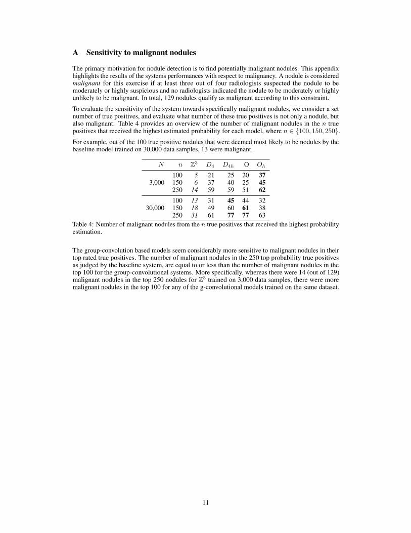
A Sensitivity to malignant nodules

The primary motivation for nodule detection is to find potentially malignant nodules. This appendixhighlights the results of the systems performances with respect to malignancy. A nodule is consideredmalignant for this exercise if at least three out of four radiologists suspected the nodule to bemoderately or highly suspicious and no radiologists indicated the nodule to be moderately or highlyunlikely to be malignant. In total, 129 nodules qualify as malignant according to this constraint.

To evaluate the sensitivity of the system towards specifically malignant nodules, we consider a setnumber of true positives, and evaluate what number of these true positives is not only a nodule, butalso malignant. Table 4 provides an overview of the number of malignant nodules in the n truepositives that received the highest estimated probability for each model, where n ∈ {100, 150, 250}.For example, out of the 100 true positive nodules that were deemed most likely to be nodules by thebaseline model trained on 30,000 data samples, 13 were malignant.

N n Z3 D4 D4h O Oh

100 5 21 25 20 373,000 150 6 37 40 25 45

250 14 59 59 51 62100 13 31 45 44 32

30,000 150 18 49 60 61 38250 31 61 77 77 63

Table 4: Number of malignant nodules from the n true positives that received the highest probabilityestimation.

The group-convolution based models seem considerably more sensitive to malignant nodules in theirtop rated true positives. The number of malignant nodules in the 250 top probability true positivesas judged by the baseline system, are equal to or less than the number of malignant nodules in thetop 100 for the group-convolutional systems. More specifically, whereas there were 14 (out of 129)malignant nodules in the top 250 nodules for Z3 trained on 3,000 data samples, there were moremalignant nodules in the top 100 for any of the g-convolutional models trained on the same dataset.

11