Embed Size (px)
Citation preview
3D Numerical Modelling of Secondary Current in Shallow River
Bends and Confluences
By
Rawaa Shaheed
A thesis submitted under supervisions of
Dr. Majid Mohammadian
in partial fulfilment of the requirements for the degree of
Masters of Applied Science in Civil Engineering
Department of Civil Engineering
University of Ottawa
Ottawa, Canada
May 2016
The M.A.Sc. in Civil Engineering is a joint program
with Carleton University administrated
by Ottawa-Carleton Institute for Civil Engineering
© Rawaa Shaheed, Ottawa, Canada, 2016
ii
))وما توفيقي الا ابهلل عليه تولكت واليه انيب((
" and my success can only come from Allah. In Him
I trust, and unto Him I return." [Hud:88]

iii
To...
The spirit of my parents ...
My Lovely Husband...
Brother, Sisters...and all My Family...
With my Love...
iv
Abstract
Secondary currents are one of the important features that characterize flow in river bends and
confluences. Fluid particles follow a helical path instead of moving nearly parallel to the axis
of the channel. The local imbalance between the vertically varying centrifugal force and the
cross-stream pressure gradient results in generating the secondary flow and raising a typical
motion of the helical flow. A number of studies, including experimental or mathematical, have
been conducted to examine flow characteristics in curved open channels, river meanders, or
confluences. In this research, the influence of secondary currents is studied on the elevation
of water surface and the hydraulic structures in channel bends and confluences by employing
a 3D OpenFOAM numerical model.
The research implements the 3D OpenFOAM numerical model to simulate the horizontal
distribution of the flow in curved rivers. In addition, the progress in unraveling and
understanding the bend dynamics is considered. The finite volume method in (OpenFOAM)
software is used to simulate and examine the behavior of secondary current in channel bends
and confluences. Thereafter, a comparison between the experimental data and a numerical
model is conducted. Two sets of experimental data are used; the data provided by Rozovskii
(1961) for sharply curved channel, and the dataset provided by Shumate (1998) for confluent
channel.
Two solvers in (OpenFOAM) software were selected to solve the problem regarding the
experiment; InterFoam and PisoFoam. The InterFoam is a transient solver for incompressible
flow that is used with open channel flow and Free Surface Model. The PisoFoam is a transient
solver for incompressible flow that is used with closed channel flow and Rigid-Lid Model.
Various turbulence models (i.e. Standard k-ε, Realizable k-ε, LRR, and LES) are applied in
the numerical model to assess the accuracy of turbulence models in predicting the behaviour
of the flow in channel bends and confluences. The accuracies of various turbulence models
are examined and discussed.

v
Acknowledgements
I would like to extend my sincere thanks and gratitude to my supervisor Dr. Majid
Mohammadian for his continuous support and generosity during the duration of the research.
I would also like to thank Mr. Hossein Kheirkhah Gildeh for his guidance and help with the
OpenFOAM during the research.
My thanks and appreciation to the General Commission for Irrigation and Reclamation
Projects, one of the formations of the Ministry of Water Resources in Iraq for their support
and assistance.
Finally, I would like to thank my lovely husband, family, and friends for their love and
encouragement.
vi
Table of Contents
1. INTRODUCTION ........................................................................................................... 1
1.1. Background ............................................................................................................... 1
1.2. Shallow River Bends ................................................................................................. 2
1.3. The Mechanism of Secondary Flow ......................................................................... 3
1.4. Flow in River Confluences ....................................................................................... 4
1.5. Secondary Flow in Confluent Channel ..................................................................... 5
1.6. Research Objectives .................................................................................................. 6
1.7. Research Novelty ...................................................................................................... 6
1.8. Structure of the Thesis .............................................................................................. 7
2. LITERATURE REVIEW ................................................................................................ 8
2.1. Introduction ............................................................................................................... 8
2.2. River Bends ............................................................................................................... 9
2.3. Secondary Flow in River Bends.............................................................................. 13
2.4. Experimental and Numerical Studies ...................................................................... 14
2.5. The Strength of Secondary Flow ............................................................................ 18
2.6. Hydrodynamic Modelling of Bend Flow ................................................................ 19
2.7. Modelling the Effects of Secondary Flows ............................................................. 20
2.8. The Secondary Currents Velocity Profiles .............................................................. 22
2.9. The Common Aspects of River Confluences .......................................................... 23
2.10. Secondary Flow in Confluent Channel ............................................................... 24
3. MATHEMATICAL AND NUMERICAL MODEL ..................................................... 29
3.1. Introduction ............................................................................................................. 29
3.2. Numerical Model .................................................................................................... 31
3.2.1. Types of Numerical Models ............................................................................ 31
vii
3.3. Open-Channel Flow ................................................................................................ 32
3.4. Free Surface Flows Model ...................................................................................... 32
3.4.1. The Free Surface Flows Numerical Simulation ............................................... 33
3.4.2. A Comparison between the Free Surface Model and Rigid-Lid Model .......... 34
3.5. Hydrodynamic Modelling of Curvature Flow ........................................................ 35
3.6. Mathematical Model ............................................................................................... 37
3.7. Navier Stokes Equations ......................................................................................... 37
3.8. Discretization Approaches ...................................................................................... 39
3.8.1. Finite Volume Method (FVM) ........................................................................ 39
3.8.2. Finite Volume Method in OpenFOAM ........................................................... 39
3.9. OpenFOAM ............................................................................................................ 40
3.10. Model Preparation ............................................................................................... 42
3.10.1. Implementation of the Solvers ..................................................................... 43
3.11. Turbulence Modelling ......................................................................................... 44
3.11.1. Various Turbulence Models ......................................................................... 46
4. RESULTS AND DISCUSSIONS.................................................................................. 50
4.1. Experimental Work ................................................................................................. 50
4.2. Numerical Model Verification ................................................................................ 50
4.3. Computational Domain and Mesh Generation........................................................ 51
4.4. Turbulence Models ................................................................................................. 52
4.5. The Numerical Simulations .................................................................................... 53
4.6. Initial and Boundary Conditions ............................................................................. 53
4.7. Results and Discussions .......................................................................................... 55
4.7.1. Free Surface Model .......................................................................................... 55
4.7.2. Rigid-Lid Model .............................................................................................. 62
viii
4.7.3. A Comparison with other Numerical Models .................................................. 64
4.8. The Divergences in Velocity Distribution .............................................................. 66
4.8.1. Longitudinal Velocity Distribution .................................................................. 66
4.8.2. Vertical Velocity Distribution ......................................................................... 68
4.8.3. Lateral Velocity Distribution ........................................................................... 69
4.8.4. The Distribution of Flow Velocity along the Bend ......................................... 71
4.9. Experimental Setup ................................................................................................. 72
4.10. Computational Domain and Mesh Generation .................................................... 73
4.11. Turbulence Models .............................................................................................. 74
4.12. The Numerical Simulations ................................................................................. 75
4.13. Initial and Boundary Conditions ......................................................................... 75
4.14. Results and Discussions ...................................................................................... 75
4.14.1. Free Surface Model ...................................................................................... 75
4.14.2. Rigid-Lid Model .......................................................................................... 82
4.15. The Divergences in Velocity Distribution ........................................................... 84
4.15.1. The Distribution of Longitudinal velocity ................................................... 84
4.15.2. The Distribution of Vertical velocity ........................................................... 86
4.15.3. The Distribution of Lateral velocity ............................................................. 87
4.15.4. The Distribution of Flow Longitudinal Velocity along the two channels ... 88
5. CONCLUSIONS AND SUGGESTIONS FOR FUTURE WORK ............................... 89
5.1. Conclusions ............................................................................................................. 89
5.2. Suggestions for further research ............................................................................. 91
6. REFERENCES .............................................................................................................. 92
7. Appendix A .................................................................................................................. 104
ix
List of Figures
Figure 1.1: Wabash river, an example of river bends ............................................................. 1
Figure 1.2: Illustrative sketch for curved channel flow. .......................................................... 3
Figure 1.3: Definition sketch for curved channel flow ............................................................ 4
Figure 1.4 : The structure of secondary flow in confluent channel ......................................... 5
Figure 2.1: Charley river at Yukon, Alaska. ............................................................................ 8
Figure 2.2: Typical meandering river cross-sections ............................................................... 9
Figure 2.3: The distribution of shear stress along a meandering river ................................. 10
Figure 2.4: The sharp meandering river ................................................................................ 11
Figure 2.5: The moderate meandering river .......................................................................... 11
Figure 2.6: Definition sketch of flow in an open-channel bend ............................................ 13
Figure 2.7: Vertical distributions of transverse velocity ....................................................... 23
Figure 2.8: Types of river confluences .................................................................................. 24
Figure 2.9: The hydrodynamics of confluent channels ......................................................... 26
Figure 3.1: The domain in the two different models ............................................................. 35
Figure 3.2: The element of fluid for conservation law .......................................................... 38
Figure 3.3: Typical bi-dimensional quadrilateral control volume ......................................... 40
Figure 3.5: The structure of OpenFOAM .............................................................................. 42
Figure 3.6: OpenFOAM case structure .................................................................................. 43
Figure 4.1: Rozovskii experimental data ............................................................................... 50
Figure 4.2: The computational domain for channel bend. ..................................................... 51
Figure 4.3: The mesh of the channel bend. ............................................................................ 52
Figure 4.4 : Standard k-ε model. ............................................................................................ 56
Figure 4.5: LRR model. ......................................................................................................... 57
x
Figure 4.6: Realizable k-ε model. .......................................................................................... 58
Figure 4.7 : LES model. ......................................................................................................... 59
Figure 4.8 : Sections at the bend. ........................................................................................... 60
Figure 4.9: Depth averaged velocity along channel width for Free Surface Model. ............. 61
Figure 4.10: Rigid Lid Models. ............................................................................................. 63
Figure 4.11: Depth averaged velocity along channel width for Rigid-Lid Model. ............... 64
Figure 4.12: A comparison with other numerical models. .................................................... 65
Figure 4.13: Longitudinal velocity distribution. .................................................................... 67
Figure 4.14: Vertical velocity distribution. ............................................................................ 69
Figure 4.15: Lateral velocity distribution. ............................................................................. 70
Figure 4.16: The distribution of flow velocity along the bend. ............................................. 71
Figure 4.17: Shumate experimental data. .............................................................................. 72
Figure 4.18 : The computational domain for confluent channel. .......................................... 73
Figure 4.19: The mesh of the confluent channel. .................................................................. 74
Figure 4.20 : Standard k-ε model. .......................................................................................... 76
Figure 4.21 : LRR model. ...................................................................................................... 77
Figure 4.22 : Realizable k-ε model. ....................................................................................... 78
Figure 4.23 : LES model. ....................................................................................................... 79
Figure 4.24: Sections of confluent channel. .......................................................................... 80
Figure 4.25: Velocity cross sections for Free Surface Model. .............................................. 81
Figure 4.26: Rigid Lid Models. ............................................................................................. 82
Figure 4.27: Velocity cross sections for Rigid Lid Model. ................................................... 83
Figure 4.28: Longitudinal velocity sections. ......................................................................... 85
Figure 4.29: Vertical velocity sections. ................................................................................. 86
xi
Figure 4.30: Lateral velocity sections. ................................................................................... 87
Figure 4.31: The longitudinal velocity along the confluent channel. .................................... 88

xii
List of Tables
Table 4-1: The dimensions of the curved channel and flow conditions ................................ 51
Table 4-2 : The dimensions of confluent channel and flow conditions ................................. 73
xiii
List of Symbols and Acronyms
𝐵 Channel width (m)
𝑔 Acceleration of gravity (m/s2)
ℎ Flow depth (m)
𝐻 Bottom elevation (m)
𝑛 Manning’s roughness coefficient
P Pressure (N/m2)
𝑄 Flow discharge (m3/s)
𝑄𝑚 Main channel discharge (m3/s)
𝑄𝑏 Branch channel discharge (m3/s)
𝑞1 Flow discharge per unit width in the x direction (m3/s)
𝑞2 Flow discharge per unit width in the y directions (m3/s)
𝑟 Radius of curvature for the outer bank (m)
𝑟𝑖 Radius of curvature for the inner bank (m)
𝑡 Time (sec)
𝑈 Depth averaged velocity magnitude (m/s)
𝑈 Mean flow velocity (m/s)
𝑈𝑖 Depth averaged velocity in i-direction (m/s)
��1 Velocities at the water surface in excess of mean velocity in the x-direction
(m/s)
��2 Velocities at the water surface in excess of mean velocity in the y-direction
(m/s)
𝑢𝑖(𝑧) Vertical distribution of i-component velocity (m/s)
𝑢𝑖𝑢𝑗 Reynolds stress tensor
xiv
𝑢, 𝑣, 𝑤 Velocity in the x, y, z direction, respectively (m/s)
x, y, z Coordinates
μ viscosity (N.s/m2)
𝑣 Kinematic eddy viscosity (m2/s)
𝜌 Water density (kg/m3)
ρ Mass density (kg/m3)
𝜌𝑤 Density of water (kg/m3)
𝜌𝑎 Density of the air (kg/m3)
𝜏𝑖𝑗 Vertically averaged total turbulent shear stress in the 𝑖𝑗-direction (N/m2)
𝜏𝑏𝑖 Bed shear stress (N/m2)
𝑧𝑚 Mean flow depth (m)
Acronyms
RAS Reynolds-Averaged Simulation
LES Large Eddy Simulation
ADV Acoustic Doppler Velocimeter
CFD Computational Fluid Dynamics
RANS Reynolds-Averaged Navier-Stokes
ADCP Acoustic Doppler Current Profile
DAM Depth-Averaged Method
FSM Free Surface Model
RLM Rigid-Lid Model
FVM Finite Volume Method
FDM Finite Difference Method
FEM Finite Element Method
xv
VOF Volume Of Fluid
ASM Algebraic Stress Models
RSM Reynolds Stress Models
1
CHAPTER ONE
1. INTRODUCTION
1.1. Background
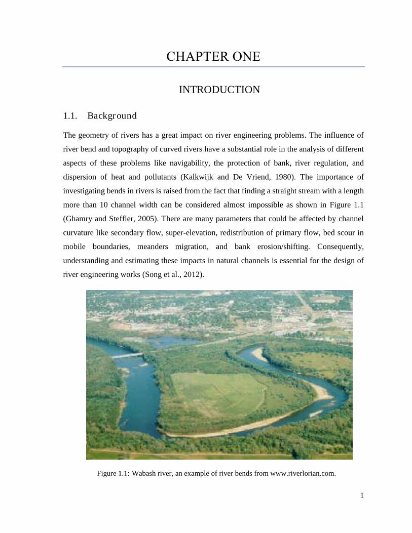
The geometry of rivers has a great impact on river engineering problems. The influence of
river bend and topography of curved rivers have a substantial role in the analysis of different
aspects of these problems like navigability, the protection of bank, river regulation, and
dispersion of heat and pollutants (Kalkwijk and De Vriend, 1980). The importance of
investigating bends in rivers is raised from the fact that finding a straight stream with a length
more than 10 channel width can be considered almost impossible as shown in Figure 1.1
(Ghamry and Steffler, 2005). There are many parameters that could be affected by channel
curvature like secondary flow, super-elevation, redistribution of primary flow, bed scour in
mobile boundaries, meanders migration, and bank erosion/shifting. Consequently,
understanding and estimating these impacts in natural channels is essential for the design of
river engineering works (Song et al., 2012).
Figure 1.1: Wabash river, an example of river bends from www.riverlorian.com.
2
The flow pattern in such channels is considered fairly complex because fluid particles follow
helical paths instead of moving parallel to the axis of the channel. Thus, it could be considered
that the helical flow is a combination of two flows, the main flow which is approximately
parallel to the channel axis and the secondary circulation (Kalkwijk and DeVriend, 1980). The
importance of studying the secondary or transverse flow comes from its partial influence on
the large-scale bed topography of natural alluvial channel bends. The primary flow is affected
by the transverse flow as well. In addition, it will be a good source for navigation and diffusion
studies in natural channels (Blanckaert and De Vriend, 2004). In channel bends, secondary
currents develop by skewing of cross-stream vorticity into a long stream direction. The skew
that results due to the secondary circulation carries the surface water quickly in the outer bank
direction and the bed water slowly towards the inner bank (Thorne et al., 1985). Rozovskii
(1961) and De Vriend (1980) measurements have proved that the secondary flow moves
toward the external bank near the upper part of the river and towards the internal bank in the
lower part of the river. As a result, the shear force which is in the same direction of the local
flow near to the lower part of the river (the bottom) turns slightly from the direction of the
mean flow (Duan, 2004).
The importance of the secondary flow or transverse flow lies in the followings (Falcon 1984):
It partially has the responsibility about the bed topography large-scale in natural
alluvial channel curves,
The possibility of dynamically interacting with the primary flow, and
It is beneficial for diffusion and navigation studies in natural waterways.
1.2. Shallow River Bends
This study deals with three-dimensional simulation of rivers with the following
characteristics:
Small depth comparing with width,
Small width comparing with the radius of curvature,
The scale of the horizontal length for the bottom variation is of the same order of the
width magnitude,
The friction of the flow is controlled,
3
The velocity longitudinal component controls the other ones, and
Small Froude Number.
1.3. The Mechanism of Secondary Flow
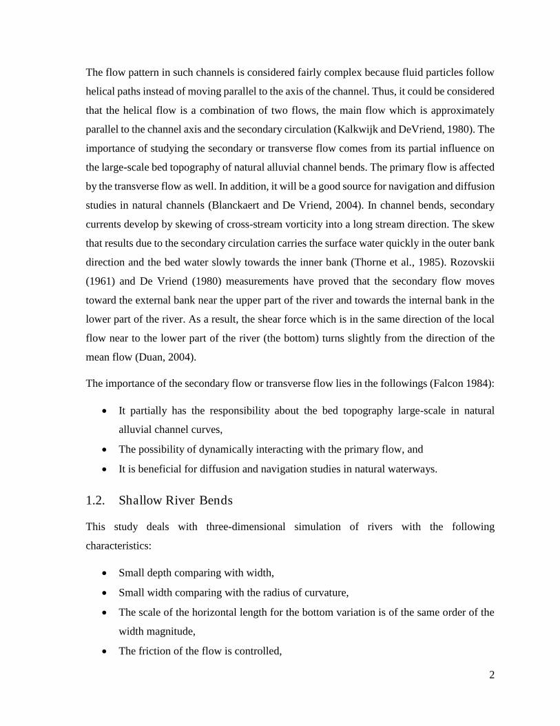
For the purpose of the present research, u is the component of secondary-flow velocity which
happens in planes perpendicular to the main direction of the motion (i.e. to the channel axis),
while v is the stream-wise velocity component and r is the radius of curvature. Thus, the
centrifugal acceleration because of the channel bend (the system of the coordinate shown is
cylindrical) is (v2/r). As shown in Figure 1.2, v varies from zero at the channel bed to a
maximum value at or close the surface of water. As a result, the centrifugal force s reaches its
maximum value near the surface of water and then decreases toward the bed (Falcon, 1984).
Figure 1.2: Illustrative sketch for curved channel flow (Falcon, 1984).
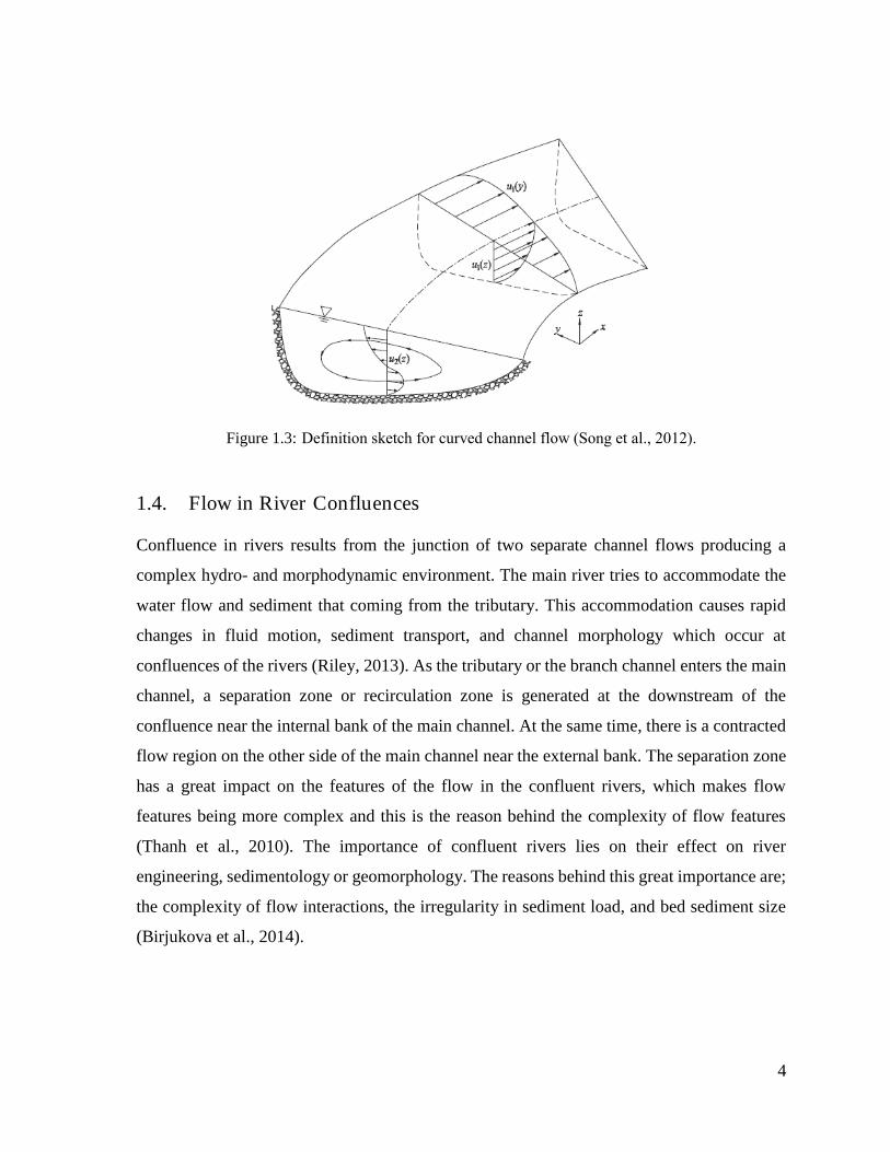
Several studies have shown that the secondary rotation in the plane normal to the direction of
the mean flow is produced by the sheared and curved flows. The local imbalance between the
centrifugal force that vary vertically and the cross-stream pressure gradient results in
generating the secondary flow and producing the typical motion of helical flow (Figure 1.3).
As a result of this imbalance situation, two flows exist; flow towards the inner bank of the
curve in the lower part of the water column and an outer flow near the surface of water (Song
et al., 2012).
4
Figure 1.3: Definition sketch for curved channel flow (Song et al., 2012).
1.4. Flow in River Confluences
Confluence in rivers results from the junction of two separate channel flows producing a
complex hydro- and morphodynamic environment. The main river tries to accommodate the
water flow and sediment that coming from the tributary. This accommodation causes rapid
changes in fluid motion, sediment transport, and channel morphology which occur at
confluences of the rivers (Riley, 2013). As the tributary or the branch channel enters the main
channel, a separation zone or recirculation zone is generated at the downstream of the
confluence near the internal bank of the main channel. At the same time, there is a contracted
flow region on the other side of the main channel near the external bank. The separation zone
has a great impact on the features of the flow in the confluent rivers, which makes flow
features being more complex and this is the reason behind the complexity of flow features
(Thanh et al., 2010). The importance of confluent rivers lies on their effect on river
engineering, sedimentology or geomorphology. The reasons behind this great importance are;
the complexity of flow interactions, the irregularity in sediment load, and bed sediment size
(Birjukova et al., 2014).
5
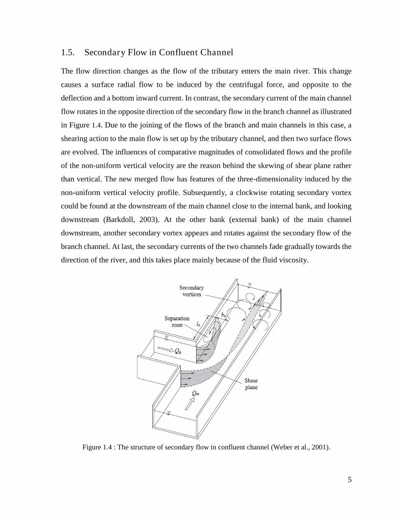
1.5. Secondary Flow in Confluent Channel
The flow direction changes as the flow of the tributary enters the main river. This change
causes a surface radial flow to be induced by the centrifugal force, and opposite to the
deflection and a bottom inward current. In contrast, the secondary current of the main channel
flow rotates in the opposite direction of the secondary flow in the branch channel as illustrated
in Figure 1.4. Due to the joining of the flows of the branch and main channels in this case, a
shearing action to the main flow is set up by the tributary channel, and then two surface flows
are evolved. The influences of comparative magnitudes of consolidated flows and the profile
of the non-uniform vertical velocity are the reason behind the skewing of shear plane rather
than vertical. The new merged flow has features of the three-dimensionality induced by the
non-uniform vertical velocity profile. Subsequently, a clockwise rotating secondary vortex
could be found at the downstream of the main channel close to the internal bank, and looking
downstream (Barkdoll, 2003). At the other bank (external bank) of the main channel
downstream, another secondary vortex appears and rotates against the secondary flow of the
branch channel. At last, the secondary currents of the two channels fade gradually towards the
direction of the river, and this takes place mainly because of the fluid viscosity.
Figure 1.4 : The structure of secondary flow in confluent channel (Weber et al., 2001).
6
1.6. Research Objectives
Due to the necessity to get satisfying predictions in river curves, 3D numerical models might
be considered useful for this purpose. These models depend on the three-dimensional flow
features consolidated with the complex spiral flow motion in the river curve. Nevertheless,
the large amount of computational time and possible numerical instability are important
matters that most of the 3D models suffer from (Song et al., 2012). In this study, the effects
of the secondary currents will be examined on the hydraulic structures and water surface
elevation in curved channels and confluences by employing a 3D OpenFOAM numerical
model (which will be explained later).
Thus, the present research aims at achieving the following objectives:
Assess the numerical model performance in the simulation of highly curved channels
and confluences.
Choose the suitable numerical model to simulate the behaviour of the flow in the river
bends and confluences.
Achieve the required components of the model by analysing the governing equations
in the mathematical model.
Examine and compare a number of turbulence models within the numerical model and
find the most accurate ones and optimal parameters.
Solve the model equations after finding out the best steady numerical schemes.
Compare the numerical results with comprehensive experimental and numerical data
that have been obtained by other researchers, taking into account the focus on velocity
and water depth.
1.7. Research Novelty
A number of studies including experimental or mathematical ones have been conducted to
examine the flow characteristics in curved open channels, river meanders or confluences.
However, understanding the dynamics of meanders is still incomplete, in particular with
respect to how the variation in channel characteristics controls the flow dynamics.
The research will implement the 3D OpenFOAM numerical model to simulate the horizontal
7
distribution of flow in curved rivers. In addition, the progress in unravelling and understanding
the bend dynamics will be considered. Furthermore, in this research several turbulence models
have been studied and evaluated to determine the best numerical models that could predict the
secondary current properties in the river bends and confluences with higher level of accuracy.
1.8. Structure of the Thesis
This research includes five chapters as detailed in below:
Chapter 1 presents the Introduction.
Chapter 2 deals with the literature review. This chapter focuses on the concept of the
secondary flows in river bends and confluences and the main factors that affect the secondary
flow through reviewing the previous studies that have been conducted in this field. Also, this
chapter takes into account the experimental and numerical studies on this topic. Furthermore,
the chapter is devoted to review different turbulence models that have been developed to
simulate secondary flows such as (i) Standard k-ε; (ii) Realizable k-ε; (iii) Launder-Reece-
Rodi RSTM (iv) k -equation large eddy simulation approach.
Chapter 3 presents the mathematical and numerical model. This chapter focuses on the
mathematical and numerical modelling and the theoretical concepts for these studies. The
chapter is devoted to improve the model by using OpenFOAM toolbox and illustrates the
methodology used to achieve this goal.
Chapter 4 deals with results and discussions. The summary of the main results is illustrated in
this chapter and a discussion for the main outcomes of the research is provided.
Chapter 5 presents the conclusion and suggestions for future research. This chapter includes
the conclusions of the research and proposes recommendations for subsequent studies.
8
CHAPTER TWO
2. LITERATURE REVIEW
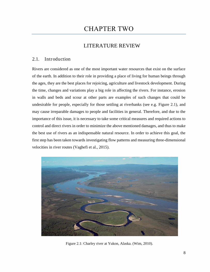
2.1. Introduction
Rivers are considered as one of the most important water resources that exist on the surface
of the earth. In addition to their role in providing a place of living for human beings through
the ages, they are the best places for rejoicing, agriculture and livestock development. During
the time, changes and variations play a big role in affecting the rivers. For instance, erosion
in walls and beds and scour at other parts are examples of such changes that could be
undesirable for people, especially for those settling at riverbanks (see e.g. Figure 2.1), and
may cause irreparable damages to people and facilities in general. Therefore, and due to the
importance of this issue, it is necessary to take some critical measures and required actions to
control and direct rivers in order to minimize the above mentioned damages, and thus to make
the best use of rivers as an indispensable natural resource. In order to achieve this goal, the
first step has been taken towards investigating flow patterns and measuring three-dimensional
velocities in river routes (Vaghefi et al., 2015).
Figure 2.1: Charley river at Yukon, Alaska. (Wim, 2010).
9
2.2. River Bends
Meandering is considered one of the common cases in most rivers. Rivers tend to change their
morphology in order to keep equilibrium with the ever-changing conditions imposed on the
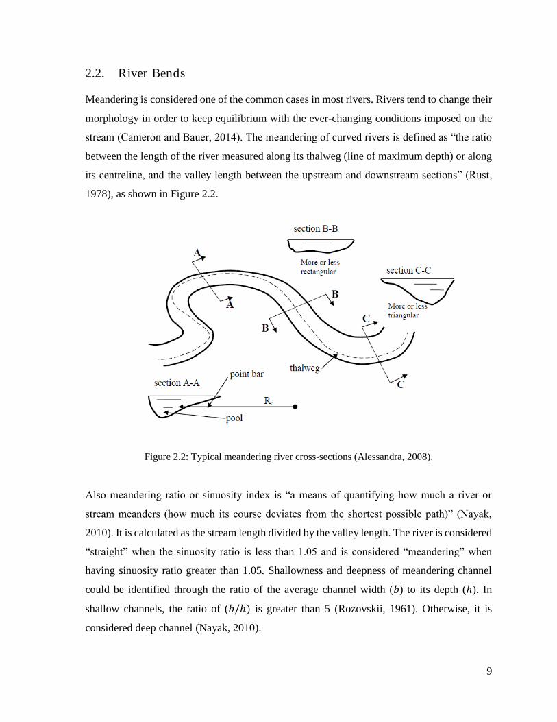
stream (Cameron and Bauer, 2014). The meandering of curved rivers is defined as “the ratio
between the length of the river measured along its thalweg (line of maximum depth) or along
its centreline, and the valley length between the upstream and downstream sections” (Rust,
1978), as shown in Figure 2.2.
Figure 2.2: Typical meandering river cross-sections (Alessandra, 2008).
Also meandering ratio or sinuosity index is “a means of quantifying how much a river or
stream meanders (how much its course deviates from the shortest possible path)” (Nayak,
2010). It is calculated as the stream length divided by the valley length. The river is considered
“straight” when the sinuosity ratio is less than 1.05 and is considered “meandering” when
having sinuosity ratio greater than 1.05. Shallowness and deepness of meandering channel
could be identified through the ratio of the average channel width (𝑏) to its depth (ℎ). In
shallow channels, the ratio of (𝑏/ℎ) is greater than 5 (Rozovskii, 1961). Otherwise, it is
considered deep channel (Nayak, 2010).
10
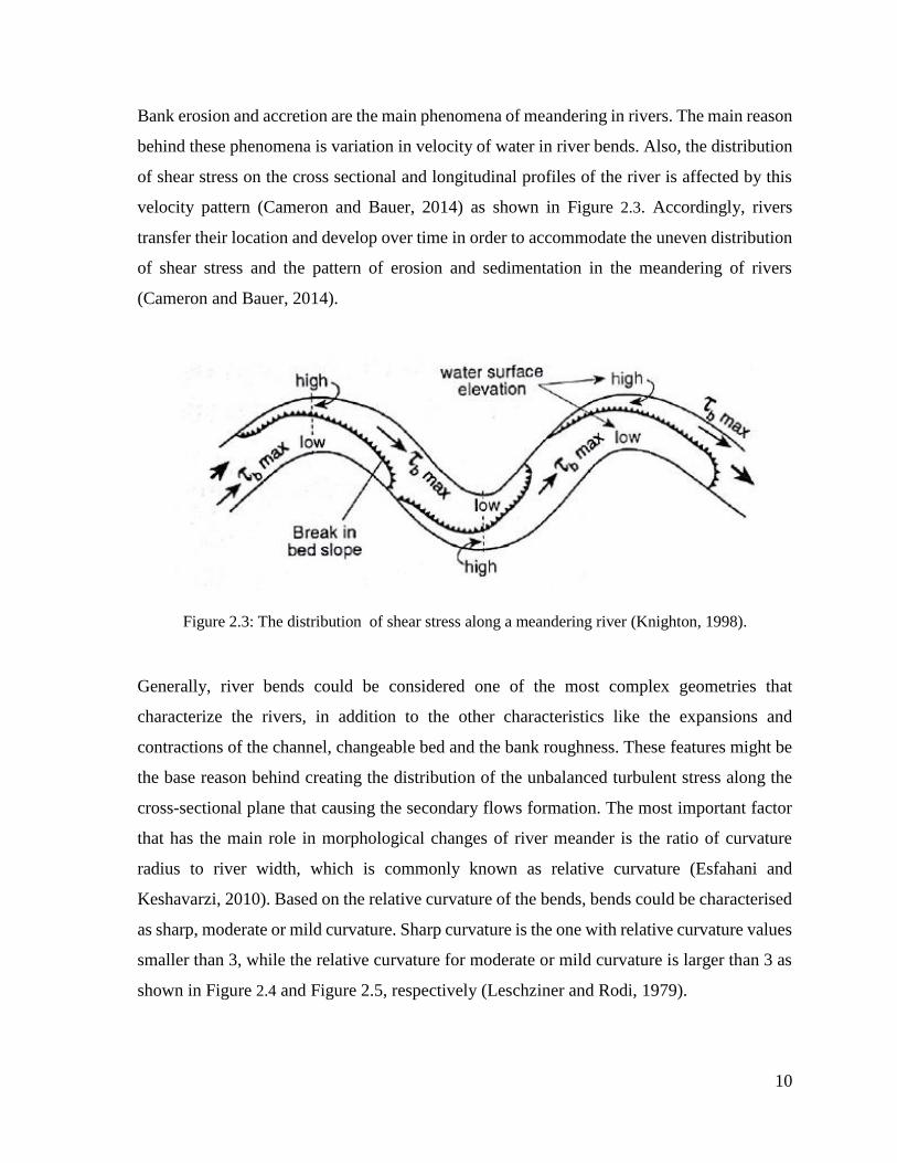
Bank erosion and accretion are the main phenomena of meandering in rivers. The main reason
behind these phenomena is variation in velocity of water in river bends. Also, the distribution
of shear stress on the cross sectional and longitudinal profiles of the river is affected by this
velocity pattern (Cameron and Bauer, 2014) as shown in Figure 2.3. Accordingly, rivers
transfer their location and develop over time in order to accommodate the uneven distribution
of shear stress and the pattern of erosion and sedimentation in the meandering of rivers
(Cameron and Bauer, 2014).
Figure 2.3: The distribution of shear stress along a meandering river (Knighton, 1998).
Generally, river bends could be considered one of the most complex geometries that
characterize the rivers, in addition to the other characteristics like the expansions and
contractions of the channel, changeable bed and the bank roughness. These features might be
the base reason behind creating the distribution of the unbalanced turbulent stress along the
cross-sectional plane that causing the secondary flows formation. The most important factor
that has the main role in morphological changes of river meander is the ratio of curvature
radius to river width, which is commonly known as relative curvature (Esfahani and
Keshavarzi, 2010). Based on the relative curvature of the bends, bends could be characterised
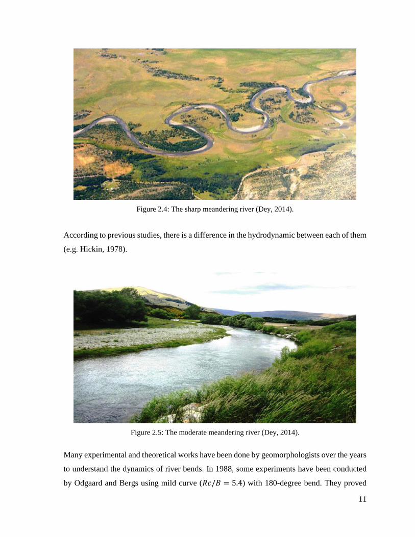
as sharp, moderate or mild curvature. Sharp curvature is the one with relative curvature values
smaller than 3, while the relative curvature for moderate or mild curvature is larger than 3 as
shown in Figure 2.4 and Figure 2.5, respectively (Leschziner and Rodi, 1979).
11
Figure 2.4: The sharp meandering river (Dey, 2014).
According to previous studies, there is a difference in the hydrodynamic between each of them
(e.g. Hickin, 1978).
Figure 2.5: The moderate meandering river (Dey, 2014).
Many experimental and theoretical works have been done by geomorphologists over the years
to understand the dynamics of river bends. In 1988, some experiments have been conducted
by Odgaard and Bergs using mild curve (𝑅𝑐/𝐵 = 5.4) with 180-degree bend. They proved
12
that changing in the curvature of the river bend affects the components of the velocity, bed
topography and the structure of the flow (Odgaard and Bergs, 1988). In 1990, Ikeda et al.
developed a three-dimensional mathematical model to simulate fully developed flow in mildly
curved open channels (Ikeda et al., 1990). A laboratory experiments were performed by Jung
and Yoon in 2000. They conducted the experiments in a mild 180-degree curved bend using
different bed materials. They concluded that extreme streamwise velocity in the upper part of
the curve is skewed inwards, and the bed materials effect does not change it (Esfahani and
Keshavarzi, 2010). The downstream velocity vertical profiles and secondary current were
presented through a model developed by Blankaert in 2001. The model is affected by several
factors such as Froude number, curvature ratio, normalized transversal velocity gradient, and
Chezzy coefficient. Consequently, good agreement was reached between the model and
experimental data of a strongly curved flow (Blanckaert, 2001). Also in 2001, some
experiments have been conducted in a sharp curved open channel by Blankaert and Graf.
They concluded that Rozovskii model overpredicts the strength of secondary circulation and
velocity distribution for this kind of bend (Blanckaert and Graf, 2001).
In 2003, Giri et al. used three sequential bends in a mild meandering flume for the
experiments. The bends were with and without the training structures of river in order to
examinethe impact of these structures on the pattern of the flow. For the case without river
training structures, they found that water flow is approximately uniform along the center of
the river and there is a graduate acceleration or deceleration near the two banks. In the other
case of bends with river training structures, they found that in the external bank of second
bend, there is dead area generated all over the bank. This situation might occur because of
existence of training structures inside the previous bend (Giri et al., 2003).
Turbulent structures in strongly open channel bends have been investigated by Blankaert and
De Vriend in 2004 and 2005 (Blankaert and De Vriend, 2004; Blankaert and De Vriend,
2005). Three physical models of multi-bend meandering rivers were designed by Esfahani in
2009, and Esfahani and Keshavarzi in 2009 as well, to examine the structure of the flow inside
the inner part of mild and strongly curved bend and outside meandering rivers (Esfahani,
2009; Esfahani and Keshavarzi, 2009). Also in 2009, a new equation for super elevation in
sharp curved open channels is presented by Akhtari et al. (2009).
13
Consequently, in order to predict the distribution of bed shear stress in the bends of rivers and
open channels, it is essential to study the influence of secondary flow and the distribution of
velocity on flow pattern. Therefore, a lot of studies have been carried out on the structures of
secondary flow and the distribution of shear stress at bend routes.
2.3. Secondary Flow in River Bends
The characteristics of flow could be considered more complicated in channel bends than those
in straight ones (Lien et al., 1999). The particles of the fluid follow a spiral path instead of
moving more or less parallel to the axis of the channel (Kalkwijk and De Vriend, 1980). In
addition to the turbulence and the 3D nature of flow, several factors could be the reason behind
this complexity such as bed topography and depth variations, which are generally under the
influence of erosion, sediment transport, and sedimentation processes. In river bends, the
centrifugal force affects the flow once it enters the bend. Based on the radius of the bend and
the depth direction due to the velocity variation, this force could be different. As a result to
the centrifugal force in river bends, the lateral gradient on water surface leads to the lateral
pressure gradient at cross section. One of the most dominant features of the flow in curved
open channels is secondary currents (Blanckaert and De Vriend, 2004). Secondary currents
are defined as "currents that occur in a plane normal to the axis of primary flow" (Thorne et
al., 1985). The imbalance between the gradient force of the transverse water surface and
centrifugal force over the depth occurs due to the vertical variation of the primary flow
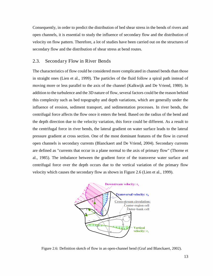
velocity which causes the secondary flow as shown in Figure 2.6 (Lien et al., 1999).
Figure 2.6: Definition sketch of flow in an open-channel bend (Graf and Blanckaert, 2002).
14
The secondary flow moves in a helical path towards the outer wall near the water surface and
towards the inner wall near the bed. Normally in a straight river, the core of high velocity flow
is located near the centre of the river. In the river bend and as the flow enters the bend, a
decreasing in the water depth near the inner bank occurs due to the transverse inclination of
the free water surface. Decreasing the flow depth in the inner bank of the river is associated
with the increasing of the flow velocity at the same side. However, near the downstream of
the river, the velocity structure will change because of the centrifugal force and the exchange
of momentum between horizontal layers due to transverse circulation which result in
transferring the higher velocity near the outer bank. Probably, the high velocity stays adjacent
to the outer bank for a long distance in the downstream direction unless meanders occur again
in the river causing another change in the velocity structure. Until now, extensive researches
have been undertaken for better understanding of the flow in river curves and the scour pattern
in meanders (Vaghefi et al., 2015).
2.4. Experimental and Numerical Studies
The existence of spiral flow pattern in channel bends was reported first by Thomson in 1876.
The reason behind this spiral flow is the interactions between the secondary current and
absence of regulation in velocity profile along the channel (Thomson, 1876). In 1943, an
experiments include two 180-degree bends have been carried out by Mockmore. He measured
longitudinal velocity profiles, and finally he reported that the flow close to the interior wall is
more than that near the exterior wall. Furthermore, he found the flow pattern in the channel
bends. He also proved that the distribution of velocity in the cross section would be in a way
that the multiplication of tangential velocity and radius of curvature would result in a constant
value (Mockmore, 1944). Flow in river bends has been studied by Shukry in 1949. He
introduced a criterion for the secondary flow strength. The criterion includes the kinetic
energy ratio of lateral flow to that of the main flow. Also, he concluded that in the curve of
the river, the kinetic energy of the longitudinal orientation is larger than that of the lateral flow
(Shukry, 1950). The relation that determined the specific length for when the secondary flow
has the maximum strength was offered by Rozovskii in 1961. Accordingly, he concluded that
for developing secondary flow, it should be a bend with a central angle of at least 100-degrees
for shallow channels, and a central angle of 180-degrees for deep ones. Also he observed that
15
the favourable results for velocity profile could be obtained from the logarithmic distribution
probability (Rozovskii, 1961). Shear stress and velocity distribution have been studied by
Ippen and Drinker in 1962. A trapezoidal meandering bend with varying entrance conditions
has been used in that study. They injected dye into the water and traced their paths. Thereafter,
they observed that the dye chain would direct towards the inner bank in the bed of the channel,
and towards the outer bank near the water surface. This phenomenon has been referred to as
the effect of wall friction on flow field. Moreover, the relationship between radius of curvature
and maximum shear stress has been determined as well (Ippen and Drinker, 1962).
The numerical simulation for turbulent flow in 180-degree sharp curve has been used by
Leschziner and Rodi in 1979 using k-ε model. They supposed absence of hydraulic jump and
flow separation. They observed that the higher velocity tends to be closer to the outer bank of
the channel near the end of the bend (Leschziner and Rodi, 1979). Also in 1979, the effect of
secondary flow on the distribution of bed shear stress was investigated by Nouh and
Townsend. According to their results, the effect of the generated secondary flow remains after
the bend exit and continues towards the downstream bend (Nouh and Townsend, 1979).
A field investigation was conducted by De Vriend and Geldof in 1983. The study that has
been conducted in Dommel which is a river in Netherlands, included a numerical simulation
of flow within a short period of time. The section included two sequential curves. Both of
them were in 90-degree and in the same direction with a short straight connection between
them. The results revealed that at the beginning of the bend, the maximum velocity is found
near the inner bank of the river, while maximum velocity at the end of the bend tends to be
oriented to the outer bank of the river (De Vriend and Geldof, 1983). A mathematical model
was presented by Odgaard in 1986 to simulate bed changes in sinusoidal alluvial rivers.
According to this model, there is a big interaction from the secondary flow component and
the transverse bed slope towards the curvature changes. Therefore, a model was developed to
provide an accurate prediction of flow and bed features in meandering alluvial channels
(Odgaard, 1986). Bergs studied in 1990 the flow pattern and topographical changes in the bed
of the channel by conducting an experimental study on a U-shaped flume with trapezoidal
section and live bed. He concluded that the flow takes a spiral form when entering the bend
and then it expands within a distance of 3 to 5 meters from the bend. Soon after, it completely
16
disappears at the end of the bend (Bergs, 1990).
In 1998, a 3D hydrodynamic model was developed for flow in bends by Jian and
McCorquadale. This hydrodynamic model had the capability to model the changes for the free
surface and bed topography (Jian and McCorquadale, 1998). The flow pattern was
investigated by Lien et al. in 1999 through 90 and 180 degree-bends and using depth averaged
two-dimensional model. The influence of the secondary flow was determined in the model
using the calculation of distributed tensor of the stress. In addition to the spread stresses, a
comparison between the important forces that exist in the flume was conducted. The results
showed a difference between the secondary flows in 180-degree bend and 90-degree bend.
The former is stronger than the latter (Lien et al., 1999). In 180-degree mild bend, the flow
pattern and bed topography were studied by Jung and Yoon in 2000. Generally, they observed
that in mild curves and with any kind of bed material, the higher velocity directed towards the
interior bank at the first half of the entrance zone of the curve. However, while the higher
velocity moving towards the end of the bend, its location will transmit gradually towards the
exterior bank (Vaghefi et al., 2015). Also in 2000, a 3D flow pattern in open channels was
studied by Wu et al. They considered sediment as bed and suspended loads in a curve with
180-degree. Secondary flow was predicted well by this model. The twist angle of velocity
vector was specified as well, which was averaged. Their conclusion included that higher
velocity tends to be near the outer bank while lower ones direct towards the inner bank.
Consequently, the water depth is lesser near the inner bank than near the outer bank (Wu et
al., 2000).
In 2002, an experimental and numerical analysis in meandering rivers was conducted by
Shams et al. They concluded that there is resemblance in the results between the measured
mean parameters of the flow and the numerical model. However, the turbulence parameters
generated by the measurements are varying from those results (Shams et al., 2002). Using the
Large Eddy Simulation Method (LES), the flow pattern in a mildly curved river bend was
modelled by Booij in 2003. A comparison was made between the Reynolds stresses in the
channel and the results of LES. The stresses could be used for studying the longitudinal
momentum displacement. Also, it can be used to examine the impact of transporting the
secondary flow momentum on longitudinal momentum (Booij, 2003a). The velocity
17
distribution in flume bends was studied by Blanckaert and Graf in 2004 in addition to the
boundary shear stress, and features and form of bed topography in the bends. A semi 3D model
was used and a central zone was considered as a cell, which can twist to determine bed
topography in flume bends (Blanckaert and Graf, 2004).
Secondary flow, velocity distribution pattern, and boundary shear stress in open channels were
examined by Yang in 2005. In this study, velocity distribution and shear stress were applied
to laminar, steady, and turbulent flows. Also, the equations that govern the boundary shear
stress and Reynolds stress distribution were stated (Yang, 2005). An experimental study on a
local scour in 90-degree curved flume was carried out by Sui et al. in 2006. In this study, the
influence of some parameters such as Froude number, the width and the slope of the protective
wall, and the size of bed particle on the amount of scour near the bed was analysed (Sui et al.,
2006). Experimental and numerical studies for flow pattern in the curve of 90-degree were
done by Naji et al. in 2010. Their conclusion included that streamlines orient towards the inner
wall of the channel in the level close to bed, while the orient towards the outer wall of the
channel in the level close to the water surface (Naji Abhari et al., 2010). Also in 2010,
Barbhuiya and Talukdar conducted an experimental study for flow of 3D pattern and scour in
a bend of 90-degree. In this study, some elements were measured like velocity-time
components, turbulent tension, and Reynolds shear stress in different vertical sections using
Acoustic Doppler Velocimeter (ADV). According to the results, they indicated that the
maximum measured velocity was 1.61 times the mean velocity. The maximum scour hole
depth was found (Barbhuiya and Talukdar, 2010).
Two Computational Fluid Dynamics (CFD) codes (RANS and LES) were used by Stoesser et
al. in 2010 to compute flow in meandering channel. Different turbulence closure approaches
were employed to solve the Navier-Stokes equations. According to the comparison conducted
in this study between the results that obtained from the two codes and the experimental data
from the physical model, they indicated that the primary helical flow pattern in meander was
predicted by both of the LES and RANS simulations, in addition to the happening of an outer-
bank secondary cell (Stoesser et al., 2010). An experimental study for 3D flow pattern and
erosion was conducted by Uddin and Rahman in 2012 using Acoustic Doppler Current Profile
(ADCP) velocity meter in Jamuna river bend. The 3D velocity of the flow and shear stress
18
were measured in this study in the place close to the bed of the river. A model was presented
to predict the erosion on the bend based on the flow processes. Finally, a comparison between
the model and the real data recorded from the observations of the mentioned river was done
(Uddin and Rahman, 2012). In 2014, a numerical study was carried out by Liaghat et al. for
the hydraulic of flow in a U-shaped channel with changing width using SSIIM software. The
study addressed the 3D flow velocity components, shear stress, and the strength of secondary
and spiral flow (Liaghat et al., 2014). Also in 2014, Depth-Averaged Method (DAM) was
used by Vaghefi et al. in 180-degree sharp bend to study and analyse the distribution of shear
stress near the channel’s bed. The results indicated that the maximum shear stress occurs at
the beginning of the bend in the 40-degree cross section close to the interior wall of the channel
(Vaghefi et al., 2014).
2.5. The Strength of Secondary Flow
Many factors could influence the strength of secondary flow, the distribution of velocity, and
bed shear stress distribution in river bends such as: radius/channel width ratio (𝑅/𝐵), channel
width/flow depth ratio (𝐵/𝐻), and (𝐻/𝑅), which equal to[(𝐻/𝐵) × (𝐵/𝑅)]. According to
that, many studies were performed to examine these factors and determine the most influential
one. The main parameter according to (Rozovskii, 1961; Engelund, 1974) that affects the
circulation level which associated with the secondary flow in the bend is 𝐻/𝑅.The decrease
of 𝑅/𝐵 causes an increase in the circulation induced by the secondary flow, which comply
with the results reported by Hickin based on field studies in 1978 (Hickin, 1978). According
to Hickin and Nanson (1984), a decrease of 𝑅/𝐵 causes an increasein the rate of bend
migration. However, at 𝑅/𝐵 ≈ 2, a decrease in the bend migration rate starts after this point
(Hickin and Nanson, 1984). The influences of 𝑅/𝐵 and 𝐶𝑓−1𝐻/𝐵 (where 𝐶𝑓 is the bed friction
coefficient) on bend flow was studied by Blanckaert (2011) and Ottevanger et al. (2011). They
used nonlinear one-dimensional (1D) analytical models in their study. Consequently, the
performance of the models that used were comparatively good for both of the moderate and
sharp bends (Blanckaert, 2011; Ottevanger et al., 2011). The flow in river bends and curved
channels were studied using different types of numerical models. The main purpose of these
models was to clarify the details of flow in bends and meandering channels (Zeng et al., 2008).
19
2.6. Hydrodynamic Modelling of Bend Flow
Basically, there are two categories of hydrodynamic models for flow in river bends: linear
models, and nonlinear models. These models are mainly used to combine the impact of the
secondary current in bends. Linear and nonlinear aspects of flow development and bed
perturbations in evolving bends were studied by Seminara and Tubino in 1989. In this study,
a methodical therapy for such cases was provided (Seminara and Tubino, 1989). A general
mathematical framework was established by Camporeale et al. in 2007 to compare and
provide hierarchy of meandering models. A description for the interrelationships among the
physical processes, which occur in curved rivers, were also explained in this mathematical
framework (Camporeale et al., 2007). In spite of the considerable advancement in unraveling
and understanding the dynamics of meander that was let out by linear models, the negligence
of high-curvature effects was one of the reasons that made them defective (Blanckaert and De
Vriend, 2010; Seminara, 2006) in addition to the limited validity to weak curvatures (Yeh and
Kennedy, 1993; Blanckaert and De Vriend, 2003). Due to the fundamental drawback of the
linear approach, a number of nonlinear models (Jin and Steffler, 1993; Yeh and Kennedy,
1993) were suggested although they are difficult to code and more expensive to compute.
Blanckaert and De Vriend worked to improve the accuracy of the linear models. Their
development to rectify the model was by inclusion of a correction factor to the linear
prediction model for tight bends. The feedback between the velocity of the downstream and
the secondary circulation is incorporated by this correction factor (Blanckaert and De Vriend,
2003). According to Johannesson and Parker (1989) and Blanckaert and Graf (2004), for a
strong bend curvature where the maximum velocity occurs in the lower part of the water
column, a boundary shear stress and the redistribution of downstream velocity will be
presented. The dominant mechanism for this redistribution is the interaction between the
secondary circulation and the advective transport of downstream momentum. Subsequently,
they developed a nonlinear model through incorporating these terms into the formulation of
linear model. Furthermore, due to the continuous variation of the radii of curvature in the
streamwise direction of meandering bends, the accelerations of convective flow occur and
cross-circulation changes from section to section (Termini and Piraino, 2011). The cross
sectional flow according to their model was decomposed into two parts: the first part is the
20
cross-circulation, caused by channel curvature, and the second part is the convective
component, which is established due to the variation of the channel curvature. Thus, the
distribution of the radial velocity component is determined based on the summation of the
convective and cross-circulation distribution components. However, the vertical average of
the cross-circulation in the model provided by Dietrich and Smith (1983) and Yalin (1992)
was a zero and a net of flux of mass is formed in the radial direction.
2.7. Modelling the Effects of Secondary Flows
The development of the secondary flow in the channel bends can be attributed to the local
imbalance between the centrifugal forces and the transverse pressure forces, which is
generated by the super-elevation of the water surface. The influence of secondary currents on
bend flow can be predicted using mathematical and numerical models (Song et al., 2012). The
effective stresses should be included in the depth-averaged calculations as Flokstra showed if
the secondary flows were to be predicted (Flokstra, 1977). An equation was developed by
Johannesson and Parker to predict the lateral distribution of the depth-averaged main flow
velocity in curved rivers (Johannesson and Parker, 1989). They reported that the reason behind
the considerable external redistribution of main flow velocity is the convective transfer of
main flow momentum by the secondary flow. Also, they quantified the redistribution of
primary momentum phenomenon due to the secondary flow in the case of uniform flow bends.
A hybrid integral-differential formulation was derived by Yeh and Kennedy (1993) in constant
radius open channels. And in order to formulate the secondary flow and the influences of
curvature on the profile of the primary-flow velocity, they used the integrated equations for
the flux of the moment of momentum (Yeh and Kennedy, 1993). They clarified the necessity
of the consideration of moment formulation for elucidating the interaction between the
secondary and main flows. The most popular methods that have been widely used for
describing the bend flow in the problems of shallow water are:
2D Vertically Averaged and Moment (VAM) model
This method is based on combining the depth-averaged continuity and momentum equations
with additional moment-of momentum equations. The latter is derived from the balance
21
among the momentum fluxes in terms of the convective, pressure gradient, and stress as
follows (Ghamry and Steffler, 2005):
𝜕ℎ
𝑑𝑡+
𝜕𝑞𝑗
𝜕𝑥𝑗= 0 (2. 1)
𝜕𝑞𝑗
𝑑𝑡+
𝜕
𝜕𝑥𝑗(𝑞𝑖𝑞𝑗
ℎ) + 𝑔ℎ
𝜕
𝜕𝑥𝑗
(ℎ + 𝐻) −1
𝜌
𝜕𝜏𝑖𝑗
𝜕𝑥𝑗+
1
𝜌𝜏𝑏𝑗 −
1
3
𝜕
𝜕𝑥𝑗(ℎ��𝑖��𝑗) = 0 (2. 2)
𝜕��𝑖
𝑑𝑡+
𝜕
𝜕𝑥𝑗(𝑞𝑗��𝑖
ℎ) + ��𝑘
𝜕
𝜕𝑥𝑘(𝑞𝑖
ℎ) =
2
3[4𝜏𝑖𝑗
ℎ𝜌
𝜕𝑧𝑚
𝜕𝑥𝑗−
4𝜏𝑖𝑧
ℎ𝜌+
2
ℎ𝜌𝜏𝑏𝑖] (2. 3)
where;
𝑖= 1, 2, 𝑡= time; 𝑞1, 𝑞2= flow discharge per unit width in the x-, y- directions, respectively;
𝑔= acceleration of gravity; ℎ= flow depth; 𝐻= bottom elevation; 𝜏𝑖𝑗= vertically averaged total
turbulent shear stress in the ij-direction; 𝜏𝑏𝑖= bed shear stress; ��1, ��2= velocities at the water
surface in excess of mean velocity in the x-, y-directions, respectively; and 𝑧𝑚= mean flow
depth.
Two shortcomings can be indicated when using this method. Firstly, more computational
efforts are required because the solution needs additional transport equations. Secondly, the
friction factor impacts, curvature ratio, and the distribution of the transversal velocity are not
discernible in the mathematical formulation (Blanckaert and De Vriend, 2003).
The Depth-Stress Averaging Approach
The Depth-Stress Averaging Approach adopts the average time in the 3D Navier–Stokes
equations. Using the average depth in the equations result in vertically averaged and 3D
Reynolds equations as shown in Equation (2. 4) (Ahmadi et al., 2009):
𝜕
𝑑𝑡∫ 𝑢𝑖(𝑧)𝑑𝑧 +
𝜕
𝜕𝑥𝑗∫ 𝑢𝑖(𝑧)𝑢𝑗(𝑧)𝑑𝑧 + 𝑔ℎ
𝜕(𝐻 + ℎ)
𝜕𝑥𝑖
𝐻+ℎ
𝐻
𝐻+ℎ
𝐻
− ∫ 𝑣𝜕2𝑢𝑖(𝑧)
𝜕𝑥𝑗𝜕𝑥𝑗𝑑𝑧 + 𝑔𝑛2
𝑈𝑖√𝑈𝑗𝑈𝑗
ℎ1 3⁄= 0
𝐻+ℎ
𝐻
(2. 4)
where;
22
𝑢𝑖(𝑧)= vertical distribution of i-component velocity; 𝑣= kinematic eddy viscosity; 𝑛=
Manning’s roughness coefficient; and 𝑈𝑖= the depth averaged velocity in i-direction.
The main advantage of this approach is that it is not necessary to solve additional transport
equations because the influence of the secondary flow can be activated with any vertical
velocity profile given. As a result, difference between the vertically varying velocity and the
velocity of the mean flow is integrable. In order to include the characteristics of the channel
and flow variables, like the depth of the flow and the channel curvature, the equation in the
above needs calibration parameters.
2.8. The Secondary Currents Velocity Profiles
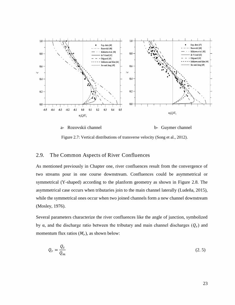
To illustrate the velocity profiles of secondary currents, Figure 2.7 shows a comparison
between the empirical and the theoretical profiles of transverse velocity and the experimental
results provided by Rozovskii (1961) and Guymer (1998). The following points can be
highlighted (Song et al., 2012):
The classical formula developed by De Vriend (1976) has a robust mathematical
background and been widely tested in the numerical simulation of bend flow. This formula
considers the no-slip boundary condition at the bottom region and, unlike other theoretical
profiles that overestimate the transverse velocity, it provides outputs with a good
approximation to the observed data over the depth.
The perpendicular component (due to the curvature of the main flow) and the parallel
component (due to the curvature of the main flow) to the main flow direction were
considered explicitly in the derivation procedure (De Vriend, 1976).
Although the research by Seo and Jung (2010) is in need for additional verifications under
various conditions, the provided performance curve appeared to be satisfactory (Seo and
Jung, 2010).
This study used the vertical distribution of transverse velocity proposed by De Vriend
(1976) to reflect the effect of secondary flow in the mathematical and numerical models.
23
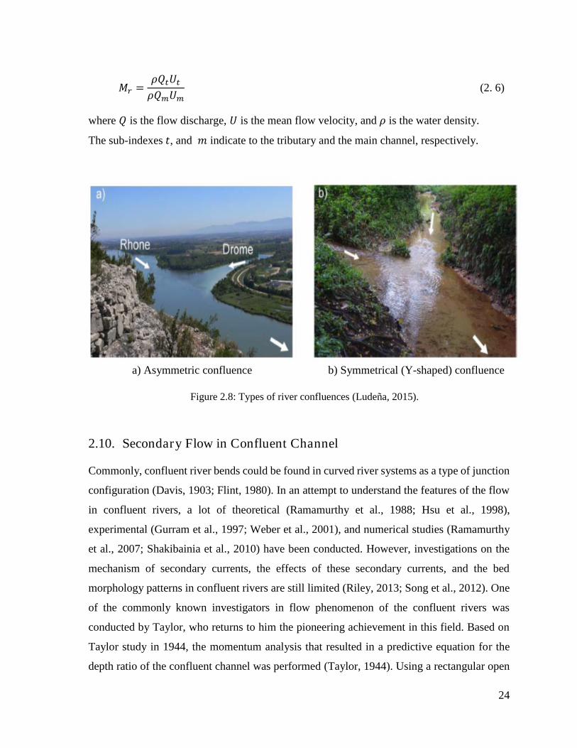
2.9. The Common Aspects of River Confluences
As mentioned previously in Chapter one, river confluences result from the convergence of
two streams pour in one course downstream. Confluences could be asymmetrical or
symmetrical (Y-shaped) according to the planform geometry as shown in Figure 2.8. The
asymmetrical case occurs when tributaries join to the main channel laterally (Ludeña, 2015),
while the symmetrical ones occur when two joined channels form a new channel downstream
(Mosley, 1976).
Several parameters characterize the river confluences like the angle of junction, symbolized
by α, and the discharge ratio between the tributary and main channel discharges (𝑄𝑟) and
momentum flux ratios (𝑀𝑟), as shown below:
𝑄𝑟 =𝑄𝑡
𝑄𝑚 (2. 5)
a- Rozovskii channel b- Guymer channel
Figure 2.7: Vertical distributions of transverse velocity (Song et al., 2012).
24
𝑀𝑟 =𝜌𝑄𝑡𝑈𝑡
𝜌𝑄𝑚𝑈𝑚 (2. 6)
where 𝑄 is the flow discharge, 𝑈 is the mean flow velocity, and 𝜌 is the water density.
The sub-indexes 𝑡, and 𝑚 indicate to the tributary and the main channel, respectively.
2.10. Secondary Flow in Confluent Channel
Commonly, confluent river bends could be found in curved river systems as a type of junction
configuration (Davis, 1903; Flint, 1980). In an attempt to understand the features of the flow
in confluent rivers, a lot of theoretical (Ramamurthy et al., 1988; Hsu et al., 1998),
experimental (Gurram et al., 1997; Weber et al., 2001), and numerical studies (Ramamurthy
et al., 2007; Shakibainia et al., 2010) have been conducted. However, investigations on the
mechanism of secondary currents, the effects of these secondary currents, and the bed
morphology patterns in confluent rivers are still limited (Riley, 2013; Song et al., 2012). One
of the commonly known investigators in flow phenomenon of the confluent rivers was
conducted by Taylor, who returns to him the pioneering achievement in this field. Based on
Taylor study in 1944, the momentum analysis that resulted in a predictive equation for the
depth ratio of the confluent channel was performed (Taylor, 1944). Using a rectangular open
a) Asymmetric confluence b) Symmetrical (Y-shaped) confluence
Figure 2.8: Types of river confluences (Ludeña, 2015).
25
channel, a laboratory experiment was carried out by Webber and Greated in 1966 to
characterize the bulk flow variables at the intersections of the channels (Webber and Greated,
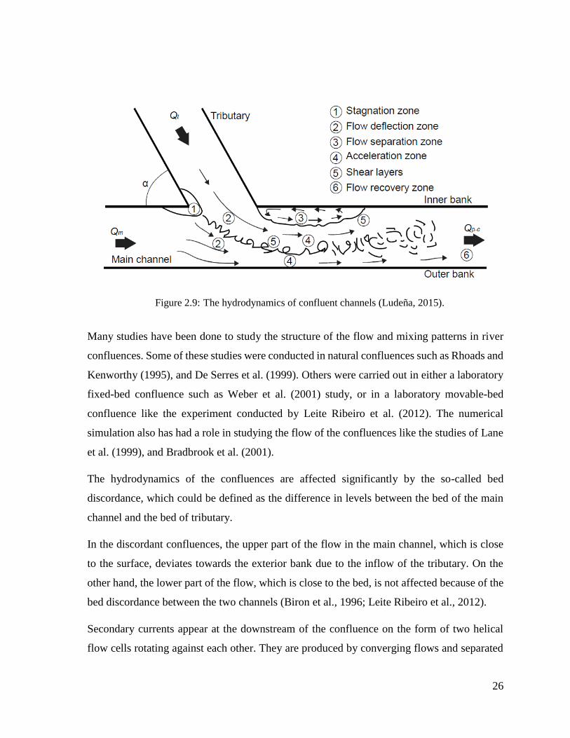
1966). The characteristics of six main regions in confluent rivers were specified and described
by Best in 1987 as described below (Figure 2.9) (Best, 1987):
Stagnation zone: It lies in the area of the confluence at the upstream corner. This zone
is followed by the deflection of the flow in the two connected channels, and it is
accompanied with a reduction in the flow velocity and shear stress, and an increase in
the pressure and flow depth.
Flow deflection zone: This zone is located immediately after the stagnation zone,
where the deflection of the flow of the main channel occurs towards its external bank
due to the incoming tributary flow.
Flow separation zone: This zone exists at the corner of downstream junction due to
the changing in direction of the flow of the tributary. The separation of the flow from
the internal bank of the main channel could be accompanied with this zone in addition
to the low pressures and flow recirculation.
Acceleration zone: This zone lies in the region confined between the separation zone
and the external bank of the main channel at the downstream of the junction. It is called
acceleration zone due to the high velocity of the flow, which could reach the maximum
at this area in addition to the increasing in the shear stress.
Shear layers: These layers could be found in two regions in the main channel due to
the high velocity gradients. The first one is located in the region confined between the
recirculation zone and the surrounding flow, while the second one is located in the
buffer zone between the two flows of the tributary and main channel.
Flow recovery zone: This zone occurs after the ending of the confluence
hydrodynamics impact on the flow. The two flows from the tributary and the main
channel come together towards the downstream of the main channel.
26
Many studies have been done to study the structure of the flow and mixing patterns in river
confluences. Some of these studies were conducted in natural confluences such as Rhoads and
Kenworthy (1995), and De Serres et al. (1999). Others were carried out in either a laboratory
fixed-bed confluence such as Weber et al. (2001) study, or in a laboratory movable-bed
confluence like the experiment conducted by Leite Ribeiro et al. (2012). The numerical
simulation also has had a role in studying the flow of the confluences like the studies of Lane
et al. (1999), and Bradbrook et al. (2001).
The hydrodynamics of the confluences are affected significantly by the so-called bed
discordance, which could be defined as the difference in levels between the bed of the main
channel and the bed of tributary.
In the discordant confluences, the upper part of the flow in the main channel, which is close
to the surface, deviates towards the exterior bank due to the inflow of the tributary. On the
other hand, the lower part of the flow, which is close to the bed, is not affected because of the
bed discordance between the two channels (Biron et al., 1996; Leite Ribeiro et al., 2012).
Secondary currents appear at the downstream of the confluence on the form of two helical
flow cells rotating against each other. They are produced by converging flows and separated
Figure 2.9: The hydrodynamics of confluent channels (Ludeña, 2015).
27
by a shear layer as reported by Mosley (1976). Many studies paid a great attention in studying
these secondary currents in river confluences. Some of them were carried out in the field such
as (Rhoads and Kenworthy, 1995, 1998; Rhoads, 1996; Rhoads and Sukhodolov, 2001; Riley
et al., 2015) and others in the laboratory such as (Mosley, 1976; Weber et al., 2001). Whereas
(Bradbrook et al., 1998) have conducted their investigation on the secondary currents by the
means of numerical models.
According to Rhoads and Kenworthy (1995), there is a similarity between the flow structures
of the river confluences and river bends because of the existence of the helical cells at the
downstream of the confluence, which are produced by the curvature in the flow deviation area.
The secondary currents in the asymmetrical confluences are more sophisticated (Rhoads and
Kenworthy, 1995; Rhoads and Sukhodolov, 2001) than those in the symmetrical confluences
(Rhoads and Sukhodolov, 2001) because the curvature adopted by the tributary inflow in the
asymmetrical confluences is greater than those in the symmetrical confluences, which leads
to more helical cells on the tributary side of the shear layer.
The momentum flux ratio affects the secondary currents. Noting that, these secondary currents
on the tributary side are larger than that on the main channel side (Rhoads and Kenworthy,
1995; Rhoads, 1996; Riley et al., 2015).
Bed discordance enhances the secondary flow, in addition to the planform curvature and
junction angle (Lane et al., 1999; Bradbrook et al., 2001; Riley et al., 2015). The secondary
currents are generated in absence of planform curvature for specific combinations of depth
and velocity ratio according to the numerical study of Bradbrook et al. (1998). The reason
behind the absence of secondary flow cells in a natural confluence in the Río Paraná
(Argentina) returns to the high form roughness and the high width to depth ratio as the
attribution of Parsons et al. (2007).
Two-dimensional approaches have been used in different studies to examine the numerical
simulation of river confluences, for either research purposes or for case studies (Ludeña,
2015). Due to the good agreement that have been obtained from the comparison between the
numerical results and field or experimental measurements, the simulation of the confluence
hydrodynamics by using three-dimensional models was recommended by Lane et al. (1999),
28
especially if the two-dimensional numerical model does not execute any alteration for the
influence of the secondary current on the flow structure.
At present, the simulation of confluence hydrodynamics by using three-dimensional models
could be considered more common (Bradbrook et al., 2001; Shakibainia et al., 2010). Using
the unsteady turbulence models for these simulations were recommended by Parsons (2003)
in order to fully capture the flow structures due to the presence of shear layers.
29
CHAPTER THREE
3. MATHEMATICAL AND NUMERICAL MODEL
3.1. Introduction
The experimental investigation and theoretical calculation are considered the major methods
to predict the fluid flow processes. Although the actual measurement and experimental
investigations is the best approach to get accurate information about physical processes, it
could be too expensive. The use of the scaled models and conditions is the other choice to
predict the results to a full scale. However, this choice is not totally error-free.
Physical processes could be represented by a mathematical model which will be consequently
the basis of the theoretical predictions. The mathematical models of fluid dynamic problems
mainly contain a set of partial differential equations. Using the classic mathematical
techniques to solve these equations and predict many cases of practical interest might end up
with a questionable accuracy. The use of sophisticated computers and implementing
numerical methods would enhance the level of accuracy besides other advantageous such as:
low cost, speed, complete and detailed information, capability in simulating both realistic and
ideal conditions. On the other hand, the disadvantages of using the numerical calculation
would be: difficulties in finding a suitable mathematical model, geometric complexities,
strong nonlinearity, longer and again being more expensive to solve.
Mathematical model is considered the beginning point to any numerical method, which is
consisting of boundary conditions and a group of partial differential equations. The behaviour
of any flow, as described by conservation laws, depends largely on the general governing
equations. Developing a solving method designed for that specific group of equations might
be the best approach to get a simplification in the mathematical model (Mangani, 2010).
Thereafter, a suitable Discretization Method, which is an approximation to the set of
differential equations by an algebraic equation system for the variables at a number of discrete
points in time and space, is necessary to be implemented. The most popular discretization
methods are: Finite Volume Method (FVM), Finite Difference Method (FDM), and Finite
30
Element Method (FEM). The calculation of the variables is done at discrete locations, which
are defined by the Numerical Grid. The numerical grid is a discrete representation of the flow
domain in space and time through the use of a finite number of subdomains such as elements,
control volumes, etc. After that, a Finite Approximation technique has to be selected
considering the choice of the discretization method and the numerical grid. It is worth to note
that the accuracy of the solution would be affected by the choice of the discretization method,
development, coding, debugging and the speed of the solution method. As soon as the
discretization techniques build this large system of non-linear algebraic equations, it should
be solved using a Solution Method. The successive linearization for the equations is used in
these methods and the iterative techniques are always used to solve the resulting linear
systems. Generally, there are two levels of iterations. First, the inner iteration is used to solve
the linear equation. Second, the outer iteration is used to solve the non-linearity and coupling
of the equations. Finally, it is necessary to determine a suitable Convergence Criterion. It is
essential to set stopping conditions for the inner and outer cycles to get an accurate solution
to an effective manner. In order to determine whether the method is suitable or not, there are
certain properties that should be available in the numerical methods. The most important
properties are:
1. Consistency: The discretization must be exact as the spacing between the grids tends
to zero. In other words, the difference between exact and discredited equation, must
approach zero as ∆𝑡 → 0 and ∆𝑥 → 0.
2. Stability: The errors of the numerical solution process should be decreasing over the
iteration procedure. The methods that do not diverge are stable methods.
3. Convergence: The discretized equation solution should tend to the exact solution as
the spacing of the grid approaches zero. Since it is a very difficult task to demonstrate
this property, it is usually accepted to test grid-independence for a solution.
4. Conservation: The solution must respect conservation of physical quantities on both
local and global scales. This property is important because it limits solution error. Even
if on fine grids, non-conservative schemes can also lead to correct solutions,
conservative ones are usually preferred.
5. Boundedness: The solution should lie within proper bounds. Boundedness is difficult
to guarantee and often unbounded schemes have stability and convergence problems
31
as well.
6. Realizability: The model should provide physically realistic solutions for the
phenomena.
7. Accuracy: It is the property of well approximating the exact solution. In other words,
it is limiting the modelling, discretization, and iteration errors.
3.2. Numerical Model
Basically, there are three principles that govern the fluid motion: conservation of mass,
energy, and momentum. The continuity, energy and momentum equations are the results of
these principles. It is not easy to follow the track of these essential principles when the
situations become more complex. The basic equations are replaced by empirical
approximations, and mathematical calculations with numerical models. The numerical models
could come in different forms such as one, two, or three dimensions, and steady or unsteady
flow conditions etc. The derivations of basic principles are the base of all the numerical
models, which are required to make some forms of numerical approximation to solve these
principles considering their limitations. The model should be used in a right manner according
to what it was designed for or corresponds to the approximations that it was based upon,
otherwise, gross errors might appear in the predictions of the model. Therefore, it is important
to promote a basic awareness of how numerical models operate and how to draw attention to
some of the more common limitations that are implicit to this operation (Toombes and
Chanson, 2011).
3.2.1. Types of Numerical Models
Computational Fluid Dynamics (CFD) is defined as “a branch of fluid mechanics that uses
numerical methods and algorithms to solve and analyze problems involving fluid flows”
(Toombes and Chanson, 2011). CFD uses a numerical model of a high order accuracy to solve
a complex flow situation such as multi-fluid, three-dimensional, and thermodynamic effects.
All numerical models in real situation are considered CFD models even for a simple solution
of a backwater equation.
In order to analyze the fluid motion, two methods can be generally considered. First, describe
the flow pattern at all points of the field of the flow. Second, use finite or control-volume
32
analysis to examine the finite region. In general, the control volume approach is adopted by
most of the numerical models due to conservation properties.
Due to the real flow complexity, solving the governing equations is considered impossible
without using some simplifying assumptions, even when using complex models and fast
computers. The classification of the hydraulic models could be done through the
simplifications employed by the model. Number of fluid properties and dynamic assumptions
are associated with each category even though there are always exceptions to the rule
(Toombes and Chanson, 2011).
3.3. Open-Channel Flow
The open channel flow describes the flow with an open surface or free surface that is in touch
with the atmosphere. It could be natural such as rivers, streams, floodplains, and estuaries or
artificial like canals, flumes, spillways, culverts, and weirs drainage ditches. There is no free
surface in closed channels since they are full with fluid. The pressure forces are driving the
fluid in this kind of channels, while the fluid is driven by gravity force in open channels. The
basic force balance is between gravity and friction.
The discharges and water depths can be predicted based on channel geometry. Typically, in
such kind of problems, the fluid is water, the channel has a large size, and the flow is turbulent.
The free surface is treated under constant pressure since it is commonly at atmospheric
pressure. The open channel includes two side walls with a bottom, and satisfies the no-slip
condition. Due to friction in open channel along the boundary, the velocity always varies
across the channel sections. It is a complex profile, the maximum velocity usually occurs in
the mid plane around 20% below the surface. The main reason behind that is the secondary
currents that circulating from the boundaries towards the center causing a resistance at the
air/water interface. However, the maximum velocity occurs near the surface in the wide and
shallow channels with a velocity profile approximately logarithmic from the bottom to the
surface (Herreras and Izarra, 2013).
3.4. Free Surface Flows Model
There are a lot of cases that could be described by the shallow water model such as flood in
33
rivers, tidal fluctuations, waves on shallow beaches, estuary and bay flows, etc. Basically, it
is derived from 3D incompressible Navier-Stokes equations, by depth averaging of the
continuum mass and momentum balances (Dabaghi et al., 2005).
3.4.1. The Free Surface Flows Numerical Simulation
Generally, the numerical methods in various cases assumed to be either incompressible, or
compressible. Both of the incompressible Navier-Stokes equations or Euler compressible
equations could be satisfied for the velocity and pressure over the entire domain. Methods that
mix between an incompressible liquid and a compressible gas also have been considered.
Navier-Stokes equations are appropriate for the incompressible liquid, while for the
compressible gas the Euler's equations are more suitable. Free surface flows can be solved by
using several numerical procedures, especially in describing the motion of the free surface
accurately. When the liquid domain displacement in fluid-structure interactions is small, for
instance, Lagrangian methods or Arbitrary-Lagrangian-Eulerian (ALE) methods are mostly
used. Furthermore, in order to follow the liquid presence, an additional unknown in the whole
cavity has been introduced by Eulerian methods. This additional unknown requires a
supplementary equation to guarantee the well-posedness of the problem. The most commonly
used Eulerian methods are pseudo-concentration methods, the level set methods, and the
Volume Of Fluid (VOF) methods. The free boundary in the level set method is defined by a
level line of a smooth function. This additional function generally satisfies a Hamilton- Jacobi
equation. In addition, the free boundary is determined by a level set of a smooth function in
the pseudo-concentration method. This additional function satisfies an advection equation. In
the VOF methods, the fluid characteristic function follows the fluid domain. In the liquid, this
function has value of one, zero in the gas, and jumps over the interface. It satisfies an advection
equation. Despite rigorously conserving the fluid mass, it is difficult to compute the curvature
due to the lack of regularity of the characteristic function. It is well-adapted to problems with
changes in the topology of the domain, or cavity filling. Mixed VOF and level set methods
conjugate the smoothness character of the level sets and the mass conservation (Caboussat,
2003).
It is worth to note that determining the boundary between the water and air or the moving free
surface and defining the boundary conditions are considered as one of the main challenges.
34
Therefore, a compatible solution with a study that focused on a river reach should be provided.
Within this context, using the rating curves and flow rates might be easier and more applicable
than 3D velocity vectors or pressure field due to the difficulty of the latter in measuring and
controlling (Faure et al., 2004).
There are several possibilities for the free surface problem (Faure et al., 2004):
Find the free surface by using 1D or 2D shallow water equation solver.
Use the free surface as top boundary to solve the Navier–Stokes equations. Due to
fixed free surface, this method is only considered when having steady state
calculations.
Link the 2D shallow-water equation solver and the 3D Navier–Stokes equation solver
as in Hervouet and Van Haren (1996). However, the implementation of this method is
considered very expensive because of the data and mesh compatibility considerations.
Also, it is time consuming since the mesh is regenerated frequently.
Conduct simulation for the water and air flows together using a multi-fluid multiphase
Navier–Stokes equations solver. In this case and due to incompressibility, the
quantities of air and water in each cell could be defined by their mass fraction or
volume fraction. The first two features of VOF method are implemented by this
scheme. However, the boundary condition at the free surface is not needed because
the multi-phase homogeneous model is used and the surface tension and wind effects
are neglected. In this study, the last method was chosen for the sake of simplicity.
3.4.2. A Comparison between the Free Surface Model and Rigid-Lid Model
In order to know the difference between the Free Surface Model that is used in open channel
flow and the Rigid Lid Model which is used in closed channel flow, one should first know
how both of them are modeled. In the Free Surface Model, both air and water flows are
considered in the simulation which allows for a deformed interface, while in the Rigid-Lid
Model, only the water flow is considered as shown in Figure 3.1. The use of Rigid-Lid Model
in the study of numerical modelling for curved channel flow has been proliferated in the past
two decades. In 1998, Hodskinson and Ferguson used the Rigid-Lid Model to simulate the
flow separation in highly curved channel. They obtained a good agreement with the measured
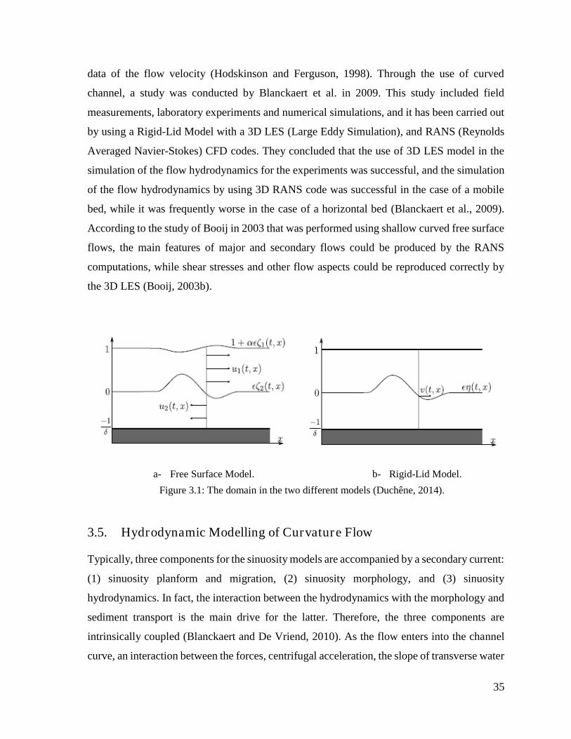
35
data of the flow velocity (Hodskinson and Ferguson, 1998). Through the use of curved
channel, a study was conducted by Blanckaert et al. in 2009. This study included field
measurements, laboratory experiments and numerical simulations, and it has been carried out
by using a Rigid-Lid Model with a 3D LES (Large Eddy Simulation), and RANS (Reynolds
Averaged Navier-Stokes) CFD codes. They concluded that the use of 3D LES model in the
simulation of the flow hydrodynamics for the experiments was successful, and the simulation
of the flow hydrodynamics by using 3D RANS code was successful in the case of a mobile
bed, while it was frequently worse in the case of a horizontal bed (Blanckaert et al., 2009).
According to the study of Booij in 2003 that was performed using shallow curved free surface
flows, the main features of major and secondary flows could be produced by the RANS
computations, while shear stresses and other flow aspects could be reproduced correctly by
the 3D LES (Booij, 2003b).
3.5. Hydrodynamic Modelling of Curvature Flow
Typically, three components for the sinuosity models are accompanied by a secondary current:
(1) sinuosity planform and migration, (2) sinuosity morphology, and (3) sinuosity
hydrodynamics. In fact, the interaction between the hydrodynamics with the morphology and
sediment transport is the main drive for the latter. Therefore, the three components are
intrinsically coupled (Blanckaert and De Vriend, 2010). As the flow enters into the channel
curve, an interaction between the forces, centrifugal acceleration, the slope of transverse water
a- Free Surface Model. b- Rigid-Lid Model.
Figure 3.1: The domain in the two different models (Duchêne, 2014).
36
surface, and bed shear stress occurs and produces a cross circulation as a result (Howard and
Chang, 1988). In order to include the effect of the secondary flow, the hydrodynamic
modelling of curvature flow could be mainly categorized into two categories; the linear model,
and nonlinear model. Also, linear closure sub models are generally used. The first order
disturbance process with the depth to curvature ratio, as a disturbance parameter, leads to these
sub models. In spite of the significant progress of the linear models in understanding and
revealing the dynamics of curvature, the omission of high curvature effects and validity
limitation to weak curvatures make them flawed. The straight flow profile of longitudinal
velocity in the vertical direction adoption is the main reason for the overestimation of the
linear model, thereby ignoring the feedback mechanism. As a result, it could be concluded
that the influences of the center region cell in a moderately to highly curved flow can only be
modelled if the deformation of the velocity profiles at the downstream is taken in
consideration. Also, the downstream velocity and the center-region cell feedback has to be
considered as well. In spite of the difficulty in coding and expensive computation for nonlinear
models, a number of nonlinear models have been suggested to overcome the linear approach’s
fundamental shortcomings. According to the previous studies, the linear model predictions for
narrow curves have been amended by Blanckaert and De Vriend by including a correction
factor. This factor includes the feedback between the velocity in the downstream and the
secondary circulation. In the sharp bends, the downstream velocity and boundary shear stress
should be modelled accurately in depth-integrated flow models. Thus, the so-called nonlinear
model was developed including these terms into the linear model formulation. To satisfy the
predictions in the river curves, 3D numerical models could be considered eligible for this.
These models depend on the consolidation of the three-dimensional flow features with the
complex spiral flow motion in the river bend. However, most of the 3D models suffer from
the large amounts of computational time and possible numerical instability (Song et al., 2012).
In this research, the secondary currents effect was examined on the hydraulic structures and
water surface elevation in a curved channel by developing a 3D finite element model of the
shallow water equations.
37
3.6. Mathematical Model
The conservation equations of mass, momentum and energy for incompressible flows will be
described generally in this part. First, a derivation to the equations in the most general form
should be done. The mathematical equations that exemplify the physical principles could be
extracted by applying the suitable fundamental physical principle into an appropriate model
of flow. The fluid flow has been modelled with infinitesimal control volume fixed in space
and the fluid moving through it. As a result, the equations are proposed in a differential
conservation form. It is important to recall the concept of the fundamental derivative in case
of switching from one form to another (Anderson, 1995):
𝑑
𝑑𝑡=
𝜕
𝜕𝑡+ (��. ∇) (3. 1)
Second, a suitable model for the fluid should be proposed; introduce the cases of interest in a
simple way such as ideal gas and Newtonian fluid.
3.7. Navier Stokes Equations
The conservation of mass (continuity) and momentum laws are used to describe the flow based
on the assumptions mentioned earlier. The Navier Stokes equations in the x, y and z directions
and the continuity equation that describes the flow are shown in equations below.
Momentum in x-direction;
𝜕
𝜕𝑡(𝜌𝑢) +
𝜕
𝜕𝑥(𝜌𝑢𝑢) +
𝜕
𝜕𝑦(𝜌𝑣𝑢) +
𝜕
𝜕𝑧(𝜌𝑤𝑢) = −
𝜕𝑃
𝜕𝑥+ 𝜇 (
𝜕2𝑢
𝜕𝑥2+
𝜕2𝑢
𝜕𝑦2+
𝜕2𝑢
𝜕𝑧2) (3.2)
Momentum in y-direction;
𝜕
𝜕𝑡(𝜌𝑣) +
𝜕
𝜕𝑥(𝜌𝑢𝑣) +
𝜕
𝜕𝑦(𝜌𝑣𝑣) +
𝜕
𝜕𝑧(𝜌𝑤𝑣) = −
𝜕𝑃
𝜕𝑦+ 𝜇 (
𝜕2𝑣
𝜕𝑥2+
𝜕2𝑣
𝜕𝑦2+
𝜕2𝑣
𝜕𝑧2) (3. 3)
Momentum in z-direction;
𝜕
𝜕𝑡(𝜌𝑤) +
𝜕
𝜕𝑥(𝜌𝑢𝑤) +
𝜕
𝜕𝑦(𝜌𝑣𝑤) +
𝜕
𝜕𝑧(𝜌𝑤𝑤) = −
𝜕𝑃
𝜕𝑧+ 𝜇 (
𝜕2𝑤
𝜕𝑥2+
𝜕2𝑤
𝜕𝑦2+
𝜕2𝑤
𝜕𝑧2) (3.4)
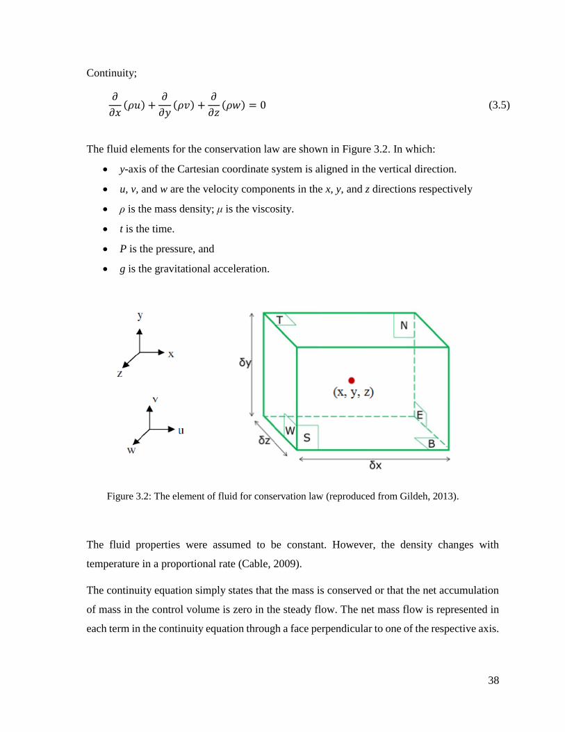
38
Continuity;
𝜕
𝜕𝑥(𝜌𝑢) +
𝜕
𝜕𝑦(𝜌𝑣) +
𝜕
𝜕𝑧(𝜌𝑤) = 0 (3.5)
The fluid elements for the conservation law are shown in Figure 3.2. In which:
y-axis of the Cartesian coordinate system is aligned in the vertical direction.
u, v, and w are the velocity components in the x, y, and z directions respectively
ρ is the mass density; μ is the viscosity.
t is the time.
P is the pressure, and
g is the gravitational acceleration.
The fluid properties were assumed to be constant. However, the density changes with
temperature in a proportional rate (Cable, 2009).
The continuity equation simply states that the mass is conserved or that the net accumulation
of mass in the control volume is zero in the steady flow. The net mass flow is represented in
each term in the continuity equation through a face perpendicular to one of the respective axis.
Figure 3.2: The element of fluid for conservation law (reproduced from Gildeh, 2013).
39
Equations (3.1) to (3.5) describe the flow distributions. Velocity can highly vary with time in
the turbulent flow. Many models have been studied and developed in order to predict turbulent
flow.
3.8. Discretization Approaches
The main purpose of derivation of the physical mathematical model is to manipulate it in an
appropriate form for computer calculations. Equation discretization is the first step in this
way. The discretization approach depends mainly on making a set of discrete algebraic
equations as one equation for every node. The value in the node should be in relation with
ones in the neighbour. Then, the numerical solution could be obtained from the simultaneous
gratification of all the equations in the set. The following is a discussion and presentation for
the most popular discretization techniques (Anderson, 1995).
3.8.1. Finite Volume Method (FVM)
This method depends on the integral form of the conservation equations. Basically, there are
finite volumes, which come from dividing the same domain. The centroids of these volumes
represent the calculation node. Boundaries between different volumes are defined by the grid
and should not be relating to any metrics. In terms of nodal values, the variable values of the
surface can be expressed by using interpolation. As long as surface integrals for volumes
sharing the same face are equal for both of them, this method is conservative. The shortcoming
of this method compared to FDM is that this method is more appropriate to the second order
schemes, and is more difficult for 3D simulations due to the three levels of approximation
introduced; interpolation, differentiation and integration. However, this method could be
considered as the most commonly used approach in fluid mechanics due to the physical
approach and the simplicity in understanding and implementing.
3.8.2. Finite Volume Method in OpenFOAM
OpenFOAM software, which is used in this thesis, is based on the FVM. The FVM is based
on conservation equations in the integral form as mentioned earlier. The integration should be
performed over a finite volume to get such equations. To clarify the ideas, the generic
conservation equation for a transported scalar Φ is shown in (3.6):
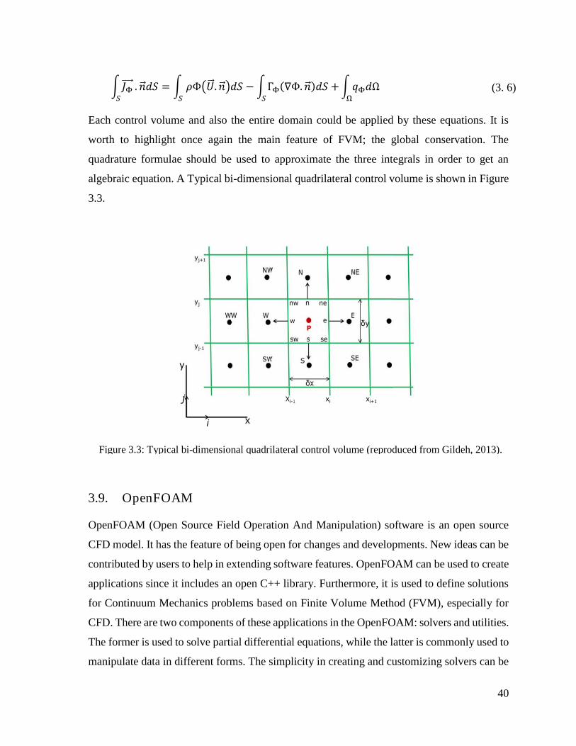
40
∫𝐽Φ
𝑆
. �� 𝑑𝑆 = ∫ 𝜌Φ(�� . �� )𝑑𝑆 − ∫ΓΦ(∇Φ. �� )𝑑𝑆 +
𝑆
𝑆
∫𝑞Φ𝑑Ω
Ω
(3. 6)
Each control volume and also the entire domain could be applied by these equations. It is
worth to highlight once again the main feature of FVM; the global conservation. The
quadrature formulae should be used to approximate the three integrals in order to get an
algebraic equation. A Typical bi-dimensional quadrilateral control volume is shown in Figure
3.3.
3.9. OpenFOAM
OpenFOAM (Open Source Field Operation And Manipulation) software is an open source
CFD model. It has the feature of being open for changes and developments. New ideas can be
contributed by users to help in extending software features. OpenFOAM can be used to create
applications since it includes an open C++ library. Furthermore, it is used to define solutions
for Continuum Mechanics problems based on Finite Volume Method (FVM), especially for
CFD. There are two components of these applications in the OpenFOAM: solvers and utilities.
The former is used to solve partial differential equations, while the latter is commonly used to
manipulate data in different forms. The simplicity in creating and customizing solvers can be
Figure 3.3: Typical bi-dimensional quadrilateral control volume (reproduced from Gildeh, 2013).
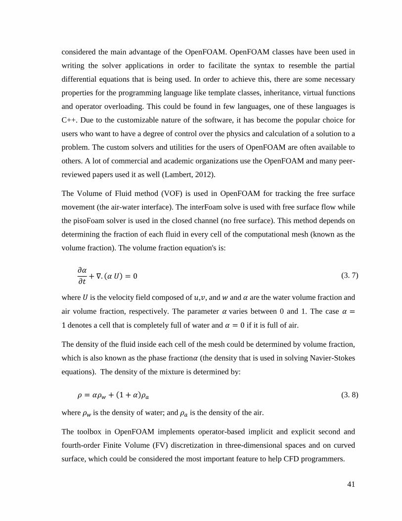
41
considered the main advantage of the OpenFOAM. OpenFOAM classes have been used in
writing the solver applications in order to facilitate the syntax to resemble the partial
differential equations that is being used. In order to achieve this, there are some necessary
properties for the programming language like template classes, inheritance, virtual functions
and operator overloading. This could be found in few languages, one of these languages is
C++. Due to the customizable nature of the software, it has become the popular choice for
users who want to have a degree of control over the physics and calculation of a solution to a
problem. The custom solvers and utilities for the users of OpenFOAM are often available to
others. A lot of commercial and academic organizations use the OpenFOAM and many peer-
reviewed papers used it as well (Lambert, 2012).
The Volume of Fluid method (VOF) is used in OpenFOAM for tracking the free surface
movement (the air-water interface). The interFoam solve is used with free surface flow while
the pisoFoam solver is used in the closed channel (no free surface). This method depends on
determining the fraction of each fluid in every cell of the computational mesh (known as the
volume fraction). The volume fraction equation's is:
𝜕𝛼
𝜕𝑡+ ∇. (𝛼 𝑈) = 0 (3. 7)
where 𝑈 is the velocity field composed of 𝑢,𝑣, and 𝑤 and 𝛼 are the water volume fraction and
air volume fraction, respectively. The parameter 𝛼 varies between 0 and 1. The case 𝛼 =
1 denotes a cell that is completely full of water and 𝛼 = 0 if it is full of air.
The density of the fluid inside each cell of the mesh could be determined by volume fraction,
which is also known as the phase fraction𝛼 (the density that is used in solving Navier-Stokes
equations). The density of the mixture is determined by:
𝜌 = 𝛼𝜌𝑤 + (1 + 𝛼)𝜌𝑎 (3. 8)
where 𝜌𝑤 is the density of water; and 𝜌𝑎 is the density of the air.
The toolbox in OpenFOAM implements operator-based implicit and explicit second and
fourth-order Finite Volume (FV) discretization in three-dimensional spaces and on curved
surface, which could be considered the most important feature to help CFD programmers.
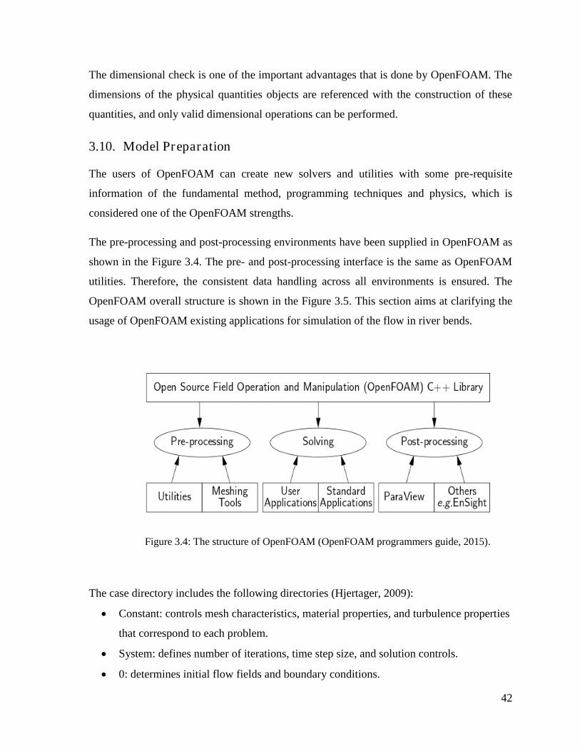
42
The dimensional check is one of the important advantages that is done by OpenFOAM. The
dimensions of the physical quantities objects are referenced with the construction of these
quantities, and only valid dimensional operations can be performed.
3.10. Model Preparation
The users of OpenFOAM can create new solvers and utilities with some pre-requisite
information of the fundamental method, programming techniques and physics, which is
considered one of the OpenFOAM strengths.
The pre-processing and post-processing environments have been supplied in OpenFOAM as
shown in the Figure 3.4. The pre- and post-processing interface is the same as OpenFOAM
utilities. Therefore, the consistent data handling across all environments is ensured. The
OpenFOAM overall structure is shown in the Figure 3.5. This section aims at clarifying the
usage of OpenFOAM existing applications for simulation of the flow in river bends.
The case directory includes the following directories (Hjertager, 2009):
Constant: controls mesh characteristics, material properties, and turbulence properties
that correspond to each problem.
System: defines number of iterations, time step size, and solution controls.
0: determines initial flow fields and boundary conditions.
Figure 3.4: The structure of OpenFOAM (OpenFOAM programmers guide, 2015).
43
The case structure is shown in the Figure 3.5.
As mentioned earlier, there are several different solvers within the OpenFOAM toolbox that
are designed to solve various specific problems (Poungkrajorn, 2015). Two solvers have been
selected to solve the problem regarding the experiment in this research:
InterFoam: is a transient solver for incompressible flow that is used with Free Surface Model.
PisoFoam: is a transient solver for incompressible flow that is used with Rigid-Lid Model.
3.10.1. Implementation of the Solvers
3.10.1.1. InterFoam Solver
Free surface flows are characterized by a high interaction between air and water. Some of
these characteristics can be reproduced by the interFoam solver of OpenFOAM, which is a
multiphase solver.
3.10.1.2. PisoFoam Solver
PisoFoam is a transient solver for incompressible fluid flows and it works for both laminar
Figure 3.5: OpenFOAM case structure (Hjertager, 2009).
44
and turbulent conditions. PISO algorithm is the base of pisoFoam, which stands for Pressure
Implicit with Splitting of Operators. Basically, pisoFoam is a process of pressure-velocity
calculation that includes one predictor step and two corrector steps. Momentum equations are
used in the predictor step for solving an intermediate pressure field, which is the concept of
the SIMPLE algorithm. The correcting and ensuring the relevant parameters is done by two
corrector steps in a way to satisfy the momentum and continuity equations (Versteeg and
Malalasekera, 2007). Therefore, pisoFoam also could be considered as an extension of the
SIMPLE algorithm by adding corrector steps in order to ensure the calculated values
(Poungkrajorn, 2015).
3.11. Turbulence Modelling
Turbulent flow is one of the flow cases in fluid dynamics. It is characterized by a random
motion of the fluid within a flow domain. On the other hand, laminar flow, non-turbulent or
streamlines, is the flow where the fluid flows in parallel layers with no disruption between the
layers. In order to indicate the type of the flow whether it is considered laminar or turbulent,
Reynolds Number could be used (Cable, 2009).
Turbulent flow can be characterized by several characteristic features such as (Davidson,
2015):
Irregularity: The turbulent flow is irregular, random and chaotic.
Diffusivity: The diffusivity increases in the turbulent flow.
Large Reynolds Number: Turbulent flow occurs at high Reynolds number.
Three-Dimensional: The turbulent flow is always three-dimensional. Nevertheless, the
flow can be treated as two-dimensional when the equations are time averaged.
Dissipation: Turbulent flow is dissipative. In other words, the kinetic energy is
transformed into internal energy in the small eddies.
Continuum: The turbulent scales are small in the flow although they are much larger
than the molecular scale. Also, the flow could be treated as a continuum.
The decomposition for the instantaneous variables such as the components of velocity and
pressure into a mean value and fluctuating value is preferable when the flow is turbulent as
shown in equation below (Davidson, 2015).
45
𝑈𝑖 = ��𝑖 + 𝑢𝑖 (3. 9)
𝑃 = �� + 𝑝 (3. 10)
The reason behind the variables decomposition is that in measuring flow quantities the mean
values are commonly more interesting than the time histories.
In addition, solving the Navier-Stokes equation numerically requires a very fine grid to solve
all turbulent scales. The fine resolution in time is required as well because the turbulent flow
is always unsteady.
The equation of continuity and Navier-Stokes equation can be written as shown below:
𝜕𝑝
𝜕𝑡+ (𝜌𝑈𝑖) = 0 (3. 11)
𝜕𝑝𝑈𝑖
𝜕𝑡+ (𝜌𝑈𝑖𝑈𝑗)𝑗
= −𝑃𝑖 + [𝜇 (𝑈𝑖,𝑗 + 𝑈𝑗,𝑖 −2
3𝜎𝑖,𝑗𝑈𝑘,𝑘)]
𝑗 (3. 12)
where (.), j indicates the derivation with respect to xj.
In order to deal with the incompressible flow, the last term on the right hand side of Equation
(3. 12) is neglected. So that the equation will be:
𝜕𝑝𝑈𝑖
𝜕𝑡+ (𝜌𝑈𝑖𝑈𝑗)𝑗
= −𝑃𝑖 + [𝜇(𝑈𝑖,𝑗 + 𝑈𝑗,𝑖)]𝑗 (3. 13)
The following equations are obtained after time averaging of the continuity and Navier-Stokes
equations.
𝜕𝑝
𝜕𝑡+ (𝜌��𝑖),𝑖 = 0 (3. 14)
𝜕𝑝��𝑖
𝜕𝑡+ (𝜌��𝑖��𝑗)𝑗
= −��𝑖 + [𝜇(��𝑖,𝑗 + ��𝑗,𝑖) − 𝜌𝑢𝑖𝑢𝑗 ]𝑗 (3. 15)
where 𝑢𝑖𝑢𝑗 is the Reynolds stress tensor. The above equations are called Reynolds-Averaged
Navier Stokes (RANS) equations. Different turbulence models could be used to perform the
estimation of Reynolds stress tensor as described below.
46
3.11.1. Various Turbulence Models
Turbulence models have been developed in different types by solving the Navier Stokes
equations and Reynolds-Averaged Navier Stokes (RANS) based on modelling approach that
reduces the computational efforts and resources using time averaging the flow quantities for
a whole range of scales of turbulence that are being modeled (Cable, 2009). Several models,
that are included in RANS turbulence models, have been developed in increasing order of
complexity, ability to model the turbulence, and cost in terms of computational work (CPU
time) Such as (Davidson, 2015):
Algebraic (zero equation) models: mixing length (first order model);
One equation models: 𝑘‐model, 𝜇𝑡‐model, Spalart-Allmaras (first order model);
Two equation models: 𝑘‐ 휀, 𝑘‐ 𝑘𝑙, 𝑘‐𝜔2, low Re 𝑘‐ 휀 (first order model);
Algebraic stress models: ASM (second order model); and
Reynolds stress models: RSM (second order model).
A brief explanation for each group of the turbulence models is shown below:
I. Algebraic models: Turbulent viscosity or even often called eddy viscosity is computed
by an algebraic equation. Eddy viscosity models are based on a turbulent (eddy)
viscosity.
II. One-equation models: The turbulent quantity (commonly the turbulent kinetic
energy), for this kind of models is obtained from a transport equation. In addition, an
algebraic expression is solved for a second turbulent quantity, commonly a scale of
turbulent length. Boussinesq assumption is usually used for calculating the turbulence
viscosity.
III. Two-equation models: These models lie within the class of eddy viscosity models. In
order to describe the transport of two scalars, two transport equations are derived; the
turbulent kinetic energy 𝑘 and its dissipation 휀. Then, the assumption that relates the
Reynolds stress tensor to the velocity gradients and an eddy viscosity is used to
compute the Reynolds stress tensor. The eddy viscosity is gotten from the two
transported scalars.
47
IV. Reynolds stress models: In this case, the derivation of the transport equation is used
for the Reynolds tensor. In order to determine the length scale of the turbulence, one
transport equation should be added, commonly the dissipation 휀 equation is used.
The k – ε model is widely used because of several features such as; the robustness and
reasonable accuracy that it provided for a large number of turbulent flows (Cable, 2009).
3.11.1.1. Boussinesq Assumption
Boussinesq assumption could be described as the relationship between the Reynolds stresses
and the velocity gradients via the turbulence viscosity. It is written as:
[𝜇(��𝑖,𝑗 + ��𝑗,𝑖) − 𝜌𝑢𝑖𝑢𝑗 ]𝑗= [(𝜇 + 𝜇𝑡)(��𝑖,𝑗 + ��𝑗,𝑖)],𝑗 (3. 16)
which gives:
𝜌𝑢𝑖𝑢𝑗 = −𝜇𝑡(��𝑖,𝑗 + ��𝑗,𝑖),𝑗 (3. 17)
or,
𝜌𝑢𝑖𝑢𝑗 = −𝜇𝑡(��𝑖,𝑗 + ��𝑗,𝑖) +2
3𝛿𝑖𝑗𝜌𝑘 (3. 18)
where the last term is equal to zero in incompressible flows.
3.11.1.2. Algebraic Models
An expression for the turbulent viscosity is required in eddy viscosity models (𝜇𝑡 = 𝜌𝜈𝑡). The
dimension of 𝜈𝑡 is [𝑚2/𝑠]. A scale of turbulent velocity multiplied with a scale of turbulent
length gives the right dimension such that:
𝑣𝑡 ∝ 𝑢 ℓ (3. 19)
where 𝑢 and ℓ are the characteristic for the large turbulent scales.
This is considered reasonable since most of the transport by turbulent diffusion lies under the
responsibility of these scales. The velocity gradient is used as a velocity scale in the algebraic
turbulence model. Also, some of the physical length is used as the length scale. In boundary
layer-type of flow, the dimension of 𝜈𝑡 is:
48
𝑣𝑡 = ℓ𝑚𝑖𝑥2 |
𝜕𝑈
𝜕𝑦| (3. 20)
where 𝑦 is the coordinate normal to the wall; ℓ𝑚𝑖𝑥 is the length of mixing; and the model is
named as the mixing length model. This model is hardly used anymore since it is an old one.
The only problem in this model is that ℓ𝑚𝑖𝑥 is unknown and should be determined. More
modern algebraic models are the Baldwin-Lomax model (Baldwin and Lomax, 1978) and the
Cebeci-Smith model (Cebeci and Smith, 1974) which are commonly used in aerodynamics
when the flow is computed around aeroplanes, airfoils and in other situations.
3.11.1.3. One Equation Models
The transport equation is mostly solved for the turbulent kinetic energy in one equation
models. An algebraic expression is often used for the unknown turbulent length scale, which
should always be given. For instance, the length scale can be taken as commensurate to the
boundary layer thickness, the width of a jet or a wake. Due to the impossibility of this model
in finding a common expression for an algebraic length scale, it is not appropriate to general
flows, which is considered the main shortcoming for this type. Despite that, several
suggestions were made where the scale of turbulent length is computed in a more common
way.
3.11.1.4. Two-Equation Turbulence Models
Turbulent flows include two-equation models; the Standard k-ε model and the Modeled 𝑘
Equation.
The k-ε model is one of the turbulence models that is used in Computational Fluid Dynamics
(CFD). It is mainly used for developed and general turbulence. The model allows for the
impact of transport of turbulence properties by convection, diffusion, and the production and
destruction of turbulence. Since it is a two equation model, the description of turbulence is
given by means of two transport equations (PDEs); the turbulent kinetic energy (𝑘), and the
rate of dissipation of turbulent kinetic energy (휀). The turbulent viscosity is isotropic and the
main presumption of this model is considered according to Versteeg and Malalasekera (2007).
Accordingly, the ratio between Reynolds stress and mean rate of deformation is the same at
49
all directions. Nevertheless, the inaccurate predictions makes this assumption failing in many
complex flows (Tawekal, 2015).
The evaluation for the standard k-ε according to Versteeg and Malalasekera can be
summarized as follows (2007)
Advantages
o It is considered the simplest turbulence model because there is no need to
specify the initial and/or boundary conditions;
o a very good performance was given by this model, especially in many
industrially relevant flows;
o The model is well established; and It is the most extensively certified
turbulence model.
Disadvantages
o It could be considered expensive comparing with other turbulence models
like mixing length model; and
o The performance of the model could be considered poor in assortment of
significant cases such as:
Unconfined flows;
Flows with large extra strains;
Rotating flows; and
Flows driven by anisotropy of normal Reynolds stresses.
Further details for all the turbulence models are provided in the Appendix A.
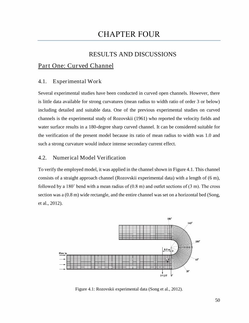
50
CHAPTER FOUR
4. RESULTS AND DISCUSSIONS
Part One: Curved Channel
4.1. Experimental Work
Several experimental studies have been conducted in curved open channels. However, there
is little data available for strong curvatures (mean radius to width ratio of order 3 or below)
including detailed and suitable data. One of the previous experimental studies on curved
channels is the experimental study of Rozovskii (1961) who reported the velocity fields and
water surface results in a 180-degree sharp curved channel. It can be considered suitable for
the verification of the present model because its ratio of mean radius to width was 1.0 and
such a strong curvature would induce intense secondary current effect.
4.2. Numerical Model Verification
To verify the employed model, it was applied in the channel shown in Figure 4.1. This channel
consists of a straight approach channel (Rozovskii experimental data) with a length of (6 m),
followed by a 180˚ bend with a mean radius of (0.8 m) and outlet sections of (3 m). The cross
section was a (0.8 m) wide rectangle, and the entire channel was set on a horizontal bed (Song,
et al., 2012).
Figure 4.1: Rozovskii experimental data (Song et al., 2012).
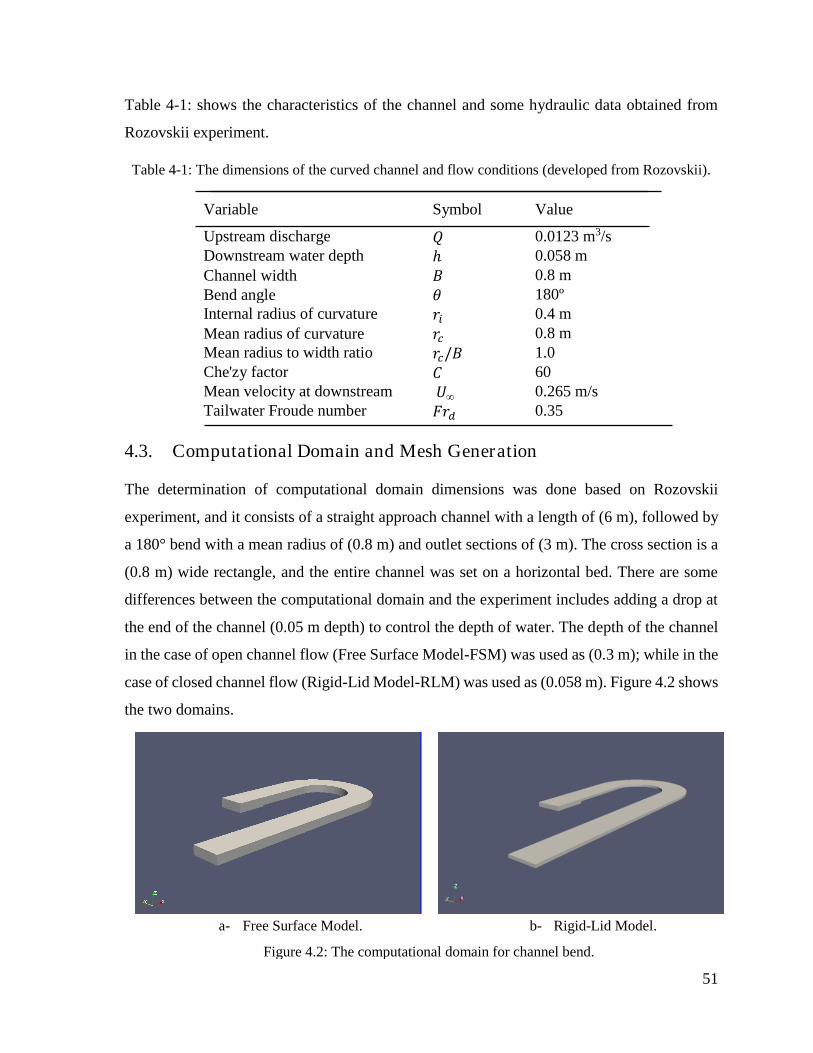
51
Table 4-1: shows the characteristics of the channel and some hydraulic data obtained from
Rozovskii experiment.
Table 4-1: The dimensions of the curved channel and flow conditions (developed from Rozovskii).
Variable Symbol Value
Upstream discharge 𝑄 0.0123 m3/s
Downstream water depth ℎ 0.058 m
Channel width 𝐵 0.8 m
Bend angle 𝜃 180º
Internal radius of curvature 𝑟𝑖 0.4 m
Mean radius of curvature 𝑟𝑐 0.8 m
Mean radius to width ratio 𝑟𝑐/𝐵 1.0
Che'zy factor 𝐶 60
Mean velocity at downstream 𝑈∞ 0.265 m/s
Tailwater Froude number 𝐹𝑟𝑑 0.35
4.3. Computational Domain and Mesh Generation
The determination of computational domain dimensions was done based on Rozovskii
experiment, and it consists of a straight approach channel with a length of (6 m), followed by
a 180° bend with a mean radius of (0.8 m) and outlet sections of (3 m). The cross section is a
(0.8 m) wide rectangle, and the entire channel was set on a horizontal bed. There are some
differences between the computational domain and the experiment includes adding a drop at
the end of the channel (0.05 m depth) to control the depth of water. The depth of the channel
in the case of open channel flow (Free Surface Model-FSM) was used as (0.3 m); while in the
case of closed channel flow (Rigid-Lid Model-RLM) was used as (0.058 m). Figure 4.2 shows
the two domains.
a- Free Surface Model. b- Rigid-Lid Model.
Figure 4.2: The computational domain for channel bend.
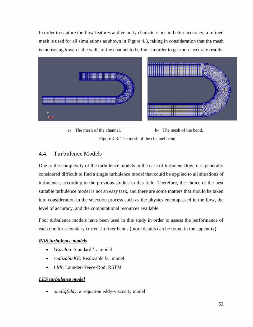
52
In order to capture the flow features and velocity characteristics in better accuracy, a refined
mesh is used for all simulations as shown in Figure 4.3, taking in consideration that the mesh
is increasing towards the walls of the channel to be finer in order to get more accurate results.
4.4. Turbulence Models
Due to the complexity of the turbulence models in the case of turbulent flow, it is generally
considered difficult to find a single turbulence model that could be applied to all situations of
turbulence, according to the previous studies in this field. Therefore, the choice of the best
suitable turbulence model is not an easy task, and there are some matters that should be taken
into consideration in the selection process such as the physics encompassed in the flow, the
level of accuracy, and the computational resources available.
Four turbulence models have been used in this study in order to assess the performance of
each one for secondary current in river bends (more details can be found in the appendix):
RAS turbulence models
kEpsilon: Standard k-ε model
realizableKE: Realizable k-ε model
LRR: Launder-Reece-Rodi RSTM
LES turbulence model
oneEqEddy: k -equation eddy-viscosity model
a- The mesh of the channel. b- The mesh of the bend.
Figure 4.3: The mesh of the channel bend.
53
4.5. The Numerical Simulations
The simulations in this study was done by using OpenFOAM (OPEN Field Operation And
Manipulation) which is an open source CFD program written mainly in C++. A number of
solvers come with this program, and each one of these solvers is designed for solving a specific
fluid mechanics problem. Also, there are utilities to perform data manipulation.
Basically, OpenFOAM uses the Finite Volume Method, FVM, and it includes a lot of
numerical schemes that are implemented both for time and space integration. Two solvers
were used in this study, the first one is interFoam solver which has been used for
incompressible and turbulent flows in open channel flow (Free Surface Model), and the other
one is pisoFoam solver which has been used also for incompressible and turbulent flow but in
closed channel cases (Rigid-Lid Model).
4.6. Initial and Boundary Conditions
In the domain of curved channel, there are four types of boundaries: the inlet and the outlet of
the channel, the walls (including side walls and bottom), and the surface of the channel
(atmosphere). There are one or more faces in each of these boundaries. It is necessary to
determine the initial and boundary conditions for each type of these boundaries before running
the simulation. A summary of the boundary conditions of each type of boundaries is presented
below:
Velocity:
The inlet boundaries of the velocity have been chosen as a fixedValue condition, while
the outlet boundaries of the velocity were set as a zeroGradient which means (the
normal gradient of velocity is zero). The boundary conditions of the side walls and
lower walls were specified as a fixedValue conditions with a uniform value of (0, 0,
0), which means that no-slip velocity condition is assumed at the walls and the velocity
at the walls is zero. For the top of the channel (atmosphere), the boundary condition
was determined as a zeroGradient when using the solver interFoam, and a
symmetryPlane when using the solver pisoFoam.
Pressure:
The boundary conditions of the pressure were set as a zeroGradient except for the
54
atmosphere, where the pressure was specified as a totalPressure with zero value for
the case of using the interFoam solver, and a symmetryPlane for the case of using the
pisoFoam solver.
Turbulent kinetic energy (𝒌):
According to Huai et al. (2010), k=0.06u2, where k= Turbulent kinetic energy, and u
= the mean velocity. The boundary conditions of the turbulent kinetic energy were
determined as follows: fixedValue at the inlet with the value of k as calculated from
the above equation, zeroGradient at outlet and the atmosphere, and finally the
wallFunction (kqRwallFunction) has been used for the side and lower walls which
provides a suitable condition for 𝑘 fields for the case of Reynolds number flow. In the
case of using the solver pisoFoam instead of interFoam, the only difference is that the
boundary condition of the atmosphere changes to symmetryPlane instead of
zeroGradient.
Rate of kinetic energy dissipation (ε):
According to Huai et al. (2010), ε=0.06u3/D, where ε= the rate of dissipation, u = the
mean velocity, and D= the depth of water. The boundary conditions of the rate of
dissipation or epsilon were specified as follows: fixedValue at the inlet with the value
of ε as calculated from the above equation, zeroGradient at the outlet and the
atmosphere, and finally the wallFunction (epsilonwallFunction) has been used for the
side and lower walls which provides a turbulence dissipation wall function condition
for high Reynolds numbers in turbulent flow cases. In the case of using the solver
pisoFoam instead of interFoam, the only difference is that the boundary condition of
the atmosphere changes to be symmetryPlane instead of zeroGradient.
Turbulent viscosity:
The boundary conditions of the turbulent viscosity have been chosen as a zeroGradient
for the inlet, outlet, and atmosphere. One of the wallFunctions called
(nutWallFunction) was chosen for the side and lower walls to determine the boundary
condition of the turbulent viscosity with a zero uniform value. In the case of using the
solver pisoFoam instead of interFoam, the only difference is that the boundary
condition of the atmosphere changes to be symmetryPlane instead of zeroGradient.
55
Kinematic viscosity (SGS) for LES model:
Same as the turbulent viscosity, all the boundary conditions were used as a
zeroGradient except for the side and lower walls were also one of the wallFunctions
was used called (nutkWallFunction) with a zero uniform value. In the case of using
the solver pisoFoam instead of interFoam, the only difference is that the boundary
condition of the atmosphere changes to be symmetryPlane instead of zeroGradient.
Reynolds stress (R) for LRR model:
The boundary conditions for the Reynolds stress was determined as a fixedValue for
the inlet with a zero uniform value, and zeroGradient for the outlet and the
atmosphere, while the wallFunction (kqRwallFunction) has been used for the side and
lower walls with a zero uniform value. In the case of using the solver pisoFoam instead
of interFoam, the only difference is that the boundary condition of the atmosphere
changes to be symmetryPlane instead of zeroGradient.
4.7. Results and Discussions
In order to understand the behaviour of the flow in channel bends, some turbulence models
were studied in this research. An evaluation for each model will be done based on velocity
parameters. The results of the velocities across dimensional channel width that obtained from
these models will be compared with Rozovskii experimental data (Rozovskii 1961). In
addition, three-dimensional velocity components will be studied to highlight the reasons
behind the variation in these velocities. Finally, each model will be evaluated depending on
the results obtained from simulation outputs to choose the best one for each case.
4.7.1. Free Surface Model
As mentioned previously, the Free Surface Model takes in consideration both the water and
the air in the simulation of the channel. A horizontal section was taken on the depth (0.242m)
from the top of the channel to examine the characteristics of water flow separately at channel
curve. Thus, the total depth of the channel is (𝐷𝑡 = 0.3 𝑚), and the depth of flow after the
steady state is (𝐷𝑓 = 0.058 𝑚), which is same as the depth of flow in the experiment
(0.058m). Figures (4-4) through (4-7) below illustrate the distribution of the velocity and the
depth of water for the channel at time zero and 300 seconds for standard k-ε, LRR, realizable
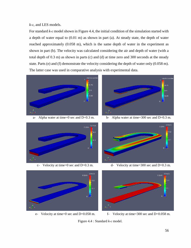
56
k-ε, and LES models.
For standard k-ε model shown in Figure 4.4, the initial condition of the simulation started with
a depth of water equal to (0.01 m) as shown in part (a). At steady state, the depth of water
reached approximately (0.058 m), which is the same depth of water in the experiment as
shown in part (b). The velocity was calculated considering the air and depth of water (with a
total depth of 0.3 m) as shown in parts (c) and (d) at time zero and 300 seconds at the steady
state. Parts (e) and (f) demonstrate the velocity considering the depth of water only (0.058 m).
The latter case was used in comparative analysis with experimental data.
a- Alpha water at time=0 sec and D=0.3 m. b- Alpha water at time=300 sec and D=0.3 m.
c- Velocity at time=0 sec and D=0.3 m. d- Velocity at time=300 sec and D=0.3 m.
e- Velocity at time=0 sec and D=0.058 m. f- Velocity at time=300 sec and D=0.058 m.
Figure 4.4 : Standard k-ε model.
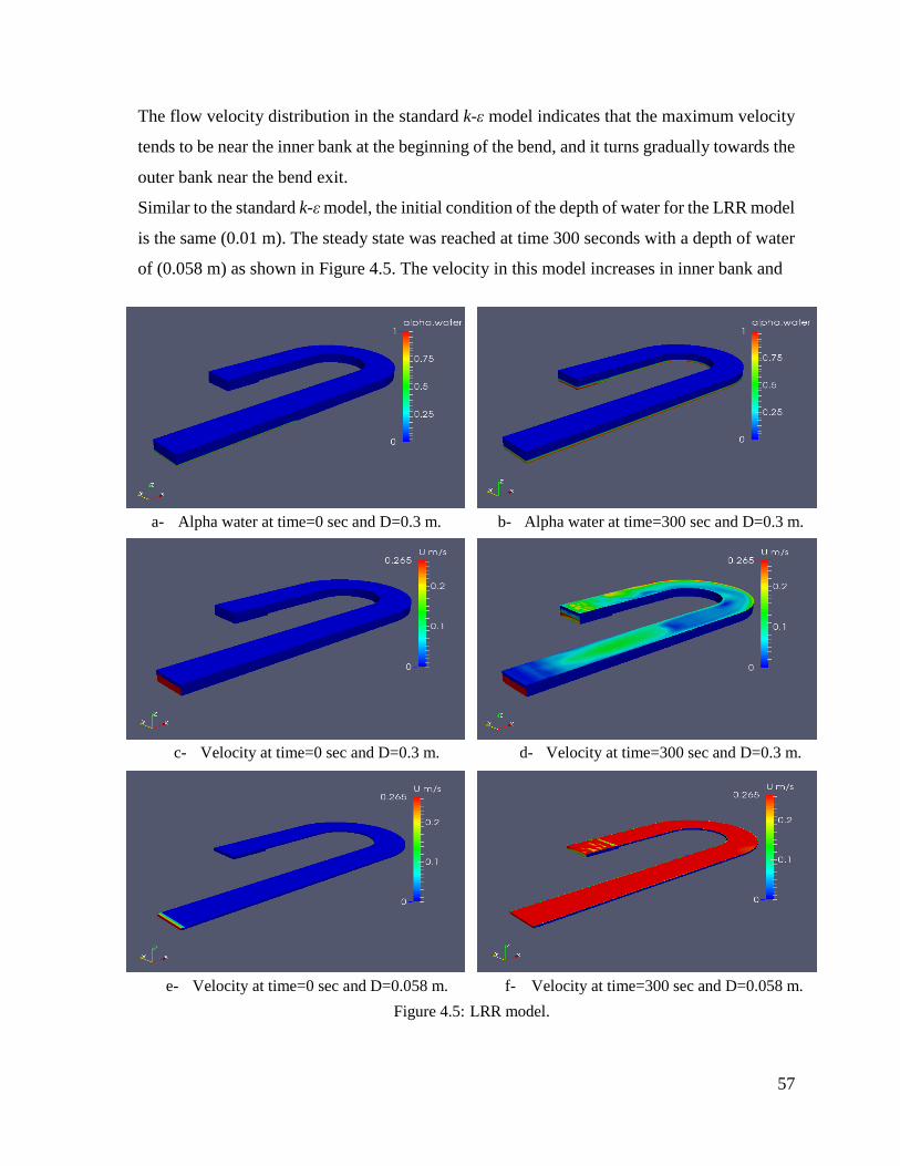
57
The flow velocity distribution in the standard k-ε model indicates that the maximum velocity
tends to be near the inner bank at the beginning of the bend, and it turns gradually towards the
outer bank near the bend exit.
Similar to the standard k-ε model, the initial condition of the depth of water for the LRR model
is the same (0.01 m). The steady state was reached at time 300 seconds with a depth of water
of (0.058 m) as shown in Figure 4.5. The velocity in this model increases in inner bank and
a- Alpha water at time=0 sec and D=0.3 m. b- Alpha water at time=300 sec and D=0.3 m.
c- Velocity at time=0 sec and D=0.3 m. d- Velocity at time=300 sec and D=0.3 m.
e- Velocity at time=0 sec and D=0.058 m. f- Velocity at time=300 sec and D=0.058 m.
Figure 4.5: LRR model.
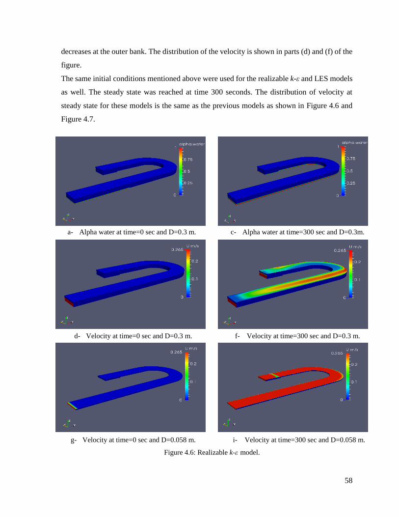
58
decreases at the outer bank. The distribution of the velocity is shown in parts (d) and (f) of the
figure.
The same initial conditions mentioned above were used for the realizable k-ε and LES models
as well. The steady state was reached at time 300 seconds. The distribution of velocity at
steady state for these models is the same as the previous models as shown in Figure 4.6 and
Figure 4.7.
a- Alpha water at time=0 sec and D=0.3 m. b- c- Alpha water at time=300 sec and D=0.3m.
d- Velocity at time=0 sec and D=0.3 m. e- f- Velocity at time=300 sec and D=0.3 m.
g- Velocity at time=0 sec and D=0.058 m. h- i- Velocity at time=300 sec and D=0.058 m.
Figure 4.6: Realizable k-ε model.
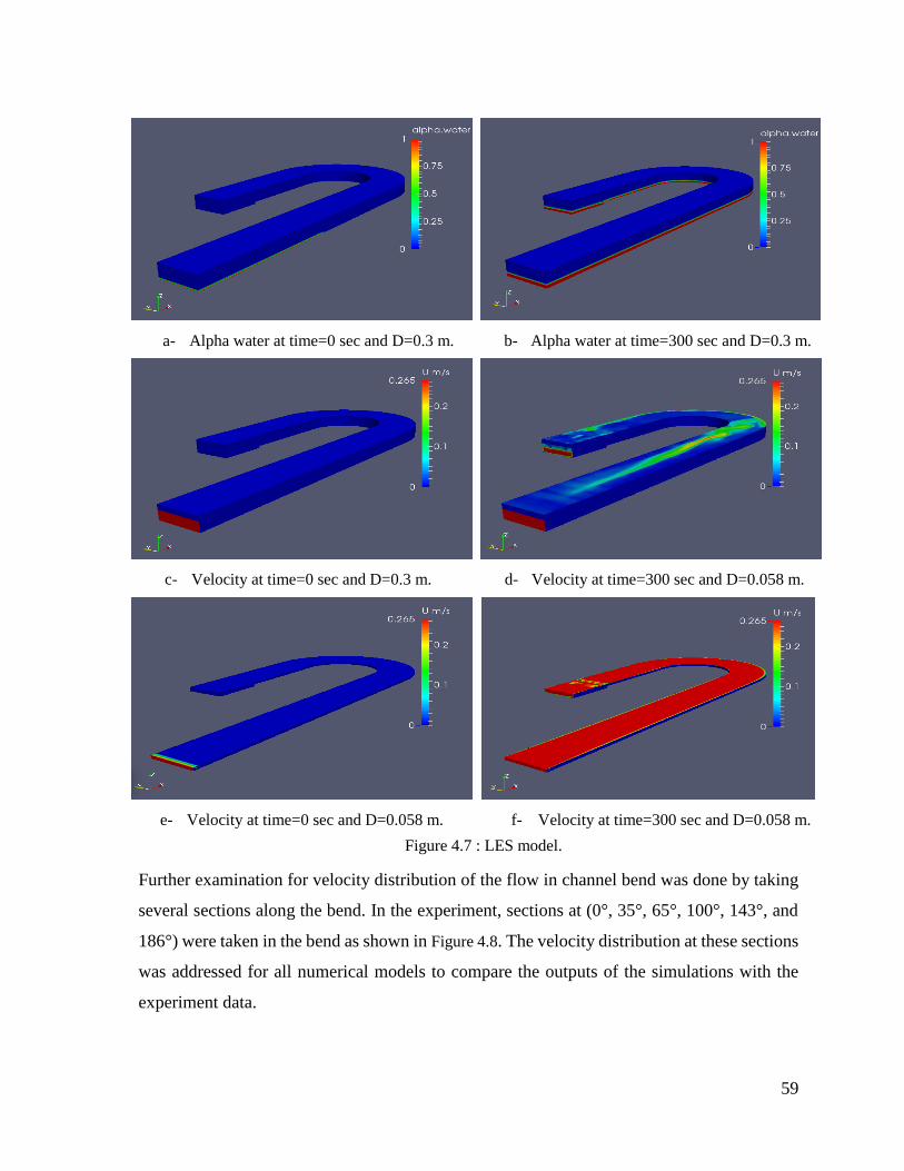
59
Further examination for velocity distribution of the flow in channel bend was done by taking
several sections along the bend. In the experiment, sections at (0°, 35°, 65°, 100°, 143°, and
186°) were taken in the bend as shown in Figure 4.8. The velocity distribution at these sections
was addressed for all numerical models to compare the outputs of the simulations with the
experiment data.
a- Alpha water at time=0 sec and D=0.3 m. b- Alpha water at time=300 sec and D=0.3 m.
c- Velocity at time=0 sec and D=0.3 m. d- Velocity at time=300 sec and D=0.058 m.
e- Velocity at time=0 sec and D=0.058 m. f- Velocity at time=300 sec and D=0.058 m.
Figure 4.7 : LES model.
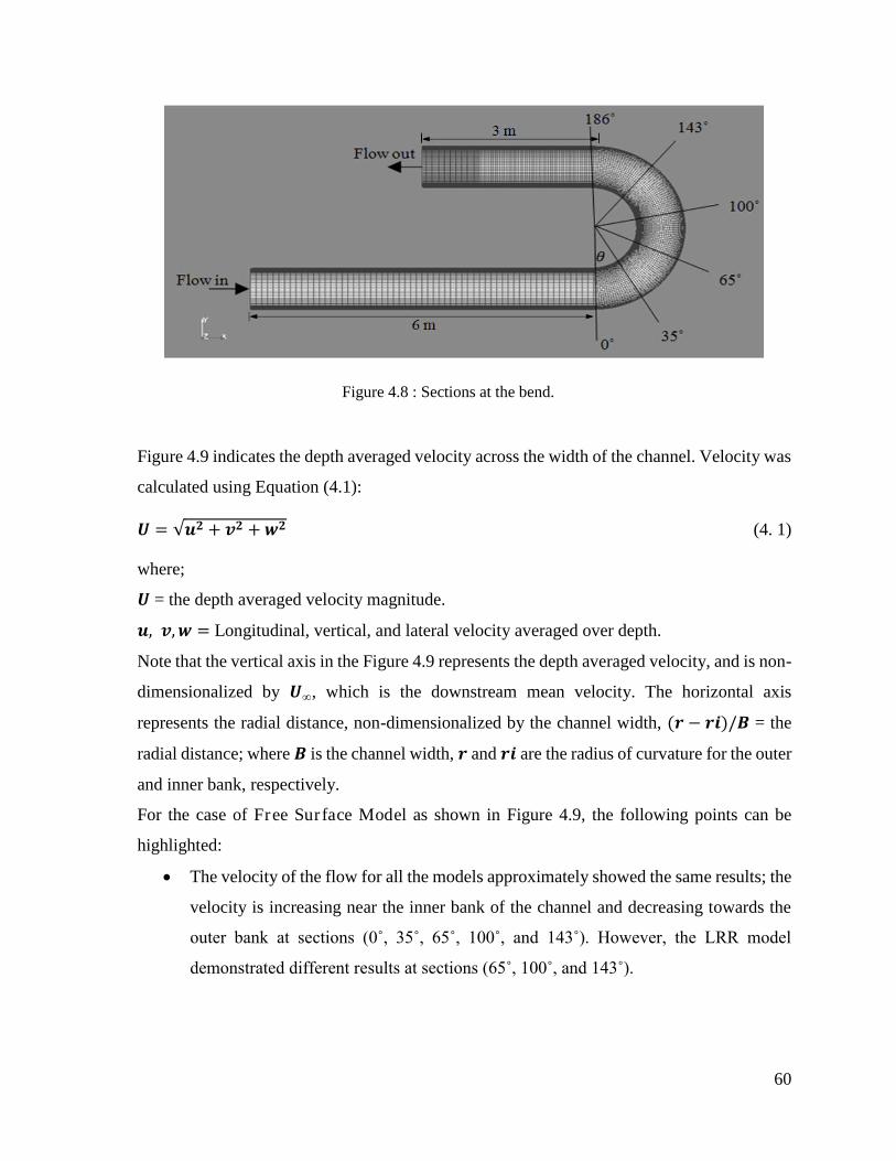
60
Figure 4.8 : Sections at the bend.
Figure 4.9 indicates the depth averaged velocity across the width of the channel. Velocity was
calculated using Equation (4.1):
𝑼 = √𝒖𝟐 + 𝒗𝟐 + 𝒘𝟐 (4. 1)
where;
𝑼 = the depth averaged velocity magnitude.
𝒖, 𝒗,𝒘 = Longitudinal, vertical, and lateral velocity averaged over depth.
Note that the vertical axis in the Figure 4.9 represents the depth averaged velocity, and is non-
dimensionalized by 𝑼∞, which is the downstream mean velocity. The horizontal axis
represents the radial distance, non-dimensionalized by the channel width, (𝒓 − 𝒓𝒊)/𝑩 = the
radial distance; where 𝑩 is the channel width, 𝒓 and 𝒓𝒊 are the radius of curvature for the outer
and inner bank, respectively.
For the case of Free Surface Model as shown in Figure 4.9, the following points can be
highlighted:
The velocity of the flow for all the models approximately showed the same results; the
velocity is increasing near the inner bank of the channel and decreasing towards the
outer bank at sections (0˚, 35˚, 65˚, 100˚, and 143˚). However, the LRR model
demonstrated different results at sections (65˚, 100˚, and 143˚).
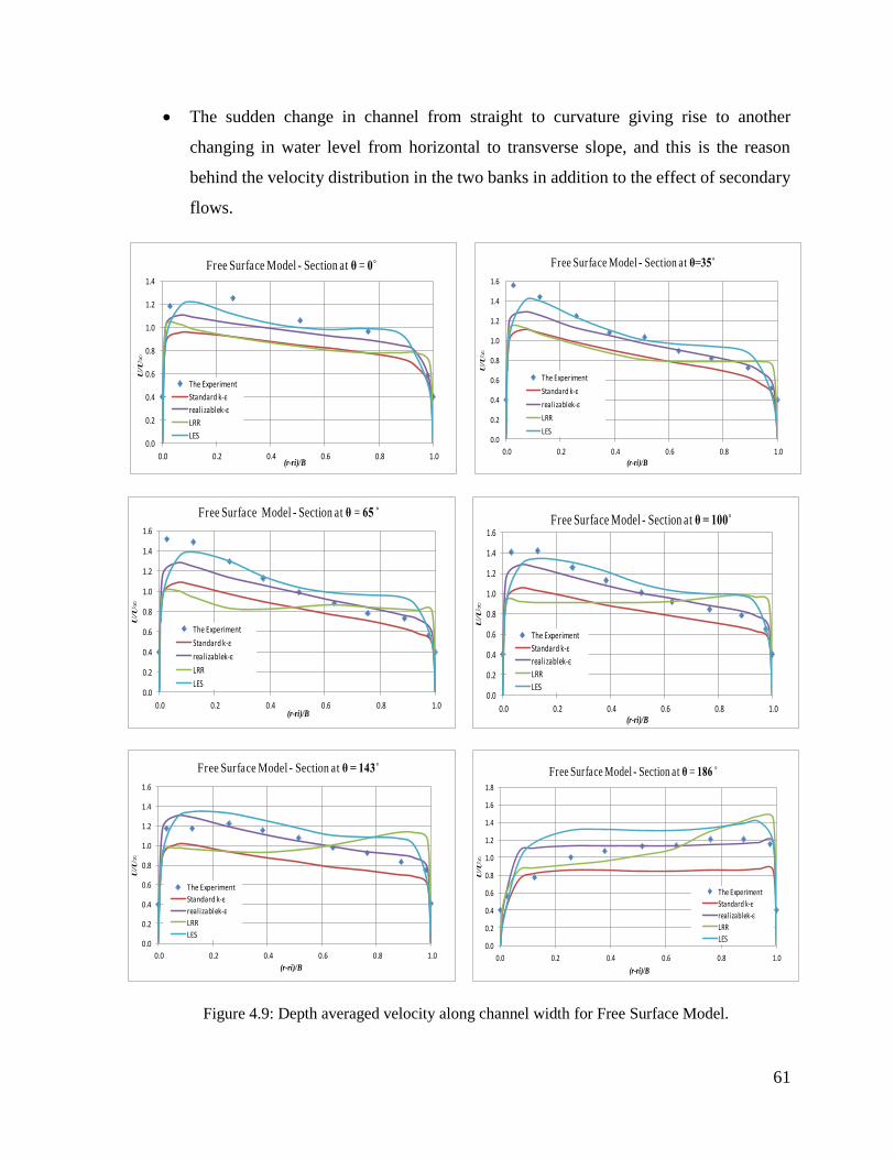
61
The sudden change in channel from straight to curvature giving rise to another
changing in water level from horizontal to transverse slope, and this is the reason
behind the velocity distribution in the two banks in addition to the effect of secondary
flows.
Figure 4.9: Depth averaged velocity along channel width for Free Surface Model.
0.0
0.2
0.4
0.6
0.8
1.0
1.2
1.4
0.0 0.2 0.4 0.6 0.8 1.0
U/U
∞
(r-ri)/B
Free Surface Model - Section at θ = 0˚
The Experiment
Standard k-ε
realizablek-ε
LRR
LES 0.0
0.2
0.4
0.6
0.8
1.0
1.2
1.4
1.6
0.0 0.2 0.4 0.6 0.8 1.0
U/U
∞
(r-ri)/B
Free Surface Model - Section at θ=35˚
The Experiment
Standard k-ε
realizablek-ε
LRR
LES
0.0
0.2
0.4
0.6
0.8
1.0
1.2
1.4
1.6
0.0 0.2 0.4 0.6 0.8 1.0
U/U
∞
(r-ri)/B
Free Surface Model - Section at θ = 65
The Experiment
Standard k-ε
realizablek-ε
LRR
LES
0.0
0.2
0.4
0.6
0.8
1.0
1.2
1.4
1.6
0.0 0.2 0.4 0.6 0.8 1.0
U/U
∞
(r-ri)/B
Free Surface Model - Section at θ = 100˚
The Experiment
Standard k-ε
realizablek-ε
LRR
LES
0.0
0.2
0.4
0.6
0.8
1.0
1.2
1.4
1.6
0.0 0.2 0.4 0.6 0.8 1.0
U/U
∞
(r-ri)/B
Free Surface Model - Section at θ = 143˚
The Experiment
Standard k-ε
realizablek-ε
LRR
LES
0.0
0.2
0.4
0.6
0.8
1.0
1.2
1.4
1.6
1.8
0.0 0.2 0.4 0.6 0.8 1.0
U/U
∞
(r-ri)/B
Free Surface Model - Section at θ = 186
The Experiment
Standard k-ε
realizablek-ε
LRR
LES
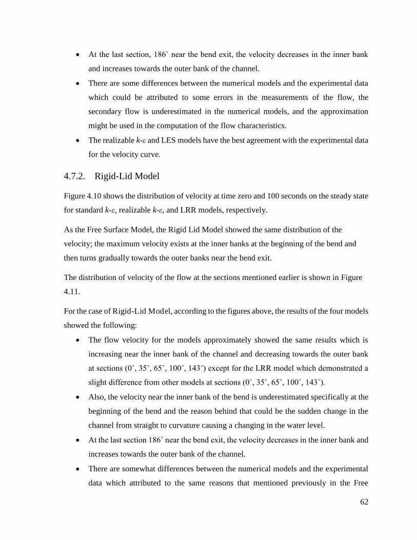
62
At the last section, 186˚ near the bend exit, the velocity decreases in the inner bank
and increases towards the outer bank of the channel.
There are some differences between the numerical models and the experimental data
which could be attributed to some errors in the measurements of the flow, the
secondary flow is underestimated in the numerical models, and the approximation
might be used in the computation of the flow characteristics.
The realizable k-ε and LES models have the best agreement with the experimental data
for the velocity curve.
4.7.2. Rigid-Lid Model
Figure 4.10 shows the distribution of velocity at time zero and 100 seconds on the steady state
for standard k-ε, realizable k-ε, and LRR models, respectively.
As the Free Surface Model, the Rigid Lid Model showed the same distribution of the
velocity; the maximum velocity exists at the inner banks at the beginning of the bend and
then turns gradually towards the outer banks near the bend exit.
The distribution of velocity of the flow at the sections mentioned earlier is shown in Figure
4.11.
For the case of Rigid-Lid Model, according to the figures above, the results of the four models
showed the following:
The flow velocity for the models approximately showed the same results which is
increasing near the inner bank of the channel and decreasing towards the outer bank
at sections (0˚, 35˚, 65˚, 100˚, 143˚) except for the LRR model which demonstrated a
slight difference from other models at sections (0˚, 35˚, 65˚, 100˚, 143˚).
Also, the velocity near the inner bank of the bend is underestimated specifically at the
beginning of the bend and the reason behind that could be the sudden change in the
channel from straight to curvature causing a changing in the water level.
At the last section 186˚ near the bend exit, the velocity decreases in the inner bank and
increases towards the outer bank of the channel.
There are somewhat differences between the numerical models and the experimental
data which attributed to the same reasons that mentioned previously in the Free
63
Surface Model.
The best models that achieved a good agreement in the velocity curve with the
experimental data are the standard k-ε and realizable k-ε models.
a- Velocity at time=0 sec and D=0.058 m. b- Velocity at time=100 sec and D=0.058 m.
Standard k-ε model.
c- Velocity at time=0 sec and D=0.058 m. d- Velocity at time=100 sec and D=0.058 m.
Realizable k-ε model.
e- Velocity at time=0 sec and D=0.058 m. f- Velocity at time=100 sec and D=0.058 m.
LRR model.
Figure 4.10: Rigid Lid Models.
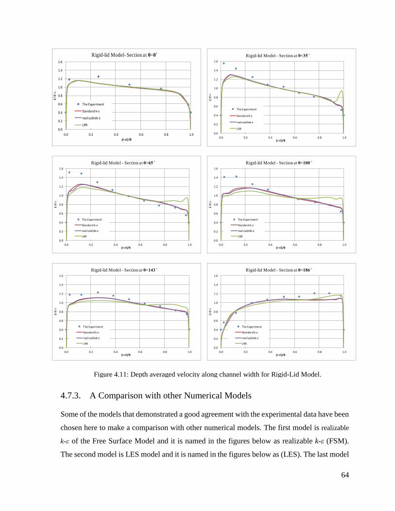
64
4.7.3. A Comparison with other Numerical Models
Some of the models that demonstrated a good agreement with the experimental data have been
chosen here to make a comparison with other numerical models. The first model is realizable
k-ε of the Free Surface Model and it is named in the figures below as realizable k-ε (FSM).
The second model is LES model and it is named in the figures below as (LES). The last model
Figure 4.11: Depth averaged velocity along channel width for Rigid-Lid Model.
0.0
0.2
0.4
0.6
0.8
1.0
1.2
1.4
1.6
0.0 0.2 0.4 0.6 0.8 1.0
U/U
∞
(r-ri)/B
Rigid-lid Model- Section at θ=0˚
The Experiment
Standard k-ε
realizablek-ε
LRR
0.0
0.2
0.4
0.6
0.8
1.0
1.2
1.4
1.6
0.0 0.2 0.4 0.6 0.8 1.0
U/U
∞
(r-ri)/B
Rigid-lid Model - Section at θ=35
The Experiment
Standard k-ε
realizablek-ε
LRR
0.0
0.2
0.4
0.6
0.8
1.0
1.2
1.4
1.6
0.0 0.2 0.4 0.6 0.8 1.0
U/U
∞
(r-ri)/B
Rigid-lid Model - Section at θ=65
The Experiment
Standard k-ε
realizablek-ε
LRR
0.0
0.2
0.4
0.6
0.8
1.0
1.2
1.4
1.6
0.0 0.2 0.4 0.6 0.8 1.0
U/U
∞
(r-ri)/B
Rigid-lid Model - Section at θ=100
The Experiment
Standard k-ε
realizablek-ε
LRR
0.0
0.2
0.4
0.6
0.8
1.0
1.2
1.4
1.6
0.0 0.2 0.4 0.6 0.8 1.0
U/U
∞
(r-ri)/B
Rigid-lid Model - Section at θ=143
The Experiment
Standard k-ε
realizablek-ε
LRR
0.0
0.2
0.4
0.6
0.8
1.0
1.2
1.4
1.6
0.0 0.2 0.4 0.6 0.8 1.0
U/U
∞
(r-ri)/B
Rigid-lid Model - Section at θ=186
The Experiment
Standard k-ε
realizablek-ε
LRR
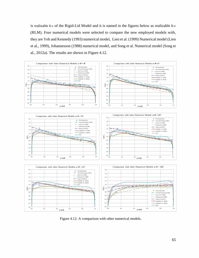
65
is realizable k-ε of the Rigid-Lid Model and it is named in the figures below as realizable k-ε
(RLM). Four numerical models were selected to compare the new employed models with,
they are Yeh and Kennedy (1993) numerical model, Lien et al. (1999) Numerical model (Lien
et al., 1999), Johannesson (1988) numerical model, and Song et al. Numerical model (Song et
al., 2012a). The results are shown in Figure 4.12.
Figure 4.12: A comparison with other numerical models.
0.0
0.2
0.4
0.6
0.8
1.0
1.2
1.4
1.6
1.8
2.0
0.0 0.2 0.4 0.6 0.8 1.0
U/U
∞
(r-ri)/B
Comparison with other Numerical Models at θ = 0˚
The Experiment
Yeh and Kennedy (1993)
Lien et al. (1999)
Johannesson (1988)
Song et al.(2012)
realizable k-ɛ (FSM)
realizable k-ɛ (RLM)
LES
0.0
0.2
0.4
0.6
0.8
1.0
1.2
1.4
1.6
1.8
2.0
0.0 0.2 0.4 0.6 0.8 1.0U
/U∞
(r-ri)/B
Comparison with other Numerical Models at θ=35˚
The Experiment
Yeh and Kennedy (1993)
Lien et al. (1999)
Johannesson (1988)
Song et al.(2012)
realizable k-ɛ (FSM)
realizable k-ɛ (RLM)
LES
0.0
0.2
0.4
0.6
0.8
1.0
1.2
1.4
1.6
1.8
2.0
0.0 0.2 0.4 0.6 0.8 1.0
U/U
∞
(r-ri)/B
Comparison with other Numerical Models at θ = 65˚
The Experiment
Yeh and Kennedy (1993)
Lien et al. (1999)
Johannesson (1988)
Song et al.(2012)
realizable k-ɛ (FSM)
realizable k-ɛ (RLM)
LES
0.0
0.2
0.4
0.6
0.8
1.0
1.2
1.4
1.6
1.8
2.0
0.0 0.2 0.4 0.6 0.8 1.0
U/U
∞
(r-ri)/B
Comparison with other Numerical Models at θ= 100˚
The Experiment
Yeh and Kennedy (1993)
Lien et al. (1999)
Johannesson (1988)
Song et al.(2012)
realizable k-ɛ (FSM)
realizable k-ɛ (RLM)
LES
0.0
0.2
0.4
0.6
0.8
1.0
1.2
1.4
1.6
1.8
2.0
0.0 0.2 0.4 0.6 0.8 1.0
U/U
∞
(r-ri)/B
Comparison with other Numerical Models at θ= 143˚
The Experiment
Yeh and Kennedy (1993)
Lien et al. (1999)
Johannesson (1988)
Song et al.(2012)
realizable k-ɛ (FSM)
realizable k-ɛ (RLM)
LES
0.0
0.2
0.4
0.6
0.8
1.0
1.2
1.4
1.6
1.8
2.0
0.0 0.2 0.4 0.6 0.8 1.0
U/U
∞
(r-ri)/B
Comparison with other Numerical Models at θ = 186˚
The Experiment
Yeh and Kennedy (1993)
Lien et al. (1999)
Johannesson (1988)
Song et al.(2012)
realizable k-ɛ (FSM)
realizable k-ɛ (RLM)
LES
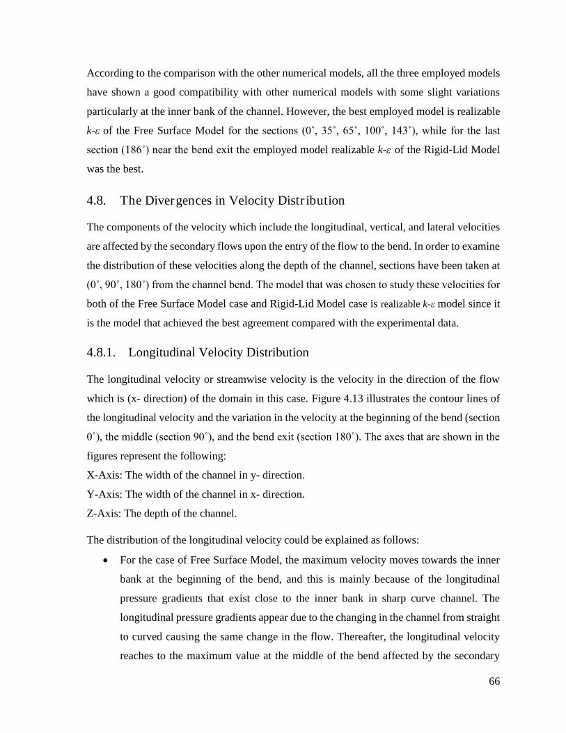
66
According to the comparison with the other numerical models, all the three employed models
have shown a good compatibility with other numerical models with some slight variations
particularly at the inner bank of the channel. However, the best employed model is realizable
k-ε of the Free Surface Model for the sections (0˚, 35˚, 65˚, 100˚, 143˚), while for the last
section (186˚) near the bend exit the employed model realizable k-ε of the Rigid-Lid Model
was the best.
4.8. The Divergences in Velocity Distribution
The components of the velocity which include the longitudinal, vertical, and lateral velocities
are affected by the secondary flows upon the entry of the flow to the bend. In order to examine
the distribution of these velocities along the depth of the channel, sections have been taken at
(0˚, 90˚, 180˚) from the channel bend. The model that was chosen to study these velocities for
both of the Free Surface Model case and Rigid-Lid Model case is realizable k-ε model since it
is the model that achieved the best agreement compared with the experimental data.
4.8.1. Longitudinal Velocity Distribution
The longitudinal velocity or streamwise velocity is the velocity in the direction of the flow
which is (x- direction) of the domain in this case. Figure 4.13 illustrates the contour lines of
the longitudinal velocity and the variation in the velocity at the beginning of the bend (section
0˚), the middle (section 90˚), and the bend exit (section 180˚). The axes that are shown in the
figures represent the following:
X-Axis: The width of the channel in y- direction.
Y-Axis: The width of the channel in x- direction.
Z-Axis: The depth of the channel.
The distribution of the longitudinal velocity could be explained as follows:
For the case of Free Surface Model, the maximum velocity moves towards the inner
bank at the beginning of the bend, and this is mainly because of the longitudinal
pressure gradients that exist close to the inner bank in sharp curve channel. The
longitudinal pressure gradients appear due to the changing in the channel from straight
to curved causing the same change in the flow. Thereafter, the longitudinal velocity
reaches to the maximum value at the middle of the bend affected by the secondary
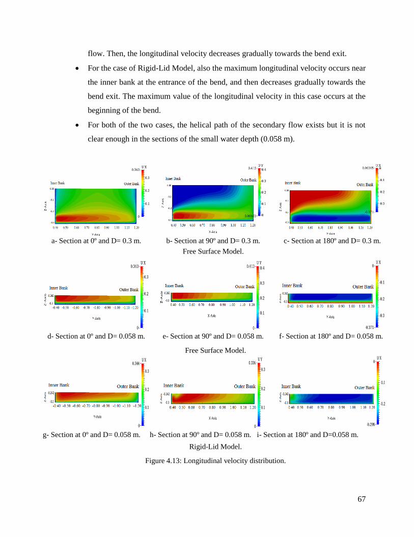
67
flow. Then, the longitudinal velocity decreases gradually towards the bend exit.
For the case of Rigid-Lid Model, also the maximum longitudinal velocity occurs near
the inner bank at the entrance of the bend, and then decreases gradually towards the
bend exit. The maximum value of the longitudinal velocity in this case occurs at the
beginning of the bend.
For both of the two cases, the helical path of the secondary flow exists but it is not
clear enough in the sections of the small water depth (0.058 m).
a- Section at 0º and D= 0.3 m. b- Section at 90º and D= 0.3 m. c- Section at 180º and D= 0.3 m.
Free Surface Model.
d- Section at 0º and D= 0.058 m. e- Section at 90º and D= 0.058 m. f- Section at 180º and D= 0.058 m.
Free Surface Model.
g- Section at 0º and D= 0.058 m. h- Section at 90º and D= 0.058 m. i- Section at 180º and D=0.058 m.
Rigid-Lid Model.
Figure 4.13: Longitudinal velocity distribution.
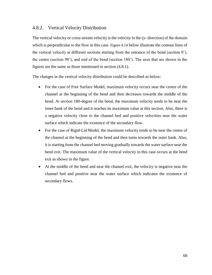
68
4.8.2. Vertical Velocity Distribution
The vertical velocity or cross-stream velocity is the velocity in the (y- direction) of the domain
which is perpendicular to the flow in this case. Figure 4.14 below illustrate the contour lines of
the vertical velocity at different sections starting from the entrance of the bend (section 0˚),
the centre (section 90˚), and end of the bend (section 180˚). The axes that are shown in the
figures are the same as those mentioned in section (4.8.1).
The changes in the vertical velocity distribution could be described as below:
For the case of Free Surface Model, maximum velocity occurs near the centre of the
channel at the beginning of the bend and then decreases towards the middle of the
bend. At section 180-degree of the bend, the maximum velocity tends to be near the
inner bank of the bend and it reaches its maximum value at this section. Also, there is
a negative velocity close to the channel bed and positive velocities near the water
surface which indicate the existence of the secondary flow.
For the case of Rigid-Lid Model, the maximum velocity tends to be near the centre of
the channel at the beginning of the bend and then turns towards the outer bank. Also,
it is starting from the channel bed moving gradually towards the water surface near the
bend exit. The maximum value of the vertical velocity in this case occurs at the bend
exit as shown in the figure.
At the middle of the bend and near the channel exit, the velocity is negative near the
channel bed and positive near the water surface which indicates the existence of
secondary flows.
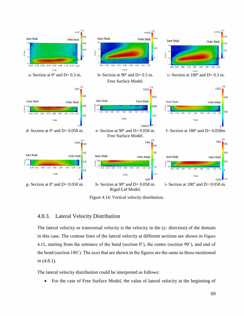
69
4.8.3. Lateral Velocity Distribution
The lateral velocity or transversal velocity is the velocity in the (z- direction) of the domain
in this case. The contour lines of the lateral velocity at different sections are shown in Figure
4.15, starting from the entrance of the bend (section 0˚), the centre (section 90˚), and end of
the bend (section 180˚). The axes that are shown in the figures are the same as those mentioned
in (4.8.1).
The lateral velocity distribution could be interpreted as follows:
For the case of Free Surface Model, the value of lateral velocity at the beginning of
a- Section at 0º and D= 0.3 m. b- Section at 90º and D= 0.3 m. c- Section at 180º and D= 0.3 m.
Free Surface Model.
d- Section at 0º and D= 0.058 m. e- Section at 90º and D= 0.058 m. f- Section at 180º and D= 0.058m.
Free Surface Model.
g- Section at 0º and D= 0.058 m. h- Section at 90º and D= 0.058 m. i- Section at 180º and D= 0.058 m.
Rigid-Lid Model.
Figure 4.14: Vertical velocity distribution.
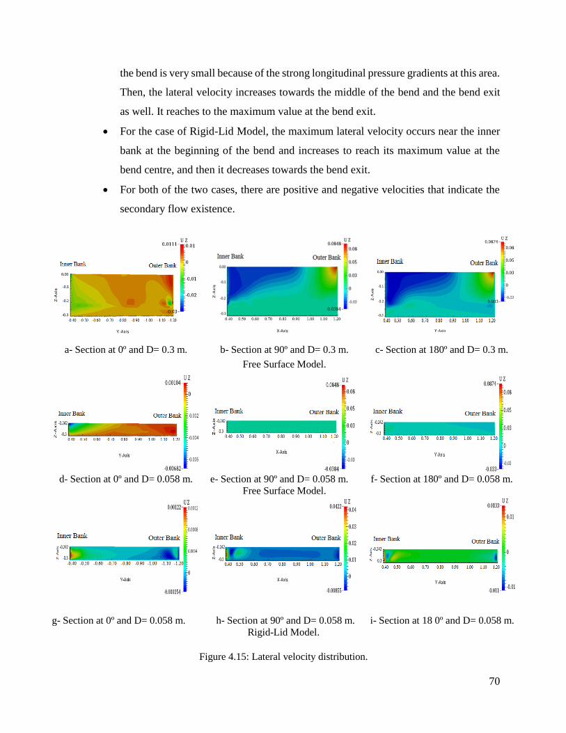
70
the bend is very small because of the strong longitudinal pressure gradients at this area.
Then, the lateral velocity increases towards the middle of the bend and the bend exit
as well. It reaches to the maximum value at the bend exit.
For the case of Rigid-Lid Model, the maximum lateral velocity occurs near the inner
bank at the beginning of the bend and increases to reach its maximum value at the
bend centre, and then it decreases towards the bend exit.
For both of the two cases, there are positive and negative velocities that indicate the
secondary flow existence.
a- Section at 0º and D= 0.3 m. b- Section at 90º and D= 0.3 m. c- Section at 180º and D= 0.3 m.
Free Surface Model.
d- Section at 0º and D= 0.058 m. e- Section at 90º and D= 0.058 m. f- Section at 180º and D= 0.058 m.
Free Surface Model.
g- Section at 0º and D= 0.058 m. h- Section at 90º and D= 0.058 m. i- Section at 18 0º and D= 0.058 m.
Rigid-Lid Model.
Figure 4.15: Lateral velocity distribution.
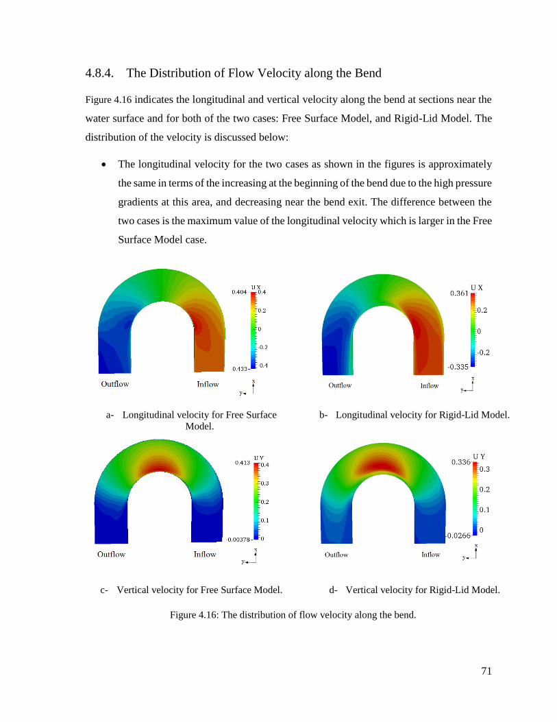
71
4.8.4. The Distribution of Flow Velocity along the Bend
Figure 4.16 indicates the longitudinal and vertical velocity along the bend at sections near the
water surface and for both of the two cases: Free Surface Model, and Rigid-Lid Model. The
distribution of the velocity is discussed below:
The longitudinal velocity for the two cases as shown in the figures is approximately
the same in terms of the increasing at the beginning of the bend due to the high pressure
gradients at this area, and decreasing near the bend exit. The difference between the
two cases is the maximum value of the longitudinal velocity which is larger in the Free
Surface Model case.
a- Longitudinal velocity for Free Surface
Model.
b- Longitudinal velocity for Rigid-Lid Model.
c- Vertical velocity for Free Surface Model. d- Vertical velocity for Rigid-Lid Model.
Figure 4.16: The distribution of flow velocity along the bend.
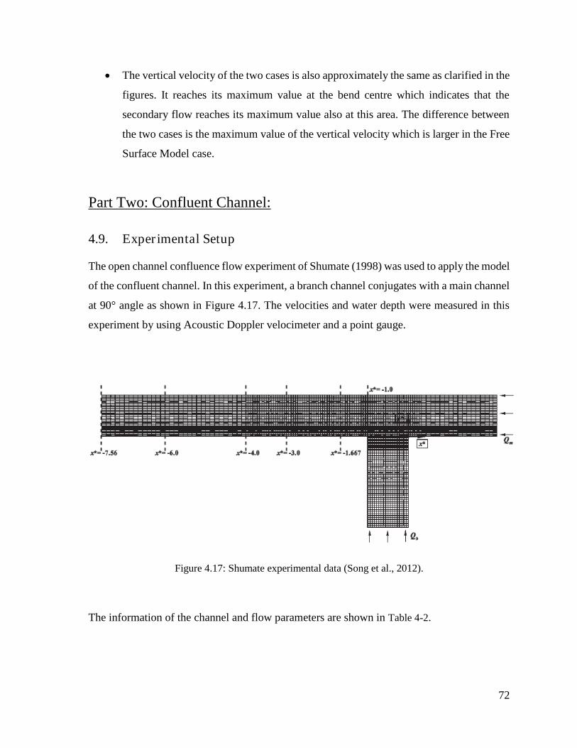
72
The vertical velocity of the two cases is also approximately the same as clarified in the
figures. It reaches its maximum value at the bend centre which indicates that the
secondary flow reaches its maximum value also at this area. The difference between
the two cases is the maximum value of the vertical velocity which is larger in the Free
Surface Model case.
Part Two: Confluent Channel:
4.9. Experimental Setup
The open channel confluence flow experiment of Shumate (1998) was used to apply the model
of the confluent channel. In this experiment, a branch channel conjugates with a main channel
at 90° angle as shown in Figure 4.17. The velocities and water depth were measured in this
experiment by using Acoustic Doppler velocimeter and a point gauge.
Figure 4.17: Shumate experimental data (Song et al., 2012).
The information of the channel and flow parameters are shown in Table 4-2.
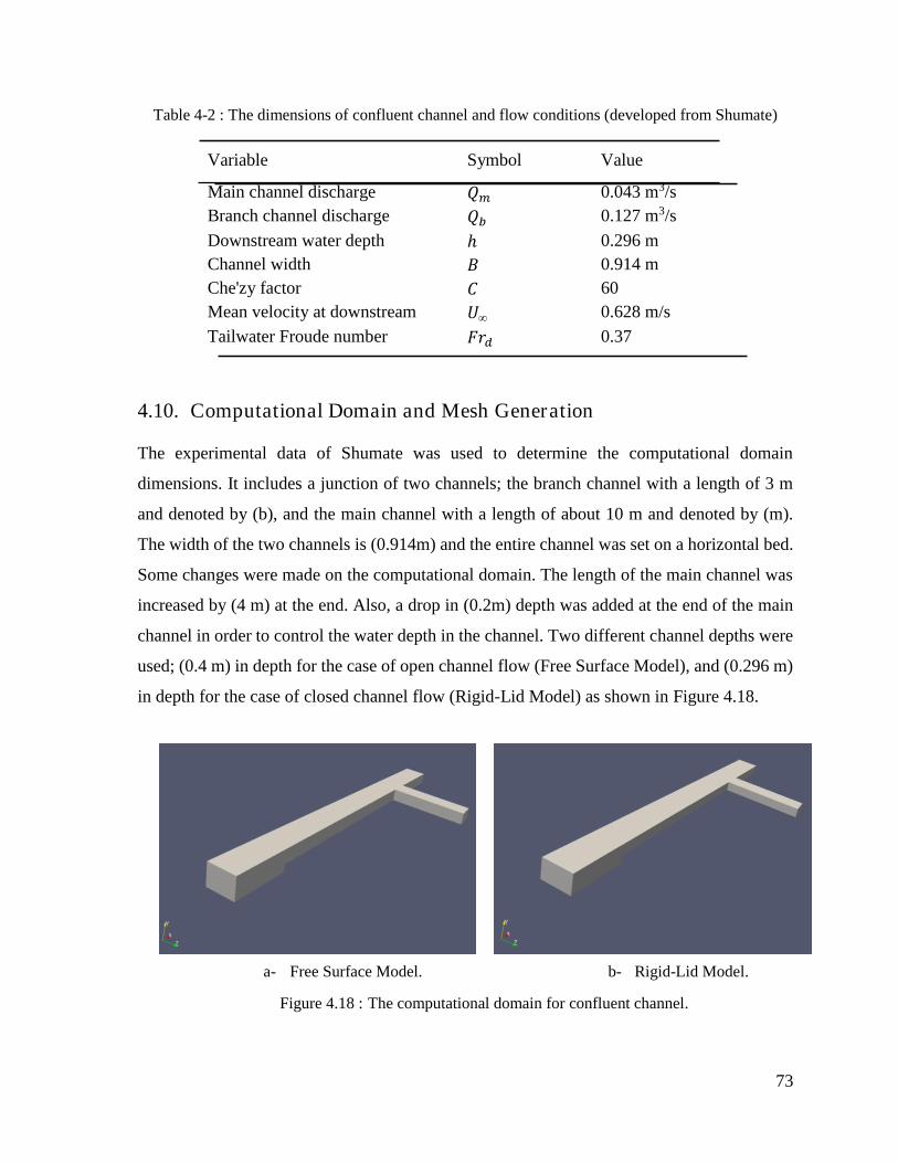
73
Table 4-2 : The dimensions of confluent channel and flow conditions (developed from Shumate)
Variable Symbol Value
Main channel discharge 𝑄𝑚 0.043 m3/s
Branch channel discharge 𝑄𝑏 0.127 m3/s
Downstream water depth ℎ 0.296 m
Channel width 𝐵 0.914 m
Che'zy factor 𝐶 60
Mean velocity at downstream 𝑈∞ 0.628 m/s
Tailwater Froude number 𝐹𝑟𝑑 0.37
4.10. Computational Domain and Mesh Generation
The experimental data of Shumate was used to determine the computational domain
dimensions. It includes a junction of two channels; the branch channel with a length of 3 m
and denoted by (b), and the main channel with a length of about 10 m and denoted by (m).
The width of the two channels is (0.914m) and the entire channel was set on a horizontal bed.
Some changes were made on the computational domain. The length of the main channel was
increased by (4 m) at the end. Also, a drop in (0.2m) depth was added at the end of the main
channel in order to control the water depth in the channel. Two different channel depths were
used; (0.4 m) in depth for the case of open channel flow (Free Surface Model), and (0.296 m)
in depth for the case of closed channel flow (Rigid-Lid Model) as shown in Figure 4.18.
a- Free Surface Model. b- Rigid-Lid Model.
Figure 4.18 : The computational domain for confluent channel.
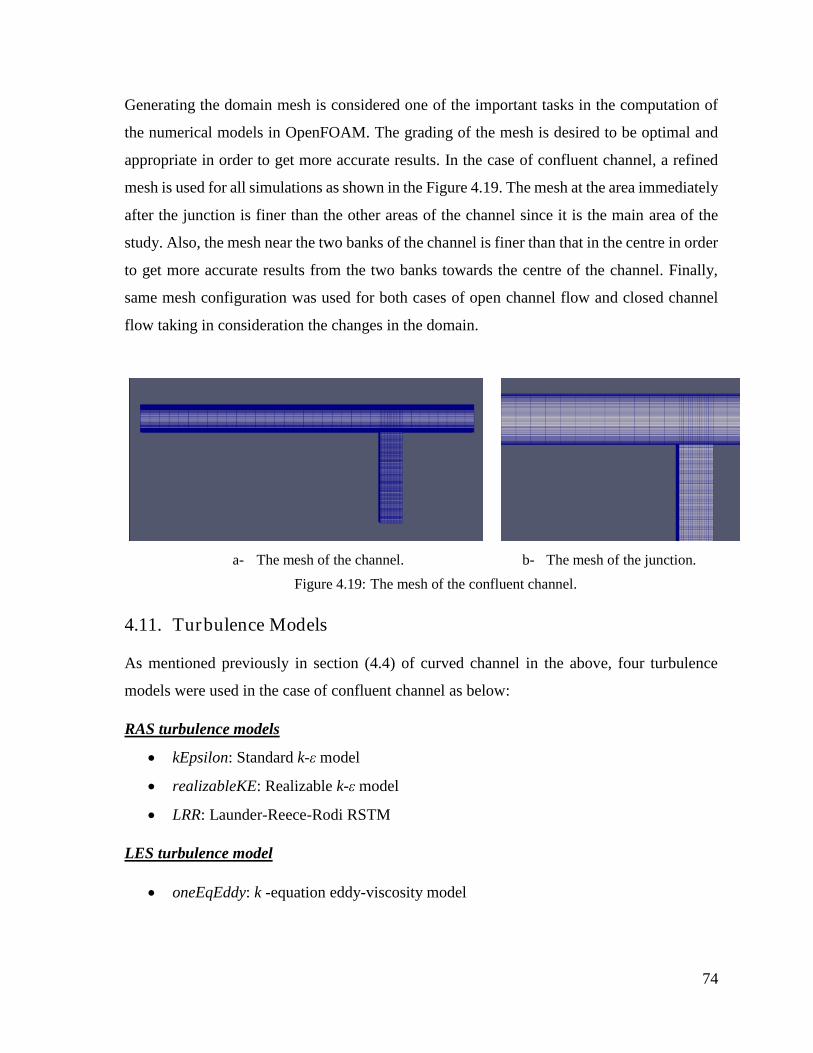
74
Generating the domain mesh is considered one of the important tasks in the computation of
the numerical models in OpenFOAM. The grading of the mesh is desired to be optimal and
appropriate in order to get more accurate results. In the case of confluent channel, a refined
mesh is used for all simulations as shown in the Figure 4.19. The mesh at the area immediately
after the junction is finer than the other areas of the channel since it is the main area of the
study. Also, the mesh near the two banks of the channel is finer than that in the centre in order
to get more accurate results from the two banks towards the centre of the channel. Finally,
same mesh configuration was used for both cases of open channel flow and closed channel
flow taking in consideration the changes in the domain.
4.11. Turbulence Models
As mentioned previously in section (4.4) of curved channel in the above, four turbulence
models were used in the case of confluent channel as below:
RAS turbulence models
kEpsilon: Standard k-ε model
realizableKE: Realizable k-ε model
LRR: Launder-Reece-Rodi RSTM
LES turbulence model
oneEqEddy: k -equation eddy-viscosity model
a- The mesh of the channel. b- The mesh of the junction.
Figure 4.19: The mesh of the confluent channel.
75
4.12. The Numerical Simulations
As mentioned in Section (4.5) of curved channel, OpenFOAM was used in the simulation of
this study.
4.13. Initial and Boundary Conditions
The initial and boundary conditions used in the confluent channel are the same as those
mentioned in Section (4.6), which was used in the curved channel.
4.14. Results and Discussions
Due to the complexity of flow features in river confluences and its importance in river
engineering, several studies were reviewed to better understand these features. In this study,
the velocity parameters were used to evaluate the models because of its capability on
visualizing the flow characteristics. The results of the velocities across dimensional channel
width that obtained from the different models were compared with Shumate experimental data
(1998). Also, the components of the velocity in three dimensions were studied, and reasons
behind the difference in each velocity were examined. Finally, the best model for each case
was selected after evaluating the results of each model.
4.14.1. Free Surface Model
In this case of open channel flow, the flow features in the confluences were studied for the
water flow separately without the effects of the air. To achieve that, a horizontal section was
taken on depth of (0.104 m) from the top of the channel. Consequently, the total depth of the
channel is (𝐷𝑡 = 0.4 m) and the depth of water after the steady state is (𝐷𝑓 = 0.296m), which
are the same depths in Shumate experiment.
For all models (standard k-ε, LRR, realizable k-ε, and LES models), the depth of water at time
zero was (0.096 m), and approximately (0.296 m) at the steady state as shown in figures 4-20
to 4-23. Noting that the calculated velocity considering the air and depth of water is shown in
parts (c) and (d), while parts (e) and (f) consider the depth of water only. The latter case was
adopted in this research.
The velocity distribution of the four models could be discussed as following:
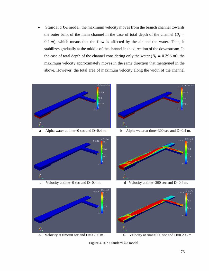
76
Standard k-ε model: the maximum velocity moves from the branch channel towards
the outer bank of the main channel in the case of total depth of the channel (𝐷𝑡 =
0.4 𝑚), which means that the flow is affected by the air and the water. Then, it
stabilizes gradually at the middle of the channel in the direction of the downstream. In
the case of total depth of the channel considering only the water (𝐷𝑡 = 0.296 𝑚), the
maximum velocity approximately moves in the same direction that mentioned in the
above. However, the total area of maximum velocity along the width of the channel
a- Alpha water at time=0 sec and D=0.4 m. b- Alpha water at time=300 sec and D=0.4 m.
c- Velocity at time=0 sec and D=0.4 m. d- Velocity at time=300 sec and D=0.4 m.
e- Velocity at time=0 sec and D=0.296 m. f- Velocity at time=300 sec and D=0.296 m.
Figure 4.20 : Standard k-ε model.
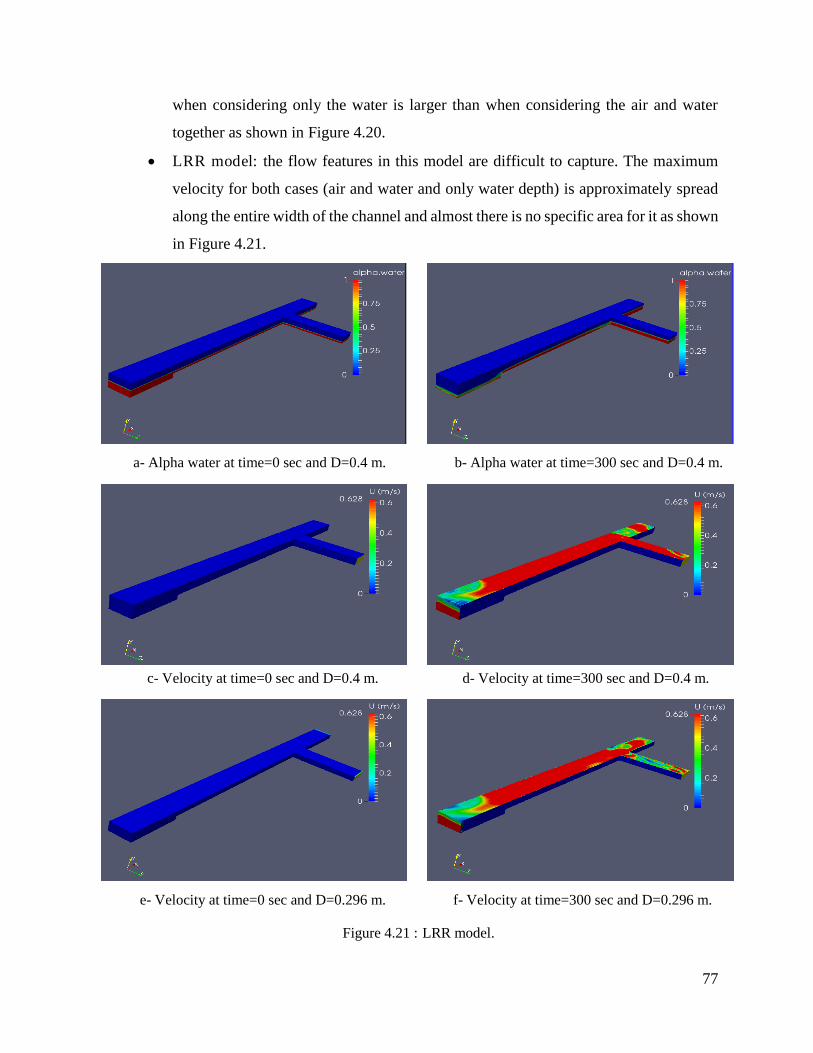
77
when considering only the water is larger than when considering the air and water
together as shown in Figure 4.20.
LRR model: the flow features in this model are difficult to capture. The maximum
velocity for both cases (air and water and only water depth) is approximately spread
along the entire width of the channel and almost there is no specific area for it as shown
in Figure 4.21.
a- Alpha water at time=0 sec and D=0.4 m. b- Alpha water at time=300 sec and D=0.4 m.
c- Velocity at time=0 sec and D=0.4 m. d- Velocity at time=300 sec and D=0.4 m.
e- Velocity at time=0 sec and D=0.296 m. f- Velocity at time=300 sec and D=0.296 m.
Figure 4.21 : LRR model.
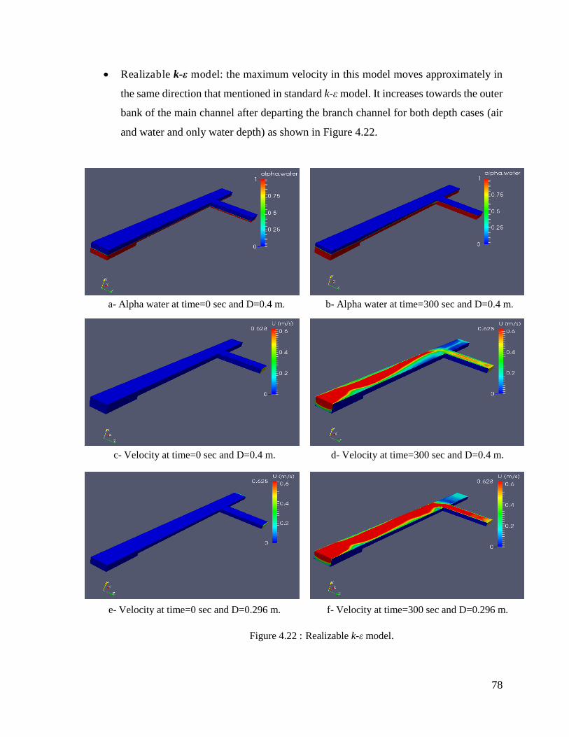
78
Realizable k-ε model: the maximum velocity in this model moves approximately in
the same direction that mentioned in standard k-ε model. It increases towards the outer
bank of the main channel after departing the branch channel for both depth cases (air
and water and only water depth) as shown in Figure 4.22.
a- Alpha water at time=0 sec and D=0.4 m. b- Alpha water at time=300 sec and D=0.4 m.
c- Velocity at time=0 sec and D=0.4 m. d- Velocity at time=300 sec and D=0.4 m.
e- Velocity at time=0 sec and D=0.296 m. f- Velocity at time=300 sec and D=0.296 m.
Figure 4.22 : Realizable k-ε model.
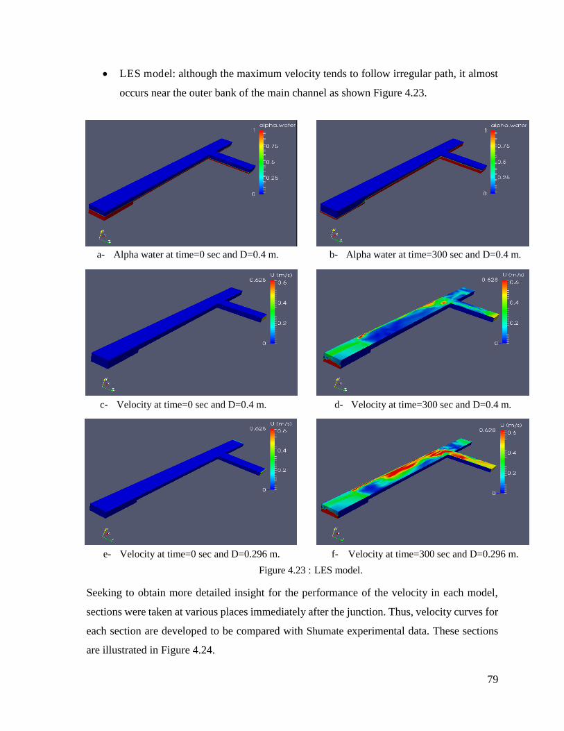
79
LES model: although the maximum velocity tends to follow irregular path, it almost
occurs near the outer bank of the main channel as shown Figure 4.23.
Seeking to obtain more detailed insight for the performance of the velocity in each model,
sections were taken at various places immediately after the junction. Thus, velocity curves for
each section are developed to be compared with Shumate experimental data. These sections
are illustrated in Figure 4.24.
a- Alpha water at time=0 sec and D=0.4 m. b- Alpha water at time=300 sec and D=0.4 m.
c- Velocity at time=0 sec and D=0.4 m. d- Velocity at time=300 sec and D=0.4 m.
e- Velocity at time=0 sec and D=0.296 m. f- Velocity at time=300 sec and D=0.296 m.
Figure 4.23 : LES model.
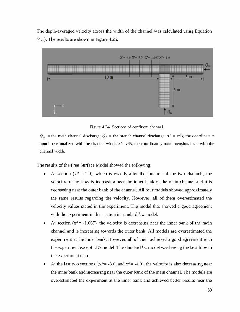
80
The depth-averaged velocity across the width of the channel was calculated using Equation
(4.1). The results are shown in Figure 4.25.
The results of the Free Surface Model showed the following:
At section (x*= -1.0), which is exactly after the junction of the two channels, the
velocity of the flow is increasing near the inner bank of the main channel and it is
decreasing near the outer bank of the channel. All four models showed approximately
the same results regarding the velocity. However, all of them overestimated the
velocity values stated in the experiment. The model that showed a good agreement
with the experiment in this section is standard k-ε model.
At section (x*= -1.667), the velocity is decreasing near the inner bank of the main
channel and is increasing towards the outer bank. All models are overestimated the
experiment at the inner bank. However, all of them achieved a good agreement with
the experiment except LES model. The standard k-ε model was having the best fit with
the experiment data.
At the last two sections, (x*= -3.0, and x*= -4.0), the velocity is also decreasing near
the inner bank and increasing near the outer bank of the main channel. The models are
overestimated the experiment at the inner bank and achieved better results near the
Figure 4.24: Sections of confluent channel.
𝑸𝒎 = the main channel discharge; 𝑸𝒃 = the branch channel discharge; 𝒙∗ = x/B, the coordinate x
nondimensionalized with the channel width; 𝒛∗= z/B, the coordinate y nondimensionalized with the
channel width.
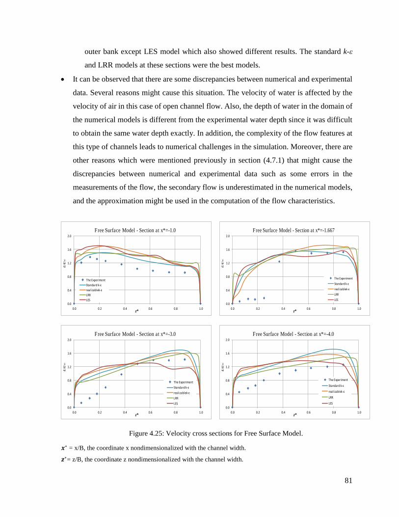
81
outer bank except LES model which also showed different results. The standard k-ε
and LRR models at these sections were the best models.
It can be observed that there are some discrepancies between numerical and experimental
data. Several reasons might cause this situation. The velocity of water is affected by the
velocity of air in this case of open channel flow. Also, the depth of water in the domain of
the numerical models is different from the experimental water depth since it was difficult
to obtain the same water depth exactly. In addition, the complexity of the flow features at
this type of channels leads to numerical challenges in the simulation. Moreover, there are
other reasons which were mentioned previously in section (4.7.1) that might cause the
discrepancies between numerical and experimental data such as some errors in the
measurements of the flow, the secondary flow is underestimated in the numerical models,
and the approximation might be used in the computation of the flow characteristics.
Figure 4.25: Velocity cross sections for Free Surface Model.
𝒙∗ = x/B, the coordinate x nondimensionalized with the channel width.
𝒛∗= z/B, the coordinate z nondimensionalized with the channel width.
0.0
0.4
0.8
1.2
1.6
2.0
0.0 0.2 0.4 0.6 0.8 1.0
U/U
∞
z*
Free Surface Model - Section at x*=-1.0
The Experiment
Standard k-ε
realizablek-ε
LRR
LES 0.0
0.4
0.8
1.2
1.6
2.0
0.0 0.2 0.4 0.6 0.8 1.0
U/U
∞
z*
Free Surface Model - Section at x*=-1.667
The Experiment
Standard k-ε
realizablek-ε
LRR
LES
0.0
0.4
0.8
1.2
1.6
2.0
0.0 0.2 0.4 0.6 0.8 1.0
U/U
∞
z*
Free Surface Model - Section at x*=-3.0
The Experiment
Standard k-ε
realizablek-ε
LRR
LES 0.0
0.4
0.8
1.2
1.6
2.0
0.0 0.2 0.4 0.6 0.8 1.0
U/U
∞
z*
Free Surface Model - Section at x*=-4.0
The Experiment
Standard k-ε
realizablek-ε
LRR
LES
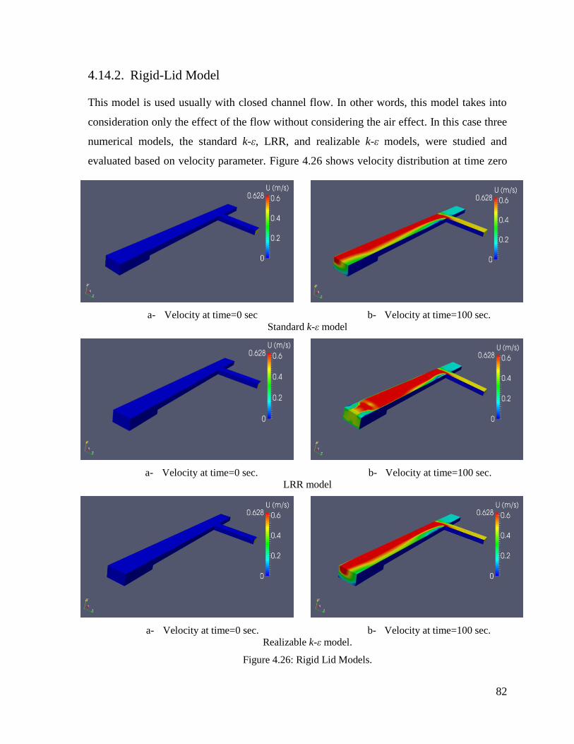
82
4.14.2. Rigid-Lid Model
This model is used usually with closed channel flow. In other words, this model takes into
consideration only the effect of the flow without considering the air effect. In this case three
numerical models, the standard k-ε, LRR, and realizable k-ε models, were studied and
evaluated based on velocity parameter. Figure 4.26 shows velocity distribution at time zero
a- Velocity at time=0 sec b- Velocity at time=100 sec.
Standard k-ε model
a- Velocity at time=0 sec. b- Velocity at time=100 sec.
LRR model
a- Velocity at time=0 sec. b- Velocity at time=100 sec.
Realizable k-ε model.
Figure 4.26: Rigid Lid Models.
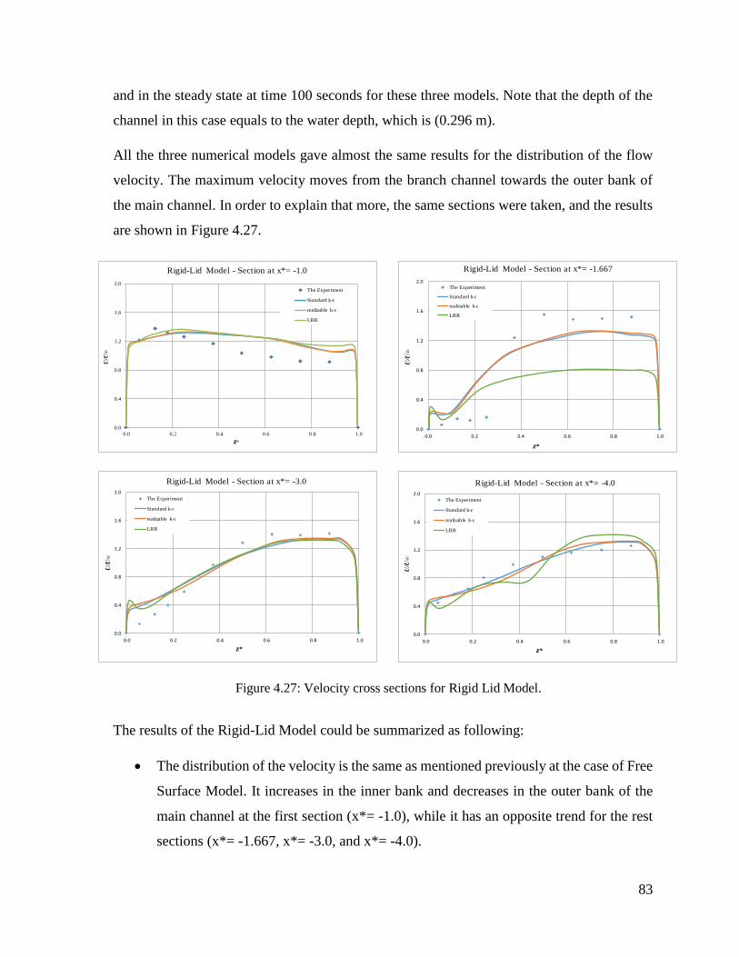
83
and in the steady state at time 100 seconds for these three models. Note that the depth of the
channel in this case equals to the water depth, which is (0.296 m).
All the three numerical models gave almost the same results for the distribution of the flow
velocity. The maximum velocity moves from the branch channel towards the outer bank of
the main channel. In order to explain that more, the same sections were taken, and the results
are shown in Figure 4.27.
The results of the Rigid-Lid Model could be summarized as following:
The distribution of the velocity is the same as mentioned previously at the case of Free
Surface Model. It increases in the inner bank and decreases in the outer bank of the
main channel at the first section (x*= -1.0), while it has an opposite trend for the rest
sections (x*= -1.667, x*= -3.0, and x*= -4.0).
Figure 4.27: Velocity cross sections for Rigid Lid Model.
0.0
0.4
0.8
1.2
1.6
2.0
0.0 0.2 0.4 0.6 0.8 1.0
U/U
∞
z*
Rigid-Lid Model - Section at x*= -1.0
The Experiment
Standard k-ɛ
realizable k-ɛ
LRR
0.0
0.4
0.8
1.2
1.6
2.0
0.0 0.2 0.4 0.6 0.8 1.0
U/U
∞
z*
Rigid-Lid Model - Section at x*= -1.667
The Experiment
Standard k-ɛ
realizable k-ɛ
LRR
0.0
0.4
0.8
1.2
1.6
2.0
0.0 0.2 0.4 0.6 0.8 1.0
U/U
∞
z*
Rigid-Lid Model - Section at x*= -3.0
The Experiment
Standard k-ɛ
realizable k-ɛ
LRR
0.0
0.4
0.8
1.2
1.6
2.0
0.0 0.2 0.4 0.6 0.8 1.0
U/U
∞
z*
Rigid-Lid Model - Section at x*= -4.0
The Experiment
Standard k-ɛ
realizable k-ɛ
LRR
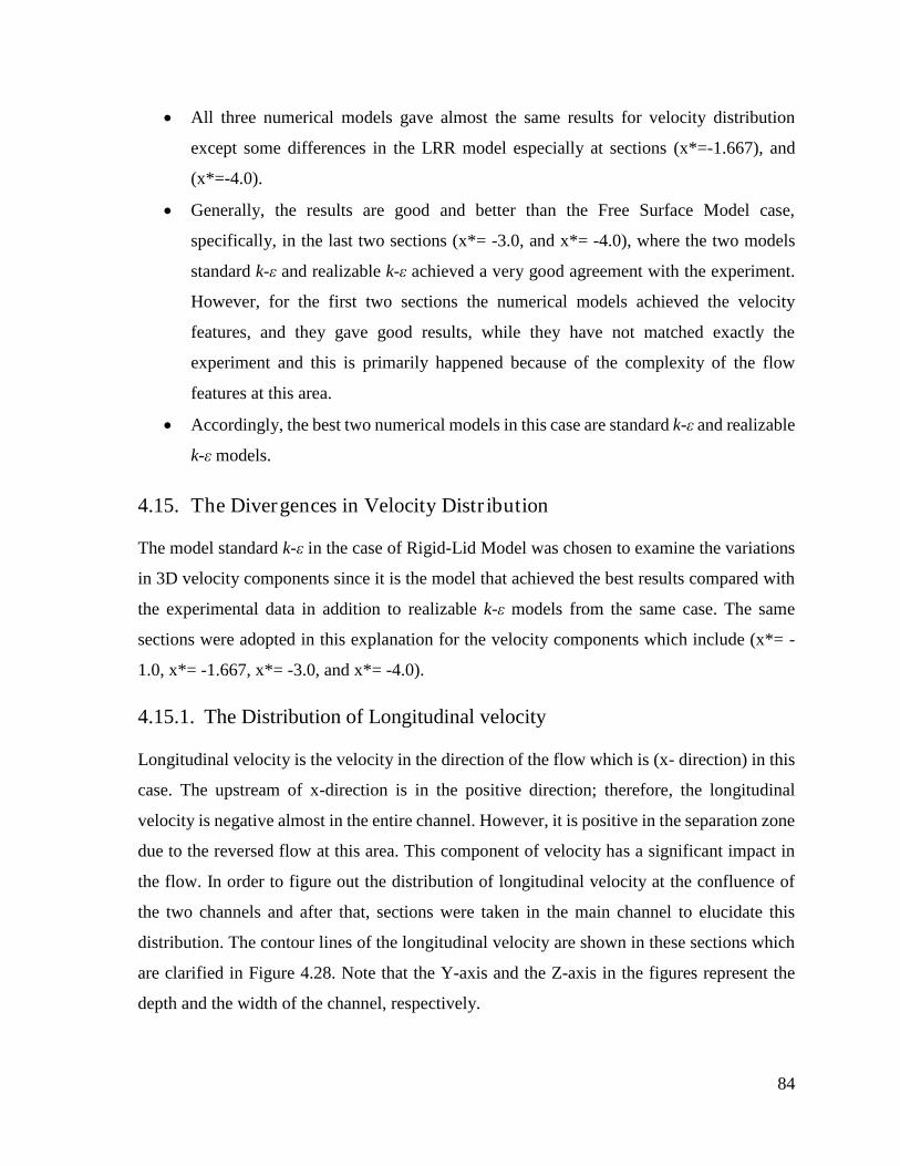
84
All three numerical models gave almost the same results for velocity distribution
except some differences in the LRR model especially at sections (x*=-1.667), and
(x*=-4.0).
Generally, the results are good and better than the Free Surface Model case,
specifically, in the last two sections (x*= -3.0, and x*= -4.0), where the two models
standard k-ε and realizable k-ε achieved a very good agreement with the experiment.
However, for the first two sections the numerical models achieved the velocity
features, and they gave good results, while they have not matched exactly the
experiment and this is primarily happened because of the complexity of the flow
features at this area.
Accordingly, the best two numerical models in this case are standard k-ε and realizable
k-ε models.
4.15. The Divergences in Velocity Distribution
The model standard k-ε in the case of Rigid-Lid Model was chosen to examine the variations
in 3D velocity components since it is the model that achieved the best results compared with
the experimental data in addition to realizable k-ε models from the same case. The same
sections were adopted in this explanation for the velocity components which include (x*= -
1.0, x*= -1.667, x*= -3.0, and x*= -4.0).
4.15.1. The Distribution of Longitudinal velocity
Longitudinal velocity is the velocity in the direction of the flow which is (x- direction) in this
case. The upstream of x-direction is in the positive direction; therefore, the longitudinal
velocity is negative almost in the entire channel. However, it is positive in the separation zone
due to the reversed flow at this area. This component of velocity has a significant impact in
the flow. In order to figure out the distribution of longitudinal velocity at the confluence of
the two channels and after that, sections were taken in the main channel to elucidate this
distribution. The contour lines of the longitudinal velocity are shown in these sections which
are clarified in Figure 4.28. Note that the Y-axis and the Z-axis in the figures represent the
depth and the width of the channel, respectively.
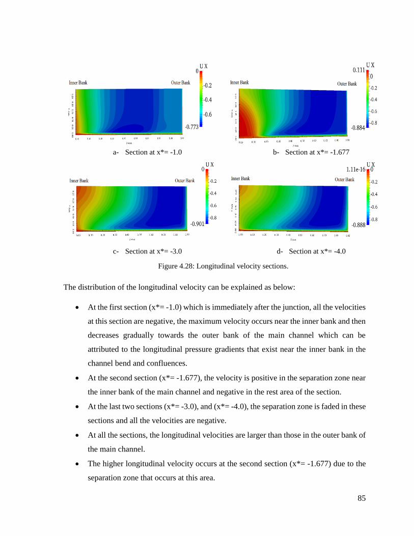
85
The distribution of the longitudinal velocity can be explained as below:
At the first section (x*= -1.0) which is immediately after the junction, all the velocities
at this section are negative, the maximum velocity occurs near the inner bank and then
decreases gradually towards the outer bank of the main channel which can be
attributed to the longitudinal pressure gradients that exist near the inner bank in the
channel bend and confluences.
At the second section (x*= -1.677), the velocity is positive in the separation zone near
the inner bank of the main channel and negative in the rest area of the section.
At the last two sections (x*= -3.0), and (x*= -4.0), the separation zone is faded in these
sections and all the velocities are negative.
At all the sections, the longitudinal velocities are larger than those in the outer bank of
the main channel.
The higher longitudinal velocity occurs at the second section (x*= -1.677) due to the
separation zone that occurs at this area.
a- Section at x*= -1.0 b- Section at x*= -1.677
c- Section at x*= -3.0 d- Section at x*= -4.0
Figure 4.28: Longitudinal velocity sections.
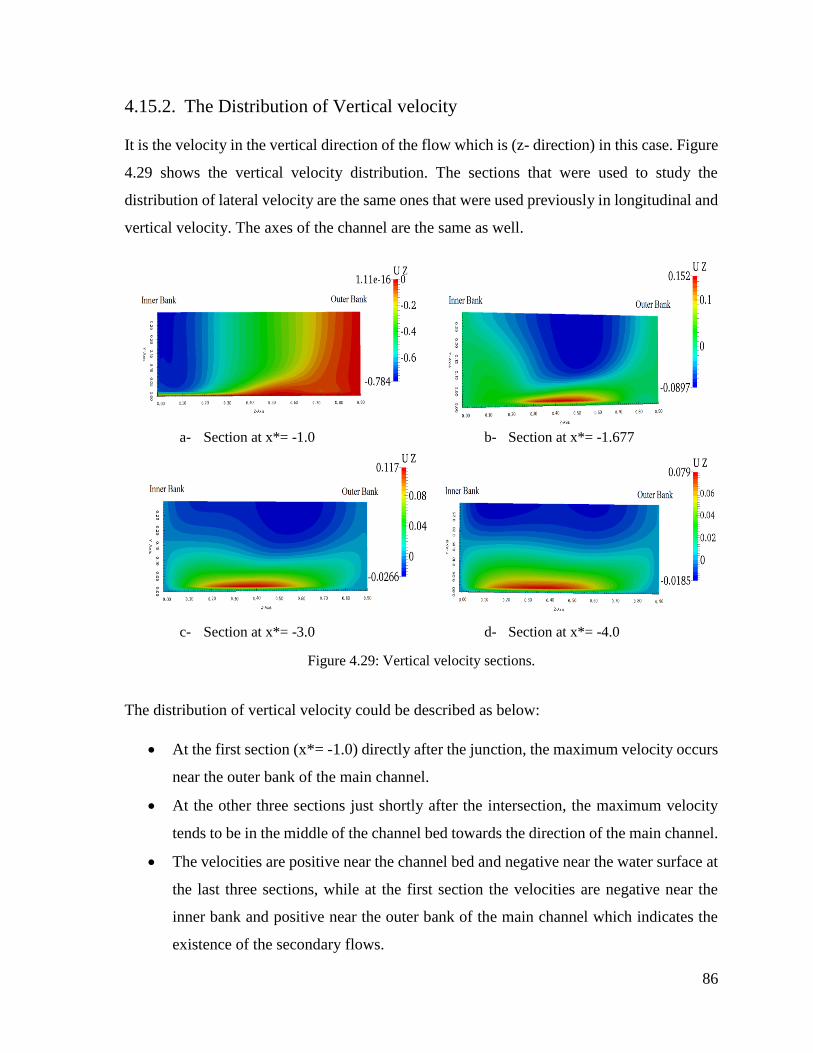
86
4.15.2. The Distribution of Vertical velocity
It is the velocity in the vertical direction of the flow which is (z- direction) in this case. Figure
4.29 shows the vertical velocity distribution. The sections that were used to study the
distribution of lateral velocity are the same ones that were used previously in longitudinal and
vertical velocity. The axes of the channel are the same as well.
a- Section at x*= -1.0 b- Section at x*= -1.677
c- Section at x*= -3.0 d- Section at x*= -4.0
Figure 4.29: Vertical velocity sections.
The distribution of vertical velocity could be described as below:
At the first section (x*= -1.0) directly after the junction, the maximum velocity occurs
near the outer bank of the main channel.
At the other three sections just shortly after the intersection, the maximum velocity
tends to be in the middle of the channel bed towards the direction of the main channel.
The velocities are positive near the channel bed and negative near the water surface at
the last three sections, while at the first section the velocities are negative near the
inner bank and positive near the outer bank of the main channel which indicates the
existence of the secondary flows.
87
The vertical velocity reaches its maximum at the second section at (x*= -1.667).
4.15.3. The Distribution of Lateral velocity
It is the velocity in the (y- direction) of the domain in this case. The distribution of the lateral
velocity has been studied in the light of the same sections that mentioned previously as shown
in Figure 4.30. Also, the two axes have been mentioned in above.
a- Section at x*= -1.0 b- Section at x*= -1.677
c- Section at x*= -3.0 d- Section at x*= -4.0
Figure 4.30: Lateral velocity sections.
The distribution of the vertical velocity could be summarized as following:
At the first section (x*= -1.0) which is immediately after the junction, the recirculation
zone or separation zone appears near the inner bank of the main channel. Also, there
are two secondary flows at this section; the first one is the secondary flow of the branch
channel which occurs near the inner bank of the main channel, and the second is the
secondary flow of the main channel which occurs near the outer bank of the main
channel.
At the second section (x*= -1.677), the separation zone started to disappear.
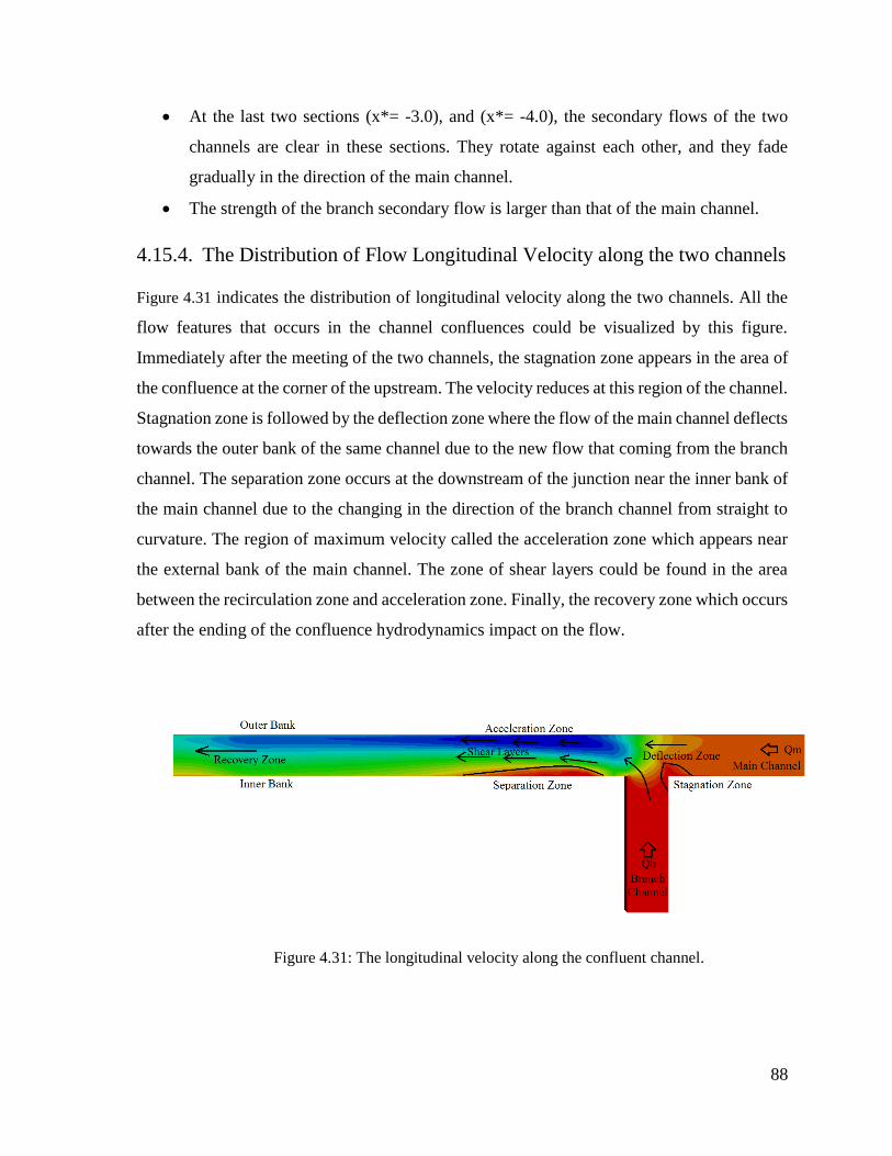
88
At the last two sections (x*= -3.0), and (x*= -4.0), the secondary flows of the two
channels are clear in these sections. They rotate against each other, and they fade
gradually in the direction of the main channel.
The strength of the branch secondary flow is larger than that of the main channel.
4.15.4. The Distribution of Flow Longitudinal Velocity along the two channels
Figure 4.31 indicates the distribution of longitudinal velocity along the two channels. All the
flow features that occurs in the channel confluences could be visualized by this figure.
Immediately after the meeting of the two channels, the stagnation zone appears in the area of
the confluence at the corner of the upstream. The velocity reduces at this region of the channel.
Stagnation zone is followed by the deflection zone where the flow of the main channel deflects
towards the outer bank of the same channel due to the new flow that coming from the branch
channel. The separation zone occurs at the downstream of the junction near the inner bank of
the main channel due to the changing in the direction of the branch channel from straight to
curvature. The region of maximum velocity called the acceleration zone which appears near
the external bank of the main channel. The zone of shear layers could be found in the area
between the recirculation zone and acceleration zone. Finally, the recovery zone which occurs
after the ending of the confluence hydrodynamics impact on the flow.
Figure 4.31: The longitudinal velocity along the confluent channel.
89
CHAPTER FIVE
5. CONCLUSIONS AND SUGGESTIONS FOR FUTURE WORK
5.1. Conclusions
Studying the characteristics of the flow in river bends and confluences could be considered
one of the important tasks in river engineering due to the significant existence of curvature
and confluences in rivers and their great impact on river engineering problems. However,
examining the dynamic of the flow in river bends and confluences is a hard task because of
the complexity of flow features at this area, which makes it difficult to be captured and
determined. Secondary flow is one of the flow characteristics in curved and confluent rivers.
In this study, secondary currents were studied by employing a 3D OpenFOAM numerical
model. Basically, OpenFOAM depends on the finite volume method (FVM), which includes
a lot of numerical schemes that are implemented both for time and space integration. Two sets
of experimental data were used to validate the proposed model. Two solvers were used; the
InterFoam solver which is used in open channel flow (Free Surface Model), and the PisoFoam
solver which is used in closed channel flow (Rigid-Lid Model). Various turbulence models
(standard k-ε, realizable k-ε, LRR, and LES) are applied in the numerical model of this study.
For the curved channel, there was a good agreement for the velocity parameter between the
employed numerical models and the experimental and other numerical data. The following
conclusions can be obtained from the outputs of the simulations:
The flow velocity distribution in all the four models (standard k-ε, realizable k-ε, LRR,
and LES) indicate that the maximum velocity tends to be near the inner bank at the
beginning of the bend, and it turns gradually towards the outer bank near the bend exit.
Both Free Surface and Rigid-Lid Models showed good agreements compared to the
experimental and other numerical data.
The best employed model is realizable k-ε of the Free Surface Model for the sections
(0˚, 35˚, 65˚, 100˚, 143˚) in the bend. While the employed model of standard k-ε and
realizable k-ε of the Rigid-Lid Model were the best fit for the section at 186˚ near the
90
bend exit.
The secondary flows exist at the beginning of the bend and then they escalate to reach
the peak value approximately at the centre of the bend and then they decrease gradually
towards the bend exit.
The vertical velocities are positive near the water surface and negative near the channel
bed, which indicates the existence of the secondary flows.
For the confluent channel, the velocity parameter was used to study the flow features as well.
A comparison between the employed numerical models and the experimental and other
numerical data was conducted. Based on the results obtained, the following points can be
concluded:
The maximum velocity moves from the branch channel towards the outer bank of the
main channel.
The results of the Rigid-Lid Model were more accurate and better than those of Free
Surface Model, specifically, at the area immediately after the junction.
The best two numerical models in this case are standard k-ε and realizable k-ε models
of the Rigid-Lid Model.
There are two secondary flows which appear in the main channel; the secondary flow
of the branch channel, which occurs near the inner bank of the main channel, and the
secondary flow of the main channel, which occurs near the outer bank of the main
channel.
The secondary flows of the two channels rotate in opposite directions and fade
gradually in the direction of the main channel.
The strength of the branch secondary flow is larger than that of the main channel.
The vertical velocities are positive near the channel bed and negative near the water
surface of the main channel at the last three sections, which indicates the existence of
the secondary flows.
In the case of Rigid-Lid Model, there are some variation between the numerical models
and the experimental data at the two sections directly after the junction. While at the
other sections in the direction of the main channel, the numerical models achieved a
good agreement with the experimental data. This could be attributed to the sudden
91
change in the channel from straight to curvature, which makes the flow features at this
area difficult to be captured and determined.
5.2. Suggestions for further research
Based on the findings of this research, the following can be recommended:
This study focused on implementing OpenFOAM to simulate the flow in channels
with sharp curves. Therefore, it is recommended to consider other types of curved
channel, such as moderate and mild curvature, for future studies. In addition, various
degrees of curvature and cross flows should be considered to examine the effect of
secondary flows and their impact on the design of river engineering works.
The analysis conducted for confluent channel in this study was dedicated for
asymmetrical confluent channel. Therefore, studying other types of confluent
channels, such as symmetrical confluent channel or different degrees’ confluent
channels is highly recommended. Furthermore, additional field and experimental
studies are needed to collect more accurate data for such cases.
Since the main and secondary flow are affected by the shape of the cross section of the
curved channel, it is important to conduct simulations for curved channels of different
shape like trapezoidal and circular.
Bed topography is an important factor in curved and confluent channel. It is necessary
to examine the effect of deformed and sloped bed on the main flow and secondary
flow and thereafter on the channel.
OpenFOAM was used to simulate two cases considered herein using four turbulence
models. However, more turbulence models could be implemented to increase the area
of comparison between the models and field data. In addition, higher resolution, finer
grid, parallel simulation, domain decomposition, and different wallFunctions could be
used in the simulation to obtain results with higher level of accuracy.
92
REFERENCES
6. REFERENCES
Ahmadi, M. et al. (2009) A 2D Numerical Depth-Averaged Model for Unsteady Flow in Open
Channel Bends. Journal of Agricultural Science and Technology, 1: 457–68.
Akhtari, A.A., Abrishami, J. and Sharifi, M.B. (2009) Experimental Investigations Water
Surface Charachteristics in Strongly Curved Open Channels. Journal of Applied Sciences,
9(20): 3699–3706.
Alessandra, C. (2008) Analysis and Modelling of River Meandering. PhD thesis, Technical
University of Delft, South Holland, Netherlands.
Anderson J (1995) Computational Fluid Dynamics, the Basic with Applications. McGraw-
Hill, US.
Baldwin, B., and Lomax, H. (1978) Thin-Layer Approximation and Algebraic Model for
Separated Turbulent Flows. AIAA 78-257, Huntsville, AL.
Barbhuiya, A.K. and Talukdar, S. (2010) Scour and Three-Dimensional Turbulent Flow Fields
Measured by ADV at a 90-Degree Horizontal Forced Bend in a Rectangular Channel. Flow
Measurement and Instrumentation, 21(3): 312–321.
Barkdoll, B. (2003) Discussion of “Experiments on Flow at a 90-Degree Open-Channel
Junction by Larry J. Weber, Eric D. Schumate, and Nicola Mawer, 129(2): 165-166.
Bergs, M.A. (1990) Flow Processes in a Curved Alluvial Channel. PhD thesis, Department of
Civil and Environmental Engineering, University of Iowa, Iowa City, Iowa.
Best, J. (1987) Flow dynamics at River Confluences: Implications for Sediment Transport and
Bed Morphology. The Society of Economic Paleontologists and Mineralogists (SEPM)
Recent Developments in Fluvial Sedimentology, SP39: 27–35.
Biron, P., Best, J. and Roy, A., 1996. Effects of Bed Discordance on Flow Dynamics at Open
Channel Confluences. Journal of Hydraulic Engineering, 122(12): 676–682.
93
Birjukova, O. et al. (2014) Three-Dimensional Flow Field at Confluent Fixed-Bed Open
Channels. Proceedings of the 7th International Conference on Fluvial Hydraulics, RIVER
FLOW 2014 (1944): 1007–1014.
Blanckaert, K. (2001) A Model for Flow in Strongly Curved Channel Bends. In Proceedings
of. 29thIAHR Congress, Beijing, China: 42–50.
Blanckaert, K. (2011) Hydrodynamic Processes in Sharp Meander Bends and Their
Morphological Implications. Journal of Geophysical Research: Earth Surface, 116(F1), March
2011.
Blanckaert, K. et al. (2009) Meandering: Field Experiments, Laboratory Experiments and
Numerical Modelling. Presented at: River, Costal and Estuarine Morphodynamics (RCEM),
September 21-25, Santa Fe, Argentina.
Blanckaert, K. and Graf, W. (2001) Experiments on Flow in a Strongly Curved Channel Bend.
In Proceeding of 29th IAHR Congress, Beijing, China: 371–377.
Blanckaert, K. and Graf, W. (2004) Momentum Transport in Sharp Open-Channel Bends.
Journal of Hydraulic Engineering, 130(3): 186–198.
Blanckaert, K. and De Vriend, H. (2010)A Nonlinear Model Without Curvature Restrictions
For Flow in Open-Channel Bends. Journal of Geophysical Research: Earth Surface, 115 (F4).
Blanckaert, K. and De Vriend, H. (2003) Nonlinear Modelling of Mean Flow Redistribution
in Curved Open Channels. Water Resources Research, December 2003, 39(12): 1375.
Blankaert, K. and De Vriend, H. (2004) Secondary Flow in Sharp Open-Channel Bends.
Journal of Fluid Mechanics, 498: 353–380.
Blankaert, K. and De Vriend, H.J. (2005) Turbulence Structure in Sharp Open-Channel Bends.
Journal of Fluid Mechanics, 563: 27–48.
Booij, R.(2003a) Measurements and Large Eddy Simulations of the Flows in Some Curved
Flumes. Journal of Turbulence, 4(8): 1–17.
Booij, R.(2003b) Modelling the Flow in Curved Tidal Channels and Rivers. International
Conference on Estuaries and Coasts, November 9-11, Hangzhou, China.
94
Bradbrook et al. (1998) Investigation of Controls on Secondary Circulation in a Simple
Confluence Geometry Using a Three-Dimensional Numerical Model. Hydrological
Processes, 12:1371-1396.
Bradbrook et al. (2001) Role of Bed Discordance at Asymmetrical River Confluences. Journal
of Hydraulic Engineering, 127: 351-368.
Cable, Matt (2009) An Evaluation of Turbulence Models for the Numerical Study of Forced
and Natural Convective Flow in Atria. Master’s thesis, Department of Mechanical and
Materials Engineering, Queen's University, Kingston, Ontario, Canada.
Caboussat, A. (2003) Analysis and Numerical Simulation of Free Surface Flows., PhD thesis,
Faculty Science Base, Institute of Analysis and Scientific Computing, Division of
Mathematics Polytechnic, Lausanne.
Cameron, H. and Bauer, B. (2014) River Bank Erosion Processes along the Lower Shuswap
River. Final Project Report submitted to Regional District of North Okanagan, University of
British Columbia Okanagan.
Camporeale, C. et al. (2007) Hierarchy of Models for Meandering Rivers and Related
Morphodynamic Processes, Reviews of Geophysics, March 2007, Vol 45 (1): 1-28.
Cebeci, T., and Smith, A. (1974) Analysis of Turbulent Boundary Layers. Academic Press.
Dabaghi, F. et al. (2005) Numerical Modelling and Analysis of Water Free Surface Flows.
Informatics for Environmental Protection - Networking Environmental Information: 563–567.
Davidson, L. (2015) An Introduction to Turbulence Models. Publication 97/2, January 14,
Department of Thermo and Fluid Dynamics, Chalmers University of Technology G¨oteborg,
Sweden.
Davis, W. (1903) The development of river meanders. The Geological Magazine, New Series,
Decade IV, 10: 145–148.
De Serres, B. et al. (1999) Three-Dimensional Structure of Flow at a Confluence of River
Channels with Discordant Beds. Geomorphology, 26: 313-335.
95
De Vriend, H. and Geldof, H. (1983) Main Flow Velocity in Short River Bends. Journal of
Hydraulic Engineering, 109 (7): 991-1011.
De Vriend, H. (1980). Velocity Redistribution in Curved Rectangular Channels. Journal of
Fluid Mechanics, 107: 423–439.
De Vriend, H. (1976) A Mathematical Model Of Steady Flow in Curved Shallow Channels.
Journal of Hydraulic Research, 15 (1): 37-54.
Dey, S. (2014) Fluvial Hydrodynamics: Hydrodynamic and Sediment Transport Phenomena,
Springer, Berlin.
Dietrich and Smith (1983) Influence of the Point Bar on Flow through Curved Channels.
Water Resources Research, 19(5): 1173-1192.
Duan, J. (2004) Simulation of Flow and Mass Dispersion in Meandering Channels. Journal
Of Hydraulic Engineering, ASCE, October: 964-976.
Duchêne, V. (2014) On the Rigid-Lid Approximation for Two Shallow Layers of Immiscible
Fluids with Small Density Contrast. Journal of Nonlinear Science, 24(4): 579–632.
Engelund F. (1974) Flow and Bed Topography in Channel Bends. Journal of the Hydraulics
Division of the American Society of Civil Engineers 100: 1631–1648.
Esfahani, F.S., (2009) Experimental Investigation of Erosion and Deposition in River
Meanders. 5th National Congress on Civil Engineering, May 4-6, 2010, Ferdowsi University
of Mashhad, Mashhad, Iran.
Esfahani, F.S. and Keshavarzi, A.R. (2009). An Experimental Study of Flow Structure in
Fixed Bed Meandering River. 8thInternational Congress on Civil Engineering, May 11-13,
Shiraz University, Shiraz, Iran.
Esfahani, F.S. and Keshavarzi, A.R. (2010) The Effect of Different Curvatures on Flow
Structure Inside the River Meander. 5thNational Congress on Civil Engineering, May 4-6,
Ferdowsi University of Mashhad, Mashhad, Iran.
Falcon, M. (1984) Secondary Flow in Curved Open Channels. Annual Reviews. Fluid
Mechanics, 16(1): 179-193.
96
Faure, J. et al., (2004) 3D Modelling Of Unsteady Free-Surface Flow In Open Channel.
Journal of Hydraulic Research, Vol 42(3): 263–272.
Flint, J. (1980) Tributary Arrangements in Fluvial Systems. American Journal of Science,
January 1, 1980 (280): 26–45.
Flokstra, C. (1977) The Closure Problem for Depth-Averaged Two-Dimensional Flows.
Proceedings of the 17th congress of In term Association for Hydraulic Resources (IAHR). 15-
19 August, pp. 247–56, Baden-Baden.
Ghamry, H. and Steffler, P. (2005) Two-Dimensional Depth-Averaged Modelling of Flow in
Curved Open Channels. Journal of Hydraulic Resources, 43(1): 44–55.
Gildeh, H. (2013) Numerical Modelling of Thermal / Saline Discharges in Coastal Waters.
Masters of Applied Science in Civil Engineering. University of Ottawa, Ottawa, Canada.
Giri, S., Shimizu, Y. and Fujita, M. (2003) Flow Characteristics in a Mildly Meandering
Channel With and Without River Training Structures. Annual Journal of Hydraulic
Engineering, JSCE, Vol (47): 835-840.
Graf, W. and Blanckaert, K. (2002) Flow around Bends in Rivers. Proceedings of 2nd
International Conference, New Trends in Water and Environmental Engineering for Safety
and Life: Eco-compatible Solutions for Aquatic Environments, June 24-28, 2002, Capri, Italy.
Gurram, S., Karki, K. and Hager, W. (1997) Subcritical Junction Flow. J Hydraul Eng, 123(5):
447-455.
Guymer, I. (1998) Longitudinal Dispersion in Sinuous Channel with Changes in Shape.
Journal of Hydraulic Engineering, Vol 124, January: 33-40.
Howard H. Chang (1988) Fluvial Processes in River Engineering. John Wiley & Sons, New
York, NY.
Herreras, N. and Izarra, J. (2013) Two-Phase Pipe Flow Simulations with OpenFOAM.
Master’s thesis, Norwegian University of Science and Technology, Norway.
97
Hervouet, J.and Van Haren, L. (1996). Recent Advances in Numerical Methods for Fluid
Flows. In: Anderson, Walling and Bates (eds.), Floodplain Processes, Chapter 6, Wiley &
Sons.
Hickin, E. (1978) Mean Flow Structure in Meanders of the Squamish River, British Columbia.
Can. J. Earth Sci., 15(11): 1833-1849.
Hickin, E. and Nanson, G. (1984) Lateral Migration Rates of River Bends. J. Hydraulic
Engineering, 110(11): 1557-1567.
Hjertager, B. (2009) Lecture Notes in OpenFOAM - MSK 600. University of Stavanger.
Hodskinson, A. and Ferguson, R. (1998) Numerical Modelling of Separated Flow in River
Bends: Model Testing and Experimental Investigation of Geometric Controls on the Extent
of Flow Separation at the Concave Bank. Hydrological Processes, 12(8): 1323-1338.
Horizonte, B. (2014) Numerical Modelling of a 90° Open- Channel Confluence Flow using
OpenFOAM. Masters of Applied Science in Environment and Water Resources, Federal
University of Minas Gerais, Belo Horizonte, Brazil.
Huai W, et al. (2010) Numerical Simulation of Horizontal Buoyant Wall Jet, J Hydrody 22(1):
58-65.
Hsu, C., Lee, W. and Chang, C. (1998) Subcritical Open Channel Junction Flow. Journal of
Hydraulic Engineering, 124(8): 847-855.
Ikeda, S., Yamasaka, M. and Kennedy, J. (1990) Three-Dimensional Fully Developed
Shallow- Water Flow in Mildly Curved Bends. Fluid Dynamics Research, 6(3-4): 155-173.
Ippen, A.T. and Drinker, P.A. (1962) Boundary Shear Stresses in Curved Trapezoidal
Channels. Journal of the Hydraulics Division, ASCE, 88: 143-179.
Jian, Y. and McCorquadale, J. (1998) Simulation of Curved Open Channel Flows by 3D
Hydrodynamic Model. Journal of Hydraulic Engineering, ASCE, 124(7): 687-698.
Jin, Y. and Steffler, P. (1993) Predicting Flow in Curved Open Channels by Depth-Averaged
Method. Journal of Hydraulic Engineering, 119(1): 109-124.
Johannesson, H (1988) Theory of River Meanders. PhD thesis, University of Minnesota.
98
Johannesson, H. and Parker, G. (1989) Secondary Flow in Mildly Sinuous Channel. Journal
of Hydraulic Engineering, 115(3): 289-308.
Jung J. and Yoon, S. (2000) Flow and Bed Topography in a 180-Degree Curved Channel. 4th
International Conference on Hydro-Science and Engineering, Korea Water Resources
Association.
Kalkwijk, J., and Devriend, H. (1980) Computation of the Flow in Shallow River Bends.
Journal of Hydraulic Resources, 18(4): 327-341.
Knighton, D. (1998) Fluvial Forms and Processes: A New Perspective. Routledge, Taylor and
Francis Group, London and New York.
Lambert, R. (2012) Development of a Numerical Wave Tank using OpenFOAM. Masters of
Applied Science in Energy Sustainable, University of Coimbra, Coimbra, Portugal.
Lane, S.et al.(1999). The Application of Computational Fluid Dynamics to Natural River
Channels: Three-Dimensional Versus Two-Dimensional Approaches. Geomorphology 29: 1–
20.
Leite, Ribeiro, M et al. (2012) Hydraulic Design of A-Type Piano Key Weirs. Journal
Hydraulic Research, 50 (4): 400-408.
Leschziner, M. and Rodi, W. (1979) Calculation of Strongly Curved Open Channel Flow.
Journal of the Hydraulics Division, 105(10): 1297-1314.
Liaghat, A., Mohammadi, K. and Rahmanshahi, M. (2014) 3D Investigation of Flow
Hydraulic in U Shape Meander Bends with Constant, Decreasing and Increasing Width.
Journal of River Engineering, 2(3): 12-23.
Lien, H.C., Hsieh, T.Y. and Yang, J.C. (1999) Bend-Flow Simulation Using 2D Depth-
Averaged Model. Journal of Hydraulic Engineering, 125(10): 1097-1108.
Ludeña, G. (2015) Hydro-Morphodynamics of Open-Channel Confluences with Low
Discharge Ratio and Dominant Tributary Sediment Supply. PhD thesis, Department of Civil
Engineering, Architecture, and Georesources, University of Lisbon, Portugal.
99
Mangani, L. (2010) Development and Validation of an Object Oriented CFD Solver for Heat
Transfer and Combustion Modelling in Turbomachinery Applications. PhD thesis,
Department of Energy, University of Firenze, Florence, Italy.
Mockmore, C. (1944) Flow around Bends in Stable Channels. Transactions of the American
Society of Civil Engineers, ASCE, 109: 593-618.
Mosley, M. (1976) An Experimental Study of Channel Confluences. Journal of Geology,
84(5): 535-562.
Naji Abhari, M., Ghodsian, M., Vaghefi, M. and Panahpur, N. (2010) Experimental and
numerical simulation of flow in a 90-degree bend. Flow Measurement and Instrumentation,
21(3): 292–298.
Nayak, P. (2010) Meandering Effect for Evaluation of Roughness Coefficients and Boundary
Shear Distribution in Open Channel Flow. Master of Technology in Civil Engineering,
Department of Civil Engineering, National Institute of Technology, Rourkela, India.
Nouh, M. and Townsend, R. (1979) Shear-Stress Distribution in Stable Channel Bends.
Journal of the Hydraulics Division, ASCE, 105(10): 1233–1245.
Odgaard, A. (1986) Meander Flow Model. I: Development. Journal of Hydraulic Engineering,
ASCE, 112(12): 1117–1135.
Odgaard, A. and Bergs, M. (1988) Flow Processes in a Curved Alluvial Channel. Water
Resource. Research, 24(1): 45–56.
Open Source CFD Toolbox. OpenFOAM - User Guide, December 2015. Version 3.0.1.
Ottevanger, W., Blanckaert, K. and Uijttewaal, W. (2011) A Parameter Study on Bank Shear
Stresses in Curved Open Channel Flow by Means of Large-Eddy Simulation. In Proc., 7th
IAHR Symposium on River, Coastal and Estuarine Morphodynamics, International
Association for Hydro-Environment Engineering and Research, Madrid, Spain: 1917–1927.
Parsons, D. (2003) Discussion of “Three-Dimensional Numerical Study of Flows in Open
Channel Junctions” by Huang J., Weber LJ, Lai WG. Journal of Hydraulic Engineering, 129:
822-823.
100
Parsons, D. et al. (2007) Form Roughness and the Absence of Secondary Flow in a Large
Confluence-Diffluence Rio Parana Argentina. Earth Surface Processes and Landforms, 32:
155-162.
Poungkrajorn, T. (2015) Assuring Asset Integrity Through Improving the Accuracy of
Leakage Source Identification of a Permanently Installed Subsea Leak Detection System
using Artificial Neural Networks. Master’s thesis, Faculty of Science and Technology,
University of Stavanger, Stavanger, Norway.
Ramamurthy, A., Carballada, L. and Tran, D. (1988) Combining Open-Channel Flow at
Right-Angled Junctions. Journal of Hydraulic Engineering, 114(12): 1449-1460.
Ramamurthy, A., Qu, J. and Vo, D. (2007) Numerical and Experimental Study of Dividing
Rhoads, B. and Kenworthy, S. (1995) Flow Structure at an Asymmetrical Stream Confluence.
Geomorphology, 11: 273-293.
Rhoads, B. and Sukhodolov, A. (2001) Field Investigation of Three-Dimensional Flow
Structure at Stream Confuluance:1 Thermal Mixing and Time-Averaged Velocities. Water
Resources Research, 37: 2393-2410.
Riley, J. (2013) The Fluvial Dynamics of Confluent Meander Bends. PhD thesis, Graduate
College, University of Illinois, Urbana-Champaign
Rozovskii, I. (1961) Flow of Water in Bends of Open Channels. The Israel Program for
Scientific Transitions, Jerusalem.
Rust, B. (1978) A classification of alluvial channel systems. Fluvial Sedimentology, Memoir
(5):187–198.
Seminara, G. (2006) Meanders. Journal of Fluid Mechanics, 554: 271–97.
Seminara, G. and Tubino, M. (1989) Alternate Bars and Meandering: Free, Forced and Mixed
Interactions. In a Ikeda S, Parker G, (ed.), River Meandering, (12):267–320.
Seo, I. and Jung, Y. (2010) Velocity Equation of Secondary Flow in Meandering Channel.
36(b), p. 170.
101
Shakibainia, A., Tabatabai, M. and Zarrati, A. (2010) Three-Dimensional Numerical Study of
Flow Structure in Channel Confluences. Can J Civil Eng, 37(5): 772-781.
Shams, M., Ahmadi, G. and Smith, D. (2002) Computational Modelling of Flow and Sediment
Transport and Deposition in Meandering Rivers. Advances in Water Resources, 25(6): 689-
699.
Shukry, A. (1950). Flow around Bends in an Open Flume. Journal Paper, 115(1): 751-779.
Shumate, E. (1998) Experimental description of flow at an open-channel junction. Master’s
thesis, University of Iowa, Iowa.
Song, C., Seo, I. and Kim, Y. (2012) Analysis of Secondary Current Effect in the Modelling
of Shallow Flow in Open Channels. Advances in Water Resources, 41: 29-48.
Stoesser, T., Ruether, N. and Olsen, N.R.B. (2010) Calculation of Primary and Secondary
Flow and Boundary Shear Stresses in a Meandering Channel. Advances in Water Resources,
33(2): 158-170.
Sui, J., Fang, D. and Karney, B. (2006) An Experimental Study into Local Scour in a Channel
Caused by a 90 Bend. Civil, Canadian Journal of Engineering, 33(7): 902-911.
Tawekal, J. (2015) CFD Simulation of the Flow over a 2-Dimensional Pipe and Vortex
Induced Vibration of the Pipe with 1 Degree of Freedom. Master’s thesis, Faculty of Science
and Technology, University of Stavanger, Norway.
Taylor, E. (1944) Flow Characteristics at Rectangular Open-Channel Junction. Journal of
Hydraulic Engineering, ASCE, 10(6): 893-902.
Termini, D. and Piraino, M. (2011) Experimental Analysis of Cross-Sectional Flow Motion
in A Large Amplitude Meandering Bend. Earth Surf Process Landforms, 36(2): 244-256.
Thanh, M. et al. (2010) Depth-averaged 2D Models with Effects of Secondary Currents for
Computation of Flow at a Channel Confluence. Proceedings of the River Flow: September
08-10, Braunschweig, Germany: 137–44.
Thorne, C. et al. (1985) Direct Measurement of Secondary Currents in a Meandering Sand
Bed River. Nature 315: 746 - 747
102
Thomson, J. (1876) On the Origin of Windings of Rivers in Alluvial Plains with Remarks on
the Flow of Water Round Bends in Pipes. Proceedings of the Royal Society of London: 5-8.
Toombes, L. and Chanson, H. (2011) Numerical Limitations of Hydraulic Models.
Proceedings of 10th Hydraulics Conference, 34th IAHR World Congress - Balance and
Uncertainty, 33rd Hydrology and Water Resources Symposium, 26 June - 1 July, Brisbane,
Australia.
Uddin, M. and Rahman, M. (2012) Flow and Erosion at a Bend in the Braided Jamuna River.
International Journal of Sediment Research, 27(4): 498-509.
Vaghefi, M., Akbari, M. and Fiouz, A. (2015) Experimental Investigation of the Three-
dimensional Flow Velocity Components in a 180-Degree Sharp Bend. World Applied
Programming, 5(9): 125-131.
Vaghefi, M., Akbari, M. and Fiouz, A. (2014) Experimental Investigation on Bed Shear Stress
Distribution in a 180-Degree Sharp Bend by using Depth- Averaged Method. International
Journal of Scientific Engineering and Technology, 3(7): 962-965.
Versteeg, H. and Malalasekera, W. (2007) An Introduction to Computational Fluid Dynamics
The Finite Volume Method. Pearson, UK.
Webber, N. and Greated, C.A. (1966) An Investigation of Flow Behaviour at the Junction of
Rectangular Channels. Proc. Institute Civil Engineers, 34(3):321–334.
Weber, L., Schumate, E. and Mawer, N. (2001) Experiments on Flow at a 90-Degree Open-
Channel Junction. Journal of Hydraulic Engineering, 127(5): 340-350.
Wim, V. (2010) Curved open-channel flow: A numerical Study. PhD thesis, Technical
University of Delft, South Holland, Netherlands.
Wu, W., Rodi, W. and Wenka, T. (2000) 3D Numerical Modelling of Flow and Sediment
Transport in Open Channels. Journal of Hydraulic Engineering, ASCE, 126(1): 4–15.
Yalin, M (1992) River Mechanics. Pergamon Press, London.
Yang, S. (2005) Interactions of Boundary Shear Stress, Secondary Currents and Velocity.
Fluid Dynamics Research, 36(3): 121-136.
103
Yeh, K. and Kennedy, J. (1993) Moment Model of Nonuniform Channel-Bend Flow. I: Fixed
beds. J Hydraul. Eng., 119(7): 776-795.
Zeng, J., Constantinescu, G. Blanckaert, K. and Weber, L. (2008) Flow and Bathymetry in
Sharp Open-Channel Bends: Experiments and Predictions. Water Resources Research, 44(9):
1-22.
Zhu, D.J. (2011) Computational Simulations and Applications. InTech, Rijeka, Croatia.
104
Appendix A
7. Appendix A
Linear Eddy Viscosity Models (LEVMs)
Standard k-ε Turbulence Model
In 1972, Launder and Spalding proposed this model, and it has been used commonly since
that time. The transport equation of turbulent kinetic energy (k) for this model is derived from
momentum equations, while the physical reasoning is used to obtain the transport equation
for the turbulent energy dissipation (ε), taking in account that it should be similar to the
mathematically derived transport equation of k (Gildeh, 2013). In this model, the following
equations were used to obtain the turbulent kinetic energy and its rate of dissipation:
𝜕𝑘
𝜕𝑡+
𝜕𝑘𝑢𝑖
𝜕𝑥𝑖=
𝜕
𝜕𝑥𝑖(𝐷𝑘𝑒𝑓𝑓
𝜕𝑘
𝜕𝑥𝑖) + 𝐺𝑘 − ε (A1)
𝜕ε
𝜕𝑡+
𝜕ε𝑢𝑖
𝜕𝑥𝑖=
𝜕
𝜕𝑥𝑖(𝐷ε𝑒𝑓𝑓
𝜕ε
𝜕𝑥𝑖) + 𝐶1ε
ε
𝑘𝐺𝑘 − C2ε
ε2
𝑘 (A2)
where 𝐺𝑘 symbolized the generation of turbulent kinetic energy due to mean velocity
gradients, 𝐷𝑘𝑒𝑓𝑓 and 𝐷휀𝑒𝑓𝑓 are the effective diffusivity for k and ε, respectively. They are
calculated as shown below:
𝐷𝑘𝑒𝑓𝑓 = 𝑣 + 𝑣𝑡 (A3)
𝐷ε𝑒𝑓𝑓 = 𝑣 + 𝑣𝑡
𝜎ε
(A4)
The equation of the turbulent kinematic viscosity at each point is:
𝑣𝑡 = 𝐶𝜇
𝑘2
ε (A5)
𝜎ε is turbulent Prandtl number for 휀, which has been determined according to the experiment
and is assumed equal to 1.3.
105
Furthermore, the constants 𝐶1휀, 𝐶2휀 and 𝐶𝜇 are also determined on the light of the
experiment and they have been chosen to have the following values:
𝐶1휀 = 1.44, 𝐶2휀 = 1.92, 𝐶𝜇 = 0.09
𝐺𝑘 is the production of turbulent kinetic energy which is common in most turbulence models
and is defined as:
𝐺𝑘 = −𝑢𝑖′𝑢𝑗
′𝜕u𝑗
𝜕x𝑖 (A6)
It also can be written as
𝐺𝑘 = 2𝑣𝑡𝑆𝑖𝑗2 (A7)
𝑆𝑖𝑗 = 0.5(𝜕u𝑗
𝜕x𝑖+
𝜕u𝑖
𝜕x𝑗)
(A8)
where 𝑢𝑖′, 𝑢𝑗
′and 𝑆𝑖𝑗 are the fluctuating parts of velocity and strain-rate tensor respectively.
Realizable k-ε Turbulence Model
This model has been developed by Shih in 1995, and it is considered one of the most recently
advanced turbulence models in 𝑘 − 휀 category (Gildeh, 2013). In this model, two major
variances from the standard k-ε model have been displayed. These differences are represented
in using (i) a new turbulent viscosity equation, and (ii) the transport of the mean-squared
vorticity fluctuation equation was used to derive the dissipation rate transport equation. The
eddy viscosity equations were based on the Realizability constraints, the positivity of normal
Reynolds stresses, and Schwartz’s inequality for turbulent shear stresses (Gildeh, 2013). Due
to the unsatisfactory results of the standard k-ε model on this, the realizable k-ε model became
more precise than other models in predicting flows such as discrete flows and flows with
complicated secondary flow features.
The transport equations become as below:
𝜕𝑘
𝜕𝑡+
𝜕𝑘𝑢𝑖
𝜕𝑥𝑖=
𝜕
𝜕𝑥𝑖(𝐷𝑘𝑒𝑓𝑓
𝜕𝑘
𝜕𝑥𝑖) + 𝐺𝑘 − 휀
(A9)
𝜕휀
𝜕𝑡+
𝜕휀𝑢𝑖
𝜕𝑥𝑖=
𝜕
𝜕𝑥𝑖(𝐷𝑘𝑒𝑓𝑓
𝜕휀
𝜕𝑥𝑖) + √2𝐶1𝜀𝑆𝑖𝑗휀 − 𝐶2𝜀
휀2
𝑘 + √ 휀
(A10)
106
The equation of the turbulent viscosity is determined by
t= 𝐶𝜇
𝑘2
휀
(A11)
where, 𝐶𝜇 is computed by:
𝐶𝜇 = 1
𝐴0 + 𝐴𝑠𝑘𝑈∗
𝜀
(A12)
𝑈∗ = √𝑆𝑖𝑗𝑆𝑖𝑗 + ��𝑖𝑗��𝑖𝑗
(A13)
��𝑖𝑗 = ��𝑖𝑗 − 휀𝑖𝑗𝑘𝜔𝑘 − 2휀𝑖𝑗𝑘𝜔𝑘
(A14)
where ��𝑖𝑗 the mean rate of rotation tensor, and 𝜔𝑘 is the angular velocity.
The constants 𝐴0 and 𝐴𝑠 are determined as below:
𝐴0=4, 𝐴𝑠 = √6𝑐𝑜𝑠𝜑
(A15)
𝜑 =1
3𝐴𝑟𝑐cos (min (max(√6𝑊,−1) , 1)
(A16)
𝑊 =𝑆𝑖𝑗𝑆𝑗𝑘𝑆𝑘𝑖
��2
(A17)
The equation of 𝐶1𝜀 is defined as below:
𝐶1𝜀 = max (𝜂
5 + 𝜂, 0.43)
(A18)
The constants 𝐶2, 𝜎𝑘 and 𝜎𝜀 were specified by Shih in 1995 and they are defined as below:
𝐶2 = 1.9, 𝜎𝑘 = 1.0, 𝑎𝑛𝑑𝜎𝜀 = 1.2
Reynolds Stress Models (RSMs)
The Launder–Reece–Rodi model
This model was laid out by Launder, Reece and Rodi in 1975 (Zhu, 2011). It includes the
proposal of two rapid pressure-strain rate models. Quasi-isotropic model (LRR-QI) is the first
model. It includes the most common linear tensorial form that meet the required symmetry
terms. The equation of the first model is shown below:
107
∅𝑖𝑗𝑟 = −𝐶2 (𝑃𝑖𝑗 −
2
3𝛿𝑖𝑗𝑃𝑘) − 𝐶3 (𝐷𝑖𝑗 −
2
3𝛿𝑖𝑗𝑃𝑘) − 2𝐶4𝑘𝑆𝑖𝑗
(A19)
where 𝑆𝑖𝑗 is the mean strain rate tensor, determined as:
𝑆𝑖𝑗 =1
2(𝜕𝑈𝑖
𝜕𝑥𝑗+
𝜕𝑈𝑗
𝜕𝑥𝑖)
(A20)
the values of the coefficients is shown below:
𝐶2 = 0.764, 𝐶3 = 0.182, 𝐶4 = 0.109
The isotropization of production (LRR-IP) is the second model. It is also considered as the
'Basic' model. In this model, the first term of QI model is kept, while the rest two terms are
neglected. The equation is shown below:
∅𝑖𝑗𝑟 = −𝐶2 (𝑃𝑖𝑗 −
2
3𝛿𝑖𝑗𝑃𝑘)
(A21)
the coefficient C2 in this equation set as 0.6. The model of Rotta return-to-isotropy has been
used in both models for the term of slow pressure-strain rate,
∅𝑖𝑗𝑠 = −𝐶1휀𝑎𝑖𝑗 (A22)
the value of C1 coefficient is (1.5) in QI model, and (1.8) in the IP model. Many applications
use the simpler GGDH in the original proposal turbulent diffusion. The models are written as
below:
𝐷𝑢𝑖𝑢𝑗
𝐷𝑡= 𝑃𝑖𝑗 − 𝐶1𝜀𝑎𝑖𝑗
+ ∅𝑖𝑗𝑟 + ∅𝑖𝑗
𝑠,𝑤 + ∅𝑖𝑗𝑟,𝑤 +
𝜕
𝜕𝑥𝑙(𝐶𝑠
휀
𝑘𝑢𝑙𝑢𝑘
𝜕𝑢𝑖𝑢𝑗
𝜕𝑥𝑘) −
2
3𝛿𝑖𝑗휀
(A23)
where ∅𝑖𝑗𝑟 is changed on the light of the models, either the QI or IP model, ∅𝑖𝑗
𝑠,𝑤, ∅𝑖𝑗𝑟,𝑤
are
given in the equations below:
∅𝑖𝑗𝑠,𝑤 = 𝐶1
𝑤휀
𝑘(𝑢𝑘𝑢𝑚 𝑛𝑘𝑛𝑚𝛿𝑖𝑗 −
3
2𝑢𝑖𝑢𝑘 𝑛𝑘𝑛𝑗 −
3
2𝑢𝑗𝑢𝑘 𝑛𝑘𝑛𝑖)𝑓𝑤
(A24)
∅𝑖𝑗𝑟,𝑤 = 𝐶2
𝑤(∅𝑘𝑚𝑟 𝑛𝑘𝑛𝑚𝛿𝑖𝑗 −
3
2∅𝑖𝑘
𝑟 𝑛𝑘𝑛𝑗 −3
2∅𝑗𝑘
𝑟 𝑛𝑘𝑛𝑖)𝑓𝑤
(A25)
where 𝐶1𝑤 = 0.5, 𝐶2
𝑤 = 0.3, 𝑎𝑛𝑑 𝑓𝑤 = 0.4𝑘3
2/(휀𝑥𝑛) which is a damping function.
108
The term of an isotropic dissipation rate tensor was presumed instead of the viscous diffusion
term which is neglected due to the high Re models intended by these models. At the end, the
equation of the standard high-Re dissipation rate is shown below:
𝐷𝜀
𝐷𝑡= 𝐶𝜀1
휀
𝑘𝑃𝑘 − 𝐶𝜀2
휀2
𝑘+
𝜕
𝜕𝑥𝑘(𝐶𝜀
𝑘
휀𝑢𝑘𝑢𝑙
𝜕𝑥
𝜕𝑥𝑙)
(A26)
where
𝐶𝜀1 = 1.44, 𝐶𝜀2 = 1.92, 𝐶𝜀 = 0.15
According to (Manceau, 2010; Davidson, 2011), the advantages of RSMs could be
summarized as the following:
The ability of RMS to respond effectively for any sudden change in the main strain.
Modelling is not necessary required for the production terms, which are used to explain
many phenomena.
The transport equations, which contain the main physical mechanisms that derive the
evolution of turbulence such as production, redistribution, turbulent transport, viscous
diffusion, and dissipation, are solved without assuming any behaviour for Reynolds
stresses.
However, implementing the RSMs is considered as a hard task due to their complexity and
CPU consuming. In addition, the numerical analyses of RSMs are very sensitive because of
the small stabilizing of the second order derivatives of the momentum equations.
Large-Eddy Simulation Turbulence Model
Large Eddy Simulation (LES) is one of the turbulent models that used a different approach to
simulate the turbulent flows. The idea of this model based on calculating the large eddies for
each problem with a simulation depending on time(Horizonte, 2014).
The variable of flow during the decomposition could be described as the sum of:
The function of filtered and the spatial variations (��,��, ��, �� etc.). The LES
computation can be used since spatial variation variables are bigger than the cutoff
width, and
109
The spatial variations (u’, v’, w’, p’ etc.). These cannot be solved when havinga length
scale smaller than the filter cutoff width.
The equation in the general form is written as:
∅(𝑥, 𝑡) = ∅(𝑥, 𝑡) + ∅′(𝑥, 𝑡) (A27)
LES depend on using the spatial filtering operation that indicated by the overbar in order to
separate between the large and small eddies, instead of time-averaging which uses in RANS
turbulence models. The separation between the information of the large eddies (for resolving)
and the small one (for rejecting and destroying) is done by the certain cutoff width, and that
is considered as the initial procedures in addition to selecting the filtering function.
The equation of the filter function which is defined as 𝐺(𝑥, 𝑥′, ∆) is applied as shown below:
∅(𝑥, 𝑡) = ∫ ∫ ∫ 𝐺(𝑥, 𝑥′, ∆)∅(𝑥′, 𝑡)𝑑𝑥1′
∞
−∞
∞
−∞
∞
−∞
𝑑𝑥2′𝑑𝑥3
′
(A28)
where:
∅(𝑥, 𝑡)= filtered function
∅(𝑥, 𝑡)= original (unfiltered) function
∆ = filter cutoff width
The main purpose of the cutoff width is to use it as an indicative measure of the large size
eddies that are kept in the calculations and the small ones that are refused. The cutoff width is
generally used to be from the same order as grid size, or ∆= √∆𝑥. ∆𝑦. ∆𝑧3
The LES continuity equation for incompressible flows is:
𝑑𝑖𝑣(��) = 0(A7)
The LES Navier-Stokes equations for an incompressible flow are:
𝜕��
𝜕𝑡+ 𝑑𝑖𝑣(����) = −
1
𝜌
𝜕��
𝜕𝑥+ 𝑣 𝑑𝑖𝑣(𝑔𝑟𝑎𝑑(��)) − (𝑑𝑖𝑣(𝑢𝒖 ) − 𝑑𝑖𝑣(����))
𝜕��
𝜕𝑡+ 𝑑𝑖𝑣(����) = −
1
𝜌
𝜕��
𝜕𝑦+ 𝑣 𝑑𝑖𝑣(𝑔𝑟𝑎𝑑(��)) − (𝑑𝑖𝑣(𝑣𝒖 ) − 𝑑𝑖𝑣(𝑣 ��))
110
𝜕��
𝜕𝑡+ 𝑑𝑖𝑣(����) = −
1
𝜌
𝜕��
𝜕𝑧+ 𝑣 𝑑𝑖𝑣(𝑔𝑟𝑎𝑑(𝑤)) − (𝑑𝑖𝑣(𝑤𝒖 ) − 𝑑𝑖𝑣(����))
(I) (II) (III) (IV) (V) (A29)
These five terms of the equation have been named by Versteeg and Malalasekera (2007) (I)
the rate of change of filtered x-, y- and z-momentum; (II) and (IV) the convective and diffusive
fluxes of filtered x-, y- and z-momentum; (III) the gradients in the x-, y- and z-directions of
the filtered pressure field; and (V) the extra terms caused by the filtering operation. The last
term of the equation is (V) which could be considered as a divergence of a set of stresses𝜏𝑖𝑗,
and written as below:
(𝑑𝑖𝑣(𝜌𝑢𝑖𝒖 − 𝜌𝑢����) =𝜕(𝜌𝑢𝑖𝑢 − 𝜌𝑢����)
𝜕𝑥+
𝜕(𝜌𝑢𝑖𝑣 − 𝜌𝑢����)
𝜕𝑦+
𝜕(𝜌𝑢𝑖𝑤 − 𝜌𝑢����)
𝜕𝑧
=𝜕𝜏𝑖𝑗
𝜕𝑥𝑗
(A30)
where:
𝜕𝜏𝑖𝑗 = 𝜌𝑢𝑖𝒖 − 𝜌𝑢���� = 𝜌𝑢𝑖𝑢 − 𝜌𝑢����(A31)
In general, these stresses named as the LES Sub-Grid-Scale (SGS) stresses. Applying the
equation (3.79) into the equation (3.84), the SGS stresses equation is:
𝜏𝑖𝑗 = (𝜌��𝑖��𝑗 − 𝜌𝑢����𝑗) + (𝜌��𝑖𝑢′𝑗
− 𝜌𝑢′𝑖��𝑗) + 𝜌𝑢′𝑖𝑢′𝑗
(I) (II) (III)
(A32)
There are three terms in the SGS stresses equation:
Leonard stresses (I): This part exists due to the impacts on the resolved scale.
The cross-stresses (II): the interactions between the SGS eddies and the resolved flow
generates this part, and
The LES Reynolds stresses (III): This part is caused by convective momentum transfer
due to interactions of SGS eddies.
Comparing with the two equation turbulence models, LES is considered more expensive,
especially with needed to solve unsteady equations. However, when comparing the cost with
111
the accuracy of LES model, its efficiency, and other features with regard to time the cost might
be reasonable and worthy.
This type of turbulence model is considered as more problem dependent since it uses large
eddies that are dictated by the geometries and boundary conditions of the flow involved. That
is, it is more universal since it overcomes the issues associated with using small eddies, such
as tending to be more isotropic and less dependent on geometry. However, it is more
computationally expensive since it needs for finer grid densities for LES models than the
RANS models. Although the large CPU costs for high-Re flows can be reduced by using a
coarse near wall mesh coupled with wall functions, the discretization schemes should be
carefully designed, since higher order of models should be used, in order to obtain results of
higher level of accuracy (Cable, 2009).
Wall Functions
In order to solve the sharp gradients prevailing in the wall boundaries, the best way is to get a
sufficiently fine grid. The computing of complex three-dimensional flow usually requires a
lot of computer resources. Instead of that, it could be assumed that the wall behaves like a
fully developed turbulent boundary layer and prescribe boundary conditions employing wall
functions. It is mostly not true at all that the presumption of the flow near the wall has the
characteristics of the one in a boundary layer. However, it is preferable to use the wall
functions that allow us to use fine grid in other regions where the gradients of the flow
variables are large, especially in the case of a maximum number of nodes that can be afford
to use in a computation.
In a fully turbulent boundary layer the production term and the dissipation term in the log-law
region (30 < 𝑦+ < 100)are much larger than the other terms. Using the log-law, the term
can be written as:
𝑈
𝑢∗=
1
𝑘𝑙𝑛 (
𝐸𝑢∗𝑦
𝑣) , 𝐸 = 9.0 (A33)
In the log-layer we can write the modelled 𝑘equation as:
112
0 = 𝜇𝑡 (𝜕��
𝜕𝑦)
2
− 𝜌𝜖 (A34)
When using wall functions, 𝑘 and 휀 are not solved at the nodes adjacent to the walls. Instead
they are fixed according to the theory presented above. The turbulent kinetic energy is set as:
𝑘𝑝 = 𝑐𝜇−1/2
𝑢∗2 (A35)
The shear stress at the wall can be expressed as:
𝜏𝜔 = 𝜇𝑡,𝑃
𝜕𝑈
𝜕𝜂≈ 𝜇𝑡,𝑃
𝑈∥.𝑃
𝜂 (A36)
where 𝑈∥.𝑃= velocity parallel to the wall, and 𝜂 = normal distance to the wall. Using the
definition of the friction velocity 𝑢∗.
𝜏𝜔 = 𝜌𝑢∗2 (A37)
We obtain:
𝜇𝑡,𝑃
𝑈∥.𝑃
𝜂= 𝜌𝑢∗
2 → 𝜇𝑡,𝑃 =𝑢∗
𝑈∥.𝑃𝜌𝑢∗𝜂 (A38)
Substituting 𝑢∗
𝑈∥.𝑃 with the log-law finally can be written:
𝜇𝑡,𝑃 =𝜌𝑢∗𝜂𝑘
𝑙𝑛(𝐸𝜂+) (A39)
where
𝜂+ =𝑢∗𝜂
𝑣