Embed Size (px)
Citation preview
4. The Hamiltonian Formalism
We’ll now move onto the next level in the formalism of classical mechanics, due initially
to Hamilton around 1830. While we won’t use Hamilton’s approach to solve any further
complicated problems, we will use it to reveal much more of the structure underlying
classical dynamics. If you like, it will help us understands what questions we should
ask.
4.1 Hamilton’s Equations
Recall that in the Lagrangian formulation, we have the function L(qi
, qi
, t) where qi
(i = 1, . . . , n) are n generalised coordinates. The equations of motion are
d
dt
✓
@L
@qi
◆
� @L
@qi
= 0 (4.1)
These are n 2nd order di↵erential equations which require 2n initial conditions, say
qi
(t = 0) and qi
(t = 0). The basic idea of Hamilton’s approach is to try and place qi
and qi
on a more symmetric footing. More precisely, we’ll work with the n generalised
momenta that we introduced in section 2.3.3,
pi
=@L
@qi
i = 1, . . . , n (4.2)
so pi
= pi
(qj
, qj
, t). This coincides with what we usually call momentum only if we
work in Cartesian coordinates (so the kinetic term is 1
2
mi
q2i
). If we rewrite Lagrange’s
equations (4.1) using the definition of the momentum (4.2), they become
pi
=@L
@qi
(4.3)
The plan will be to eliminate qi
in favour of the momenta pi
, and then to place qi
and
pi
on equal footing.
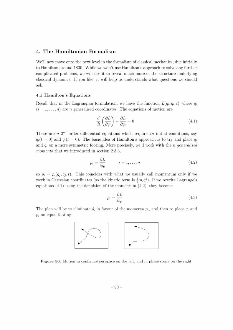
Figure 50: Motion in configuration space on the left, and in phase space on the right.
– 80 –
Let’s start by thinking pictorially. Recall that {qi
} defines a point in n-dimensional
configuration space C. Time evolution is a path in C. However, the state of the system
is defined by {qi
} and {pi
} in the sense that this information will allow us to determine
the state at all times in the future. The pair {qi
, pi
} defines a point in 2n-dimensional
phase space. Note that since a point in phase space is su�cient to determine the future
evolution of the system, paths in phase space can never cross. We say that evolution
is governed by a flow in phase space.
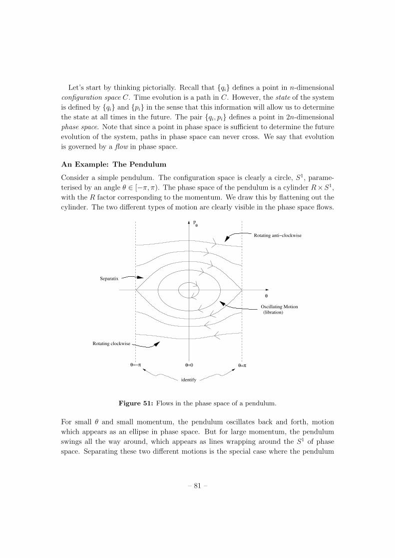
An Example: The Pendulum
Consider a simple pendulum. The configuration space is clearly a circle, S1, parame-
terised by an angle ✓ 2 [�⇡, ⇡). The phase space of the pendulum is a cylinder R⇥S1,
with the R factor corresponding to the momentum. We draw this by flattening out the
cylinder. The two di↵erent types of motion are clearly visible in the phase space flows.
θ=0
pθ
θ=πθ=−π
identify
θ
Oscillating Motion(libration)
Rotating anti−clockwise
Rotating clockwise
Separatix
Figure 51: Flows in the phase space of a pendulum.
For small ✓ and small momentum, the pendulum oscillates back and forth, motion
which appears as an ellipse in phase space. But for large momentum, the pendulum
swings all the way around, which appears as lines wrapping around the S1 of phase
space. Separating these two di↵erent motions is the special case where the pendulum
– 81 –
starts upright, falls, and just makes it back to the upright position. This curve in phase
space is called the separatix.
4.1.1 The Legendre Transform
We want to find a function on phase space that will determine the unique evolution
of qi
and pi
. This means it should be a function of qi
and pi
(and not of qi
) but must
contain the same information as the Lagrangian L(qi
, qi
, t). There is a mathematical
trick to do this, known as the Legendre transform.
To describe this, consider an arbitrary function f(x, y) so that the total derivative is
df =@f
@xdx+
@f
@ydy (4.4)
Now define a function g(x, y, u) = ux � f(x, y) which depends on three variables, x, y
and also u. If we look at the total derivative of g, we have
dg = d(ux)� df = u dx+ x du� @f
@xdx� @f
@ydy (4.5)
At this point u is an independent variable. But suppose we choose it to be a specific
function of x and y, defined by
u(x, y) =@f
@x(4.6)
Then the term proportional to dx in (4.5) vanishes and we have
dg = x du� @f
@ydy (4.7)
Or, in other words, g is to be thought of as a function of u and y: g = g(u, y). If we
want an explicit expression for g(u, y), we must first invert (4.6) to get x = x(u, y) and
then insert this into the definition of g so that
g(u, y) = u x(u, y)� f(x(u, y), y) (4.8)
This is the Legendre transform. It takes us from one function f(x, y) to a di↵erent func-
tion g(u, y) where u = @f/@x. The key point is that we haven’t lost any information.
Indeed, we can always recover f(x, y) from g(u, y) by noting that
@g
@u
�
�
�
�
y
= x(u, y) and@g
@y
�
�
�
�
u
=@f
@y(4.9)
which assures us that the inverse Legendre transform f = (@g/@u)u� g takes us back
to the original function.
– 82 –
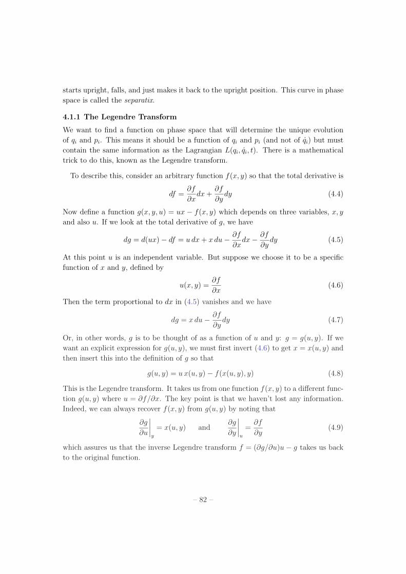
The geometrical meaning of the Legendre transform ux
f(x)
g(u)
x
Figure 52:
is captured in the diagram. For fixed y, we draw the two
curves f(x, y) and ux. For each slope u, the value of g(u)
is the maximal distance between the two curves. To see
this, note that extremising this distance means
d
dx(ux� f(x)) = 0 ) u =
@f
@x(4.10)
This picture also tells us that we can only apply the Legen-
dre transform to convex functions for which this maximum
exists. Now, armed with this tool, let’s return to dynamics.
4.1.2 Hamilton’s Equations
The Lagrangian L(qi
, qi
, t) is a function of the coordinates qi
, their time derivatives qi
and (possibly) time. We define the Hamiltonian to be the Legendre transform of the
Lagrangian with respect to the qi
variables,
H(qi
, pi
, t) =n
X
i=1
pi
qi
� L(qi
, qi
, t) (4.11)
where qi
is eliminated from the right hand side in favour of pi
by using
pi
=@L
@qi
= pi
(qj
, qj
, t) (4.12)
and inverting to get qi
= qi
(qj
, pj
, t). Now look at the variation of H:
dH = (dpi
qi
+ pi
dqi
)�✓
@L
@qi
dqi
+@L
@qi
dqi
+@L
@tdt
◆
= dpi
qi
� @L
@qi
dqi
� @L
@tdt (4.13)
but we know that this can be rewritten as
dH =@H
@qi
dqi
+@H
@pi
dpi
+@H
@tdt (4.14)
So we can equate terms. So far this is repeating the steps of the Legendre transform.
The new ingredient that we now add is Lagrange’s equation which reads pi
= @L/@qi
.
We find
pi
= �@H@q
i
qi
=@H
@pi
(4.15)
�@L@t
=@H
@t(4.16)
– 83 –
These are Hamilton’s equations. We have replaced n 2nd order di↵erential equations by
2n 1st order di↵erential equations for qi
and pi
. In practice, for solving problems, this
isn’t particularly helpful. But, as we shall see, conceptually it’s very useful!
4.1.3 Examples
1) A Particle in a Potential
Let’s start with a simple example: a particle moving in a potential in 3-dimensional
space. The Lagrangian is simply
L =1
2mr2 � V (r) (4.17)
We calculate the momentum by taking the derivative with respect to r
p =@L
@r= mr (4.18)
which, in this case, coincides with what we usually call momentum. The Hamiltonian
is then given by
H = p · r� L =1
2mp2 + V (r) (4.19)
where, in the end, we’ve eliminated r in favour of p and written the Hamiltonian as a
function of p and r. Hamilton’s equations are simply
r =@H
@p=
1
mp
p = �@H@r
= �rV (4.20)
which are familiar: the first is the definition of momentum in terms of velocity; the
second is Newton’s equation for this system.
2) A Particle in an Electromagnetic Field
We saw in section 2.5.7 that the Lagrangian for a charged particle moving in an elec-
tromagnetic field is
L = 1
2
mr2 � e (�� r ·A) (4.21)
From this we compute the momentum conjugate to the position
p =@L
@r= mr+ eA (4.22)
– 84 –
which now di↵ers from what we usually call momentum by the addition of the vector
potential A. Inverting, we have
r =1
m(p� eA) (4.23)
So we calculate the Hamiltonian to be
H(p, r) = p · r� L
=1
mp · (p� eA)�
1
2m(p� eA)2 � e�+
e
m(p� eA) ·A
�
=1
2m(p� eA)2 + e� (4.24)
Now Hamilton’s equations read
r =@H
@p=
1
m(p� eA) (4.25)
while the p = �@H/@r equation is best expressed in terms of components
pa
= �@H@r
a
= �e@�
@ra
+e
m(p
b
� eAb
)@A
b
@ra
(4.26)
To show that this is equivalent to the Lorentz force law requires some rearranging of
the indices, but it’s not too hard.
An Example of the Example
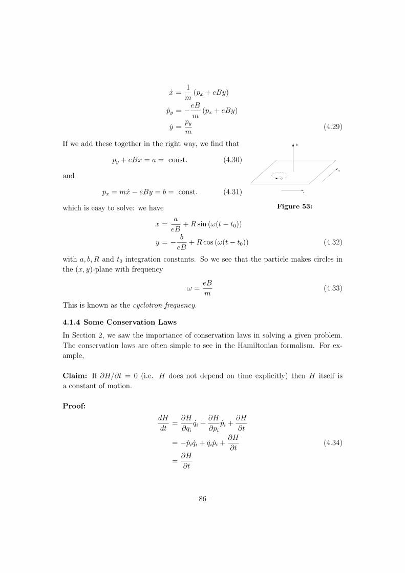
Let’s illustrate the dynamics of a particle moving in a magnetic field by looking at a
particular case. Imagine a uniform magnetic field pointing in the z-direction: B =
(0, 0, B). We can get this from a vector potential B = r⇥A with
A = (�By, 0, 0) (4.27)
This vector potential isn’t unique: we could choose others related by a gauge transform
as described in section 2.5.7. But this one will do for our purposes. Consider a particle
moving in the (x, y)-plane. Then the Hamiltonian for this system is
H =1
2m(p
x
+ eBy)2 +1
2mp2y
(4.28)
From which we have four, first order di↵erential equations which are Hamilton’s equa-
tions
px
= 0
– 85 –
x =1
m(p
x
+ eBy)
py
= �eB
m(p
x
+ eBy)
y =py
m(4.29)
If we add these together in the right way, we find that
x
y
B
Figure 53:
py
+ eBx = a = const. (4.30)
and
px
= mx� eBy = b = const. (4.31)
which is easy to solve: we have
x =a
eB+R sin (!(t� t
0
))
y = � b
eB+R cos (!(t� t
0
)) (4.32)
with a, b, R and t0
integration constants. So we see that the particle makes circles in
the (x, y)-plane with frequency
! =eB
m(4.33)
This is known as the cyclotron frequency.
4.1.4 Some Conservation Laws
In Section 2, we saw the importance of conservation laws in solving a given problem.
The conservation laws are often simple to see in the Hamiltonian formalism. For ex-
ample,
Claim: If @H/@t = 0 (i.e. H does not depend on time explicitly) then H itself is
a constant of motion.
Proof:
dH
dt=@H
@qi
qi
+@H
@pi
pi
+@H
@t
= �pi
qi
+ qi
pi
+@H
@t(4.34)
=@H
@t
– 86 –
Claim: If an ignorable coordinate q doesn’t appear in the Lagrangian then, by con-
struction, it also doesn’t appear in the Hamiltonian. The conjugate momentum pq
is
then conserved.
Proof
pq
=@H
@q= 0 (4.35)
4.1.5 The Principle of Least Action
Recall that in section 2.1 we saw the principle of least action from the Lagrangian
perspective. This followed from defining the action
S =
Z
t2
t1
L(qi
, qi
, t) dt (4.36)
Then we could derive Lagrange’s equations by insisting that �S = 0 for all paths with
fixed end points so that �qi
(t1
) = �qi
(t2
) = 0. How does this work in the Hamiltonian
formalism? It’s quite simple! We define the action
S =
Z
t2
t1
(pi
qi
�H)dt (4.37)
where, of course, qi
= qi
(qi
, pi
). Now we consider varying qi
and pi
independently. Notice
that this is di↵erent from the Lagrangian set-up, where a variation of qi
automatically
leads to a variation of qi
. But remember that the whole point of the Hamiltonian
formalism is that we treat qi
and pi
on equal footing. So we vary both. We have
�S =
Z
t2
t1
⇢
�pi
qi
+ pi
�qi
� @H
@pi
�pi
� @H
@qi
�qi
�
dt
=
Z
t2
t1
⇢
qi
� @H
@pi
�
�pi
+
�pi
� @H
@qi
�
�qi
�
dt+ [pi
�qi
]t2t1
(4.38)
and there are Hamilton’s equations waiting for us in the square brackets. If we look
for extrema �S = 0 for all �pi
and �qi
we get Hamilton’s equations
qi
=@H
@pi
and pi
= �@H@q
i
(4.39)
Except there’s a very slight subtlety with the boundary conditions. We need the last
term in (4.38) to vanish, and so require only that
�qi
(t1
) = �qi
(t2
) = 0 (4.40)
– 87 –
while �pi
can be free at the end points t = t1
and t = t2
. So, despite our best e↵orts,
qi
and pi
are not quite symmetric in this formalism.
Note that we could simply impose �pi
(t1
) = �pi
(t2
) = 0 if we really wanted to and
the above derivation still holds. It would mean we were being more restrictive on the
types of paths we considered. But it does have the advantage that it keeps qi
and pi
on a symmetric footing. It also means that we have the freedom to add a function to
consider actions of the form
S =
Z
t2
t1
✓
pi
qi
�H(q, p) +dF (q, p)
dt
◆
(4.41)
so that what sits in the integrand di↵ers from the Lagrangian. For some situations this
may be useful.
4.1.6 William Rowan Hamilton (1805-1865)
The formalism described above arose out of Hamilton’s interest in the theory of optics.
The ideas were published in a series of books entitled “Theory of Systems of Rays”, the
first of which appeared while Hamilton was still an undergraduate at Trinity College,
Dublin. They also contain the first application of the Hamilton-Jacobi formulation
(which we shall see in Section 4.7) and the first general statement of the principal of
least action, which sometimes goes by the name of “Hamilton’s Principle”.
Hamilton’s genius was recognised early. His capacity to soak up classical languages
and to find errors in famous works of mathematics impressed many. In an unprece-
dented move, he was o↵ered a full professorship in Dublin while still an undergraduate.
He also held the position of “Royal Astronomer of Ireland”, allowing him to live at
Dunsink Observatory even though he rarely did any observing. Unfortunately, the
later years of Hamilton’s life were not happy ones. The woman he loved married an-
other and he spent much time depressed, mired in drink, bad poetry and quaternions.
4.2 Liouville’s Theorem
We’ve succeeded in rewriting classical dynamics in terms of first order di↵erential equa-
tions in which each point in phase space follows a unique path under time evolution.
We speak of a flow on phase space. In this section, we’ll look at some of the properties
of these flows
Liouville’s Theorem: Consider a region in phase space and watch it evolve over
time. Then the shape of the region will generically change, but Liouville’s theorem
states that the volume remains the same.
– 88 –
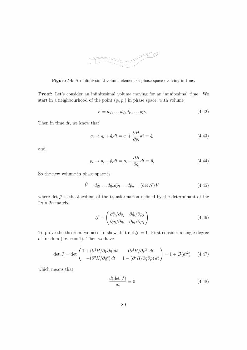
Figure 54: An infinitesimal volume element of phase space evolving in time.
Proof: Let’s consider an infinitesimal volume moving for an infinitesimal time. We
start in a neighbourhood of the point (qi
, pi
) in phase space, with volume
V = dq1
. . . dqn
dp1
. . . dpn
(4.42)
Then in time dt, we know that
qi
! qi
+ qi
dt = qi
+@H
@pi
dt ⌘ qi
(4.43)
and
pi
! pi
+ pi
dt = pi
� @H
@qi
dt ⌘ pi
(4.44)
So the new volume in phase space is
V = dq1
. . . dqn
dp1
. . . dpn
= (detJ )V (4.45)
where detJ is the Jacobian of the transformation defined by the determinant of the
2n⇥ 2n matrix
J =
@qi
/@qj
@qi
/@pj
@pi
/@qj
@pi
/@pj
!
(4.46)
To prove the theorem, we need to show that detJ = 1. First consider a single degree
of freedom (i.e. n = 1). Then we have
detJ = det
1 + (@2H/@p@q)dt (@2H/@p2) dt
�(@2H/@q2) dt 1� (@2H/@q@p) dt
!
= 1 +O(dt2) (4.47)
which means that
d(detJ )
dt= 0 (4.48)
– 89 –
so that the volume remains constant for all time. Now to generalise this to arbitrary
n, we have
detJ = det
�ij
+ (@2H/@pi
@qj
)dt (@2H/@pi
@pj
) dt
�(@2H/@qi
@qj
) dt �ij
� (@2H/@qi
@pj
) dt
!
(4.49)
To compute the determinant, we need the result that det(1+ ✏M) = 1+ ✏TrM +O(✏2)
for any matrix M and small ✏. Then we have
detJ = 1 +X
i
✓
@2H
@pi
@qi
� @2H
@qi
@pi
◆
dt+O(dt2) = 1 +O(dt2) (4.50)
and we’re done. ⇤
4.2.1 Liouville’s Equation
So how should we think about the volume of phase space? We could consider an
ensemble (or collection) of systems with some density function ⇢(p, q, t). We might
want to do this because
• We have a single system but don’t know the exact state very well. Then ⇢ is
understood as a probability parameterising our ignorance andZ
⇢(q, p, t)Y
i
dpi
dqi
= 1 (4.51)
• We may have a large number N of identical, non-interacting systems (e.g. N =
1023 gas molecules in a jar) and we really only care about the averaged behaviour.
Then the distribution ⇢ satisfiesZ
⇢(q, p, t)Y
i
dqi
dpi
= N (4.52)
In the latter case, we know that particles in phase space (i.e. dynamical systems)
are neither created nor destroyed, so the number of particles in a given “comoving” vol-
ume is conserved. Since Liouville tells us that the volume elements dpdq are preserved,
we have d⇢/dt = 0. We write this as
d⇢
dt=@⇢
@t+@⇢
@qi
qi
+@⇢
@pi
pi
=@⇢
@t+@⇢
@qi
@H
@pi
� @⇢
@pi
@H
@qi
= 0 (4.53)
– 90 –
Rearranging the terms, we have,
@⇢
@t=
@⇢
@pi
@H
@qi
� @⇢
@qi
@H
@pi
(4.54)
which is Liouville’s equation.
Notice that Liouville’s theorem holds whether or not the system conserves energy.
(i.e. whether or not @H/@t = 0). But the system must be described by a Hamiltonian.
For example, systems with dissipation typically head to regions of phase space with
qi
= 0 and so do not preserve phase space volume.
The central idea of Liouville’s theorem – that volume of phase space is constant –
is somewhat reminiscent of quantum mechanics. Indeed, this is the first of several oc-
casions where we shall see ideas of quantum physics creeping into the classical world.
Suppose we have a system of particles distributed randomly within a square �q�p in
phase space. Liouville’s theorem implies that if we evolve the system in any Hamil-
tonian manner, we can cut down the spread of positions of the particles only at the
cost of increasing the spread of momentum. We’re reminded strongly of Heisenberg’s
uncertainty relation, which is also written �q�p = constant.
While Liouville and Heisenberg seem to be talking the same language, there are very
profound di↵erences between them. The distribution in the classical picture reflects
our ignorance of the system rather than any intrinsic uncertainty. This is perhaps best
illustrated by the fact that we can evade Liouville’s theorem in a real system! The
crucial point is that a system of classical particles is really described by collection of
points in phase space rather than a continuous distribution ⇢(q, p) as we modelled it
above. This means that if we’re clever we can evolve the system with a Hamiltonian
so that the points get closer together, while the spaces between the points get pushed
away. A method for achieving this is known as stochastic cooling and is an important
part of particle collider technology. In 1984 van der Meer won the the Nobel prize for
pioneering this method.
4.2.2 Time Independent Distributions
Often in physics we’re interested in probability distributions that don’t change explicitly
in time (i.e. @⇢/@t = 0). There’s an important class of these of the form,
⇢ = ⇢(H(q, p)) (4.55)
To see that these are indeed time independent, look at
@⇢
@t=
@⇢
@pi
@H
@qi
� @⇢
@qi
@H
@pi
– 91 –
=@⇢
@H
@H
@pi
@H
@qi
� @⇢
@H
@H
@qi
@H
@pi
= 0 (4.56)
A very famous example of this type is the Boltzmann distribution
⇢ = exp
✓
�H(q, p)
kT
◆
(4.57)
for systems at a temperature T . Here k is the Boltzmann constant.
For example, for a free particle with H = p2/2m, the Boltzmann distribution is
⇢ = exp(�mr2/2kT ) which is a Gaussian distribution in velocities.
An historically more interesting example comes from looking at a free particle in a
magnetic field, so H = (p � eA)2/2m (where we’ve set the speed of light c = 1 for
simplicity). Then the Boltzmann distribution is
⇢ = exp
✓
�H(q, p)
kT
◆
= exp
✓
�mr2
2kT
◆
(4.58)
which is again a Gaussian distribution of velocities. In other words, the distribution
in velocities is independent of the magnetic field. But this is odd: the magnetism of
solids is all about how the motion of electrons is a↵ected by magnetic fields. Yet we’ve
seen that the magnetic field doesn’t a↵ect the velocities of electrons. This is known as
the Bohr-van Leeuwen paradox: there can be no magnetism in classical physics! This
was one of the motivations for the development of quantum theory.
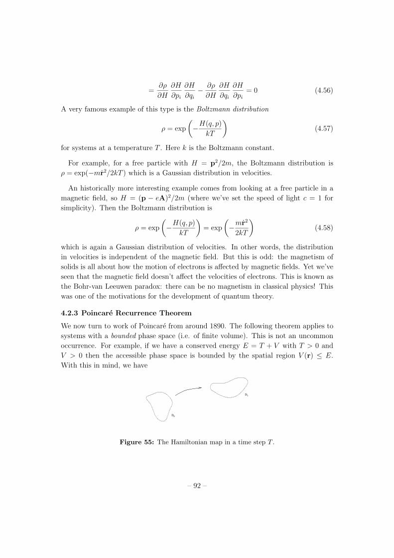
4.2.3 Poincare Recurrence Theorem
We now turn to work of Poincare from around 1890. The following theorem applies to
systems with a bounded phase space (i.e. of finite volume). This is not an uncommon
occurrence. For example, if we have a conserved energy E = T + V with T > 0 and
V > 0 then the accessible phase space is bounded by the spatial region V (r) E.
With this in mind, we have
D0
D1
Figure 55: The Hamiltonian map in a time step T .
– 92 –
Theorem: Consider an initial point P in phase space. Then for any neighbourhood
D0
of P , there exists a point P 0 2 D0
that will return to D0
in a finite time.
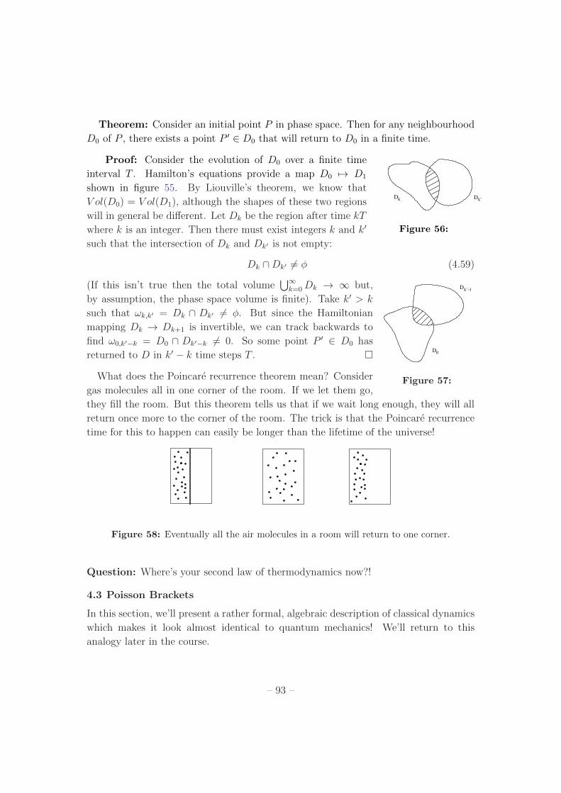
Proof: Consider the evolution of D0
over a finite time
kDk’D
Figure 56:
interval T . Hamilton’s equations provide a map D0
7! D1
shown in figure 55. By Liouville’s theorem, we know that
V ol(D0
) = V ol(D1
), although the shapes of these two regions
will in general be di↵erent. Let Dk
be the region after time kT
where k is an integer. Then there must exist integers k and k0
such that the intersection of Dk
and Dk
0 is not empty:
Dk
\Dk
0 6= � (4.59)
(If this isn’t true then the total volumeS1
k=0
Dk
! 1 but,k’−k
D
D0
Figure 57:
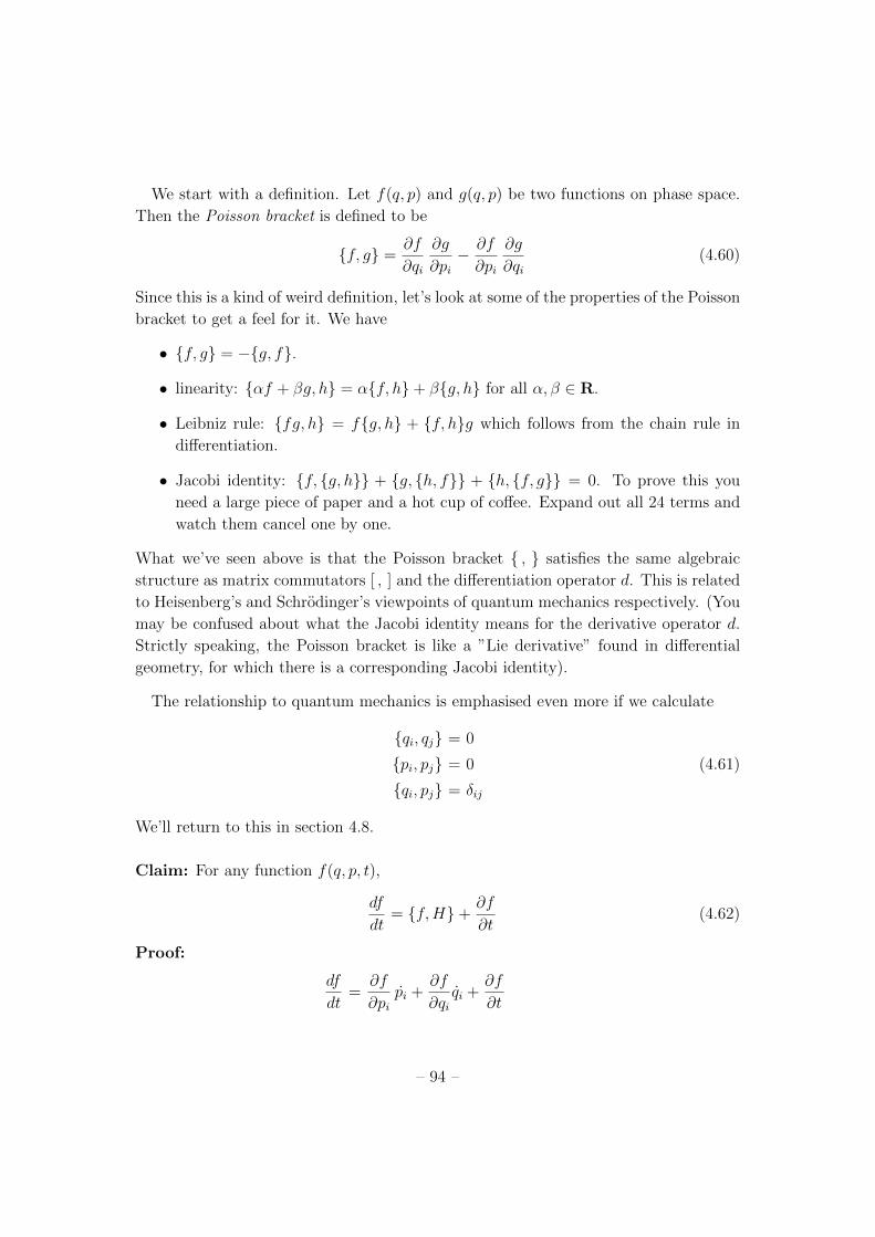
by assumption, the phase space volume is finite). Take k0 > k
such that !k,k
0 = Dk
\ Dk
0 6= �. But since the Hamiltonian
mapping Dk
! Dk+1
is invertible, we can track backwards to
find !0,k
0�k
= D0
\ Dk
0�k
6= 0. So some point P 0 2 D0
has
returned to D in k0 � k time steps T . ⇤
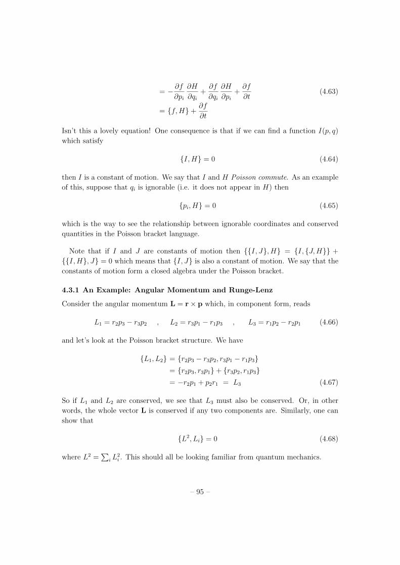
What does the Poincare recurrence theorem mean? Consider
gas molecules all in one corner of the room. If we let them go,
they fill the room. But this theorem tells us that if we wait long enough, they will all
return once more to the corner of the room. The trick is that the Poincare recurrence
time for this to happen can easily be longer than the lifetime of the universe!
Figure 58: Eventually all the air molecules in a room will return to one corner.
Question: Where’s your second law of thermodynamics now?!
4.3 Poisson Brackets
In this section, we’ll present a rather formal, algebraic description of classical dynamics
which makes it look almost identical to quantum mechanics! We’ll return to this
analogy later in the course.
– 93 –
We start with a definition. Let f(q, p) and g(q, p) be two functions on phase space.
Then the Poisson bracket is defined to be
{f, g} =@f
@qi
@g
@pi
� @f
@pi
@g
@qi
(4.60)
Since this is a kind of weird definition, let’s look at some of the properties of the Poisson
bracket to get a feel for it. We have
• {f, g} = �{g, f}.• linearity: {↵f + �g, h} = ↵{f, h}+ �{g, h} for all ↵, � 2 R.
• Leibniz rule: {fg, h} = f{g, h} + {f, h}g which follows from the chain rule in
di↵erentiation.
• Jacobi identity: {f, {g, h}} + {g, {h, f}} + {h, {f, g}} = 0. To prove this you
need a large piece of paper and a hot cup of co↵ee. Expand out all 24 terms and
watch them cancel one by one.
What we’ve seen above is that the Poisson bracket { , } satisfies the same algebraic
structure as matrix commutators [ , ] and the di↵erentiation operator d. This is related
to Heisenberg’s and Schrodinger’s viewpoints of quantum mechanics respectively. (You
may be confused about what the Jacobi identity means for the derivative operator d.
Strictly speaking, the Poisson bracket is like a ”Lie derivative” found in di↵erential
geometry, for which there is a corresponding Jacobi identity).
The relationship to quantum mechanics is emphasised even more if we calculate
{qi
, qj
} = 0
{pi
, pj
} = 0 (4.61)
{qi
, pj
} = �ij
We’ll return to this in section 4.8.
Claim: For any function f(q, p, t),
df
dt= {f,H}+ @f
@t(4.62)
Proof:
df
dt=
@f
@pi
pi
+@f
@qi
qi
+@f
@t
– 94 –
= � @f
@pi
@H
@qi
+@f
@qi
@H
@pi
+@f
@t(4.63)
= {f,H}+ @f
@t
Isn’t this a lovely equation! One consequence is that if we can find a function I(p, q)
which satisfy
{I,H} = 0 (4.64)
then I is a constant of motion. We say that I and H Poisson commute. As an example
of this, suppose that qi
is ignorable (i.e. it does not appear in H) then
{pi
, H} = 0 (4.65)
which is the way to see the relationship between ignorable coordinates and conserved
quantities in the Poisson bracket language.
Note that if I and J are constants of motion then {{I, J}, H} = {I, {J,H}} +
{{I,H}, J} = 0 which means that {I, J} is also a constant of motion. We say that the
constants of motion form a closed algebra under the Poisson bracket.
4.3.1 An Example: Angular Momentum and Runge-Lenz
Consider the angular momentum L = r⇥ p which, in component form, reads
L1
= r2
p3
� r3
p2
, L2
= r3
p1
� r1
p3
, L3
= r1
p2
� r2
p1
(4.66)
and let’s look at the Poisson bracket structure. We have
{L1
, L2
} = {r2
p3
� r3
p2
, r3
p1
� r1
p3
}= {r
2
p3
, r3
p1
}+ {r3
p2
, r1
p3
}= �r
2
p1
+ p2
r1
= L3
(4.67)
So if L1
and L2
are conserved, we see that L3
must also be conserved. Or, in other
words, the whole vector L is conserved if any two components are. Similarly, one can
show that
{L2, Li
} = 0 (4.68)
where L2 =P
i
L2
i
. This should all be looking familiar from quantum mechanics.
– 95 –
Another interesting object is the (Hermann-Bernoulli-Laplace-Pauli-) Runge-Lenz
vector, defined as
A =1
mp⇥ L� r (4.69)
where r = r/r. This vector satisfies A · L = 0. If you’re willing to spend some time
playing with indices, it’s not hard to derive the following expressions for the Poisson
bracket structure
{La
, Ab
} = ✏abc
Ac
, {Aa
, Ab
} = � 2
m
✓
p2
2m� 1
r
◆
✏abc
Lc
(4.70)
The last of these equations suggests something special might happen when we consider
the familiar Hamiltonian H = p2/2m� 1/r so that the Poisson bracket becomes
{Aa
, Ab
} = �2H
m✏abc
Lc
(4.71)
Indeed, for this choice of Hamiltonian is a rather simple to show that
{H,A} = 0 (4.72)
So we learn that the Hamiltonian with �1/r potential has another constant of motionA
that we’d previously missed! The fact that A is conserved can be used to immediately
derive Kepler’s elliptical orbits: dotting A with r yields r ·A+ 1 = L2/r which is the
equation for an ellipse. Note that the three constants of motion, L, A and H form a
closed algebra under the Poisson bracket.
Noether’s theorem tells us that the conservation of L and H are related to rotational
symmetry and time translation respectively. One might wonder whether there’s a
similar symmetry responsible for the conservation of A. It turns out that there is: the
Hamiltonian has a hidden SO(4) symmetry group. You can read more about this in
Goldstein.
4.3.2 An Example: Magnetic Monopoles
We’ve seen in the example of section 4.1.3 that a particle in a magnetic field B = r⇥A
is described by the Hamiltonian
H =1
2m(p� eA(r))2 =
m
2r2 (4.73)
where, as usual in the Hamiltonian, r is to be thought of as a function of r and p. It’s
a simple matter to compute the Poisson bracket structure for this system: it reads
{mra
,mrb
} = e ✏abc
Bc
, {mra
, rb
} = ��ab
(4.74)
– 96 –
Let’s now use this to describe a postulated object known as a magnetic monopole. It’s
a fact that all magnets ever discovered are dipoles: they have both a north and south
pole. Chop the magnet in two, and each piece also has a north and a south pole.
Indeed, this fact is woven into the very heart of electromagnetism when formulated in
terms of the gauge potential A. Since we define B = r⇥A, we immediately have one
of Maxwell’s equations,
r ·B = 0 (4.75)
which states that any flux that enters a region must also leave. Or, in other words,
there can be no magnetic monopole. Such a monopole would have a radial magnetic
field,
B = gr
r3(4.76)
which doesn’t satisfy (4.75) since it gives rise to a delta function on the right-hand side.
So if magnetic monopoles have never been observed, and are forbidden by Maxwell’s
equations, why are we interested in them?! The point is that every theory that goes
beyond Maxwell’s equations and tries to unify electromagnetism with the other forces
of Nature predicts magnetic monopoles. So there’s reason to suspect that, somewhere
in the universe, there may be particles with a radial magnetic field given by (4.76).
What happens if an electron moves in the background of a monopole? It’s tricky
to set up the Lagrangian as we don’t have a gauge potential A. (Actually, one can
work with certain singular gauge potentials but we won’t go there). However, we can
play with the Poisson brackets (4.74) which contain only the magnetic field. As an
application, consider the generalised angular momentum,
J = mr⇥ r� ger (4.77)
where r = r/r. For g = 0, this expression reduces to the usual angular momentum. It is
a simple matter to show using (4.74) that in the background of the magnetic monopole
the Hamiltonian H = 1
2
mr2 and J satisfy
{H,J} = 0 (4.78)
which guarantees that J is a constant of motion. What do we learn from this? Since
J is conserved, we can look at r · J = �eg to learn that the motion of an electron in
the background of a magnetic monopole lies on a cone of angle cos ✓ = eg/J pointing
away from the vector J.
– 97 –
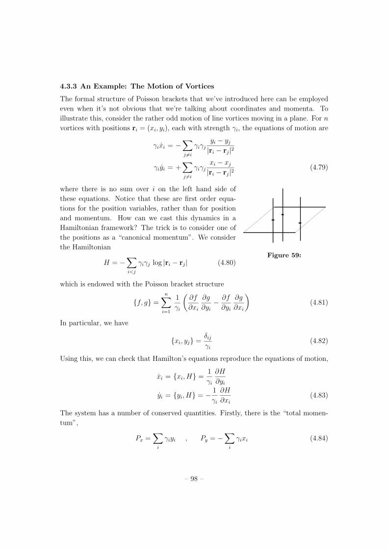
4.3.3 An Example: The Motion of Vortices
The formal structure of Poisson brackets that we’ve introduced here can be employed
even when it’s not obvious that we’re talking about coordinates and momenta. To
illustrate this, consider the rather odd motion of line vortices moving in a plane. For n
vortices with positions ri
= (xi
, yi
), each with strength �i
, the equations of motion are
�i
xi
= �X
j 6=i
�i
�j
yi
� yj
|ri
� rj
|2
�i
yi
= +X
j 6=i
�i
�j
xi
� xj
|ri
� rj
|2 (4.79)
where there is no sum over i on the left hand side of
Figure 59:
these equations. Notice that these are first order equa-
tions for the position variables, rather than for position
and momentum. How can we cast this dynamics in a
Hamiltonian framework? The trick is to consider one of
the positions as a “canonical momentum”. We consider
the Hamiltonian
H = �X
i<j
�i
�j
log |ri
� rj
| (4.80)
which is endowed with the Poisson bracket structure
{f, g} =n
X
i=1
1
�i
✓
@f
@xi
@g
@yi
� @f
@yi
@g
@xi
◆
(4.81)
In particular, we have
{xi
, yj
} =�ij
�i
(4.82)
Using this, we can check that Hamilton’s equations reproduce the equations of motion,
xi
= {xi
, H} =1
�i
@H
@yi
yi
= {yi
, H} = � 1
�i
@H
@xi
(4.83)
The system has a number of conserved quantities. Firstly, there is the “total momen-
tum”,
Px
=X
i
�i
yi
, Py
= �X
i
�i
xi
(4.84)
– 98 –
which satisfy {Px
, H} = {Py
, H} = 0, ensuring that they are conserved quantities.
We also have {Px
, Py
} =P
i
�i
and the right hand side, being constant, is trivially
conserved.
The other conserved quantity is the “total angular momentum”,
J = �1
2
n
X
i=1
�i
(x2
i
+ y2i
) (4.85)
which again satisfies {J,H} = 0, ensuring it is conserved. The full algebra of the
conserved quantities includes {Px
, J} = �Py
and {Py
, J} = Px
, so the system closes
(meaning we get back something we know on the right hand side). In fact, one can
show that H, J and (P 2
x
+ P 2
y
) provide three mutually Poisson commuting conserved
quantities.
So what is the resulting motion of a bunch of vortices? For two vortices, we can
simply solve the equations of motion to find,
x1
� x2
= R sin⇣ !
R2
(t� t0
)⌘
y1
� y2
= R cos⇣ !
R2
(t� t0
)⌘
(4.86)
where R is the separation between the vortices and ! = (�1
+ �2
)/R2. So we learn
that two vortices orbit each other with frequency inversely proportional to the square
of their separation.
For three vortices, it turns out that there is a known solution which is possible
because of the three mutually Poisson commuting conserved quantities we saw above.
We say the system is “integrable”. We’ll define this properly shortly. For four or more
vortices, the motion is chaotic5.
You may think that the Poisson bracket structure {x, y} 6= 0 looks a little strange.
But it also appears in a more familiar setting: a charged particle moving in a magnetic
field B = (0, 0, B). We saw this example in section 4.1.3, where we calculated
px
= mx� eB
mcy (4.87)
For large magnetic fields the second term in this equation dominates, and we have
px
⇡ �eBy/mc. In this case the Poisson bracket is
{x, px
} = 1 ) {x, y} ⇡ �mc
eB(4.88)
5For more details on this system, see the review H. Aref, “Integrable, Chaotic, and Turbulent VortexMotion in Two-Dimensional Flows”, Ann. Rev. Fluid Mech. 15 345 (1983).
– 99 –
This algebraic similarity between vortices and electrons is a hot topic of current re-
search: can we make vortices do similar things to electrons in magnetic fields? For
example: will vortices in a Bose-Einstein condensate form a fractional quantum Hall
state? This is currently an active area of research.
4.4 Canonical Transformations
There is a way to write Hamilton’s equations so that they look even more symmetric.
Define the 2n vector x = (q1
, . . . , qn
, p1
, . . . , pn
)T and the 2n⇥ 2n matrix J ,
J =
0 1
�1 0
!
(4.89)
where each entry is itself an n⇥nmatrix. Then with this notation, Hamilton’s equations
read
x = J@H
@x(4.90)
Now remember that in the Lagrangian formalism we made a big deal about the fact that
we could change coordinates qi
! Qi
(q) without changing the form of the equations.
Since we’ve managed to put qi
and pi
on an equal footing in the Hamiltonian formalism,
one might wonder if its possible to make an even larger class of transformations of the
form,
qi
! Qi
(q, p) and pi
! Pi
(q, p) (4.91)
The answer is yes! But not all such transformations are allowed. To see what class of
transformations leaves Hamilton’s equations invariant, we use our new symmetric form
in terms of x and write the transformation as
xi
! yi
(x) (4.92)
Note that we’ll continue to use the index i which now runs over the range i = 1, . . . , 2n.
We have
yi
=@y
i
@xj
xj
=@y
i
@xj
Jjk
@H
@yl
@yl
@xk
(4.93)
or, collating all the indices, we have
y = (J J J T )@H
@y(4.94)
– 100 –
where Jij
= @yi
/@xj
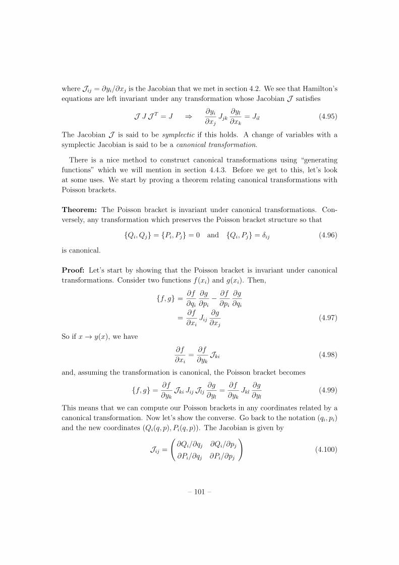
is the Jacobian that we met in section 4.2. We see that Hamilton’s
equations are left invariant under any transformation whose Jacobian J satisfies
J J J T = J ) @yi
@xj
Jjk
@yl
@xk
= Jil
(4.95)
The Jacobian J is said to be symplectic if this holds. A change of variables with a
symplectic Jacobian is said to be a canonical transformation.
There is a nice method to construct canonical transformations using “generating
functions” which we will mention in section 4.4.3. Before we get to this, let’s look
at some uses. We start by proving a theorem relating canonical transformations with
Poisson brackets.
Theorem: The Poisson bracket is invariant under canonical transformations. Con-
versely, any transformation which preserves the Poisson bracket structure so that
{Qi
, Qj
} = {Pi
, Pj
} = 0 and {Qi
, Pj
} = �ij
(4.96)
is canonical.
Proof: Let’s start by showing that the Poisson bracket is invariant under canonical
transformations. Consider two functions f(xi
) and g(xi
). Then,
{f, g} =@f
@qi
@g
@pi
� @f
@pi
@g
@qi
=@f
@xi
Jij
@g
@xj
(4.97)
So if x ! y(x), we have
@f
@xi
=@f
@yk
Jki
(4.98)
and, assuming the transformation is canonical, the Poisson bracket becomes
{f, g} =@f
@yk
Jki
Jij
Jlj
@g
@yl
=@f
@yk
Jkl
@g
@yl
(4.99)
This means that we can compute our Poisson brackets in any coordinates related by a
canonical transformation. Now let’s show the converse. Go back to the notation (qi
, pi
)
and the new coordinates (Qi
(q, p), Pi
(q, p)). The Jacobian is given by
Jij
=
@Qi
/@qj
@Qi
/@pj
@Pi
/@qj
@Pi
/@pj
!
(4.100)
– 101 –
If we now compute J JJ T in components, we get
(J JJ T )ij
=
{Qi
, Qj
} {Qi
, Pj
}{P
i
, Qj
} {Pi
, Pj
}
!
(4.101)
So whenever the Poisson bracket structure is preserved, the transformation is canonical.
⇤
Example
In the next section we’ll see several non-trivial examples of canonical transformations
which mix up q and p variables. But for now let’s content ourselves with reproducing
the coordinate changes that we had in section 2. Consider a change of coordinates of
the form
qi
! Qi
(q) (4.102)
We know that Lagrange’s equations are invariant under this. But what transformation
do we have to make on the momenta
pi
! Pi
(q, p) (4.103)
so that Hamilton’s equations are also invariant? We write ⇥ij
= @Qi
/@qj
and look at
the Jacobian
Jij
=
⇥ij
0
@Pi
/@qj
@Pi
/@pj
!
(4.104)
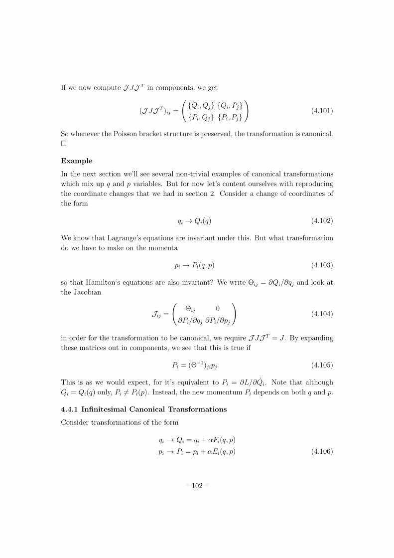
in order for the transformation to be canonical, we require J JJ T = J . By expanding
these matrices out in components, we see that this is true if
Pi
= (⇥�1)ji
pj
(4.105)
This is as we would expect, for it’s equivalent to Pi
= @L/@Qi
. Note that although
Qi
= Qi
(q) only, Pi
6= Pi
(p). Instead, the new momentum Pi
depends on both q and p.
4.4.1 Infinitesimal Canonical Transformations
Consider transformations of the form
qi
! Qi
= qi
+ ↵Fi
(q, p)
pi
! Pi
= pi
+ ↵Ei
(q, p) (4.106)
– 102 –
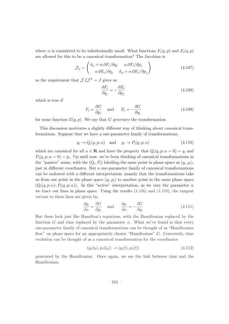
where ↵ is considered to be infinitesimally small. What functions Fi
(q, p) and Ei
(q, p)
are allowed for this to be a canonical transformation? The Jacobian is
Jij
=
�ij
+ ↵ @Fi
/@qj
↵ @Fi
/@pj
↵ @Ei
/@qj
�ij
+ ↵ @Ei
/@pj
!
(4.107)
so the requirement that J JJ T = J gives us
@Fi
@qj
= �@Ei
@pj
(4.108)
which is true if
Fi
=@G
@pi
and Ei
= �@G@q
i
(4.109)
for some function G(q, p). We say that G generates the transformation.
This discussion motivates a slightly di↵erent way of thinking about canonical trans-
formations. Suppose that we have a one-parameter family of transformations,
qi
! Qi
(q, p;↵) and pi
! Pi
(q, p;↵) (4.110)
which are canonical for all ↵ 2 R and have the property that Qi
(q, p;↵ = 0) = qi
and
Pi
(q, p;↵ = 0) = pi
. Up until now, we’ve been thinking of canonical transformations in
the “passive” sense, with the (Qi
, Pi
) labelling the same point in phase space as (qi
, pi
),
just in di↵erent coordinates. But a one-parameter family of canonical transformations
can be endowed with a di↵erent interpretation, namely that the transformations take
us from one point in the phase space (qi
, pi
) to another point in the same phase space
(Qi
(q, p;↵), Pi
(q, p;↵)). In this “active” interpretation, as we vary the parameter ↵
we trace out lines in phase space. Using the results (4.106) and (4.109), the tangent
vectors to these lines are given by,
dqi
d↵=@G
@pi
anddp
i
d↵= �@G
@qi
(4.111)
But these look just like Hamilton’s equations, with the Hamiltonian replaced by the
function G and time replaced by the parameter ↵. What we’ve found is that every
one-parameter family of canonical transformations can be thought of as “Hamiltonian
flow” on phase space for an appropriately chosen “Hamiltonian” G. Conversely, time
evolution can be thought of as a canonical transformation for the coordinates
(qi
(t0
), pi
(t0
)) ! (qi
(t), pi
(t)) (4.112)
generated by the Hamiltonian. Once again, we see the link between time and the
Hamiltonian.
– 103 –
As an example, consider the function G = pk
. Then the corresponding infinitesimal
canonical transformation is qi
! qi
+ ↵�ik
and pi
! pi
, which is simply a translation.
We say that translations of qk
are generated by the conjugate momentum G = pk
.
4.4.2 Noether’s Theorem Revisited
Recall that in the Lagrangian formalism, we saw a connection between symmetries and
conservation laws. How does this work in the Hamiltonian formulation?
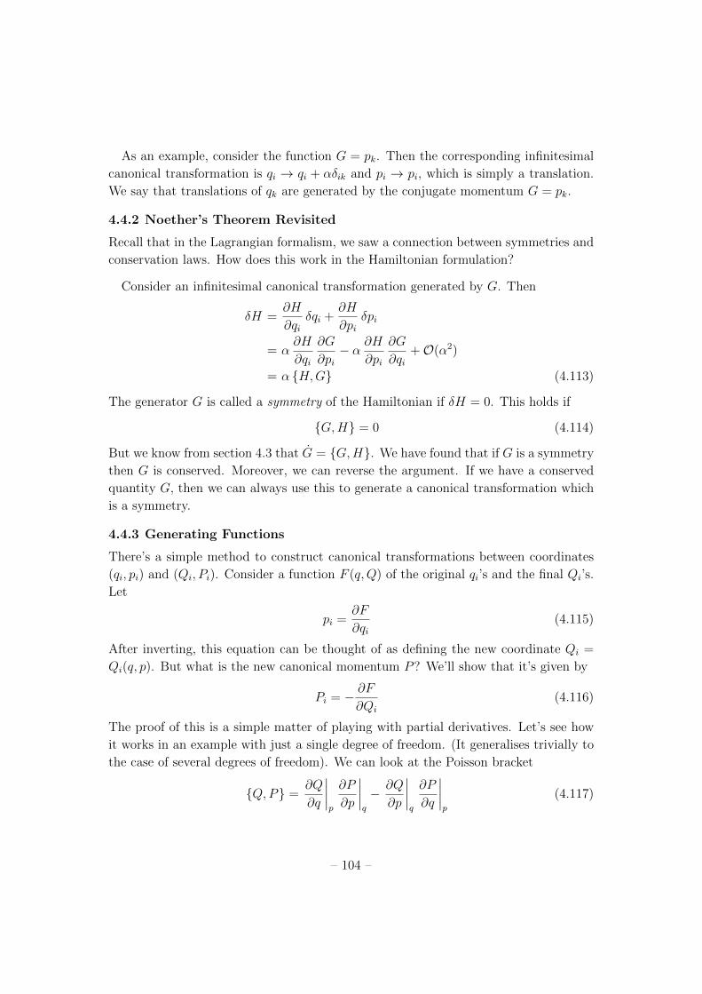
Consider an infinitesimal canonical transformation generated by G. Then
�H =@H
@qi
�qi
+@H
@pi
�pi
= ↵@H
@qi
@G
@pi
� ↵@H
@pi
@G
@qi
+O(↵2)
= ↵ {H,G} (4.113)
The generator G is called a symmetry of the Hamiltonian if �H = 0. This holds if
{G,H} = 0 (4.114)
But we know from section 4.3 that G = {G,H}. We have found that if G is a symmetry
then G is conserved. Moreover, we can reverse the argument. If we have a conserved
quantity G, then we can always use this to generate a canonical transformation which
is a symmetry.
4.4.3 Generating Functions
There’s a simple method to construct canonical transformations between coordinates
(qi
, pi
) and (Qi
, Pi
). Consider a function F (q,Q) of the original qi
’s and the final Qi
’s.
Let
pi
=@F
@qi
(4.115)
After inverting, this equation can be thought of as defining the new coordinate Qi
=
Qi
(q, p). But what is the new canonical momentum P? We’ll show that it’s given by
Pi
= � @F
@Qi
(4.116)
The proof of this is a simple matter of playing with partial derivatives. Let’s see how
it works in an example with just a single degree of freedom. (It generalises trivially to
the case of several degrees of freedom). We can look at the Poisson bracket
{Q,P} =@Q
@q
�
�
�
�
p
@P
@p
�
�
�
�
q
� @Q
@p
�
�
�
�
q
@P
@q
�
�
�
�
p
(4.117)
– 104 –
At this point we need to do the playing with partial derivatives. Equation (4.116)
defines P = P (q,Q), so we have
@P
@p
�
�
�
�
q
=@Q
@p
�
�
�
�
q
@P
@Q
�
�
�
�
q
and@P
@q
�
�
�
�
p
=@P
@q
�
�
�
�
Q
+@Q
@q
�
�
�
�
p
@P
@Q
�
�
�
�
q
(4.118)
Inserting this into the Poisson bracket gives
{Q,P} = � @Q
@p
�
�
�
�
q
@P
@q
�
�
�
�
Q
=@Q
@p
�
�
�
�
q
@2F
@q@Q=@Q
@p
�
�
�
�
q
@p
@Q
�
�
�
�
q
= 1 (4.119)
as required. The function F (q,Q) is known as a generating function of the first kind.
There are three further types of generating function, related to the first by Leg-
endre transforms. Each is a function of one of the original coordinates and one of
the new coordinates. You can check that the following expression all define canonical
transformations:
F2
(q, P ) : pi
=@F
2
@qi
and Qi
=@F
2
@Pi
(4.120)
F3
(p,Q) : qi
= �@F3
@pi
and Pi
= �@F3
@Qi
F4
(p, P ) : qi
= �@F4
@pi
and Qi
=@F
4
@Pi
4.5 Action-Angle Variables
We’ve all tried to solve problems in physics using the wrong coordinates and seen
what a mess it can be. If you work in Cartesian coordinates when the problem really
requires, say, spherical polar coordinates, it’s always possible to get to the right answer
with enough perseverance, but you’re really making life hard for yourself. The ability
to change coordinate systems can drastically simplify a problem. Now we have a much
larger set of transformations at hand; we can mix up q’s and p’s. An obvious question
is: Is this useful for anything?! In other words, is there a natural choice of variables
which makes solving a given problem much easier. In many cases, there is. They’re
called “angle-action” variables.
4.5.1 The Simple Harmonic Oscillator
We’ll start this section by doing a simple example which will illustrate the main point.
We’ll then move on to the more general theory. The example we choose is the simple
harmonic oscillator. Notice that as our theory gets more abstract, our examples get
easier!
– 105 –
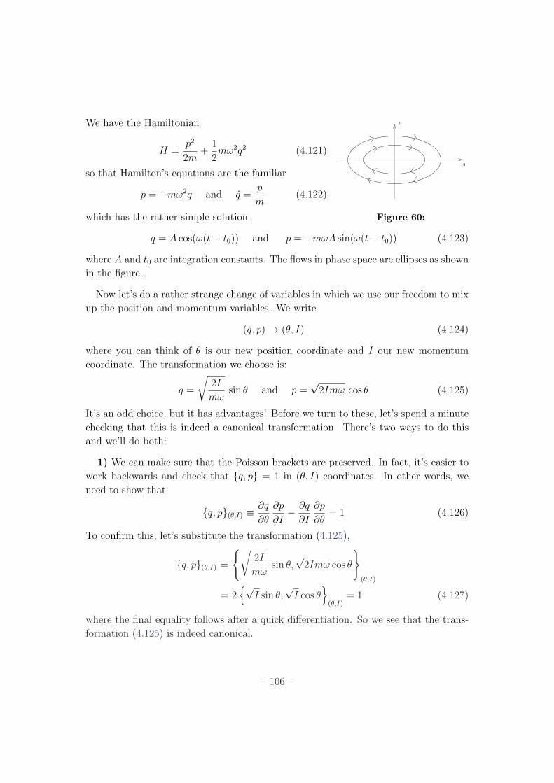
We have the Hamiltonian
q
p
Figure 60:
H =p2
2m+
1
2m!2q2 (4.121)
so that Hamilton’s equations are the familiar
p = �m!2q and q =p
m(4.122)
which has the rather simple solution
q = A cos(!(t� t0
)) and p = �m!A sin(!(t� t0
)) (4.123)
where A and t0
are integration constants. The flows in phase space are ellipses as shown
in the figure.
Now let’s do a rather strange change of variables in which we use our freedom to mix
up the position and momentum variables. We write
(q, p) ! (✓, I) (4.124)
where you can think of ✓ is our new position coordinate and I our new momentum
coordinate. The transformation we choose is:
q =
r
2I
m!sin ✓ and p =
p2Im! cos ✓ (4.125)
It’s an odd choice, but it has advantages! Before we turn to these, let’s spend a minute
checking that this is indeed a canonical transformation. There’s two ways to do this
and we’ll do both:
1) We can make sure that the Poisson brackets are preserved. In fact, it’s easier to
work backwards and check that {q, p} = 1 in (✓, I) coordinates. In other words, we
need to show that
{q, p}(✓,I)
⌘ @q
@✓
@p
@I� @q
@I
@p
@✓= 1 (4.126)
To confirm this, let’s substitute the transformation (4.125),
{q, p}(✓,I)
=
(
r
2I
m!sin ✓,
p2Im! cos ✓
)
(✓,I)
= 2np
I sin ✓,pI cos ✓
o
(✓,I)
= 1 (4.127)
where the final equality follows after a quick di↵erentiation. So we see that the trans-
formation (4.125) is indeed canonical.
– 106 –
2) The second way to see that the transformation is canonical is to prove that the
Jacobian is symplectic. Let’s now check it this way. We can calculate
J =
@✓/@q @✓/@p
@I/@q @I/@p
!
=
(m!/p) cos2 ✓ �(m!q/p2) cos2 ✓
m!q p/m!
!
(4.128)
from which we can calculate J JJ T and find that it is equal to J as required.
So we have a canonical transformation in (4.125). But what’s the point of doing
this? Let’s look at the Hamiltonian in our new variables.
H =1
2m(2m!I) sin2 ✓ +
1
2m!2
2I
m!cos2 ✓ = !I (4.129)
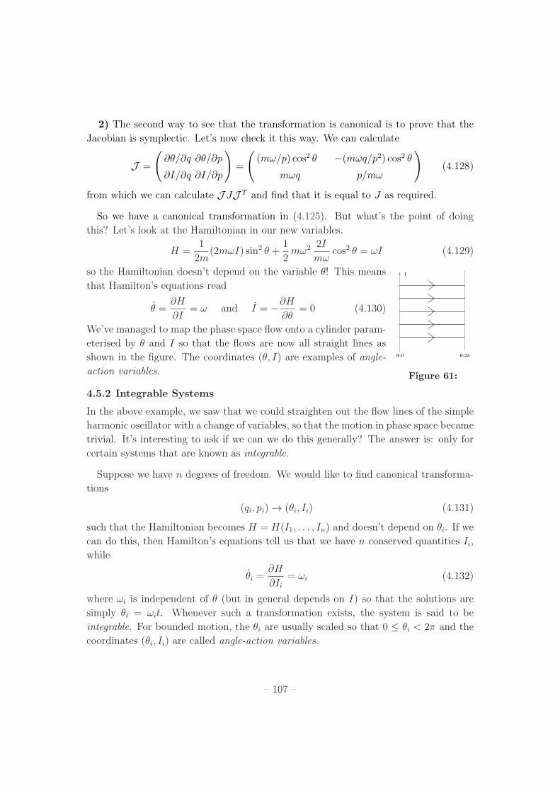
so the Hamiltonian doesn’t depend on the variable ✓! This means
θ=2πθ=0
I
Figure 61:
that Hamilton’s equations read
✓ =@H
@I= ! and I = �@H
@✓= 0 (4.130)
We’ve managed to map the phase space flow onto a cylinder param-
eterised by ✓ and I so that the flows are now all straight lines as
shown in the figure. The coordinates (✓, I) are examples of angle-
action variables.
4.5.2 Integrable Systems
In the above example, we saw that we could straighten out the flow lines of the simple
harmonic oscillator with a change of variables, so that the motion in phase space became
trivial. It’s interesting to ask if we can we do this generally? The answer is: only for
certain systems that are known as integrable.
Suppose we have n degrees of freedom. We would like to find canonical transforma-
tions
(qi
, pi
) ! (✓i
, Ii
) (4.131)
such that the Hamiltonian becomes H = H(I1
, . . . , In
) and doesn’t depend on ✓i
. If we
can do this, then Hamilton’s equations tell us that we have n conserved quantities Ii
,
while
✓i
=@H
@Ii
= !i
(4.132)
where !i
is independent of ✓ (but in general depends on I) so that the solutions are
simply ✓i
= !i
t. Whenever such a transformation exists, the system is said to be
integrable. For bounded motion, the ✓i
are usually scaled so that 0 ✓i
< 2⇡ and the
coordinates (✓i
, Ii
) are called angle-action variables.
– 107 –
Liouville’s Theorem on Integrable Systems: There is a converse statement.
If we can find n mutually Poisson commuting constants of motion I1
, . . . , In
then this
implies the existence of angle-action variables and the system is integrable. The re-
quirement of Poisson commutation {Ii
, Ij
} = 0 is the statement that we can view the
Ii
as canonical momentum variables. This is known as Liouville’s theorem. (Same
Liouville, di↵erent theorem). A proof can be found in the book by Arnold.
Don’t be fooled into thinking all systems are integrable. They are rather special and
precious. It remains an active area of research to find and study these systems. But
many – by far the majority – of systems are not integrable (chaotic systems notably
among them) and don’t admit this change of variables. Note that the question of
whether angle-action variables exist is a global one. Locally you can always straighten
out the flow lines; it’s a question of whether you can tie these straight lines together
globally without them getting tangled.
Clearly the motion of a completely integrable system is restricted to lie on Ii
=
constant slices of the phase space. A theorem in topology says that these surfaces must
be tori (S1 ⇥ . . .⇥ S1) known as the invariant tori.
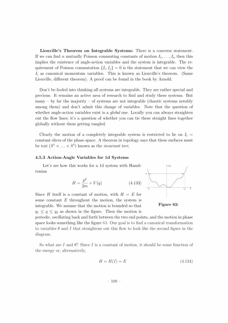
4.5.3 Action-Angle Variables for 1d Systems
Let’s see how this works for a 1d system with Hamil-
1q
2q
V(q)
q
E
Figure 62:
tonian
H =p2
2m+ V (q) (4.133)
Since H itself is a constant of motion, with H = E for
some constant E throughout the motion, the system is
integrable. We assume that the motion is bounded so that
q1
q q2
as shown in the figure. Then the motion is
periodic, oscillating back and forth between the two end points, and the motion in phase
space looks something like the figure 63. Our goal is to find a canonical transformation
to variables ✓ and I that straightens out this flow to look like the second figure in the
diagram.
So what are I and ✓? Since I is a constant of motion, it should be some function of
the energy or, alternatively,
H = H(I) = E (4.134)
– 108 –
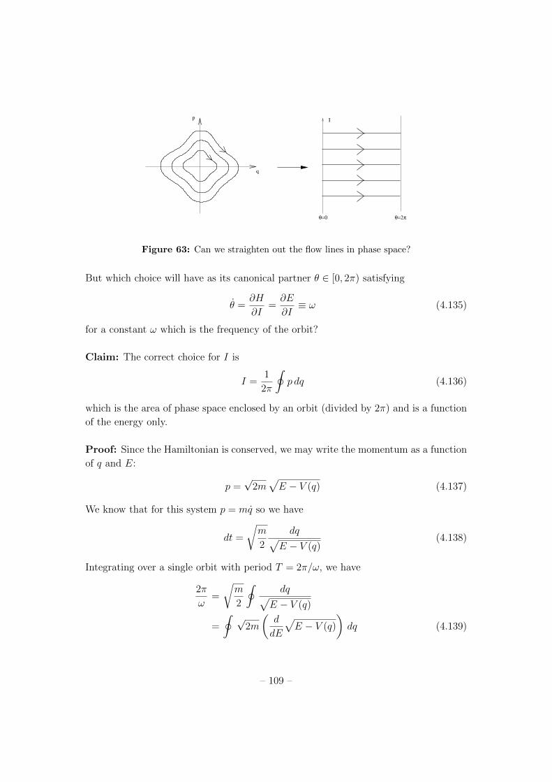
θ=2πθ=0
I
q
p
Figure 63: Can we straighten out the flow lines in phase space?
But which choice will have as its canonical partner ✓ 2 [0, 2⇡) satisfying
✓ =@H
@I=@E
@I⌘ ! (4.135)
for a constant ! which is the frequency of the orbit?
Claim: The correct choice for I is
I =1
2⇡
I
p dq (4.136)
which is the area of phase space enclosed by an orbit (divided by 2⇡) and is a function
of the energy only.
Proof: Since the Hamiltonian is conserved, we may write the momentum as a function
of q and E:
p =p2mp
E � V (q) (4.137)
We know that for this system p = mq so we have
dt =
r
m
2
dqp
E � V (q)(4.138)
Integrating over a single orbit with period T = 2⇡/!, we have
2⇡
!=
r
m
2
I
dqp
E � V (q)
=
I p2m
✓
d
dE
p
E � V (q)
◆
dq (4.139)
– 109 –
At this point we take the di↵erentiation d/dE outside the integral. This isn’t obviously
valid since the path around which the integral is evaluated itself changes with energy
E. Shortly we’ll show that this doesn’t matter. For now, let’s assume that this is valid
and continue to find
2⇡
!=
d
dE
I p2mp
E � V (q) dq
=d
dE
I
p dq
= 2⇡dI
dE(4.140)
where in the last line, we’ve substituted for our putative action variable I. Examining
our end result, we have found that I does indeed satisfy
dE
dI= ! (4.141)
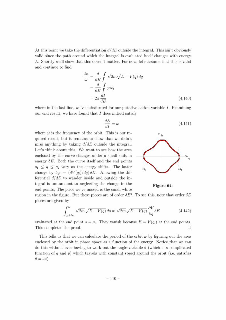
where ! is the frequency of the orbit. This is our re-
q
p
δq qδ1 2
Figure 64:
quired result, but it remains to show that we didn’t
miss anything by taking d/dE outside the integral.
Let’s think about this. We want to see how the area
enclosed by the curve changes under a small shift in
energy �E. Both the curve itself and the end points
q1
q q2
vary as the energy shifts. The latter
change by �qi
= (dV (qi
)/dq) �E. Allowing the dif-
ferential d/dE to wander inside and outside the in-
tegral is tantamount to neglecting the change in the
end points. The piece we’ve missed is the small white
region in the figure. But these pieces are of order �E2. To see this, note that order �E
pieces are given byZ
qi
qi+�qi
p2mp
E � V (q) dq ⇡p2mp
E � V (q)@V
@q�E (4.142)
evaluated at the end point q = qi
. They vanish because E = V (qi
) at the end points.
This completes the proof. ⇤
This tells us that we can calculate the period of the orbit ! by figuring out the area
enclosed by the orbit in phase space as a function of the energy. Notice that we can
do this without ever having to work out the angle variable ✓ (which is a complicated
function of q and p) which travels with constant speed around the orbit (i.e. satisfies
✓ = !t).
– 110 –
In fact, it’s not too hard to get an expression for ✓ by going over the above analysis
for a small part of the period. It follows from the above proof that
t =d
dE
Z
p dq (4.143)
but we want a ✓ which obeys ✓ = !t. We see that we can achieve this by taking the
choice
✓ = !d
dE
Z
p dq =dE
dI
d
dE
Z
p dq =d
dI
Z
p dq (4.144)
Because E is conserved, all 1d systems are integrable. What about higher dimen-
sional systems? If they are integrable, then there exists a change to angle-action vari-
ables given by
Ii
=1
2⇡
I
�i
X
j
pj
dqj
✓i
=@
@Ii
Z
�i
X
j
pj
dqj
(4.145)
where the �i
are the periods of the invariant tori.
4.5.4 Action-Angle Variables for the Kepler Problem
Perhaps the simplest integrable system with more than one degree of freedom is the
Kepler problem. This is a particle of mass m moving in three dimensions, subject to
the potential
V (r) = �k
r
We solved this already back in the Dynamics and Relativity course. Recall that we can
use the conservation of the (direction of) angular momentum to restrict dynamics to
a two-dimensional plane. We’ll work in polar coordinates (r,�) in this spatial plane.
The associated momenta are pr
= mr and p�
= mr2�. The Hamiltonian is
H =1
2mp2r
+1
2mr2p2�
� k
r(4.146)
There are two action variables, one associated to the radial motion and one associated
to the angular motion. The latter is straightforward: it is the angular momentum itself
I�
=1
2⇡
Z
2⇡
0
p�
d� = p�
– 111 –
The action variable for the radial motion is more interesting. We can calculating it
by using the fact that the total energy, E, and the angular momentum I�
are both
conserved. Then, rearranging (4.146), we have
p2r
= 2m
✓
E +k
r
◆
� I2�
r2
and the action variable is
Ir
=1
2⇡
I
pr
dr =1
2⇡2
Z
rmax
rmin
pr
dr =1
2⇡2
Z
rmax
rmin
s
2m
✓
E +k
r
◆
� I2�
r2dr
Here rmin
and rmax
are, respectively, the closest and furthest distance to the origin.
(If you try to picture this in space, you’ll need to recall that in the Kepler problem
the origin sits on the focus of the ellipse, rather than the centre; this means that the
smallest and furthest distance are opposite each other on the orbit).The factor of 2 in
the second equality comes because a complete cycle goes from rmin
to rmax
and back
again. To do this integral, you’ll need the resultZ
rmax
rmin
r
⇣
1� rmin
r
⌘⇣rmax
r� 1⌘
=⇡
2(r
min
+ rmax
)� ⇡prmin
rmax
Using this, we find
Ir
=
r
m
2|E|k � I�
Or, re-arranging,
E = � mk2
2(Ir
+ I�
)2(4.147)
There’s something rather nice lurking in this result. The energy is the same as the
Hamiltonian in this case and we can use it to compute the speed at which the angular
variables change. This follows from Hamilton’s equations,
✓r
=@H
@Ir
and ✓�
=@H
@I�
Here ✓�
= � while ✓r
is some complicated function of r. But we see from (4.147) that
the Hamiltonian is symmetric in Ir
and I�
. This means that the frequency at which the
particle completes a � cycle is the same frequency with which it completes a ✓r
cycle.
But that’s the statement that the orbit is closed: when you go around 2⇡ in space, you
come back to the same r value. The existence of closed orbits is a unique feature of
the 1/r potential. The calculation reveals the underlying reason for this.
– 112 –
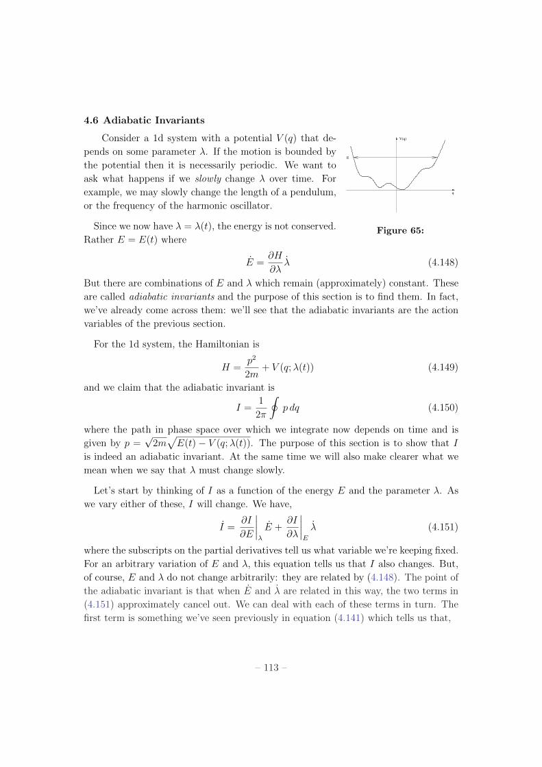
4.6 Adiabatic Invariants
Consider a 1d system with a potential V (q) that de- V(q)
q
E
Figure 65:
pends on some parameter �. If the motion is bounded by
the potential then it is necessarily periodic. We want to
ask what happens if we slowly change � over time. For
example, we may slowly change the length of a pendulum,
or the frequency of the harmonic oscillator.
Since we now have � = �(t), the energy is not conserved.
Rather E = E(t) where
E =@H
@�� (4.148)
But there are combinations of E and � which remain (approximately) constant. These
are called adiabatic invariants and the purpose of this section is to find them. In fact,
we’ve already come across them: we’ll see that the adiabatic invariants are the action
variables of the previous section.
For the 1d system, the Hamiltonian is
H =p2
2m+ V (q;�(t)) (4.149)
and we claim that the adiabatic invariant is
I =1
2⇡
I
p dq (4.150)
where the path in phase space over which we integrate now depends on time and is
given by p =p2mp
E(t)� V (q;�(t)). The purpose of this section is to show that I
is indeed an adiabatic invariant. At the same time we will also make clearer what we
mean when we say that � must change slowly.
Let’s start by thinking of I as a function of the energy E and the parameter �. As
we vary either of these, I will change. We have,
I =@I
@E
�
�
�
�
�
E +@I
@�
�
�
�
�
E
� (4.151)
where the subscripts on the partial derivatives tell us what variable we’re keeping fixed.
For an arbitrary variation of E and �, this equation tells us that I also changes. But,
of course, E and � do not change arbitrarily: they are related by (4.148). The point of
the adiabatic invariant is that when E and � are related in this way, the two terms in
(4.151) approximately cancel out. We can deal with each of these terms in turn. The
first term is something we’ve seen previously in equation (4.141) which tells us that,
– 113 –
q
p
λ
λ
1
2
Figure 66:
@I
@E
�
�
�
�
�
=1
!(�)=
T (�)
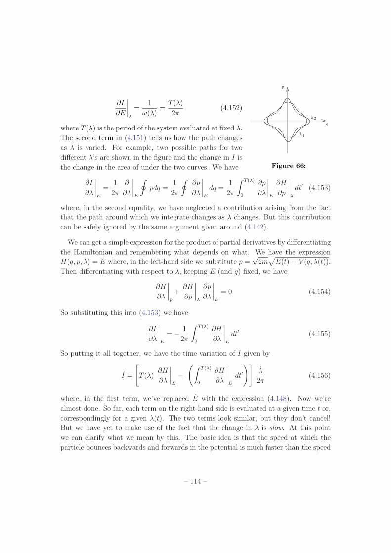
2⇡(4.152)
where T (�) is the period of the system evaluated at fixed �.
The second term in (4.151) tells us how the path changes
as � is varied. For example, two possible paths for two
di↵erent �’s are shown in the figure and the change in I is
the change in the area of under the two curves. We have
@I
@�
�
�
�
�
E
=1
2⇡
@
@�
�
�
�
�
E
I
pdq =1
2⇡
I
@p
@�
�
�
�
�
E
dq =1
2⇡
Z
T (�)
0
@p
@�
�
�
�
�
E
@H
@p
�
�
�
�
�
dt0 (4.153)
where, in the second equality, we have neglected a contribution arising from the fact
that the path around which we integrate changes as � changes. But this contribution
can be safely ignored by the same argument given around (4.142).
We can get a simple expression for the product of partial derivatives by di↵erentiating
the Hamiltonian and remembering what depends on what. We have the expression
H(q, p,�) = E where, in the left-hand side we substitute p =p2mp
E(t)� V (q;�(t)).
Then di↵erentiating with respect to �, keeping E (and q) fixed, we have
@H
@�
�
�
�
�
p
+@H
@p
�
�
�
�
�
@p
@�
�
�
�
�
E
= 0 (4.154)
So substituting this into (4.153) we have
@I
@�
�
�
�
�
E
= � 1
2⇡
Z
T (�)
0
@H
@�
�
�
�
�
E
dt0 (4.155)
So putting it all together, we have the time variation of I given by
I =
"
T (�)@H
@�
�
�
�
�
E
�
Z
T (�)
0
@H
@�
�
�
�
�
E
dt0!#
�
2⇡(4.156)
where, in the first term, we’ve replaced E with the expression (4.148). Now we’re
almost done. So far, each term on the right-hand side is evaluated at a given time t or,
correspondingly for a given �(t). The two terms look similar, but they don’t cancel!
But we have yet to make use of the fact that the change in � is slow. At this point
we can clarify what we mean by this. The basic idea is that the speed at which the
particle bounces backwards and forwards in the potential is much faster than the speed
– 114 –
at which � changes. This means that the particle has performed many periods before
it notices any appreciable change in the potential. This means that if we compute
averaged quantities over a single period,
hA(�)i = 1
T
Z
T
0
A(t,�) dt (4.157)
then inside the integral we may treat � as if it is e↵ectively constant. We now consider
the time averaged motion hIi. Since � can be taken to be constant over a single period,
the two terms in (4.156) do now cancel. We have
hIi = 0 (4.158)
This is the statement that I is an adiabatic invariant: for small changes in �, the
averaged value of I remains constant6.
The adiabatic invariants played an important role in the early history of quantum
mechanics. You might recognise the quantity I as the object which takes integer values
according to the old 1915 Bohr-Sommerfeld quantisation condition
1
2⇡
I
p dq = n~ n 2 Z (4.159)
The idea that adiabatic invariants and quantum mechanics are related actually predates
the Bohr-Somerfeld quantisation rule. In the 1911 Solvay conference Einstein answered
a question of Lorentz: if the energy is quantised as E = ~n! where n 2 Z then what
happens if ! is changed slowly? Lorentz’ worry was that integers cannot change slowly
– only by integer amounts. Einstein’s answer was not to worry: E/! remains constant.
These days the idea of adiabatic invariants in quantum theory enters into the discussion
of quantum computers.
An Example: The Simple Harmonic Oscillator
We saw in section 4.5 that for the simple harmonic oscillator we have I = E/!. So
if we change ! slowly, then the ratio E/! remains constant. This was Einstein’s 1911
point. In fact, for the SHO it turns out that there is an exact invariant that remains
constant no matter how quickly you change ! and which, in the limit of slow change,
goes over to I. This exact invariant is
J =1
2
q2
g(t)2+ (g(t)q � qg(t))2
�
(4.160)
6The proof given above is intuitive, but begins to creak at the seams when pushed. A nice descrip-
tion of these issues, together with a more sophisticated proof using generating functions for canonical
transformations is given in in the paper “The Adiabatic Invariance of the Action Variable in Classical
Dynamics” by C.G.Wells and S.T.Siklos which can be found at http://arxiv.org/abs/physics/0610084.
– 115 –
where g(t) is a function satisfying the di↵erential equation
g + !2(t)g � 1
g3= 0 (4.161)
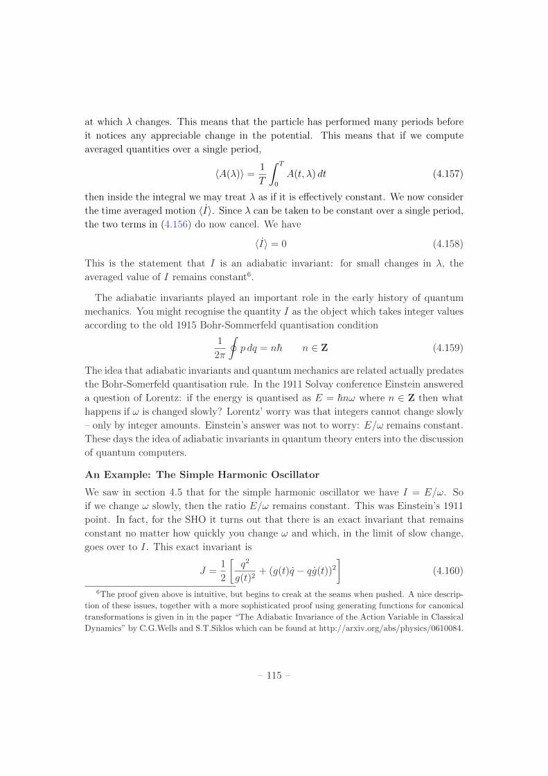
4.6.1 Adiabatic Invariants and Liouville’s Theorem
There’s a way to think of adiabatic invariants using Li-
q
p
Figure 67:
ouville’s theorem. Consider first a series of systems, all
described by a Hamiltonian with fixed parameter �. We
set o↵ each system with the same energy E or, equiva-
lently, the same action I, but we start them with slightly
di↵erent phases ✓. This means that their dynamics is de-
scribed by a series of dots, all chasing each other around a
fixed curve as shown in the figure. Now let’s think about
how this train of dots evolves under the Hamiltonian with
time dependent �(t). Recall that Liouville’s theorem states
that the area of phase space is invariant under any Hamiltonian evolution. This holds
whether or not @H/@t = 0, so is still valid for the time dependent Hamiltonian with
�(t). One might be tempted to say that we’re done since all the words sound right:
Liouville’s theorem implies that the area is conserved which is also the statement that
our adiabatic invariant I doesn’t change with time. But this is a little too fast! Liou-
ville’s theorem says the area of a distribution of particles in phase space is conserved,
not the area enclosed by a perimeter ring of particles. Indeed, Liouville’s theorem holds
for any variation �(t), not just for adiabatic variations. For a fast change of �(t), there
is nothing to ensure that the particles that had the same initial energy, but di↵erent
phases, would have the same final energy and we lose the interpretation of a ring of
dots in phase space enclosing some area.
The missing ingredient is the “adiabatic principle”. In this context it states that for
a suitably slow change of the parameter �, all the systems in the same orbit, with the
same energy, are a↵ected in the same manner. If this holds, after some time the dots
in phase space will still be chasing each other around another curve of constant energy
E 0. We can now think of a distribution of particles filling the area I inside the curve.
As � varies slowly, the area doesn’t change and the outer particles remain the outer
particles, all with the same energy. Under these circumstances, Liouville’s theorem
implies the adiabatic invariant I is constant in time.
4.6.2 An Application: A Particle in a Magnetic Field
We saw in Section 4.1 that a particle in a constant magnetic field B = (0, 0, B) makes
circles with Larmor frequency ! = eB/mc and a radius R, which depends on the energy
– 116 –
of the particle. But what happens if B is slowly varying over space? i.e. B = B(x, y),
but with
@i
B ⌧ R (4.162)
so that the field is roughly constant over one orbit.
In this example, there is no explicit time dependence of the Hamiltonian so we know
that the Hamiltonian itself is an exact constant of motion. For a particle in a constant
magnetic field we can calculate H of an orbit by substituting the solutions (4.32) into
the Hamiltonian (4.28). We find
H =1
2m!2R2 =
e2R2B2
2mc2(4.163)
This quantity is conserved. But what happens to the particle? Does it drift to regions
with larger magnetic field B, keeping H constant by reducing the radius of the orbit?
Or to regions with smaller B with larger orbits?
We can answer this by means of the adiabatic invariant. We can use this because the
motion of the particle is periodic in space so the particle sees a magnetic field which
varies slowly over time. The adiabatic invariant is
I =1
2⇡
I
p dq (4.164)
which is now to be thought of as a path integral along the orbit of the electron. We
evaluate this on the solution for the uniform magnetic field (4.32)
I =1
2⇡
Z
T
0
(px
x+ py
y) dt
=1
2⇡
Z
T
0
�
bR! cos!t+m!2R2 sin2 !t�
dt
=m!R2
2⇡
Z
2⇡
0
sin2 ✓ d✓ (4.165)
Setting ! = eB/mc, we see that the adiabatic invariant I is proportional to (e/c)BR2.
Since the electric charge e and the speed of light c are not things we can change, we find
that BR2 is constant over many orbits. But as H ⇠ B2R2 is also conserved, both the
magnetic field B seen by the particle and the radius of the orbit R must be individually
conserved. This means the particle can’t move into regions of higher or lower magnetic
fields: it must move along constant field lines7.7For results that go beyond the adiabatic approximations, see the paper by the man: E. Witten
“A Slowly Moving Particle in a Two-Dimensional Magnetic Field”, Annals of Physics 120 72 (1979).
– 117 –
Finally, there’s a simple physical way to see that the particle indeed drifts along lines
of constant magnetic field. As the particle makes its little Larmor circles, it feels a
slightly stronger force when it’s, say, at the top of its orbit where the field is slightly
larger, compared to when its at the bottom. This net force tends to push the particle
to regions of weaker or stronger magnetic field. But we’ve seen through the use of
adiabatic invariants that this isn’t possible. The slow drift of the particle acts such
that it compensates for this small force, keeping the particle on constant field lines.
There’s a slight variant of the above set-up which allows you to trap charged particles
using magnetic fields. Consider the particle making its little Larmor circles in the (x, y)
plane, but also moving in the z direction and take a magnetic field that’s constant in
the (x, y)-plane, but ever increasing in the z-direction. The energy of the particle is
given by,
H =1
2mz2 +
e2R2B2
2mc2=
1
2mz2 +
IemB
mc(4.166)
Both H > 0 and I > 0 are constant in time. This ensures that there exists a value of
the magnetic field B > 0 at which we necessarily have z = 0 and the particle can go
no further. At this stage it turns round and goes back again. By creating a magnetic
field that increases at two ends, charged particles can be made to bounce back and
forth in the z direction, while executing their little circles in the (x, y)-plane. It is this
mechanism that traps charged particles in magnetic loops emitted from the sun and is
ultimately responsible for solar flares.
4.6.3 Hannay’s Angle
Consider a particle bouncing around, with periodic motion, in an arbitrary potential.
There are many parameters �a
describing the shape of the potential. As we slowly vary
the �a
the path in phase space changes although, as we have seen, the area enclosed
by the path remains the same. After some time tlong
(which, by the assumption of
adiabiticity, is much longer than the period T of a single orbit) we return to the original
parameters so that �a
(tlong
) = �a
(0). The question we want to ask is: how has the
phase angle ✓ changed?
For any fixed �a
, the velocity of the angle variable is ✓ = @H/@I = !(I,�a
). As
we slowly vary the parameters, the particle is spinning around its phase space orbits.
When we return we therefore expect that the phase has been shifted byR
!dt. Which
is true. But it turns out that there is another, more subtle, contribution to the phase
shift as well. We’ll now see where this comes from.
– 118 –
As the parameters change, we can write the change in the angle ✓ as
✓ =@H
@I+
@✓
@�a
�a
(4.167)
Which looks simple enough. But there’s a problem. The second term is not well defined.
For each set of parameters �a
we have di↵erent action angle variables I(�a
) and ✓(�a
).
But there’s nothing that stops choosing a di↵erent origin ✓ = 0 for each choice of the
parameters. In other words, we could always redefine
✓(�a
) ! ✓(�a
) + �(�a
) (4.168)
where we shift by a di↵erent constant � for each �a
. What this means is that it doesn’t
really make any sense to compare the angle variable for di↵erent parameters �a
. This
makes the second term — which tells us how the angle variable changes as we change
the parameters — ambiguous. One might think this means that we can just ignore it.
Or, more precisely, we could choose the shifts � so that the angle variables are defined
in such a way that the second term vanishes. But it turns out that this isn’t possible.
Let’s see why. The point is that it does make sense to compare the angle variable for
the same parameters �a
. After such a time tlong
, we have
✓(tlong
) = ✓(0) +
Z
tlong
0
! dt+�✓ (4.169)
The termR
!dt is the dynamic term that we anticipated above, arising from the fact
that ✓ is continually making orbits around the curve in phase space. It depends on the
time tlong
that we took to make the change. The other term that we call �✓ is more
interesting. From (4.167) it is given by
�✓ =
Z
tlong
0
⌧
@✓
@�a
�
�i
dt =
I
C
⌧
@✓
@�a
�
d�a
(4.170)
where we’ve used the fact that the change in �a
is adiabatic to replace the integrand
with its average over one period of the orbit. The final expression above means an
integration over the curve C that the system traces in parameter space. We see that
�✓ is independent of the time tlong
taken to make the change. However, it does depend
on the path that we took through the space of all possible potentials. It is known as
the ”Hannay angle”. Note that the Hannay angle is invariant under the ambiguity
(4.169) even though the quantity @✓/@�a
that appears in the integrand isn’t. This
idea of integrating quantities around loops is an example of ”holonomy”, an important
concept in modern physics.
– 119 –
Rather surprisingly, the Hannay angle was first discovered only in 1984. The history
is interesting. First Berry discovered a similar phase for the wavefunction in quantum
mechanics (now known as the Berry phase). Many physicists were shocked that such
a simple and profound idea as Berry’s phase had lain hidden in the formulation of
quantum mechanics for 50 years and it set o↵ a flurry of theoretical and experimental
research. Soon after this, Hannay showed that an analogous phase had lain undis-
covered in classical mechanics for 150 years! Although, in certain examples in celestial
mechanics, the phase �✓ had been correctly calculated, the general theory lying behind
it had not been appreciated. We now describe this theory.
The first step is to use a higher dimensional version of Stokes’ theorem to express
the contour integral (4.170) as a surface integral
�✓ =
Z
S
✓
@
@�a
⌧
@✓
@�b
�
� @
@�b
⌧
@✓
@�a
�◆
dAab
(4.171)
where S is a surface in parameter space bounded by the curve C and dAab
is the in-
finitesimal surface element.
Claim: The Hannay angle can be written as
�✓ =d
dI
Z
S
Wab
dAab
(4.172)
where the anti-symmetric matrix Wab
(known mathematically as a 2-form) is given by
Wab
=
⌧
@✓
@�a
@I
@�b
� @✓
@�b
@I
@�a
�
(4.173)
Proof: To start with let’s think about the averaging procedure a little more. In
equation (4.157) we wrote hAi as a time average, integrating over a single period. We
could equally as well write it as an angle average,
hAi =I
A(I, ✓) d✓ =
Z
A(q0, p0) �(I 0 � I)dq0dp0
2⇡(4.174)
where in the second equality we integrate over all of phase space and insert the delta
function �(I 0 � I) to restrict the integral to the orbit over the curve with action I. It’s
this latter formula that we’ll use. This allows us to write,
@
@�a
⌧
@✓
@�b
�
� @
@�b
⌧
@✓
@�a
�
=
@
@�a
Z
@✓
@�b
� @
@�b
Z
@✓
@�a
�
�(I 0 � I)dq0dp0
2⇡
– 120 –
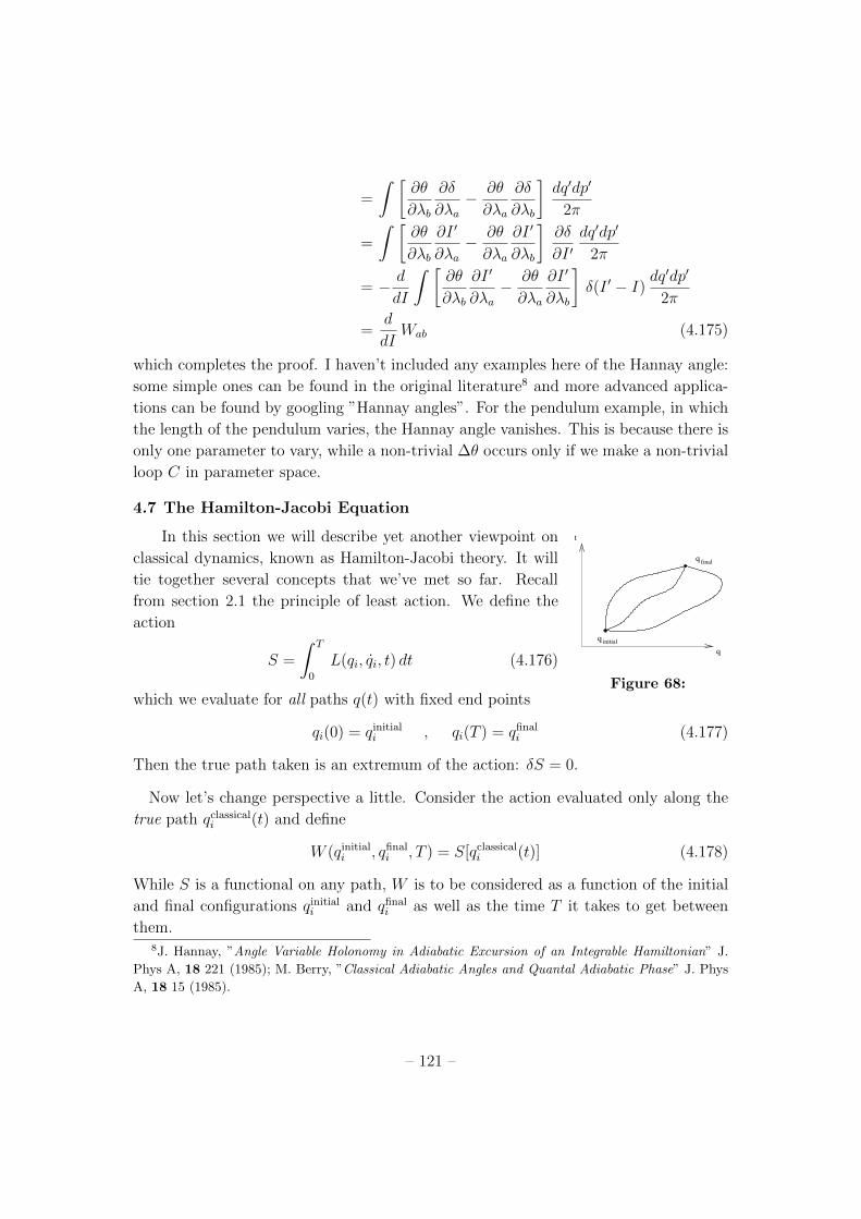
=
Z
@✓
@�b
@�
@�a
� @✓
@�a
@�
@�b
�
dq0dp0
2⇡
=
Z
@✓
@�b
@I 0
@�a
� @✓
@�a
@I 0
@�b
�
@�
@I 0dq0dp0
2⇡
= � d
dI
Z
@✓
@�b
@I 0
@�a
� @✓
@�a
@I 0
@�b
�
�(I 0 � I)dq0dp0
2⇡
=d
dIW
ab
(4.175)
which completes the proof. I haven’t included any examples here of the Hannay angle:
some simple ones can be found in the original literature8 and more advanced applica-
tions can be found by googling ”Hannay angles”. For the pendulum example, in which
the length of the pendulum varies, the Hannay angle vanishes. This is because there is
only one parameter to vary, while a non-trivial �✓ occurs only if we make a non-trivial
loop C in parameter space.
4.7 The Hamilton-Jacobi Equation
In this section we will describe yet another viewpoint on t
initial
final
q
q
q
Figure 68:
classical dynamics, known as Hamilton-Jacobi theory. It will
tie together several concepts that we’ve met so far. Recall
from section 2.1 the principle of least action. We define the
action
S =
Z
T
0
L(qi
, qi
, t) dt (4.176)
which we evaluate for all paths q(t) with fixed end points
qi
(0) = qinitiali
, qi
(T ) = qfinali
(4.177)
Then the true path taken is an extremum of the action: �S = 0.
Now let’s change perspective a little. Consider the action evaluated only along the
true path qclassicali
(t) and define
W (qinitiali
, qfinali
, T ) = S[qclassicali
(t)] (4.178)
While S is a functional on any path, W is to be considered as a function of the initial
and final configurations qinitiali
and qfinali
as well as the time T it takes to get between
them.8J. Hannay, ”Angle Variable Holonomy in Adiabatic Excursion of an Integrable Hamiltonian” J.
Phys A, 18 221 (1985); M. Berry, ”Classical Adiabatic Angles and Quantal Adiabatic Phase” J. Phys
A, 18 15 (1985).
– 121 –
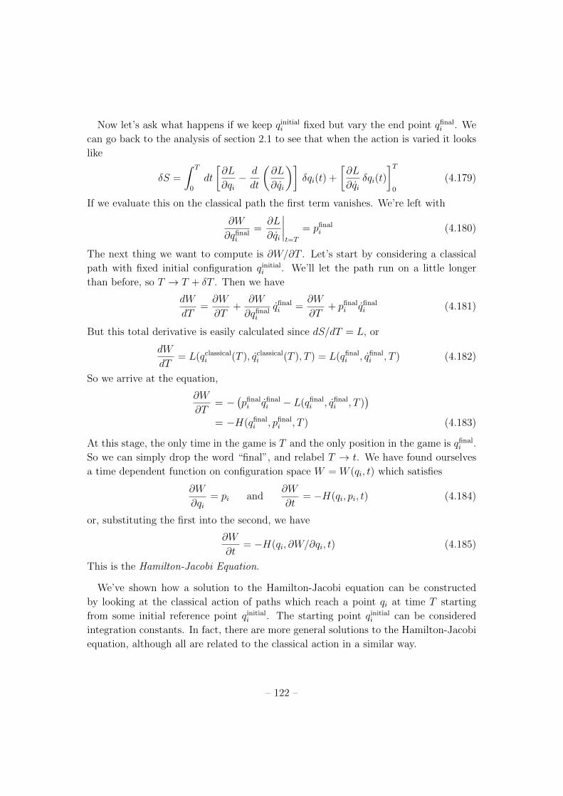
Now let’s ask what happens if we keep qinitiali
fixed but vary the end point qfinali
. We
can go back to the analysis of section 2.1 to see that when the action is varied it looks
like
�S =
Z
T
0
dt
@L
@qi
� d
dt
✓
@L
@qi
◆�
�qi
(t) +
@L
@qi
�qi
(t)
�
T
0
(4.179)
If we evaluate this on the classical path the first term vanishes. We’re left with
@W
@qfinali
=@L
@qi
�
�
�
�
t=T
= pfinali
(4.180)
The next thing we want to compute is @W/@T . Let’s start by considering a classical
path with fixed initial configuration qinitiali
. We’ll let the path run on a little longer
than before, so T ! T + �T . Then we have
dW
dT=@W
@T+
@W
@qfinali
qfinali
=@W
@T+ pfinal
i
qfinali
(4.181)
But this total derivative is easily calculated since dS/dT = L, or
dW
dT= L(qclassical
i
(T ), qclassicali
(T ), T ) = L(qfinali
, qfinali
, T ) (4.182)
So we arrive at the equation,
@W
@T= � �pfinal
i
qfinali
� L(qfinali
, qfinali
, T )�
= �H(qfinali
, pfinali
, T ) (4.183)
At this stage, the only time in the game is T and the only position in the game is qfinali
.
So we can simply drop the word “final”, and relabel T ! t. We have found ourselves
a time dependent function on configuration space W = W (qi
, t) which satisfies
@W
@qi
= pi
and@W
@t= �H(q
i
, pi
, t) (4.184)
or, substituting the first into the second, we have
@W
@t= �H(q
i
, @W/@qi
, t) (4.185)
This is the Hamilton-Jacobi Equation.
We’ve shown how a solution to the Hamilton-Jacobi equation can be constructed
by looking at the classical action of paths which reach a point qi
at time T starting
from some initial reference point qinitiali
. The starting point qinitiali
can be considered
integration constants. In fact, there are more general solutions to the Hamilton-Jacobi
equation, although all are related to the classical action in a similar way.
– 122 –
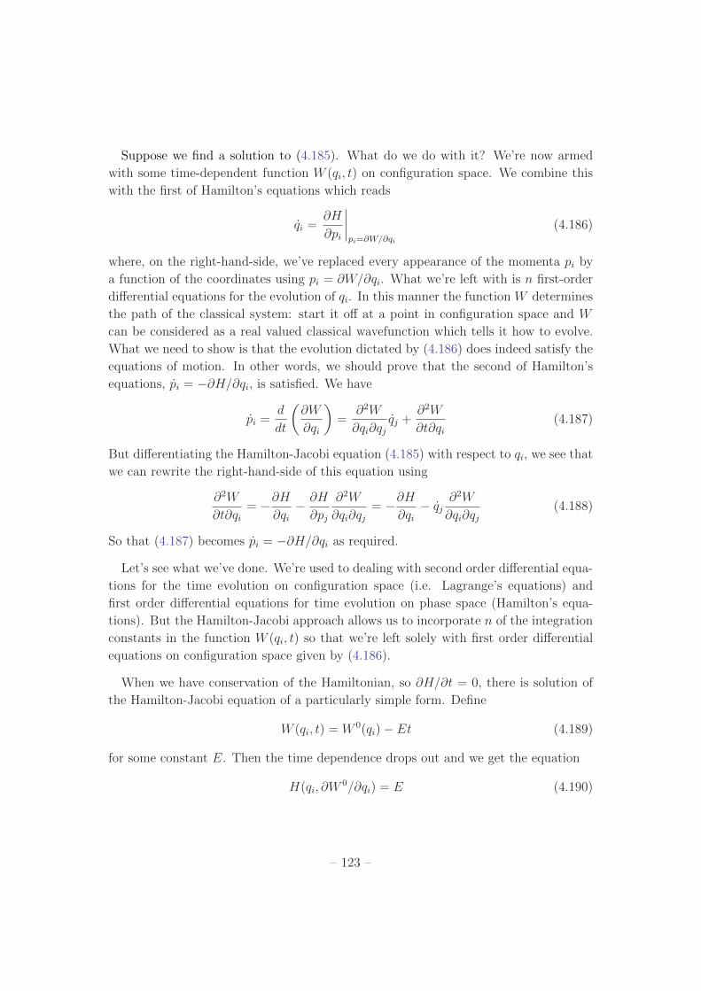
Suppose we find a solution to (4.185). What do we do with it? We’re now armed
with some time-dependent function W (qi
, t) on configuration space. We combine this
with the first of Hamilton’s equations which reads
qi
=@H
@pi
�
�
�
�
pi=@W/@qi
(4.186)
where, on the right-hand-side, we’ve replaced every appearance of the momenta pi
by
a function of the coordinates using pi
= @W/@qi
. What we’re left with is n first-order
di↵erential equations for the evolution of qi
. In this manner the function W determines
the path of the classical system: start it o↵ at a point in configuration space and W
can be considered as a real valued classical wavefunction which tells it how to evolve.
What we need to show is that the evolution dictated by (4.186) does indeed satisfy the
equations of motion. In other words, we should prove that the second of Hamilton’s
equations, pi
= �@H/@qi
, is satisfied. We have
pi
=d
dt
✓
@W
@qi
◆
=@2W
@qi
@qj
qj
+@2W
@t@qi
(4.187)
But di↵erentiating the Hamilton-Jacobi equation (4.185) with respect to qi
, we see that
we can rewrite the right-hand-side of this equation using
@2W
@t@qi
= �@H@q
i
� @H
@pj
@2W
@qi
@qj
= �@H@q
i
� qj
@2W
@qi
@qj
(4.188)
So that (4.187) becomes pi
= �@H/@qi
as required.
Let’s see what we’ve done. We’re used to dealing with second order di↵erential equa-
tions for the time evolution on configuration space (i.e. Lagrange’s equations) and
first order di↵erential equations for time evolution on phase space (Hamilton’s equa-
tions). But the Hamilton-Jacobi approach allows us to incorporate n of the integration
constants in the function W (qi
, t) so that we’re left solely with first order di↵erential
equations on configuration space given by (4.186).
When we have conservation of the Hamiltonian, so @H/@t = 0, there is solution of
the Hamilton-Jacobi equation of a particularly simple form. Define
W (qi
, t) = W 0(qi
)� Et (4.189)
for some constant E. Then the time dependence drops out and we get the equation
H(qi
, @W 0/@qi
) = E (4.190)
– 123 –
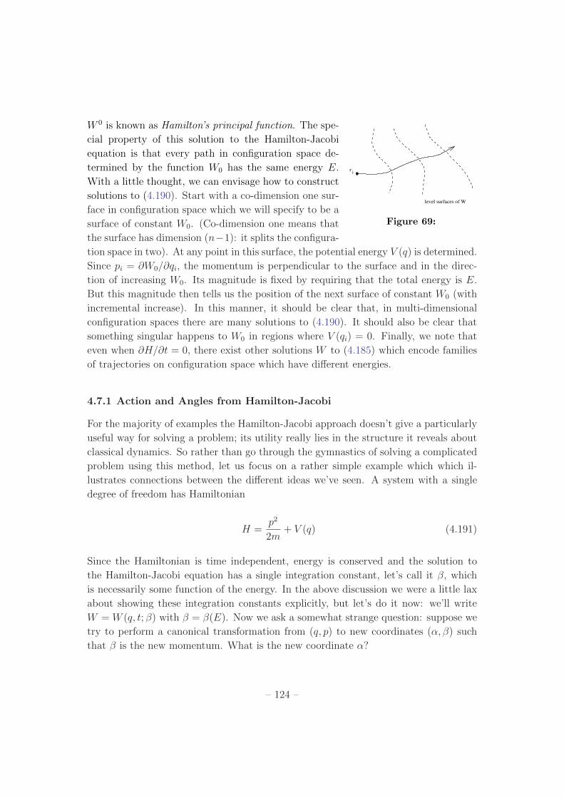
W 0 is known as Hamilton’s principal function. The spe-
ir
level surfaces of W
Figure 69:
cial property of this solution to the Hamilton-Jacobi
equation is that every path in configuration space de-
termined by the function W0
has the same energy E.
With a little thought, we can envisage how to construct
solutions to (4.190). Start with a co-dimension one sur-
face in configuration space which we will specify to be a
surface of constant W0
. (Co-dimension one means that
the surface has dimension (n�1): it splits the configura-
tion space in two). At any point in this surface, the potential energy V (q) is determined.
Since pi
= @W0
/@qi
, the momentum is perpendicular to the surface and in the direc-
tion of increasing W0
. Its magnitude is fixed by requiring that the total energy is E.
But this magnitude then tells us the position of the next surface of constant W0
(with
incremental increase). In this manner, it should be clear that, in multi-dimensional
configuration spaces there are many solutions to (4.190). It should also be clear that
something singular happens to W0
in regions where V (qi
) = 0. Finally, we note that
even when @H/@t = 0, there exist other solutions W to (4.185) which encode families
of trajectories on configuration space which have di↵erent energies.
4.7.1 Action and Angles from Hamilton-Jacobi
For the majority of examples the Hamilton-Jacobi approach doesn’t give a particularly
useful way for solving a problem; its utility really lies in the structure it reveals about
classical dynamics. So rather than go through the gymnastics of solving a complicated
problem using this method, let us focus on a rather simple example which which il-
lustrates connections between the di↵erent ideas we’ve seen. A system with a single
degree of freedom has Hamiltonian
H =p2
2m+ V (q) (4.191)
Since the Hamiltonian is time independent, energy is conserved and the solution to
the Hamilton-Jacobi equation has a single integration constant, let’s call it �, which
is necessarily some function of the energy. In the above discussion we were a little lax
about showing these integration constants explicitly, but let’s do it now: we’ll write
W = W (q, t; �) with � = �(E). Now we ask a somewhat strange question: suppose we
try to perform a canonical transformation from (q, p) to new coordinates (↵, �) such
that � is the new momentum. What is the new coordinate ↵?
– 124 –
Since we wish the change of coordinates to be canonical, we must be able to write
q = q(↵, �) and p = p(↵, �) such that
{q, p}(↵,�)
⌘ @q
@↵
@p
@�� @q
@�
@p
@↵= 1 (4.192)
Using p = @W/@q and remembering what all depends on what all (W = W (q, �) and
q = q(↵, �) and p = p(↵, �)) we can write this as,
{q, p}(↵,�)
=@q
@↵
✓
@2W
@�@q+@2W
@q2@q
@�
◆
� @q
@�
@2W
@q2@q
@↵=@q
@↵
@
@q
✓
@W
@�
◆
(4.193)
and we find that the transformation is canonical if we take ↵ = @W/@�. Note the nice
symmetry here: we have a solution W (q, t; �) to the Hamilton Jacobi equation and we
can think in terms of canonical coordinates (q, p) or alternatively (↵, �) where
p =@W
@q, ↵ =
@W
@�(4.194)
The function W is an example of a generating function of the second kind (4.120).
So what to do with this? Let’s look at some examples. Take � = E, so that our new
momentum variable is the energy itself. What is the canonical coordinate? If we write
W (q, t;E) = W0
(q, E)� Et then the coordinate canonically dual to E is
↵ =@W
0
@E(q, E)� t (4.195)
Taking the time dependence over the left-hand-side, we see that ↵ has the interpretation
of �t0
, the initial starting time. This tells us that we may parameterise every trajectory
in a one-dimensional system in terms of the energy and starting time of the path, and
that these are canonical variables. Again we see the dual relationship between energy
and time. Note that both E and t0
are independent of time; we’ve found canonical
variables for which neither the coordinate nor the momentum vary along the path.
As another example consider the case of � = I, our action variable of Section 4.5.
What is the canonical coordinate ↵ in this case? We expect that it will be related to
the angle variable ✓. To see this, we use the fact that W is the classical action to write
W0
=
Z
Ldt+ Et =
Z
(L+H)dt =
Z
qp dt =
Z
p dq (4.196)
So we have that
↵ =@W
@�=
d
dI
Z
p dq � dE
dIt = ✓ � !t (4.197)
– 125 –
where we’ve used our expression (4.144) for the angle variable, as well as the equation
(4.141) for the frequency of motion !. So we see that ↵ is not quite equal to ✓,
but is shifted by a term linear in time. In fact this means that ↵ itself does not
change in time. Once again, we’ve arrived at a way to parameterise the orbits of
motion by canonical variables which do not themselves change with time. In fact, in
most presentations, this is the starting motivation for the Hamilton-Jacobi approach
to classical dynamics and, even for higher dimensional systems, the function W can
be thought of as a way to generate new, time independent, canonical variables. More
discussion on the relationship between canonical transformations, angle-action variables
and the Hamilton-Jacobi formulation can be found in the book by Hand and Finch, or
deep within Goldstein.
4.8 Quantum Mechanics
One of the primary reasons for studying the rather formal aspects of classical mechanics
discussed in this course is to make contact with quantum mechanics. For this reason,
in this last section of the course we will illustrate the connection between the classical
and quantum world and point out a few analogies that might just make the quantum
behaviour look a little less weird. (Just a little less: after all, it really is weird!)
In classical mechanics the state of a system is described by a point (qi
, pi
) in phase
space. In quantum mechanics the state is described by a very di↵erent object: a
complex valued wavefunction (q) over the configuration space. The observables are
operators on the space of wavefunctions. The standard representations of the position
operator qi
and momentum operator pi
are
qi
(q) = qi
(q)
pi
(q) = i~@ @q
i
(4.198)
which leads to the well known Heisenberg commutation relations
[pi
, pj
] = 0
[qi
, qj
] = 0 (4.199)
[qi
, pj
] = i~ �ij
Of course, we’ve already seen something very familiar in section 4.3 on Poisson brackets
as summarised in equation (4.61). Although the bilinear, antisymmetric operators
[ , ] and { , } act on very di↵erent spaces, they carry the same algebraic structure.
Heuristically the relations (4.61) and (4.199) both represent the mathematical fact
– 126 –
that momentum pi
generates infinitesimal translations of qi
: in classical mechanics we
saw this in when we studied infinitesimal canonical transformations in section 4.4.1; in
quantum mechanics it follows from the representation (4.198) and Taylor’s expansion.
In general the map between a classical system and a quantum system goes via the
Poisson brackets and was formulated by Dirac:
{ , }classical
$ � i
~ [ , ]quantum
(4.200)
This prescription for going between the classical and quantum theories is known as
canonical quantisation. It also gives rise to the quantum equations of motion. In the
Poisson bracket language, we have seen that the classical equation of motion for an
arbitrary function f(q, p) is
f = {f,H} �! i~ ˙f = [f , H] (4.201)
which is the equation of motion in the Heisenberg picture, in which the time dependence
is assigned to the operator rather than the state.
While a great physicist, Dirac was never much of a storyteller. It shows in the
following anecdote recounting his graduate student days:
“I went back to Cambridge at the beginning of October 1925, and resumed
my previous style of life, intense thinking about these problems during the
week and relaxing on Sunday, going for a long walk in the country alone.
The main purpose of these long walks was to have a rest so that I would
start refreshed on the following Monday.
It was during one of the Sunday walks in October 1925, when I was think-
ing about this (uv � vu), in spite of my intention to relax, that I thought
about Poisson brackets. I remembered something which I had read up previ-
ously, and from what I could remember, there seemed to be a close similarity
between a Poisson bracket of two quantities and the commutator. The idea
came in a flash, I suppose, and provided of course some excitement, and
then came the reaction “No, this is probably wrong”.
I did not remember very well the precise formula for a Poisson bracket,
and only had some vague recollections. But there were exciting possibilities
there, and I thought that I might be getting to some big idea. It was really
a very disturbing situation, and it became imperative for me to brush up on
– 127 –
my knowledge of Poisson brackets. Of course, I could not do that when I
was right out in the countryside. I just had to hurry home and see what I
could find about Poisson brackets.
I looked through my lecture notes, the notes that I had taken at various
lectures, and there was no reference there anywhere to Poisson brackets.
The textbooks which I had at home were all too elementary to mention them.
There was nothing I could do, because it was Sunday evening then and the
libraries were all closed. I just had to wait impatiently through that night
without knowing whether this idea was really any good or not, but I still
think that my confidence gradually grew during the course of the night.
The next morning I hurried along to one of the libraries as soon as it
was open, and then I looked up Poisson brackets in Whitackers Analytical
Dynamics, and I found that they were just what I needed.”
4.8.1 Hamilton, Jacobi, Schrodinger and Feynman
While the Poisson bracket structure of quantum mechanics dovetails nicely with Heisen-
berg’s approach, the Hamilton-Jacobi equation is closely tied to Schrodinger’s wave
equation. Let’s first recall what Schrodinger’s equation looks like for a one-dimensional
system with a Hamiltonian operator H = p2/2m+ V (q) acting on wavefunctions (q),
i~ @ @t
= H = � ~22m
@2
@q2+ V (q) (4.202)
where we have used the representation (4.198) for the position and momentum opera-
tors. To see the relationship of this equation to classical dynamics we decompose the
wavefunction into the modulus and phase,
(q, t) = R(q, t) eiW (q,t)/~ (4.203)
where R and W are both real functions. We know that R is related to the probability
P for finding a particle at position q at time t: P (q, t) = | (q, t)|2 = R(q, t)2. But what
is the interpretation of the phase W? Let’s substitute this decomposition of into the
Schrodinger equation to find
i~
@R
@t+
iR
~@W
@t
�
= � ~22m
"
@2R
@q2+
2i
~@R
@q
@W
@q� R
~2
✓
@W
@q
◆
2
+iR
~@2W
@q2
#
+ V R
– 128 –
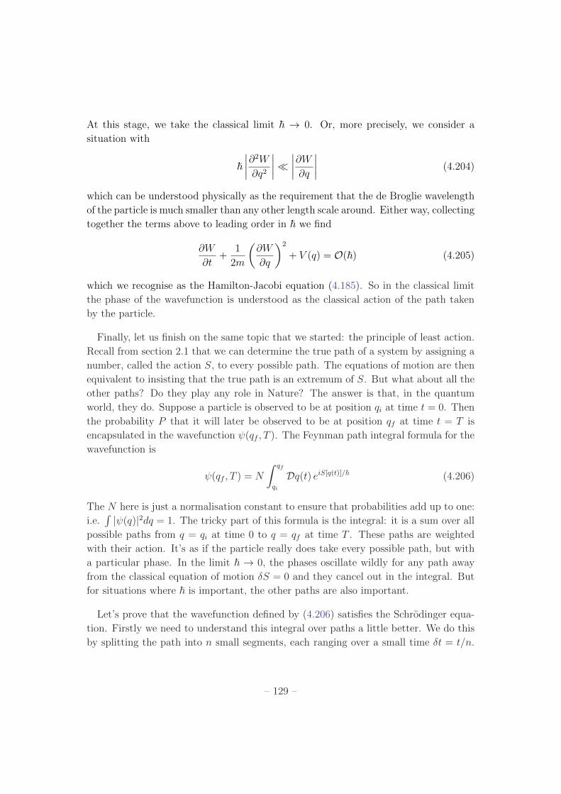
At this stage, we take the classical limit ~ ! 0. Or, more precisely, we consider a
situation with
~�
�
�
�
@2W
@q2
�
�
�
�
⌧�
�
�
�
@W
@q
�
�
�
�
(4.204)
which can be understood physically as the requirement that the de Broglie wavelength
of the particle is much smaller than any other length scale around. Either way, collecting
together the terms above to leading order in ~ we find
@W
@t+
1
2m
✓
@W
@q
◆
2
+ V (q) = O(~) (4.205)
which we recognise as the Hamilton-Jacobi equation (4.185). So in the classical limit
the phase of the wavefunction is understood as the classical action of the path taken
by the particle.
Finally, let us finish on the same topic that we started: the principle of least action.
Recall from section 2.1 that we can determine the true path of a system by assigning a
number, called the action S, to every possible path. The equations of motion are then
equivalent to insisting that the true path is an extremum of S. But what about all the
other paths? Do they play any role in Nature? The answer is that, in the quantum
world, they do. Suppose a particle is observed to be at position qi
at time t = 0. Then
the probability P that it will later be observed to be at position qf
at time t = T is
encapsulated in the wavefunction (qf
, T ). The Feynman path integral formula for the
wavefunction is
(qf
, T ) = N
Z
qf
qi
Dq(t) eiS[q(t)]/~ (4.206)
The N here is just a normalisation constant to ensure that probabilities add up to one:
i.e.R | (q)|2dq = 1. The tricky part of this formula is the integral: it is a sum over all
possible paths from q = qi
at time 0 to q = qf
at time T . These paths are weighted
with their action. It’s as if the particle really does take every possible path, but with
a particular phase. In the limit ~ ! 0, the phases oscillate wildly for any path away
from the classical equation of motion �S = 0 and they cancel out in the integral. But
for situations where ~ is important, the other paths are also important.
Let’s prove that the wavefunction defined by (4.206) satisfies the Schrodinger equa-
tion. Firstly we need to understand this integral over paths a little better. We do this
by splitting the path into n small segments, each ranging over a small time �t = t/n.
– 129 –
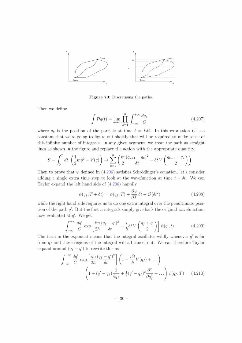
t
initial
final
q
q
q
tδ
t
initial
final
q
q
q
Figure 70: Discretising the paths.
Then we defineZ
Dq(t) = limn!1
n
Y
k=1
Z
+1
�1
dqk
C(4.207)
where qk
is the position of the particle at time t = k�t. In this expression C is a
constant that we’re going to figure out shortly that will be required to make sense of
this infinite number of integrals. In any given segment, we treat the path as straight
lines as shown in the figure and replace the action with the appropriate quantity,
S =
Z
T
0
dt
✓
1
2mq2 � V (q)
◆
!n
X
k=1
✓
m
2
(qk+1
� qk
)2
�t� �t V
✓
qk+1
+ qk
2
◆◆
Then to prove that defined in (4.206) satisfies Schrodinger’s equation, let’s consider
adding a single extra time step to look at the wavefunction at time t + �t. We can
Taylor expand the left hand side of (4.206) happily
(qf
, T + �t) = (qf
, T ) +@
@T�t+O(�t2) (4.208)
while the right hand side requires us to do one extra integral over the penultimate posi-
tion of the path q0. But the first n integrals simply give back the original wavefunction,
now evaluated at q0. We getZ
+1
�1
dq0
Cexp
im
2~(q
f
� q0)2
�t� i
~�t V✓
qf
+ q0
2
◆�
(q0, t) (4.209)
The term in the exponent means that the integral oscillates wildly whenever q0 is far
from qf
and these regions of the integral will all cancel out. We can therefore Taylor
expand around (qf
� q0) to rewrite this asZ
+1
�1
dq0
Cexp
im
2~(q
f
� q0)2
�t
�✓
1� i�t
~ V (qf
) + . . .
◆
1 + (q0 � qf
)@
@qf
+ 1
2
(q0 � qf
)2@2
@q2f
+ . . .
!
(qf
, T ) (4.210)
– 130 –
At this stage we do the integral over q0. We’ll use the formulae for Gaussian integration
Z
dy e�ay
2=
r
⇡
a,
Z
dy ye�ay
2= 0 ,
Z
dy y2e�ay
2=
1
2a
r
⇡
a(4.211)
Then equating the lefthand side (4.208) with the righthand side (4.210), we have
(qf
, T ) +@
@T�t =
1
C
r
2⇡~�t�im
"
1� i�t
~ V (qf
) +i~�t2m
@2
@q2f
+O(�t2)
#
(qf
, T )
At this stage we see what the constant C has to be to make sense of this whole calcu-
lation: we should take
C =
r
2⇡~�t�im
(4.212)
so that C ! 0 as �t ! 0. Then the terms of order O(�t0) agree. Collecting the terms
of order O(�t), and replacing the time T at the end point with the general time t, we
see that we have
i~@ @t
= � ~22m
@2
@q2f
+ V (qf
) = H (4.213)
and we recover Schrodinger’s equation as promised.
4.8.2 Nambu Brackets
Throughout this section, we’ve seen that several of the structures appearing in quantum
mechanics were anticipated, in some form, within the framework of classical dynamics.
You just need to know where to look. One might wonder whether classical mechanics
also contains other structures which will prove to be important in future discoveries.
Or, alternatively, whether there are ways to extend the framework of classical dynamics
that hints at new ways to formulate the laws of physics. In this section, I’ll briefly
describe such an extension due to Nambu in 1973. I should confess immediately that
there’s no known use for Nambu’s formalism! And it’s not at all clear that one will be
found! But then again, maybe it holds the clue that will prove crucial in the search for
the ideas beyond the known laws of Nature.
We’ve seen that the Hamiltonian framework deals with canonical pairs of coordinates
and momenta (qi
, pi
) with i = 1, . . . , n. Nambu’s idea was to extend this to triplets of
objects (qi
, pi
, ri
) with i = 1, . . . , n. We don’t say what this extra variable ri
is: just
that it is necessary to define the state of a system. This means that the phase space
– 131 –
has dimension 3n. The Nambu bracket, which replaces the Poisson bracket, acts on
three functions f, g and h in phase space,
{f, g, h} =X
i
@f
@qi
@g
@pi
@h
@ri
� @f
@qi
@g
@ri
@h
@pi
+@f
@ri
@g
@qi
@h
@pi
� @f
@ri
@g
@pi
@h
@qi
+@f
@pi
@g
@ri
@h
@qi
� @f
@pi
@h
@qi
@h
@ri
(4.214)
This satisfies similar properties to the Poisson bracket, including linearity and
• Anti-symmetry: {f, g, h} = �{g, f, h} = {g, h, f}.• Leibniz: {fg, h, l} = f{g, h, l}+ {f, h, l}g.• “Jacobi”: {{f, g, h}, l,m}+ {h, {f, g, l},m}+ {h, l, {f, g,m}} = {f, g, {h, l,m}}.
In order to specify time evolution, we need two ”Hamiltonians”. We call them H(q, p, r)
and G(q, p, r). Then any function f over phase space evolves as
df
dt= {f,G,H} (4.215)
In particular, the new version Hamilton’s equations read
qi
=@G
@pi
@H
@ri
� @G
@ri
@H
@pi
pi
=@G
@ri
@H
@qi
� @G
@qi
@H
@ri
(4.216)
ri
=@G
@qi
@H
@pi
� @G
@pi
@H
@qi
where there’s no sum over i on the right-hand side of these equations. By the anti-
symmetry of the Nambu bracket, we learn that both H and G are conserved (as long
as neither have explicit time dependence).
Many of the key features of classical dynamics are retained in Nambu’s formalism.
For example, Liouville’s theorem still holds. (This was Nambu’s original motivation
for suggesting this framework). Similarly, canonical transformations can be defined as
a change of variables qi
! Qi
(q, p, r) and pi
! Pi
(q, p, r) and ri
! Ri
(q, p, r) such that
the Nambu bracket structure is preserved, for example
{Qi
, Pj
, Rk
} =
(
1 if i = j = k
0 otherwise(4.217)
together with similar equations involving other combinations of Q’s, P ’s and R’s.
”Hamilton’s” equations (4.216) are invariant under these canonical transformations.
– 132 –
The Nambu bracket provides a generalisation of classical dynamics. But can we
quantise it? In other words, can we find some operators which reproduce the Nambu
bracket structure (up to a factor of ~ and perhaps an i) in much the same way that the
usual quantum theory ties in with the Poisson bracket? This turns out to be pretty
tricky. In particular, it seems di�cult to keep all three conditions: anti-symmetry,
Leibniz and Jacobi. Perhaps this suggests that the correct mathematical structure has
not yet been uncovered. Perhaps it suggests that the Nambu bracket is just not useful!
Chances are that you won’t ever have any use for the Nambu bracket. But you never
know. Perhaps one day, like Dirac, you’ll return from wandering the fields around
Cambridge and desperately need to recall this concept. But, unlike Dirac, you’ll be
able to find a reference in your lecture notes (the notes you had taken at various
lectures).
– 133 –


![arxiv.org · arXiv:2010.01597v1 [math-ph] 4 Oct 2020 Bundle geometry of the connection space, covariant Hamiltonian formalism, the problem of boundaries in gauge theories, and the](https://img.pdfslide.net/doc/110x75/605116b9c2a8ec234d075bc6/arxivorg-arxiv201001597v1-math-ph-4-oct-2020-bundle-geometry-of-the-connection.jpg)


![2cm [height=0.5cm]logos/pyphs.pdf PyPHS: An open source ... · PyPHS background Main tools Port-Hamiltonian Systems (PHS) formalism 3 Graph theory4 2012!2016 ANR project HaMecMoPSys5](https://img.pdfslide.net/doc/110x75/5facf1142d7f3c00ae085c18/2cm-height05cmlogospyphspdf-pyphs-an-open-source-pyphs-background-main.jpg)