4321

Fast Sublinear Sparse Representation using ShallowTree Matching Pursuit

Ali Ayremlou, Member, IEEE, Thomas Goldstein, Member, IEEE Ashok Veeraraghavan, Member, IEEE andRichard Baraniuk, Fellow, IEEE

Abstract—Sparse approximations using highly over-completedictionaries is a state-of-the-art tool for many imaging applica-tions including denoising, super-resolution, compressive sensing,light-field analysis, and object recognition. Unfortunately, theapplicability of such methods is severely hampered by thecomputational burden of sparse approximation: these algorithmsare linear or super-linear in both the data dimensionality andsize of the dictionary.

We propose a framework for learning the hierarchical struc-ture of over-complete dictionaries that enables fast computationof sparse representations. Our method builds on tree-basedstrategies for nearest neighbor matching, and presents domain-specific enhancements that are highly efficient for the analysis ofimage patches. Contrary to most popular methods for buildingspatial data structures, out methods rely on shallow, balancedtrees with relatively few layers.

We show an extensive array of experiments on several ap-plications such as image denoising/superresolution, compressivevideo/light-field sensing where we practically achieve 100-1000xspeedup (with a less than 1dB loss in accuracy).

I. INTRODUCTION

COMPRESSIVE sensing and sparse approximation usingredundant dictionaries are important tools for a wide

range of imaging applications including image/video denoising[1], [2], [3], superresolution [4], [5], compressive sensingof videos [6], [7], [8], light-fields [9], [10], hyperspectraldata [11], and even inference tasks such as face and objectrecognition [12].

In spite of this widespread adoption in research, theiradoption in commercial and practical systems is still lacking.One of the principal reasons is the computational complexityof the algorithms needed: these algorithms are either linear orsuper-linear in both the data dimensionality and size of thedictionary. Common applications requiring dictionaries withover 105 atoms require computation times that may exceedseveral days.

As an illustrative example, consider the problem of com-pressive video sensing using overcomplete dictionaries [8].In [8], an overcomplete dictionary consisting of 105 videopatches was learned and utilized for compressive sensingusing orthogonal matching pursuit (OMP). Reconstruction fora single video (36 frames) using 105 dictionary atoms takesmore than a day, making these methods impractical for mostapplications and highlighting the need for significantly fasteralgorithms.

A. Motivation and Related WorkAlgorithms for sparse approximation can be broadly classi-

fied into two categories: those based on convex optimization,

A. Ayremlou, T. Goldstein, A. Veeraraghavan and R. Baraniuk are with theDepartment of Electrical and Computer Engineering, Rice University, Hous-ton, TX 77005 USA (e-mail: {a.ayremlou, tag7, vashok, richb}@rice.edu).

Level 1

c1

c4

c3

c2

c6

c5

Level 2

c3

c3

c1

c2

Level 3

c2

c1

c3

Test vector

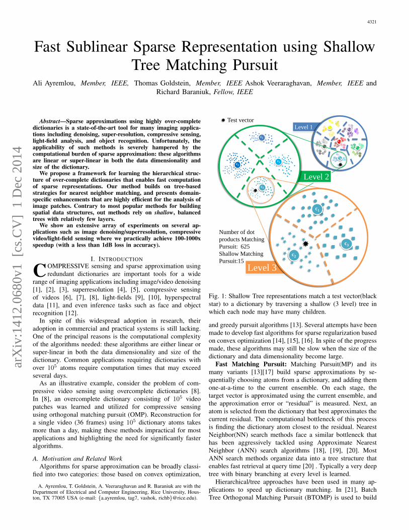
Number of dot

products Matching

Pursuit: 625

Shallow Matching

Pursuit:15

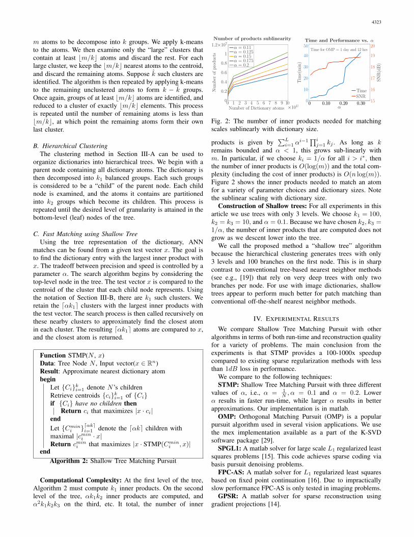
Fig. 1: Shallow Tree representations match a test vector(blackstar) to a dictionary by traversing a shallow (3 level) tree inwhich each node may have many children.

and greedy pursuit algorithms [13]. Several attempts have beenmade to develop fast algorithms for sparse regularization basedon convex optimization [14], [15], [16]. In spite of the progressmade, these algorithms may still be slow when the size of thedictionary and data dimensionality become large.

Fast Matching Pursuit: Matching Pursuit(MP) and itsmany variants [13][17] build sparse approximations by se-quentially choosing atoms from a dictionary, and adding themone-at-a-time to the current ensemble. On each stage, thetarget vector is approximated using the current ensemble, andthe approximation error or “residual” is measured. Next, anatom is selected from the dictionary that best approximates thecurrent residual. The computational bottleneck of this processis finding the dictionary atom closest to the residual. NearestNeighbor(NN) search methods face a similar bottleneck thathas been aggressively tackled using Approximate NearestNeighbor (ANN) search algorithms [18], [19], [20]. MostANN search methods organize data into a tree structure thatenables fast retrieval at query time [20] . Typically a very deeptree with binary branching at every level is learned.

Hierarchical/tree approaches have been used in many ap-plications to speed up dictionary matching. In [21], BatchTree Orthogonal Matching Pursuit (BTOMP) is used to build

arX

iv:1

412.

0680

v1 [

cs.C

V]

1 D

ec 2

014

4322

a feature hierarchy that yields a better classification. Theauthors of [22] construct trees using “kernel descriptors” forthe same application. Hierarchical methods for representingimage patches are studied in [23], [24].The authors of [25]Random prejections for dimensionally reduction are used in[26] to build hierarchical dictionaries. In [27] binary hierar-chical structure and PCA (Principal Component Analysis) arecombined to reduce the complexity of the OMP.

Unfortunately, such a deep tree does not provide a beneficialtrade-off between accuracy and speedup for dictionaries, sincethese atoms tend to be highly coherent. Further, because theyrequire backtracking and branch-and-bound methods, typicalANN techniques such as kd-trees do not provide reliableruntime guarantees.

In contrast, we organize the dictionary using a shallowtree (typically 3 levels) as shown in Figure 1. Our treeconstruction scheme is such that the resulting tree representsa balanced, hierarchical clustering of the atoms. Finally, wedevise a sublinear time search algorithm for identifying thesupport set that provides the user with precise control over thecomputational speedup achieved while retaining high fidelityapproximations.

B. ContributionsWe propose an algorithm for balanced hierarchical cluster-

ing of dictionary atoms. We exploit the clustering to derive asublinear time algorithm for sparse approximation. Our meth-ods has a single parameter α that provides fine-scale control onthe computational speed-up achieved, enabling a natural trade-off between accuracy and computation. We perform extensiveexperiments that span numerous applications where shallowtrees achieve 150-1000x speedup (with a 1dB of less loss inaccuracy) compared to conventional methods.

II. PROBLEM FORMULATIONA. Sparse Approximation using Dictionaries

Our approach to fast dictionary coding uses MatchingPursuit (MP), which is a greedy method for selecting theconstituent dictionary elements that comprise a test vector.MP is a commonly used scheme for this application becausedictionary representations of image patches are extremelysparse. For computing representations involving large numbersof atoms (e.g. for representing entire images rather than justpatches) more complex pursuit algorithms have been proposed[28] that we do not consider here.

Matching Pursuit: MP is a stage-wise scheme that buildsa signal representation one atom at a time. Algorithm 1 isinitialized by declaring the “residual” r to be equal to the testvector x. This residual represents the component of x that hasnot yet been accounted for by the sparse approximation. Ineach iteration of the main loop an atom enters the representa-tion. The atom is selected by computing inner products withall (normalized) columns in D = {di} and selecting the atomwith the largest inner product. The residual is then updated bysubtracting the contribution of the entering dictionary element.

MP Computational Complexity: MP requires the compu-tation of m inner products on the “matching” stage of eachiteration. Since each inner product requires O(n) operationsand there are K stages, the overall complexity is O(mnK).

Data: Normalized Dictionary D ∈ Rn×m, Input vectorx ∈ Rn, Sparsity level K ∈ Z+

Result: Sparse vector s ∈ Rm with x ≈ Dsbegin

r = x/* Main Loop */for k = 1 to K do

i← argmaxi |di · x|si = di · xr ← r − disi

endend

Algorithm 1: Maching Pursuit

Note that this complexity is dominated by m, the number ofatoms in the dictionary. For most imaging applications, D ishighly over-complete. A typical image denoising method mayoperate on 16 × 16 image patches (n = 16 × 16 = 256), useK = 5 atoms per patch, and require m = 100, 000 dictionaryelements. For video or light field applications, m may besubstantially larger. the computational burden of handling largedictionaries is a major roadblock for use in applications.

B. Problem Definition and GoalsWe consider variations on MP that avoid the brute-force

O(mn) matching of dictionary elements. Our method is basedon a hierarchical clustering method that organizes an arbitrarydictionary into a tree. The tree can be traversed efficiently toapproximately select the best atom to enter the representationon each stage of MP. Our method is conceptually related toANN methods (such as k-d trees). However, unlike conven-tional ANN schemes, the proposed method is customized tothe problem of dictionary matching pursuit, and so differs fromconventional ANN methods in several ways. The most signif-icant difference is that the proposed method uses “shallow”trees (i.e. trees with a very small number of layers), as opposedto most ANN methods with use very deep trees with only twobranches per level.

III. ALGORITHM FOR HIERARCHICAL CLUSTERINGThe proposed method relies on a hierarchically clustering

that organizes dictionaries trees. Each node of the tree repre-sents a group of dictionary elements. As we traverse down thetree, these groups are decomposed into smaller sub-groups.To decompose groups of atoms into intelligent components,we use an algorithm based on k-means. To facilitate fastsearching of the resulting tree, we require that each nodebe balanced – i.e., all nodes at the same level of the treerepresent the same number of atoms. Conventional k-means,when applied to image dictionaries, tends to produce highlyunbalanced clusters, sometimes with as many as 90% of atomsin a single cluster. For the purpose of tree search, this is clearlyundesirable as descending to this branch of the tree does notsubstantially reduce the number of atoms to choose from. Forthis reason, the proposed clustering uses “balanced” k-means.

A. Balanced ClusteringWe now consider the problem of uniformly breaking a set

of elements into smaller groups. We begin with a collection of

4323

m atoms to be decompose into k groups. We apply k-meansto the atoms. We then examine only the “large” clusters thatcontain at least bm/kc atoms and discard the rest. For eachlarge cluster, we keep the bm/kc nearest atoms to the centroid,and discard the remaining atoms. Suppose k̂ such clusters areidentified. The algorithm is then repeated by applying k-meansto the remaining unclustered atoms to form k − k̂ groups.Once again, groups of at least bm/kc atoms are identified, andreduced to a cluster of exactly bm/kc elements. This processis repeated until the number of remaining atoms is less thanbm/kc, at which point the remaining atoms form their ownlast cluster.

B. Hierarchical ClusteringThe clustering method in Section III-A can be used to

organize dictionaries into hierarchical trees. We begin with aparent node containing all dictionary atoms. The dictionary isthen decomposed into k1 balanced groups. Each such groupsis considered to be a “child” of the parent node. Each childnode is examined, and the atoms it contains are partitionedinto k2 groups which become its children. This process isrepeated until the desired level of granularity is attained in thebottom-level (leaf) nodes of the tree.

C. Fast Matching using Shallow TreeUsing the tree representation of the dictionary, ANN

matches can be found from a given test vector x. The goal isto find the dictionary entry with the largest inner product withx. The tradeoff between precision and speed is controlled by aparameter α. The search algorithm begins by considering thetop-level node in the tree. The test vector x is compared to thecentroid of the cluster that each child node represents. Usingthe notation of Section III-B, there are k1 such clusters. Weretain the dαk1e clusters with the largest inner products withthe test vector. The search process is then called recursively onthese nearby clusters to approximately find the closest atomin each cluster. The resulting dαk1e atoms are compared to x,and the closest atom is returned.

Function STMP(N , x)Data: Tree Node N , Input vector(x ∈ Rn)Result: Approximate nearest dictionary atombegin

Let {Ci}ki=1 denote N ’s childrenRetrieve centroids {ci}ki=1 of {Ci}if {Ci} have no children then

Return ci that maximizes |x · ci|endLet {Cmini }dαkei=1 denote the dαke children withmaximal |cmini · x|Return cmini that maximizes |x · STMP(Cmini , x)|

endAlgorithm 2: Shallow Tree Matching Pursuit

Computational Complexity: At the first level of the tree,Algorithm 2 must compute k1 inner products. On the secondlevel of the tree, αk1k2 inner products are computed, andα2k1k2k3 on the third, etc. It total, the number of inner

Fig. 2: The number of inner products needed for matchingscales sublinearly with dictionary size.

products is given by∑Li=1 α

i−1 ∏ij=1 kj . As long as k

remains bounded and α < 1, this grows sub-linearly withm. In particular, if we choose ki = 1/α for all i > i∗, thenthe number of inner products is O(log(m)) and the total com-plexity (including the cost of inner products) is O(n log(m)).Figure 2 shows the inner products needed to match an atomfor a variety of parameter choices and dictionary sizes. Notethe sublinear scaling with dictionary size.

Construction of Shallow trees: For all experiments in thisarticle we use trees with only 3 levels. We choose k1 = 100,k2 = k3 = 10, and α = 0.1. Because we have chosen k2, k3 =1/α, the number of inner products that are computed does notgrow as we descent lower into the tree.

We call the proposed method a “shallow tree” algorithmbecause the hierarchical clustering generates trees with only3 levels and 100 branches on the first node. This is in sharpcontrast to conventional tree-based nearest neighbor methods(see e.g., [19]) that rely on very deep trees with only twobranches per node. For use with image dictionaries, shallowtrees appear to perform much better for patch matching thanconventional off-the-shelf nearest neighbor methods.

IV. EXPERIMENTAL RESULTS

We compare Shallow Tree Matching Pursuit with otheralgorithms in terms of both run-time and reconstruction qualityfor a variety of problems. The main conclusion from theexperiments is that STMP provides a 100-1000x speedupcompared to existing sparse regularization methods with lessthan 1dB loss in performance.

We compare to the following techniques:STMP: Shallow Tree Matching Pursuit with three different

values of α, i.e., α = 1N , α = 0.1 and α = 0.2. Lower

α results in faster run-time, while larger α results in betterapproximations. Our implementation is in matlab.

OMP: Orthogonal Matching Pursuit (OMP) is a popularpursuit algorithm used in several vision applications. We usethe mex implementation available as a part of the K-SVDsoftware package [29].

SPGL1: A matlab solver for large scale L1 regularized leastsquares problems [15]. This code achieves sparse coding viabasis pursuit denoising problems.

FPC-AS: A matlab solver for L1 regularized least squaresbased on fixed point continuation [16]. Due to impracticallyslow performance FPC-AS is only tested in imaging problems.

GPSR: A matlab solver for sparse reconstruction usinggradient projections [14].

4324

Original

Proposed (𝛼 = 1/𝑘𝑖) Proposed (𝛼 = 0.1) Proposed (𝛼 = 0.2)

Noisy OMP

10dB 13.62dB

14.75dB 15.03dB 15.11dB

100 min

0.2 min 0.7 min 2 min

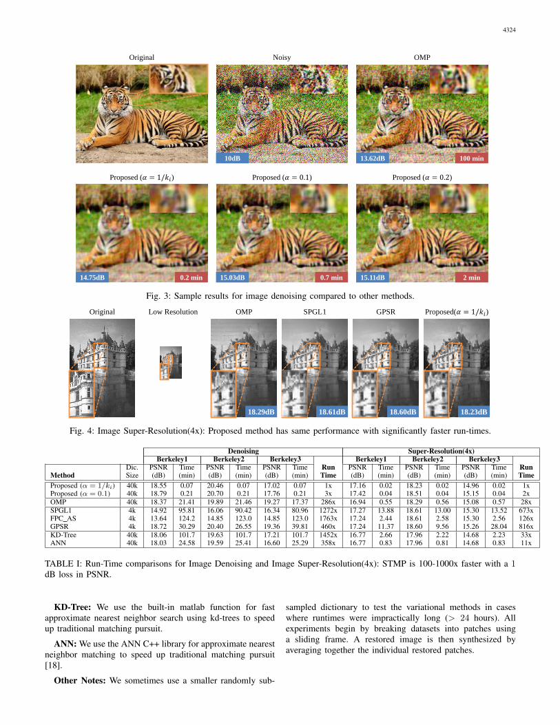
Fig. 3: Sample results for image denoising compared to other methods.

Original Low Resolution OMP SPGL 1 GPSR Proposed(𝛼 = 1/𝑘𝑖)

18.29dB 18.61dB 18.60dB 18.23dB

Fig. 4: Image Super-Resolution(4x): Proposed method has same performance with significantly faster run-times.

Denoising Super-Resolution(4x)Berkeley1 Berkeley2 Berkeley3 Berkeley1 Berkeley2 Berkeley3

Dic. PSNR Time PSNR Time PSNR Time Run PSNR Time PSNR Time PSNR Time RunMethod Size (dB) (min) (dB) (min) (dB) (min) Time (dB) (min) (dB) (min) (dB) (min) TimeProposed (α = 1/ki) 40k 18.55 0.07 20.46 0.07 17.02 0.07 1x 17.16 0.02 18.23 0.02 14.96 0.02 1xProposed (α = 0.1) 40k 18.79 0.21 20.70 0.21 17.76 0.21 3x 17.42 0.04 18.51 0.04 15.15 0.04 2xOMP 40k 18.37 21.41 19.89 21.46 19.27 17.37 286x 16.94 0.55 18.29 0.56 15.08 0.57 28xSPGL1 4k 14.92 95.81 16.06 90.42 16.34 80.96 1272x 17.27 13.88 18.61 13.00 15.30 13.52 673xFPC AS 4k 13.64 124.2 14.85 123.0 14.85 123.0 1763x 17.24 2.44 18.61 2.58 15.30 2.56 126xGPSR 4k 18.72 30.29 20.40 26.55 19.36 39.81 460x 17.24 11.37 18.60 9.56 15.26 28.04 816xKD-Tree 40k 18.06 101.7 19.63 101.7 17.21 101.7 1452x 16.77 2.66 17.96 2.22 14.68 2.23 33xANN 40k 18.03 24.58 19.59 25.41 16.60 25.29 358x 16.77 0.83 17.96 0.81 14.68 0.83 11x

TABLE I: Run-Time comparisons for Image Denoising and Image Super-Resolution(4x): STMP is 100-1000x faster with a 1dB loss in PSNR.

KD-Tree: We use the built-in matlab function for fastapproximate nearest neighbor search using kd-trees to speedup traditional matching pursuit.

ANN: We use the ANN C++ library for approximate nearestneighbor matching to speed up traditional matching pursuit[18].

Other Notes: We sometimes use a smaller randomly sub-

sampled dictionary to test the variational methods in caseswhere runtimes were impractically long (> 24 hours). Allexperiments begin by breaking datasets into patches usinga sliding frame. A restored image is then synthesized byaveraging together the individual restored patches.

4325

Original Proposed (𝛼 = 1/𝑘𝑖) Proposed (𝛼 = 0.1) Proposed (𝛼 = 0.2)

Noisy OMP SPGL1 GPSR

18.53dB 18.98dB 19.30dB

10dB 18.51dB 13.46dB 16.34dB

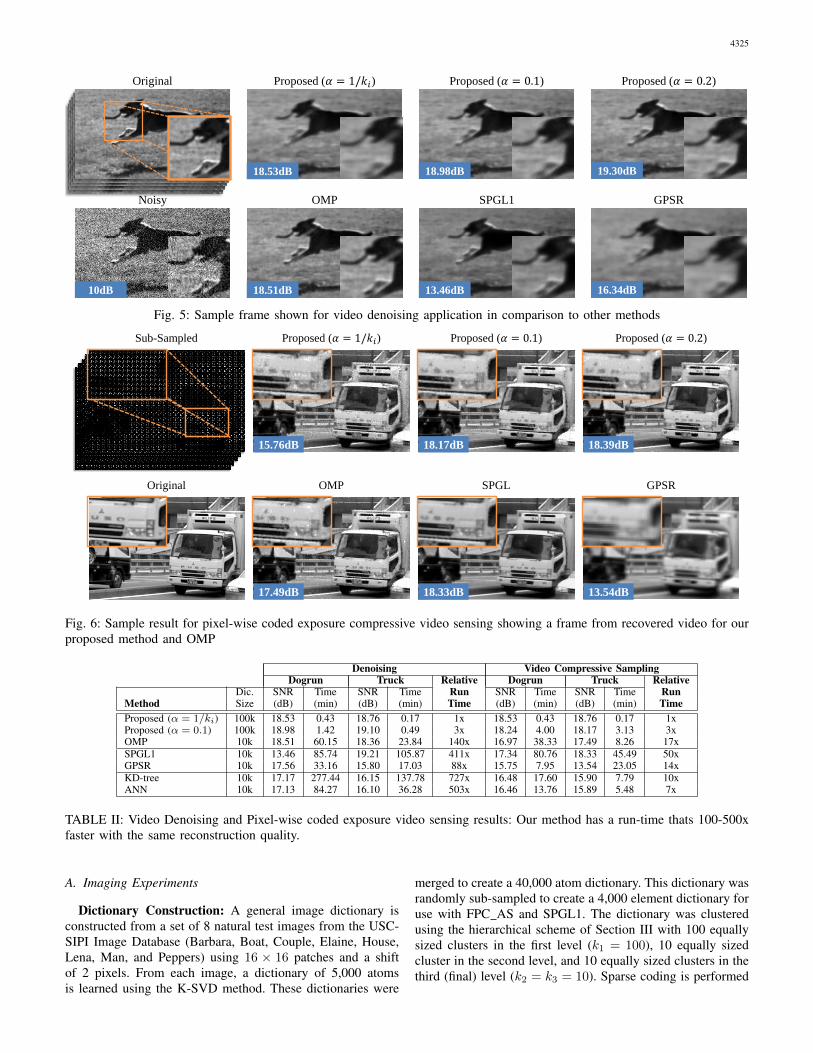
Fig. 5: Sample frame shown for video denoising application in comparison to other methods

Proposed (𝛼 = 0.1) Proposed (𝛼 = 0.2) Sub-Sampled Proposed (𝛼 = 1/𝑘𝑖)

15.76dB 18.17dB 18.39dB

SPGL GPSR OMP

17.49dB 18.33dB 13.54dB

Original

Fig. 6: Sample result for pixel-wise coded exposure compressive video sensing showing a frame from recovered video for ourproposed method and OMP

Denoising Video Compressive SamplingDogrun Truck Relative Dogrun Truck Relative

Dic. SNR Time SNR Time Run SNR Time SNR Time RunMethod Size (dB) (min) (dB) (min) Time (dB) (min) (dB) (min) TimeProposed (α = 1/ki) 100k 18.53 0.43 18.76 0.17 1x 18.53 0.43 18.76 0.17 1xProposed (α = 0.1) 100k 18.98 1.42 19.10 0.49 3x 18.24 4.00 18.17 3.13 3xOMP 10k 18.51 60.15 18.36 23.84 140x 16.97 38.33 17.49 8.26 17xSPGL1 10k 13.46 85.74 19.21 105.87 411x 17.34 80.76 18.33 45.49 50xGPSR 10k 17.56 33.16 15.80 17.03 88x 15.75 7.95 13.54 23.05 14xKD-tree 10k 17.17 277.44 16.15 137.78 727x 16.48 17.60 15.90 7.79 10xANN 10k 17.13 84.27 16.10 36.28 503x 16.46 13.76 15.89 5.48 7x

TABLE II: Video Denoising and Pixel-wise coded exposure video sensing results: Our method has a run-time thats 100-500xfaster with the same reconstruction quality.

A. Imaging Experiments

Dictionary Construction: A general image dictionary isconstructed from a set of 8 natural test images from the USC-SIPI Image Database (Barbara, Boat, Couple, Elaine, House,Lena, Man, and Peppers) using 16 × 16 patches and a shiftof 2 pixels. From each image, a dictionary of 5,000 atomsis learned using the K-SVD method. These dictionaries were

merged to create a 40,000 atom dictionary. This dictionary wasrandomly sub-sampled to create a 4,000 element dictionary foruse with FPC AS and SPGL1. The dictionary was clusteredusing the hierarchical scheme of Section III with 100 equallysized clusters in the first level (k1 = 100), 10 equally sizedcluster in the second level, and 10 equally sized clusters in thethird (final) level (k2 = k3 = 10). Sparse coding is performed

4326

using Algorithm 2.Image Denoising: Three images were selected from

the Berkeley Segmentation Dataset image numbers223061,102061, and 253027). Each image was contaminatedwith Gaussian white noise to achieve an SNR of 10dB.Greedy recovery was performed using 10 dictionary atomsper patch. Sample denoising results are shown in Figure 3.Time trial results are shown in Table I.

Image Super-resolution: This experiment enhances theresolution of an image using information from a higher reso-lution dictionary. We use three test images from the BerkeleySegmentation Database. Low resolution images are broken into4 × 4 patches. The low resolution 4 × 4 patches are mappedonto the 16× 16 dictionary patches for comparison, and thenmatched using sparse regularization algorithms 2 with sparsityK = 3. The reconstructed high-resolution patches are thenaveraged together to create a super-resolution image. Samplesuper-resolution reconstructions are shown in Figure 4. Timetrails are displayed in Table I.

B. VideoDictionary Construction: We obtained the dictionaries and

high speed videos used in [30] from the authors for thisexperiment. MP experiments were done using a dictionaryof 105 atoms, and variational experiments were done using arandomly sub-sampled dictionary of 104 atoms. Video patchesof size 7 × 7 × 9 are extracted from video frames. Thedictionary was clustered using the same parameters as theimage dictionary. Sparse coding is performed using Algorithm2 with α = 0.1.

Video Denoising: Video denoising proceeds similarly toimage denoising. The original 18 frame videos were contam-inated with Gaussian white noise to have an SNR of 10dB.Patches of size 7 × 7 × 18 were extracted from the videoto create test vectors of dimension 882. For the “dog” videopatches were generated with a shift of 1 pixel (35673 patches)while for truck a 3 pixels shift was used (14505 patches).Sparse coding and recovery was performed using 10 atomsper patch. Sample frames from denoised videos are shown inFigure 5 and runtimes are displayed in Table II.

Video Compressive Sampling: We emulate the videocompressive sampling experiments in [30]. This experimentsimulates a pixel-wise coded exposure video camera much like[30][7]. The pixel-wise coded exposure video camera operatesat 1

9 the frame-rate of the reconstructed video and thereforeresults in 1

9 samples/measurements compared to the originalvideo. For reconstruction, we closely follow the approach of[30] and reconstruct the video by using patch-wise sparsecoding using the learned dictionary. Sample frames fromreconstructed videos are shown in Figure 6 and runtimes aredisplayed in Table II.

C. Light Field AnalysisDictionary Construction: A dictionary was created for

light field patches using several sample light fields: syntheticlight fields created from the “Barbara” test image as wellas several urban scenes and light field data from the MITMedia Lab Synthetic Light Field Archive (Happy Buddha,Messerschmitt, Dice, Green Dragon, Mini Cooper, Butterfly,

Reconstru

ct

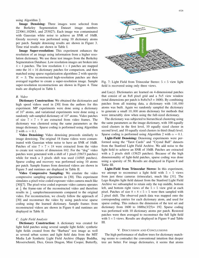
Fig. 7: Light Field from Trinocular Stereo: 5 × 5 view lightfield is recovered using only three views.

and Lucy). Dictionaries are learned on 4-dimensional patchesthat consist of an 8x8 pixel grid and a 5x5 view window(total dimensions per patch is 8x8x5x5 = 1600). By combiningpatches from all training data, a dictionary with 146, 000atoms was built. Again we randomly sampled the dictionaryto generate a small 10, 000 atom dictionary for methods thatwere intractably slow when using the full-sized dictionary.

The dictionary was subjected to hierarchical clustering usingthe same parameters as the image dictionary, with 100 equallysized clusters in the first level, 10 equally sized cluster insecond level, and 10 equally sized clusters in third (final) level.Sparse coding is performed using Algorithm 2 with α = 0.1.

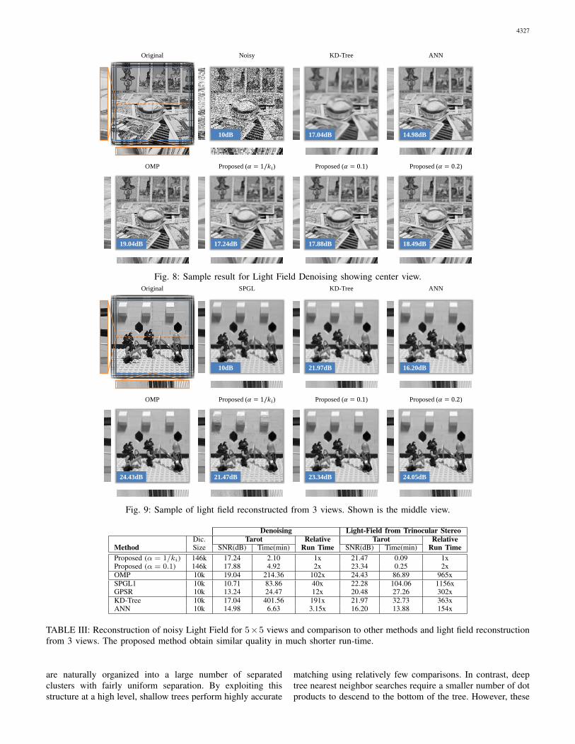
Light-Field Denoising: Denoising experiments were per-formed using the “Tarot Cards” and “Crystal Ball” datasetsfrom the Stanford Light Field Archive. We add noise to thelight field to achieve an SNR of 10dB. Patches are extractedwith a 2 pixels shift (15625 patches). Because of the highdimensionality of light-field patches, sparse coding was doneusing a sparsity of 50. Results are displayed in Figure 8 andTable III.

Light-Field from Trinocular Stereo: In this experiment,we attempt to reconstruct a light field with 5 × 5 viewsfrom just three cameras (trinocular), much like [31]. TheLego Knights light field dataset from the Stanford Light FieldArchive we subsampled to retain only the top middle, bottomleft, and bottom right views of the 5 × 5 view grid at eachpixel. Patches of size 8 × 8 × 5 × 5 were then sampled with2 pixel shift. The observed patch data was mapped onto thecorresponding entries for each dictionary atom, and used forsparse coding. This reduces the dimension of the test set anddictionary from 1600 to 1600x(3/25)= 192. Sparse codingwas performed with 10 dictionary atoms per patch. Restoredpatches were then averaged to reconstruct the full light fieldwith 5× 5 views. Results are displayed in Figure 9 and TableIII.

V. DISCUSSION AND CONCLUSIONS

The high performance of shallow trees for dictionary match-ing seems to contradict the conventional intuition that deepertree are better. For image dictionaries, it seems that atoms

4327

10dB 17.04dB 14.98dB

Original Noisy ANN KD-Tree

17.24dB 17.88dB 18.49dB

OMP Proposed (𝛼 = 1/𝑘𝑖) Proposed (𝛼 = 0.2) Proposed (𝛼 = 0.1)

19.04dB

Fig. 8: Sample result for Light Field Denoising showing center view.

10dB 21.97dB 16.20dB

Original SPGL ANN KD-Tree

21.47dB 23.34dB 24.05dB

OMP Proposed (𝛼 = 1/𝑘𝑖) Proposed (𝛼 = 0.2) Proposed (𝛼 = 0.1)

24.43dB

Fig. 9: Sample of light field reconstructed from 3 views. Shown is the middle view.

Denoising Light-Field from Trinocular StereoDic. Tarot Relative Tarot Relative

Method Size SNR(dB) Time(min) Run Time SNR(dB) Time(min) Run TimeProposed (α = 1/ki) 146k 17.24 2.10 1x 21.47 0.09 1xProposed (α = 0.1) 146k 17.88 4.92 2x 23.34 0.25 2xOMP 10k 19.04 214.36 102x 24.43 86.89 965xSPGL1 10k 10.71 83.86 40x 22.28 104.06 1156xGPSR 10k 13.24 24.47 12x 20.48 27.26 302xKD-Tree 10k 17.04 401.56 191x 21.97 32.73 363xANN 10k 14.98 6.63 3.15x 16.20 13.88 154x

TABLE III: Reconstruction of noisy Light Field for 5×5 views and comparison to other methods and light field reconstructionfrom 3 views. The proposed method obtain similar quality in much shorter run-time.

are naturally organized into a large number of separatedclusters with fairly uniform separation. By exploiting thisstructure at a high level, shallow trees perform highly accurate

matching using relatively few comparisons. In contrast, deeptree nearest neighbor searches require a smaller number of dotproducts to descend to the bottom of the tree. However, these

4328

approaches require branch-and-bound methods that backtrackup the tree and explore multiple branches in order to achievean acceptable level of accuracy. For well clustered data suchas the dictionaries considered here, the shallow tree approachachieves superior performance by avoiding the high cost ofbacktracking searches through the tree.

REFERENCES

[1] M. Elad and M. Aharon, “Image denoising via sparse and redundantrepresentations over learned dictionaries,” Image Processing, IEEETransactions on, vol. 15, no. 12, pp. 3736–3745, 2006.

[2] M. Protter and M. Elad, “Image sequence denoising via sparse andredundant representations,” Image Processing, IEEE Transactions on,vol. 18, no. 1, pp. 27–35, 2009.

[3] J. Mairal, G. Sapiro, and M. Elad, “Learning multiscale sparse represen-tations for image and video restoration,” DTIC Document, Tech. Rep.,2007.

[4] J. Yang, J. Wright, T. S. Huang, and Y. Ma, “Image super-resolution viasparse representation,” Image Processing, IEEE Transactions on, vol. 19,no. 11, pp. 2861–2873, 2010.

[5] D. Kong, M. Han, W. Xu, H. Tao, and Y. Gong, “Video super-resolutionwith scene-specific priors.” in BMVC, 2006, pp. 549–558.

[6] M. Wakin, J. Laska, M. Duarte, D. Baron, S. Sarvotham, D. Takhar,K. F. Kelly, and R. G. Baraniuk, “Compressive imaging for videorepresentation and coding,” in Picture Coding Symposium, 2006.

[7] D. Reddy, A. Veeraraghavan, and R. Chellappa, “P2c2: Programmablepixel compressive camera for high speed imaging,” in Computer Visionand Pattern Recognition (CVPR), 2011 IEEE Conference on. IEEE,2011, pp. 329–336.

[8] Y. Hitomi, J. Gu, M. Gupta, T. Mitsunaga, and S. K. Nayar, “Videofrom a single coded exposure photograph using a learned over-completedictionary,” in Computer Vision (ICCV), 2011 IEEE International Con-ference on. IEEE, 2011, pp. 287–294.

[9] K. Marwah, G. Wetzstein, Y. Bando, and R. Raskar, “Compressivelight field photography using overcomplete dictionaries and optimizedprojections,” ACM TRANSACTIONS ON GRAPHICS, vol. 32, no. 4,2013.

[10] B. Salahieh, A. Ashok, and M. Neifeld, “Compressive light field imag-ing using joint spatio-angular modulation,” in Computational OpticalSensing and Imaging. Optical Society of America, 2013.

[11] M. Li, J. Shen, and L. Jiang, “Hyperspectral remote sensing imagesclassification method based on learned dictionary,” in 2013 InternationalConference on Information Science and Computer Applications (ISCA2013). Atlantis Press, 2013.

[12] Z. Jiang, Z. Lin, and L. Davis, “Label consistent k-svd: Learning adiscriminative dictionary for recognition,” IEEE, 2013.

[13] Y. C. Pati, R. Rezaiifar, and P. Krishnaprasad, “Orthogonal matchingpursuit: Recursive function approximation with applications to waveletdecomposition,” in Signals, Systems and Computers, 1993. 1993 Con-ference Record of The Twenty-Seventh Asilomar Conference on. IEEE,1993, pp. 40–44.

[14] M. A. Figueiredo, R. D. Nowak, and S. J. Wright, “Gradient projectionfor sparse reconstruction: Application to compressed sensing and otherinverse problems,” Selected Topics in Signal Processing, IEEE Journalof, vol. 1, no. 4, pp. 586–597, 2007.

[15] E. van den Berg and M. P. Friedlander, “SPGL1: A solver for large-scalesparse reconstruction,” June 2007, http://www.cs.ubc.ca/labs/scl/spgl1.

[16] E. T. Hale, W. Yin, and Y. Zhang, “Fixed-point continuation for\ell 1-minimization: Methodology and convergence,” SIAM Journal onOptimization, vol. 19, no. 3, pp. 1107–1130, 2008.

[17] R. Gribonval, “Fast matching pursuit with a multiscale dictionary ofgaussian chirps,” Signal Processing, IEEE Transactions on, vol. 49,no. 5, pp. 994–1001, 2001.

[18] S. Arya, D. M. Mount, N. S. Netanyahu, R. Silverman, and A. Y. Wu,“An optimal algorithm for approximate nearest neighbor searching fixeddimensions,” Journal of the ACM (JACM), vol. 45, no. 6, pp. 891–923,1998.

[19] A. Andoni and P. Indyk, “Near-optimal hashing algorithms for approxi-mate nearest neighbor in high dimensions,” in Foundations of ComputerScience, 2006. FOCS’06. 47th Annual IEEE Symposium on. IEEE,2006, pp. 459–468.

[20] M. Muja and D. G. Lowe, “Fast approximate nearest neighbors withautomatic algorithm configuration.” in VISAPP (1), 2009, pp. 331–340.

[21] L. Bo, X. Ren, and D. Fox, “Hierarchical matching pursuit for imageclassification: Architecture and fast algorithms,” in Advances in NeuralInformation Processing Systems, 2011, pp. 2115–2123.

[22] L. Bo, K. Lai, X. Ren, and D. Fox, “Object recognition with hierar-chical kernel descriptors,” in Computer Vision and Pattern Recognition(CVPR), 2011 IEEE Conference on, June 2011, pp. 1729–1736.

[23] K. Yu, Y. Lin, and J. Lafferty, “Learning image representations fromthe pixel level via hierarchical sparse coding,” in Computer Vision andPattern Recognition (CVPR), 2011 IEEE Conference on, June 2011, pp.1713–1720.

[24] L. Bo, X. Ren, and D. Fox, “Multipath sparse coding using hierarchicalmatching pursuit,” in NIPS workshop on deep learning, 2012.

[25] B. Chen, G. Polatkan, G. Sapiro, D. Blei, D. Dunson, and L. Carin,“Deep learning with hierarchical convolutional factor analysis,” PatternAnalysis and Machine Intelligence, IEEE Transactions on, vol. 35, no. 8,pp. 1887–1901, Aug 2013.

[26] Z. J. Xiang, H. Xu, and P. J. Ramadge, “Learning sparse representationsof high dimensional data on large scale dictionaries,” in Advances inNeural Information Processing Systems, 2011, pp. 900–908.

[27] J.-L. Lin, W.-L. Hwang, and S.-C. Pei, “Fast matching pursuit videocoding by combining dictionary approximation and atom extraction,”Circuits and Systems for Video Technology, IEEE Transactions on,vol. 17, no. 12, pp. 1679–1689, Dec 2007.

[28] D. Needell and J. A. Tropp, “CoSaMP: Iterative signal recoveryfrom incomplete and inaccurate samples,” Applied and ComputationalHarmonic Analysis, vol. 26, no. 3, pp. 301–321, Apr. 2008. [Online].Available: http://arxiv.org/abs/0803.2392

[29] R. Rubinstein, M. Zibulevsky, and M. Elad, “Efficient implementationof the k-svd algorithm using batch orthogonal matching pursuit,” CSTechnion, 2008.

[30] D. Liu, J. Gu, Y. Hitomi, M. Gupta, T. Mitsunaga, and S. Nayar,“Efficient space-time sampling with pixel-wise coded exposure forhigh speed imaging,” Pattern Analysis and Machine Intelligence, IEEETransactions on, vol. PP, no. 99, pp. 1–1, 2013.

[31] K. Mitra and A. Veeraraghavan, “Light field denoising, light fieldsuperresolution and stereo camera based refocussing using a gmmlight field patch prior,” in Computer Vision and Pattern RecognitionWorkshops (CVPRW), 2012 IEEE Computer Society Conference on.IEEE, 2012, pp. 22–28.