5. Path-Following Algorithms - School of Mathematicsprichtar/docs/Wright-Ch5-Path-Following-Algo… · Chapter 5 Path-Following Algorithms ... (5.1d), may have multiple solutions)

Chapter 5

Path-Following Algorithms

In Chapters 1 and 2, we described the central path C, a path of points(xv , )T , s.,-) that leads to the set Sl of primal-dual solutions. Points in S2 satisfy the KKT conditions (2.4), whereas points in C are defined by conditionsthat differ from the KKT conditions only by the presence of a positive scalarparameter T > 0, namely,

A T A + s = c, (5.1a)Ax = b, (5.1b)(x, s) > 0, (5.1c)xis;, = T, i = 1, 2, ... ,n. (5.1d)

We showed in Chapter 2 that this system has a unique solution (x i , A ,-, s.,-) foreach T > 0 whenever the problem is feasible (although the KKT conditions,for which Tr = 0 in (5.1d), may have multiple solutions).

Path-following methods follow C in the direction of decreasing T to thesolution set ft They do not necessarily stay exactly on C or even particularlyclose to it. Rather, they stay within a loose but well-defined neighborhoodof C while steadily reducing the duality measure p to zero. Each searchdirection is a Newton step toward a point on C, a point for which the dualitymeasure Tr is equal to or smaller than the current duality measure Y. Thetarget value r = o u is used, where a E [0, 1] is the centering parameterintroduced in Chapter 1.

The algorithms of this chapter generate strictly feasible iterates (xk, )k sk)

that satisfy the first three KKT conditions (5.1a), (5.1b), and (5.1c). Theydeviate from the central path C only because the pairwise products xisi aregenerally not identical, so the condition (5.1d) is not satisfied exactly. This

83Dow

nloa

ded

10/0

5/15

to 1

29.2

15.1

7.18

8. R

edis

tribu

tion

subj

ect t

o SI

AM

lice

nse

or c

opyr

ight

; see

http

://w

ww

.siam

.org

/jour

nals

/ojs

a.ph

p

84 Primal-Dual Interior-Point Methods

deviation is measured by comparing the pairwise products with their averagevalue µ = x T s/n = (E xisi)/n, using, for example, a scaled norm defined by

xlsl^XSe — µe^^ = P —

(XT S e . (5.2)

IL nx^ s,^

In the literature, both the 2-norm and the 00-norm have been used in thisdefinition. For both norms, we can ensure that x and s are strictly positiveby requiring that (1/p)IIXSe — peil < 1. (If component i of x or s is zero,we have IIXSe — µe > — µl = µ.)

By using the 2-norm in (5.2) and restricting the deviation to be less thana constant 6 E [0, 1), we obtain the neighborhood N2(0) defined in (1.15):

NZ (0) = {(x, A , s) E .F° 1 (I XSe — µeí12 < Op}. (5.3)

By using the 00-norm in (5.2), we obtain the neighborhood Ná(6). We canmotivate another neighborhood A/T ('y) by noting that our chief concern isto keep the products xisi from becoming too much smaller than their averagevalue p and therefore to prevent x and s from approaching the boundary ofthe region (x, s) >_ 0 prematurely. We do not mind if some of these productsare somewhat larger than p, so the neighborhood N_ c ('y) uses a one-sidedbound on xzsi in place of the two-sided bound in (5.2), that is,

N_oo (y) _ {(x, ^, s) E ^° x2sz > yµ for all i = 1, 2, ... , n}, (5.4)

where ry E (0, 1).Path-following methods follow Framework PD of Chapter 1. They select

one of the neighborhood types .N, Nom , or N and choose the centeringparameter Q and the step length parameter a to ensure that every iterate(x k , ijk , sk ) stays within the chosen neighborhood.

Methods based on the neighborhood NZ have O(/log 1/E) complex-ity, matching the complexity estimate for the potential-reduction methodof Chapter 4 (see Corollary 4.7). We describe two such methods in thischapter: the short-step path-following algorithm (Algorithm SPF) and thepredictor-corrector algorithm (Algorithm PC). Algorithm SPF, the simplestof all interior-point methods, chooses a constant value vk - Q for the center-ing parameter and fixes the step length at Ûk - 1 for all iterations k. Thismethod was introduced by Kojima, Mizuno, and Yoshise [66] and Monteiroand Adler [94]; our analysis follows the latter paper. Algorithm PC alter-nates between two types of steps: predictor steps, which improve the valueD

ownl

oade

d 10

/05/

15 to

129

.215

.17.

188.

Red

istri

butio

n su

bjec

t to

SIA

M li

cens

e or

cop

yrig

ht; s

ee h

ttp://

ww

w.si

am.o

rg/jo

urna

ls/o

jsa.

php

Path-Following Algorithms 85

of p but which also tend to worsen the centrality measure (5.2), and cor-rector steps, which have no effect on the duality measure p but improvecentrality. Various aspects of this algorithm were foreshadowed by a num-ber of authors, including Monteiro and Adler [94] and Sonnevend, Stoer,and Zhao [122, 123], but it was first stated and analyzed in the simple formused here by Mizuno, Todd, and Ye [92]. The algorithm is sometimes called"Mizuno–Todd–Ye predictor-corrector" to distinguish it from the quite dif-ferent Mehrotra predictor-corrector algorithm of Chapter 10.

A disadvantage of the N2(0) neighborhood is its restrictive nature. Fromthe definition (5.3), we have for (x, A, s) E .N(0) that

C x2sti 1 2 02 <1-)

so that the sum of squares of all relative deviations of xisi from their averagevalue p cannot exceed 1. Even if 9 is close to its upper bound of 1, the neigh-borhood N2(0) contains only a small fraction of the points in the strictlyfeasible set .F°, so algorithms based on this neighborhood do not have muchroom in which to maneuver and the amount of progress they can achieve ateach iteration is limited. The neighborhood N(ry), on the other hand, ismuch more expansive: When ry is small, it takes up almost the entire strictlyfeasible set .F°. We discuss a long-step path-following algorithm based onthis neighborhood—Algorithm LPF—that makes more aggressive (that is,smaller) choices of centering parameter o, than does Algorithm SPF. Insteadof taking unit steps, however, Algorithm LPF performs a line search alongthe direction obtained from (1.13), choosing ak to be as large as possiblesubject to the restriction of remaining within N_ 00 (y). Algorithm LPF isclosely related to the very first polynomial primal-dual algorithm proposedby Kojima, Mizuno, and Yoshise [67]. It is more closely related to practicalalgorithms than are Algorithms SPF and PC, but its complexity bound isworse: O(n log 1 /E) vs. O(/log 1/e).

Although the kth step taken by a path-following algorithm aims for thepoint on the central path C whose duality measure is °kPk, it rarely hitsthis target. The reason is that there is a discrepancy between the nonlinearequations (5.1) and the linear approximation on which the Newton-like stepequations (1.13) are based. This discrepancy is quantified by the pairwiseproducts AxiAsz. Much of the analysis in this chapter is concerned withfinding bounds on these products and showing that the step (Oxk, OAk , A sk)

makes significant progress toward its target without actually scoring a directhit.D

ownl

oade

d 10

/05/

15 to

129

.215

.17.

188.

Red

istri

butio

n su

bjec

t to

SIA

M li

cens

e or

cop

yrig

ht; s

ee h

ttp://

ww

w.si

am.o

rg/jo

urna

ls/o

jsa.

php


In this chapter, we focus mainly on the convergence of the sequence{µk} of duality measures to zero. We close the chapter by looking at a dif-ferent, but related, issue: convergence of the primal-dual iteration sequences{(x k , A k , sk )}. We prove that the x k and sk components are bounded andthat strictly complementary solutions to (2.1), (2.2) can be recovered fromthe limit points of these sequences.

All three algorithms described in this chapter are remarkable for theirsimplicity. Despite their strong theoretical properties, they are easy to stateand to analyze, once we are past the hurdle of a few tricky technical results.They also provide the foundation for more powerful algorithms, includingalgorithms that allow infeasible starting points and rapid local convergence.Unfortunately, as we see in subsequent chapters, our claim of simple analysisdoes not necessarily hold when these capabilities are added.

The Short-Step Path-Following Algorithm

We start with the short-step path-following algorithm, Algorithm SPF.This method starts at a point (x ° , A° , s° ) E Ar2(0) and uses uniform valuesak = 1 and Uk = a, where 9 and v satisfy a certain relationship, describedbelow. All iterates (x k , A k , sk ) stay inside .N(9), and the duality measureµk converges linearly to zero at the constant rate 1 — a.

The method is defined by filling in the Framework PD from Chapter 1.We assign specific values to 0 and a, justifying them in the analysis thatfollows.

Algorithm SPFGiven 0 = 0.4, a = 1 — 0.4//, and (x ° , A ° , s°) E NZ(0);for k=0,1,2,...

set Uk = a and solve (1.13) to obtain (Oxk, AAk , A sk) ;set (xk+l, Ak +1 , (Sk+1) = (x k , Ak , sk)

1 + Qx k , AAk , ask) ;

end (for). J l l

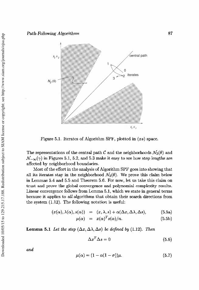
This algorithm is illustrated in Figure 5.1, which plots the first few it-erates of the algorithm projected into an unusual space. The horizontaland vertical axes represent the pairwise products x1s1 and x2s2 for thistwo-dimensional problem, so the central path is the line emanating from(0, 0) at an angle of ir/4 radians. In this (nonlinear) space, the search direc-tions transform to curves rather than straight lines. The solution is at theorigin, and the challenge facing the algorithm is to reach this point whilemaintaining the feasibility conditions Ax = b, ATA + s = c at all iterates.D

ownl

oade

d 10

/05/

15 to

129

.215

.17.

188.

Red

istri

butio

n su

bjec

t to

SIA

M li

cens

e or

cop

yrig

ht; s

ee h

ttp://

ww

w.si

am.o

rg/jo

urna

ls/o

jsa.

php


x2 5 21

N2 (e)

path

xi s '

Figure 5.1. Iterates of Algorithm SPF, plotted in (xs) space.

The representations of the central path C and the neighborhoods N2 (9) andN(ry) in Figures 5.1, 5.2, and 5.3 make it easy to see how step lengths areaffected by neighborhood boundaries.

Most of the effort in the analysis of Algorithm SPF goes into showing thatall its iterates stay in the neighborhood N2(0). We prove this claim belowin Lemmas 5.4 and 5.5 and Theorem 5.6. For now, let us take this claim ontrust and prove the global convergence and polynomial complexity results.Linear convergence follows from Lemma 5.1, which we state in general termsbecause it applies to all algorithms that obtain their search directions fromthe system (1.12). The following notation is useful:

(x(a), A(a), s(ce)) = (x, A , s) + a(Ax, AA, As), (5.5a)µ(a) = x(a)T S(a)/n. (5.5b)

Lemma 5.1 Let the step (Ax, AA, As) be defined by (1.12). Then

AxT Os = 0 (5.6)

andµ(a) = (1 — a(1 — o)». (5.7)D

ownl

oade

d 10

/05/

15 to

129

.215

.17.

188.

Red

istri

butio

n su

bjec

t to

SIA

M li

cens

e or

cop

yrig

ht; s

ee h

ttp://

ww

w.si

am.o

rg/jo

urna

ls/o

jsa.

php


Proof. The first result is left as an exercise. For the second result, weuse the third row of (1.12), namely,

SAx + X Os = — XSe + ape. (5.8)

By summing the n components of this equation, we obtain sT Ox + xT Os =—(1 — a)x T s. From this formula and (5.6), we obtain

x(o)Ts(o) = xT s + a(ST Ox + x T Os) + a2 AXT OS = xT s(1 — a(1 — a)),

giving the result. ❑For Algorithm SPF, we have by our specific choices of ak and cak that

Pk+1 = Qµk = (1 — =) µk, k = 0,1, ... , (5.9)

so global linear convergence follows. The polynomial complexity result is animmediate consequence of (5.9) and Theorem 3.2.

Theorem 5.2 Given E > 0, suppose that the starting point (x°, A ° , s° ) EA/(0.4) in Algorithm SPF has

µo < 1 /€'

for some positive constant i. Then there is an index K with K = O('log 1/c)such that

µk<6 forallk>K.

Proof. Because of (5.9), we can set 6 = 0.4 and w = 0.5 in Theorem 3.2,and the result follows immediately. ❑

In the next section, we return to the task of showing that the iterates(x k , ijk , s k ) stay inside N2(0).

Technical Results

The first result is purely technical; its proof can be found at the end ofthe chapter.

Lemma 5.3 Let u and v be any two vectors in Rn with uT v > 0. Then

IIUVeII < 2 -3/2 11u + v11 2 ,

whereU = diag(ul, u2, ... , urm,), V = diag(vl, v2,. . . , vn).D

ownl

oade

d 10

/05/

15 to

129

.215

.17.

188.

Red

istri

butio

n su

bjec

t to

SIA

M li

cens

e or

cop

yrig

ht; s

ee h

ttp://

ww

w.si

am.o

rg/jo

urna

ls/o

jsa.

php


We showed in Lemma 5.1 that the inner product Ax T As = > AxiAsiis zero, but there is no reason for the individual pairwise products to bezero. In the next result, Lemma 5.4, we find a bound on the vector of thesepairwise products.

Lemma 5.4 If (x, A, s) E N2 (0), then

AXASeII G 02+ n(1—a)2 µ23/2(1_0)

Proof. Recall the definition of the diagonal matrix D as X112S-1/2 from(1.24). If we multiply (5.8) by (XS) -1/2 , we obtain

D-1 0x + DAs = (X S) - 1 /2 (-XSe + Qµe). (5.10)

Now, apply Lemma 5.3 with u = D-1 0x and v = DAs to obtain

IIoXASeII = II (D- 'AX)(DAS)eIic 2-3/2 IID-pox + DAsII 2

= 2-3/2 11 (XS) -1/2 (—XSe+ ate) I 2n

= 2-3/2 n (— xzs + orjU)2

i=1 xisi

< 2-3/2 II XSe — aµe1I 2

mini xisi

Since (x, A , s) E M(9), we have

min xísi > (1 - B)µ.2

For a bound on the numerator in (5.11), note first that

eT (X Se - µe) = x T s - peT e = 0,

and therefore

from Lemma 5.3from (5.10)

(5.11)

(5.12)

IIXSe — aµeII 2

= II(XSe—µe)+( 1 —a)µell 2

= IIXSe-µe11 2 +2(1 -a)peT (XSe-µe)+(1 -a) 2 92 eT e< 02ti2 + (1 - o) 2µ2n. (5.13)D

ownl

oade

d 10

/05/

15 to

129

.215

.17.

188.

Red

istri

butio

n su

bjec

t to

SIA

M li

cens

e or

cop

yrig

ht; s

ee h

ttp://

ww

w.si

am.o

rg/jo

urna

ls/o

jsa.

php


We obtain the result by substituting (5.12) and (5.13) into (5.11). ❑Lemma 5.10 is a result similar to Lemma 5.4 that is proven during our

analysis of Algorithm LPF. Lemma 5.4 gives a tighter bound, however, be-cause the current point (x, A, s) lies in the more restrictive neighborhoodN2(9). The difference in the bounds obtained in Lemmas 5.4 and 5.10 ac-counts for the difference in polynomial complexity estimate for AlgorithmsSPF and LPF.

We know from Lemma 5.1 that p decreases linearly as we move alongthe direction (Ax, AA, As). But how far does the point (x(a), A(a), s(a))stray from the central path in the 2-norm measure? The answer is providedby the following result, which is a simple consequence of Lemma 5.4.

Lemma 5.5 If (x, A , s) E N2(0), we have

IIX(a)S(a)e — p(a)eII< 11— aI IIXSe — ,ell + a2 II 1XASeII (5.14a)

< Il— albµ+a2 02 +n(1 —Q)2j ii . (5.14b)

23/2 (1 — 0)

Proof. We use the third row of (1.12) to resolve the components ofX(a)S(a)e — p(a)e. From this equation and Lemma 5.1, we have

x(a)s(a) — µ(a)= xisi + a(si0xi + xizsi) + a2 0xi0si — (1 — a(1 — Q))µ= x-s(1 — a) + amµ + a2 0xi0si — (1 — a + av»C= xisi(1 — a) + JAX,Asi — (1 — a)µ.

Reassembling these components into a vector, we obtain

IIX(a)S(a)e — µ(a)eII

II Lxisi(1 — a) — (1 — a)µ + a20xZOsi I i l

< I1— al II XSe — µell + a2 IIzXASell

I1 — al 0p + a2 02 -1- n(1 — v)2

µ. ❑23/2(1_0)

Theorem 5.6 defines a relationship between 0 and a and shows that evena full step (a = 1) along the search direction will not take the new iterateoutside the neighborhood N2(0).D

ownl

oade

d 10

/05/

15 to

129

.215

.17.

188.

Red

istri

butio

n su

bjec

t to

SIA

M li

cens

e or

cop

yrig

ht; s

ee h

ttp://

ww

w.si

am.o

rg/jo

urna

ls/o

jsa.

php


Theorem 5.6 Let the parameters 0 E (0, 1) and a E (0, 1) be chosen tosatisfy

02+n(1 —a)2 o'0. (5.15)23/2 (1 — 0)

Then if (x, A , s) E N2 (9), we have

(x(a), A(a), s(a)) E N2(0)

for all a E [0,1].

Proof. Substituting (5.15) into (5.14b), we have for a E [0, 1] that

IIX(a)S(a)e — p(a)eJJ < (1 — a)Bµ + a2Q0µ< (1 — a + aa)0µ since a E [0,1]

= 0µ(a) from (5.7). (5.16)

Hence the point (x(a), )(a), s(a)) satisfies the proximity condition for f2(0).We still have to check that (x(a), )t(a), s(a)) E .F°. It is easy to verify

that Ax(a) = b, AT A(a) + s(a) = c.

To check the positivity condition (x(a), s(a)) > 0, note first that (x, s) _(x(0), s(0)) > 0. It follows from (5.16) that

xi(a)s2(a) > (1 — 0)u(a) = (1 — 0)(1 — a(1 — v))µ > 0, (5.17)

where the strict inequality is a consequence of 0 E (0, 1), a E (0, 1], andor E (0, 1). Hence, we cannot have xi(a) = 0 or s(a) = 0 for any indexi when a E [0, 1]. Therefore (x(a), s(a)) > 0 for all a E [0, 1], and so(x(a), A(a), s(a)) E F°, as claimed. ❑

At this point, the proof of validity of Algorithm SPF is nearly complete.It remains only to check that our specific choice of parameters 0 and a,namely,

9 = 0.4, a= 1-0.4/ / ,

satisfies the condition (5.15) for all n > 1. We leave this as an exercise.

The Predictor-Corrector Method

In Algorithm SPF, we chose aj - o to lie strictly between 0 and 1.This choice achieves the twin goals of improving centrality and reducingthe duality measure µ into a single step. The predictor-corrector method,D

ownl

oade

d 10

/05/

15 to

129

.215

.17.

188.

Red

istri

butio

n su

bjec

t to

SIA

M li

cens

e or

cop

yrig

ht; s

ee h

ttp://

ww

w.si

am.o

rg/jo

urna

ls/o

jsa.

php


Algorithm PC, takes two different kinds of steps to achieve each of thesetwo goals. Successive iterations of Algorithm PC alternate between the twotypes of steps, which are

• predictor steps (Uk = 0) to reduce p,

• corrector steps (Qk = 1) to improve centrality.

The other important ingredient in Algorithm PC is a pair of N2 neighbor-hoods, nested one inside the other. Even-index iterates ((x k , A k , s k ), withk even) are confined to the inner neighborhood, whereas odd-index iteratesare allowed to stray into the outer neighborhood, but not beyond.

The term predictor-corrector arose because of the analogy with predictor-corrector algorithms in ordinary differential equations (ODEs). These algo-rithms follow the solution trajectory of an initial-value ODE problem byalternating between predictor steps (which move along a tangent to the tra-jectory) and corrector steps (which move back toward the trajectory fromthe predicted point).

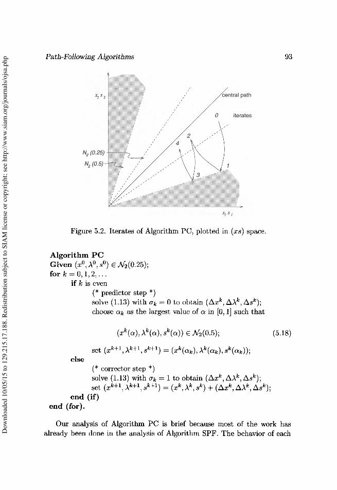
We examine the first two iterations of Algorithm PC, which suffice toillustrate the whole algorithm. Starting from a point (x ° , A° , s° ) in the innerneighborhood, we calculate a predictor step by setting oo = 0. We movealong this direction until we reach the boundary of the outer neighborhood.We stop at this point and define the new iterate (x', A, s'). A corrector stepis now calculated by setting al = 1. A unit step along this direction (a = 1)leads to a new iterate (x 2 , A 2 , s2 ) that is back inside the inner neighborhood.The two-step cycle then repeats, generating a sequence of iterates with theeven-index iterates inside the inner neighborhood and the odd-index iterateson the boundary of the outer region. See Figure 5.2 for a depiction of thisprocess.

Predictor steps reduce the value of p by a factor of (1 — a), where a isthe step length. Corrector steps leave p unchanged, but by moving back intothe inner neighborhood, they give the algorithm more room to maneuver onthe next (predictor) iteration.

We obtain a formal specification of Algorithm PC by again filling inFramework PD of Chapter 1. For simplicity, we define the inner neigh-borhood to be M(0.25) and the outer neighborhood to be J(0.5). Otherchoices are possible, provided that the two neighborhoods are related to eachother in a way that we define below.

Dow

nloa

ded

10/0

5/15

to 1

29.2

15.1

7.18

8. R

edis

tribu

tion

subj

ect t

o SI

AM

lice

nse

or c

opyr

ight

; see

http

://w

ww

.siam

.org

/jour

nals

/ojs

a.ph

p


4

xZ s 2 central path

0 iterates

24

N2 (0.25)

2(0.5)

x^s I

Figure 5.2. Iterates of Algorithm PC, plotted in (xs) space.

Algorithm PCGiven (x° , )°, s°) E 2(0.25);for k=0,1,2,...

if k is even(* predictor step *)solve (1.13) with vk = 0 to obtain (Axk, OAk , Ask) ;

choose ak as the largest value of a in [0, 1] such that

(x k (a), A k (a), sk (a)) E A/(0.5); (5.18)

set (x'', A' 4 , sk+1 ) = (x k (ak), A k (ak), sk (ak)) ;else

(* corrector step *)solve (1.13) with Qk = 1 to obtain (Oxk, AAk , A sk) ;set (xk+l , Ak+1 , 8k+1) = (xk , Ak , sk ) + (Oxk , A á k , Ask );

end (if)end (for).

Our analysis of Algorithm PC is brief because most of the work hasalready been done in the analysis of Algorithm SPF. The behavior of eachD

ownl

oade

d 10

/05/

15 to

129

.215

.17.

188.

Red

istri

butio

n su

bjec

t to

SIA

M li

cens

e or

cop

yrig

ht; s

ee h

ttp://

ww

w.si

am.o

rg/jo

urna

ls/o

jsa.

php


predictor step is described by the following lemma, which finds a lower boundon its step length and therefore an estimate of the reduction in µ.

Lemma 5.7 Suppose that (x, A, s) E.2(0.25), and let (Ox, AA, Os) be cal-culated from (1.12) with a = 0. Then (x(a), A(a), s(a)) E N2(0.5) for alla E [0, á], where

1/2Ee = min l (5.19)

2 ' 8^JAXOSeIIl

Hence, the predictor step has length at least d, and the new value of p is atmost (1 — á)µ.

Proof. Fiom (5.14a), we have

IX(a)S(a)e — µ(a)eII< (1 — a)IIXSe — peil + a2 IIAXOSell< (1 — a)IIXSe — peil + 8llOXOSeII ll LX /Sell from (5.19),

8(1< 4 (1 — a)µ + 1 (1 — a)µ since (x, A , s) E N2(0.25),— — a)

< 4 (1 — a)µ + 4 (1 — a)µ since a < 2,< 2µ(a) by (5.7), with a = 0.

Hence, the point (x(a), A(a), s(a)) satisfies the proximity condition for A/(0.5).The remaining strict feasibility conditions can be verified as in the proof ofTheorem 5.6. ❑

Lemma 5.4 can be used to find a lower bound on a. Setting 0 = 0.25and a = 0 in this result, we obtain

µ > 2"(1-0.25) — 3^ > 0.168II/XOSell — 8((0.25) 2 + n) 1 + 16n — n

since n > 1. Hence, from (5.19) we have

2, ( 0.16 1 1/2 0.4a > min l =

n ;7•

Since predictor steps are taken at even-index iterates, this bound impliesthat

< 0.4 1 / 2k+1_ (1_/2k, k=0,2,4 .... (5.20)D

ownl

oade

d 10

/05/

15 to

129

.215

.17.

188.

Red

istri

butio

n su

bjec

t to

SIA

M li

cens

e or

cop

yrig

ht; s

ee h

ttp://

ww

w.si

am.o

rg/jo

urna

ls/o

jsa.

php


Corrector steps are described by the following lemma, which shows thatthey return any point in .N(0.5) to the inner neighborhood M(0.25) withoutchanging the value of p.

Lemma 5.8 Suppose that (x, A , s) E .2(0.5), and let (Ox, AA, Os) be cal-culated from (1.12) with a = 1. Then we have

(x(1), X(1), s(1)) E A/(0.25), µ(1) = p.

Proof. By substituting v = 1 into (5.7), we have immediately that a(1) _p. (In fact, µ(a) = µ for all a E [0,1].)

By substituting 0 = 0.5, a = 1, and a = 1 into (5.14b), we find that

IIX(1)S(1)e — µ(1)eJI <t/4 = µ(1)/4.

Hence, (x(1), A(1), s(1)) satisfies the proximity conditions for .2(0.25). Theproof is completed by verifying that (x(1), A(1), s(1)) is also strictly feasible,which follows as in Theorem 5.6. 0

As we see from this lemma, corrector iterations leave the value of theduality measure µ unchanged. However, because the predictor iterationsachieve a substantial reduction in p (5.20), we can prove the same kind ofpolynomial complexity result as for the short-step algorithm.

Theorem 5.9 Given e > 0, suppose that the starting point (x°, A°, sc) E.2(0.25) in Algorithm PC has

µo < 1 /E'`

for some positive constant ic. Then there is an index K with K = O(,/ log 1/c)such that

Ilk<E forallk>K.

Proof. Combining (5.20) with Lemma 5.8, we have

( 0.4\11k+2 = µk+1 (1— J µk , k = 0, 2, 4, ... .

Hence, the reduction requirement (3.10) of Theorem 3.2 is almost satisfiedwhen we set 6 = 0.4 and w = 0.5, except that the reduction in p occursover a span of two iterations instead of just one. The proof of Theorem 3.2can be modified easily to handle this slightly different condition (as weD

ownl

oade

d 10

/05/

15 to

129

.215

.17.

188.

Red

istri

butio

n su

bjec

t to

SIA

M li

cens

e or

cop

yrig

ht; s

ee h

ttp://

ww

w.si

am.o

rg/jo

urna

ls/o

jsa.

php


showed in the exercises for Chapter 3) without affecting the conclusion ofthe theorem. ❑

The predictor-corrector algorithm is a definite improvement over theshort-step algorithm because of the adaptivity that is built into the choice ofpredictor step length. In Algorithm SPF, the values of v and a are fixed atconservative values so that they confine the iterates (x k , Ak , sk ) to the neigh-borhood A/(û) under all circumstances. By contrast, the predictor steplengths of Algorithm PC are longer when the predictor direction is a goodsearch direction, that is, when it produces a large reduction in p withoutmoving away from the central path too rapidly. During the final stages of thealgorithm, the predictor directions become better and better, and AlgorithmPC is eventually able to use step lengths close to 1. In fact, convergence ofthe duality measures µk to zero is superlinear, as we see in Chapter 7.

Despite its adaptivity, Algorithm PC is still restricted by the crampednature of the N2 neighborhoods, particularly during early iterations whenfar from the solution. We now describe a long-step path-following algorithmthat combines flexibility in the choice of step length with the use of a moreliberal neighborhood N_,,(y).

A Long-Step Path-Following Algorithm

Algorithm LPF generates a sequence of iterates in the neighborhoodN— m (ry), which, for small values of y (say, y = 10-3 ), occupies most ofthe set .F° of strictly feasible points. At each iterate of Algorithm LPF, wechoose the centering parameter Uk to lie between the two fixed limits Aminand Um , where 0 < Umin < amax < 1. The search direction is, as usual,obtained by solving (1.13), and we choose the step length ak to be as largeas possible, subject to staying inside (y).

A formal statement of the algorithm follows.

Algorithm LPFGiven y, Umin, Umax with 'y E (0, 1), 0 < Umin < Umax < 1,

and (x°, A ° , s° ) E N m ('y);for k=0,1,2,...

choose ak E [amin, umax];solve (1.13) to obtain (Ox', AA k , Ask );choose ak as the largest value of a in [0, 1] such that

(x k (a), A c (a), sk (a)) E Ar

o('Y); (5.21)Dow

nloa

ded

10/0

5/15

to 1

29.2

15.1

7.18

8. R

edis

tribu

tion

subj

ect t

o SI

AM

lice

nse

or c

opyr

ight

; see

http

://w

ww

.siam

.org

/jour

nals

/ojs

a.ph

p


X2 S 2 path

XIS'

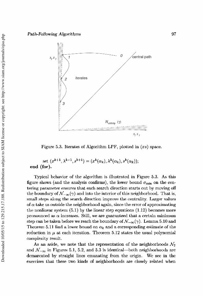
Figure 5.3. Iterates of Algorithm LPF, plotted in (xs) space.

set (x' +i ),k+1, sk+l ) = (x k (ak), A k (ak), sk (ak));end (for).

Typical behavior of the algorithm is illustrated in Figure 5.3. As thisfigure shows (and the analysis confirms), the lower bound m;fl on the cen-tering parameter ensures that each search direction starts out by moving offthe boundary of N_^ (y) and into the interior of this neighborhood. That is,small steps along the search direction improve the centrality. Larger valuesof a take us outside the neighborhood again, since the error of approximatingthe nonlinear system (5.1) by the linear step equations (1.12) becomes morepronounced as a increases. Still, we are guaranteed that a certain minimumstep can be taken before we reach the boundary of N_^ (ry). Lemma 5.10 andTheorem 5.11 find a lower bound on aj and a corresponding estimate of thereduction in p at each iteration. Theorem 5.12 states the usual polynomialcomplexity result.

As an aside, we note that the representation of the neighborhoods .NZand .N_,, in Figures 5.1, 5.2, and 5.3 is identical—both neighborhoods aredemarcated by straight lines emanating from the origin. We see in theexercises that these two kinds of neighborhoods are closely related whenD

ownl

oade

d 10

/05/

15 to

129

.215

.17.

188.

Red

istri

butio

n su

bjec

t to

SIA

M li

cens

e or

cop

yrig

ht; s

ee h

ttp://

ww

w.si

am.o

rg/jo

urna

ls/o

jsa.

php

98

Primal-Dual Interior-Point Methods

n = 2 but that this relationship breaks down for larger values of n. Thetwo neighborhoods NZ and would have different shapes if we extendedFigures 5.1, 5.2, or 5.3 into a third dimension.

Lemma 5.10 If (x, A , s) E then

IDXASelI <23/2(1 + 1 /y)nµ.

Proof. As in the proof of Lemma 5.4, we have

JAXASelI < 2-312 11(XS) -12 (—XSe + ape)11 2 .

Expanding the squared Euclidean norm and using such relationships asxT s = np and eT e = n, we obtain

OXOSe 2-3^ — X S 1/2e + Q X S 1 ^2 2II II < 2— O ( ) µ( ) e^^n

< 2-3/2 XT s - 2QµeT e +Q2µ2 ^z= 1 xisi

<_ 2-3 '2 xT s - 2QµeT e + Q2 µ2 n 1I since xis2 > yµ

yµ2

< 2-3^2 1 - 2cr + np,y ]

< 2-3/2 (1 + 1/y)np,

as claimed. ❑

Theorem 5.11 Given the parameters y, amin , and am in Algorithm LPF,there is a constant S independent of n such that

µk+l: (1- n)µk

for all k > 0.

Proof. We start by proving that

(xk (a), Ak (a), sk (a)) E (y) for all a E [0, 23/2y 1 + y n ] , (5.22)

from which we deduce that ak is bounded below as follows:

> 23/2 0k 1Y (5.23)Dow

nloa

ded

10/0

5/15

to 1

29.2

15.1

7.18

8. R

edis

tribu

tion

subj

ect t

o SI

AM

lice

nse

or c

opyr

ight

; see

http

://w

ww

.siam

.org

/jour

nals

/ojs

a.ph

p


For any i = 1, 2, .. . , n, we have from Lemma 5.10 that

AxkLsZ I < IIAXkASke II2 <23'2(1 + 1/ry)nµk. (5.24)

Using (5.8), we have from xksk > -yµ, and (5.24) that

x(a)s(a) = (xi + aAxk)(sk + a. s)= xks + a(x^Ask + skAxk) + a2 0xkOsk>_ xks,(1 — a) + aak/Lk — a2 I x%Osk)> 'y(1 — a)µk + aak/lk — a2 2 -3/2 (1 + 1/-y)nµk•

Meanwhile, we have from (5.7) that

µk(a) = (1 - a(1 - ak))µk•

From these last two formulas, we can see that the proximity condition

xk(a)s (a) ^ Wtk(a)

is satisfied, provided that

'y(1 - a)µ + aaik - a22-3/2 (1 + 1 /7)npk ? 7( 1 - a + acrk)µk•

Rearranging this expression, we obtain

aakµk( 1 - 'Y) ? a22-3/2nµk( 1 + 1/'Y),

which is true if23/2 1-7

a< n Qky l+ry

We have proved that (x k (a), A k (a), sk(a)) satisfies the proximity conditionfor T(y) when a lies in the range stated in (5.22). We can also show, asin the proof of Theorem 5.6, that (xk (a), A k (a), sk (a)) E .F° for all a in thegiven range. Hence, we have proved (5.22) and therefore (5.23).

We complete the proof of the theorem by estimating the reduction in µon the kth step. From (5.7) and (5.23), we have

/Lk+1 = (1 — ak(1 — Qk))Nlk3/2

< 1 - 2 7 1-7ak(1-Qk) µk. (5.25)n 1+ryD

ownl

oade

d 10

/05/

15 to

129

.215

.17.

188.

Red

istri

butio

n su

bjec

t to

SIA

M li

cens

e or

cop

yrig

ht; s

ee h

ttp://

ww

w.si

am.o

rg/jo

urna

ls/o

jsa.

php


Now, the function a(1 — v) is a concave quadratic function of v, so on anygiven interval it attains its minimum value at one of the endpoints. Hence,we have

ak(1—ak) > min {amin( 1 — amin), amax( 1 — Umax)} for all ak E [amin, amax]•

The proof is completed by substituting this estimate into (5.25) and setting

S = 23/2 ry 1 — 2 min {amin( 1 — amin), amax( 1 — am )}. ❑7

The complexity result is an immediate consequence of Theorems 5.11and 3.2.

Theorem 5.12 Given E > 0 and -y E (0, 1), suppose that the starting point(x ° , A ° , s° ) E N(ry) in Algorithm LPF has

Ito < 1 /E'

for some positive constant ic. Then there is an index K with K = O(n log 1/e)such that

µk<E forallk>K.

Limit Points of the Iteration Sequence

The convergence results of this chapter have focused thus far on con-vergence of the sequence {µk} to zero, without saying anything about thesequence of iterates { (x k , ) k , sk ) } . The behavior of the iterate sequence is alittle more complicated than one might expect. The main issue is to showthat the sequence {(x k , sk )} has a limit point, because we can construct aprimal-dual solution from any such limit point by the following argument:If K is the subsequence for which limk EK(x k , sk ) = (x*, s*), we have for allkEKthat

Ax k = b, c — sk E Range(AT ), (xk, sk) > 0.

Taking limits and using the facts that Range(AT ) is closed and Ak j 0, wefind that (x*, s*) satisfies

Ax* = b, c — s* E Range(AT ), (x*, s*) > 0, (x *)T s* = 0.Dow

nloa

ded

10/0

5/15

to 1

29.2

15.1

7.18

8. R

edis

tribu

tion

subj

ect t

o SI

AM

lice

nse

or c

opyr

ight

; see

http

://w

ww

.siam

.org

/jour

nals

/ojs

a.ph

p


Hence, c — s* = AA* for some A'. Comparing these conditions with the KKTconditions (1.4), we conclude that (x*, A*, s*) E S2 as claimed.

In this section, we look at the limiting behavior of the sequence {(x c , sic)}generated by each algorithm in this chapter. We show that the sequence isbounded and therefore has at least one limit point. Further, all limit pointscorrespond to strictly complementary solutions, that is, solutions (x*, A*, s*)for which

xi > 0 (i E B), si > 0 (i E N), (5.26)

where B U N is the partition of {1, 2, ... , n} defined in (2.11).

Lemma 5.13 Let po > 0 and ry E (0, 1). Then for all points (x, A , s) with

(x, A, s) E N ^('Y) C F' µ < µo (5.27)

(where p = x T s/n), there are constants Co and C3 such that

II (x, s) II <_ Co, (5.28) 0 < xi < p/C3 (i E N), 0 < si < p/C3 (i E B), (5.29) Si > C3'y (i E N), xi > C3ry (i E B). (5.30)

Proof. The first result (5.28) follows immediately from Lemma 2.5 if weset K = npo.

For (5.29) and (5.30), let (x*, A*, s*) be any primal-dual solution. Sincethis solution and the point (x, A, s) are both feasible, we have

Ax = Ax* = b, ATA +s= ATA* +s* =

therefore

(x — x* ) T (s — s * ) = —(x — x* ) T AT (íA — A* ) = 0.

Since (2.11) implies that xi = 0 for i E N and si = 0 for i E B, we canrearrange this expression to obtain

np = x T s* + sT x * = E xisi + i: six'. iEJ%/ iE13

Since each term in the summations is nonnegative, each term is bounded bynp. Hence, for any i E N with si > 0, we have

0<xis2 <np = 0<xi< np. (5.31)siD

ownl

oade

d 10

/05/

15 to

129

.215

.17.

188.

Red

istri

butio

n su

bjec

t to

SIA

M li

cens

e or

cop

yrig

ht; s

ee h

ttp://

ww

w.si

am.o

rg/jo

urna

ls/o

jsa.

php


Since the expression (5.31) holds for any solution (x*, )*, s*) with si > 0,we choose the one that yields the tightest bound on xi, that is,

n0<xi< *µ.

sup(A* y *) EcD si

Taking the maximum of this bound over the indices i E N, we obtain

nmax xi < µ.iEiv miniENsuP(A*,s*)ES2p sZ

Similarly,0<maxsi< n µ

iE6 miniEB SUPX*ES2p xiCombining the two estimates, we obtain

max max xi, max si < n min min sup x, min sup si µiEJV ic-B ) iEB x*Elp iE. (A* s* ) ES D_ n

E(A, b, c) µ'

where e(A, b, c) was defined in (3.5). The result (5.29) follows immediatelywhen we set

e(A b c)C3 = (5.32)

n

Existence of a strictly complementary solution (Theorem 2.4) guaranteesthat e(A, b, c) > 0, so C3 is positive.

Finally, since (x, A , s) E N_oo(y), we have xisi >_ ryµ for all i = 1, 2, ... , n.Hence, we have from (5.29) that

Si? yµ _> rye` = C3y for all i E N.xi µ/C3

In the same way, we can show that xi > C3ry for i E B, proving (5.30). 0

Theorem 5.14 Let {(x k , .fik , sk )} be a sequence of iterates generated by Algorithm SPF, PC, or LPF, and suppose that Pk J, 0 as k —+ oo. Then thesequence {(xk , sk )} is bounded and therefore has at least one limit point.Each limit point corresponds to a strictly complementary primal-dual solu-tion.D

ownl

oade

d 10

/05/

15 to

129

.215

.17.

188.

Red

istri

butio

n su

bjec

t to

SIA

M li

cens

e or

cop

yrig

ht; s

ee h

ttp://

ww

w.si

am.o

rg/jo

urna

ls/o

jsa.

php


Proof. All three algorithms confine their iteration sequences to a neigh-borhood N-oo (y) for some ry > 0. In Algorithm SPF, we have

(x k , A k , sk ) E.M2(0.4) C N_oo (0.4).

In Algorithm PC, all iterates belong to N2(0.5), which is a subset of N_á (0.5),whereas in Algorithm LPF, the value of ry is chosen explicitly. Also, the se-quences {µk} are nonincreasing for each method; in particular, µk <_ µofor all k > 0. Hence each iterate (x k , A k , sk ) satisfies the assumptions ofLemma 5.13.

Boundedness of {(x k , sk )} follows from (5.28). If (x*, s*) is a limit point,we can find A* such that (x*, A*, s*) E 11 (see the discussion above).Because of (5.30), we must have

s, >C3y>0 (iEN), x%>C3y>0 (i13),

so the solution is strictly complementary. ❑When the problem has a unique primal-dual solution (x*, A*, s*), it fol-

lows immediately from Theorem 5.14 that the iteration sequences for allthree algorithms converge to this point.

Proof of Lemma 5.3

We return to the technical lemma stated earlier in the chapter, whichclaimed that for any vector pair u, v with uT v > 0, we have

IIUVeII <_ 2-3/2 11u + v11 2

First, note that for any two scalars a and 3 with a,3 > 0, we have from thealgebraic-geometric mean inequality that

1 2Ia + /3I. (5.33)

Since uT v > 0, we have

0 < uT V = uivi + E uivi = l uivi l - juivi I , (5.34)uiv;>O uivz<0 iEP iEM

where we partitioned the index set {1, 2, ... , n} as

P={i1uivi>0}, M ={ iI uivi <0}.Dow

nloa

ded

10/0

5/15

to 1

29.2

15.1

7.18

8. R

edis

tribu

tion

subj

ect t

o SI

AM

lice

nse

or c

opyr

ight

; see

http

://w

ww

.siam

.org

/jour

nals

/ojs

a.ph

p

104

Primal-Dual Interior-Point Methods

Now,

IIUVeII = (II [ujvi]iEPII 2 + II[uivi]iEMII 2) 1/2

2<_ (II [uivi]iEP II1 + II [uivi]iEM Ii l) 1/2 since 11 • 11 2 < 11 • Iii

<_ (2 II[uivi]iEP112)1/2 from (5.34)

< V I (u2 -f- vi) 2J ( from (5.33)sEP 1

= 2-3/2 >(u + vi) 2iEPn

< 2-3/2 ^(ui + vi) 2i=1

= 2-3/2 11u + v11 2 ,completing the proof.

Notes and References

Xu [152] has described a way to avoid the tight confines of the neigh-borhood N2(0), 0 < 1 without sacrificing O(-/hL) complexity. He uses theneighborhood N2(0) n N-.('y), where -y > 0 is small but 0 may be muchlarger than 1. Steps in this neighborhood can be almost as long as in theneighborhood alone, and the strategy has been successfully imple-mented by Xu, Hung, and Ye [153].

Lemma 5.13 and Theorem 5.14 are due to Guler and Ye [50]. The setof limit points of {(x", s k )} actually forms a continuum (see Tapia, Zhang,and Ye [126, Theorem 4.1]). Convergence of {(x k , sk )} is discussed furtherin Chapters 6 and 7.

Exercises

1. Check that the choices of 0 and o used in Algorithm SPF satisfy therelationship (5.15).

2. Prove (5.6). Does this result still hold for the infeasible step (1.20)?

3. For a given 0 E (0, 1), the problem of finding a value of a that satis-fies (5.15) while maximizing the decrease in µ for a unit step can beposed as a simple constrained optimization problem. Write down thisproblem. Does this problem have a solution for all 0 E (0, 1)? Explain.

Dow

nloa

ded

10/0

5/15

to 1

29.2

15.1

7.18

8. R

edis

tribu

tion

subj

ect t

o SI

AM

lice

nse

or c

opyr

ight

; see

http

://w

ww

.siam

.org

/jour

nals

/ojs

a.ph

p


4. Theorem 5.6 shows that the unit step for Algorithm SPF keeps thenew iterate inside the neighborhood N2(0). Express the problem offinding the maximal a such that IIX(a)S(a)e — µ(a)eI^2 G_ 0µ(a) as aquartic polynomial in a.

5. In Algorithms SPF and LPF, is there any benefit to taking a stepof length longer than 1, if such a step remains inside the requiredneighborhood?

6. In Algorithm PC, we chose the inner and outer neighborhoods to be.2(0.25) and .2(0.5), respectively. In this exercise, you are asked toconsider more general neighborhoods N2(0in) and J'12(eout) and lookfor conditions on the scalars Bi„ and °out for which the analysis of thealgorithm continues to hold.

(i) Redefine the lower bound á on the predictor step length obtainedin Lemma 5.7 for arbitrary values of Bin and Bout . That is, find avalue rl such that

( i/z=min 2' ( IIAXASe^^ )

(ii) Modify the analysis of Lemma 5.8 to find the relationship betweenBin and 0o„t that guarantees that the corrector step returns to theinner neighborhood.

(iii) What is the largest value of fl out for which the gin of part (ii)satisfies Bi„ E (0, 0o„t )?

7. Prove that when n = 2, the neighborhoods N2(0) and N_á(1— 0/^)are identical. Does a similar relationship hold when n = 3?

Dow

nloa

ded

10/0

5/15

to 1

29.2

15.1

7.18

8. R

edis

tribu

tion

subj

ect t

o SI

AM

lice

nse

or c

opyr

ight

; see

http

://w

ww

.siam

.org

/jour

nals

/ojs

a.ph

p

Documents

5. Path-Following Algorithms - School of Mathematicsprichtar/docs/Wright-Ch5-Path-Following-Algo… · Chapter 5 Path-Following Algorithms ... (5.1d), may have multiple solutions)