Embed Size (px)
Citation preview
Stanford Rock Physics Laboratory - Gary Mavko
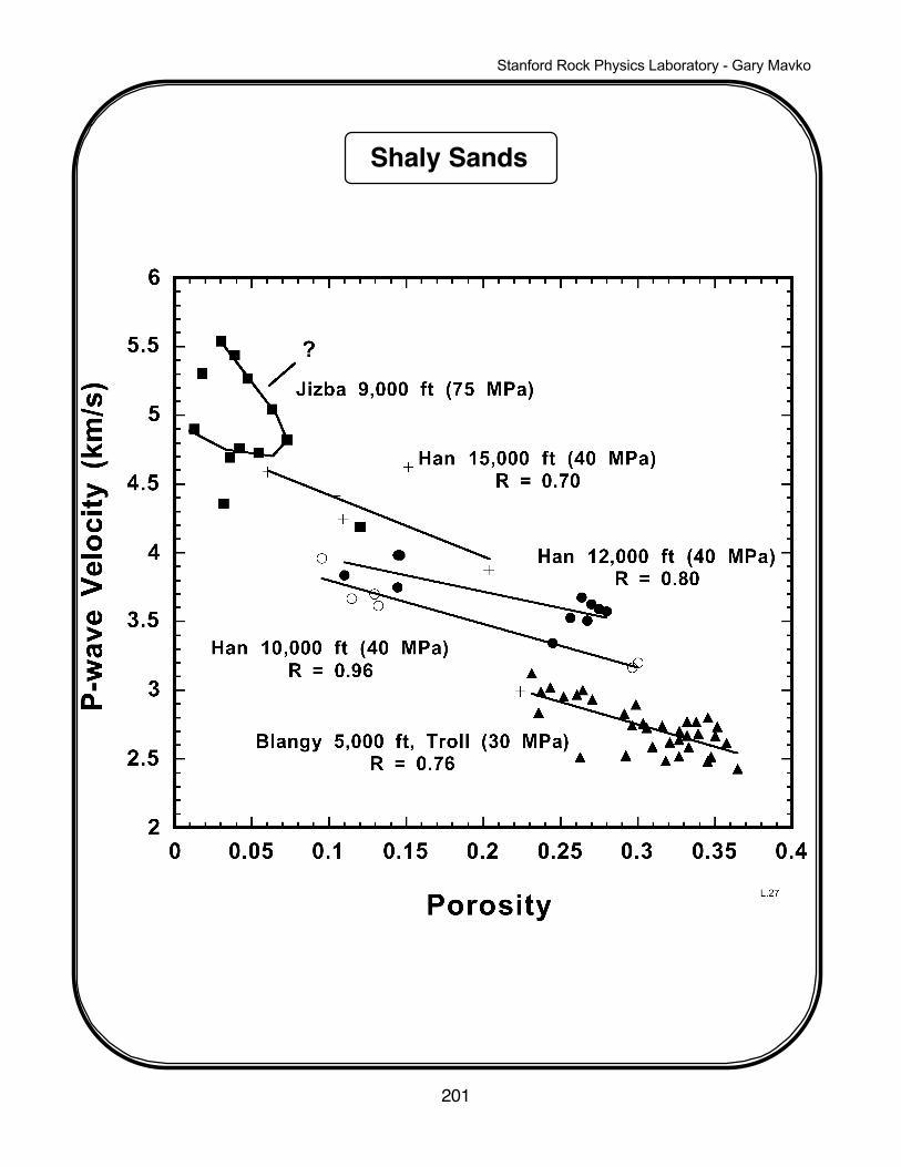
Shaly Sands
201
L.27
Stanford Rock Physics Laboratory - Gary Mavko
Shaly Sands
202
Xu and White (1995) developed a theoretical model for velocities in shaly sandstones.
the formulation uses the Kuster-Toksöz and Differential Effective Medium theories to
estimate the dry rock P and S velocities, and the low frequency saturated velocities
are obtained from Gassmann’s equation. The sand-clay mixture is modeled with
ellipsoidal inclusions of two different aspect ratios. The sand fraction has stifferpores with aspect ratio α ≈ 0.1 - 0.15, while the clay-related pores are more compliant
with α ≈ 0.02-0.05. The velocity model simulates the “V” shaped velocity-porosity
relation of Marion et al. (1992) for sand-clay mixtures. The total porosity φ = φsand +
φclay where φsand and φclay are the porosities associated with the sand and clay
fractions respectively. These are approximated by
where Vsand and Vclay denote the volumetric sand and clay content respectively.
Shale volume fromlogs may be used as an estimate of Vclay. through the log derived
shale volume includes silts, and overestimates clay content, results obtained by Xu
and White justify its use. The properties of the solid mineral mixture are estimated
by a Wyllie time average of the quartz and clay mineral velocities, and arithmetic
average of t heir densities:
where subscript 0 denotes the mineral properties. these mineral properties are
then used in the Kuster-Toksöz formulation along witht he porosity and clay
content, to calculate dry rock moduli and velocities. The limitation of small pore
concentration of the Kuster-Toksöz model is handled by incrementally adding the
pores in small steps such that the non-interaction criterion is satisfied in each
step. Gassmann’s equations are used to obtain low frequency saturated
velocities. High frequency saturated velocities are calculated by using fluid-filled
ellipsoidal inclusions in the Kuster-Toksöz model.
The model can be used to predict shear wave velocities (Xu and White, 1994).
Estimates of Vs may be obtained from known mineral matrix properties and
measured porosity and clay content, or from measured Vp and either porosity or
clay content. Su and White recommend using measurements of P-wave sonic log
since it is more reliable than estimates of shale volume and porosity.
φsand = 1 – φ – Vclay
φ1 – φ = Vsand
φ1 – φ
φclay = Vclay
φ1 – φ
1VP0
=1 – φ – Vclay
1 – φ1
VPquartz
+Vclay1 – φ
1VPclay
1VS 0
=1 – φ – Vclay
1 – φ1
VSquartz
+Vclay1 – φ
1VSclay
ρ0 =
1 – φ – Vclay1 – φ ρquartz +
Vclay1 – φρclay
Stanford Rock Physics Laboratory - Gary Mavko
Shaly Sands
203
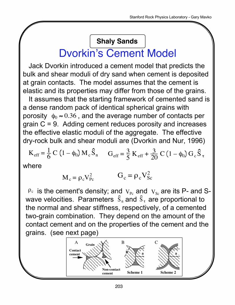
GrainContactcement
A B
R a a
Non-contactcement Scheme 1 Scheme 2
C
Dvorkin’s Cement Model
Gc = ρ cVSc2
Keff = 16 C 1 – φ0 M c Sn
M c = ρcVPc2
Geff = 35 K eff + 3
20 C 1 – φ0 G c S τ
is the cement's density; and and are its P- and S-wave velocities. Parameters and are proportional tothe normal and shear stiffness, respectively, of a cementedtwo-grain combination. They depend on the amount of thecontact cement and on the properties of the cement and thegrains. (see next page)
ρc VPc VSc S n
S τ
Jack Dvorkin introduced a cement model that predicts thebulk and shear moduli of dry sand when cement is depositedat grain contacts. The model assumes that the cement iselastic and its properties may differ from those of the grains. It assumes that the starting framework of cemented sand isa dense random pack of identical spherical grains withporosity , and the average number of contacts pergrain C = 9. Adding cement reduces porosity and increasesthe effective elastic moduli of the aggregate. The effectivedry-rock bulk and shear moduli are (Dvorkin and Nur, 1996)
where
φ0 ≈ 0.36
Stanford Rock Physics Laboratory - Gary Mavko
Shaly Sands
204
where G and are the shear modulus and the Poisson's ratio of the grains, respectively; and are the shear modulus and the Poisson's ratio of the cement; a is the radius of the contact cement layer; R is the grain radius.
Dvorkin’s Cement ModelConstants in the cement model:
S n = A n α2 + B n α + C n
A n = – 0.024153 Λ n–1.3646
Bn = 0.20405 Λ n–0.89008
Cn = 0.00024649 Λ n–1.9864
S τ = A τ α2 + B τα + C τ
A τ = –10–2 2.26ν2 + 2.07ν + 2.3 Λ τ0.079ν2 + 0.1754ν – 1.342
B τ = 0.0573ν2 + 0.0937ν + 0.202 Λ τ0.0274ν2 + 0.0529ν – 0.8765
C τ = –10–4 9.654ν2 + 4.945ν + 3.1 Λ τ0.01867ν2 + 0.4011ν – 1.8186
Λ n = 2G c
πG1 – ν 1 – ν c
1 – 2ν c
Λ τ = G c
πG α = a
R
ν νc
Gc
Stanford Rock Physics Laboratory - Gary Mavko
Shaly Sands
205
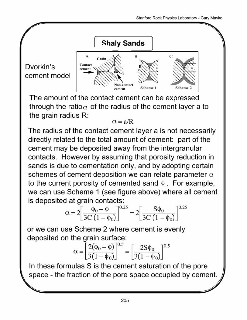
The amount of the contact cement can be expressed through the ratio of the radius of the cement layer a to the grain radius R:
α
α = a/RThe radius of the contact cement layer a is not necessarily directly related to the total amount of cement: part of the cement may be deposited away from the intergranular contacts. However by assuming that porosity reduction in sands is due to cementation only, and by adopting certain schemes of cement deposition we can relate parameter to the current porosity of cemented sand . For example, we can use Scheme 1 (see figure above) where all cement is deposited at grain contacts:
αφ
α = 2 φ0 – φ
3C 1 – φ0
0.25= 2 Sφ0
3C 1 – φ0
0.25
or we can use Scheme 2 where cement is evenlydeposited on the grain surface:
α = 2 φ0 – φ
3 1 – φ0
0.5= 2Sφ0
3 1 – φ0
0.5
In these formulas S is the cement saturation of the porespace - the fraction of the pore space occupied by cement.
Dvorkin’scement model
GrainContactcement
A B
R a a
Non-contactcement Scheme 1 Scheme 2
C
Stanford Rock Physics Laboratory - Gary Mavko
Shaly Sands
206
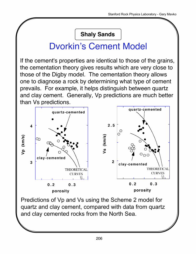
If the cement's properties are identical to those of the grains,the cementation theory gives results which are very close tothose of the Digby model. The cementation theory allowsone to diagnose a rock by determining what type of cementprevails. For example, it helps distinguish between quartzand clay cement. Generally, Vp predictions are much betterthan Vs predictions.
Predictions of Vp and Vs using the Scheme 2 model for quartz and clay cement, compared with data from quartz and clay cemented rocks from the North Sea.
Dvorkin’s Cement Model
Stanford Rock Physics Laboratory - Gary Mavko
Shaly Sands
207
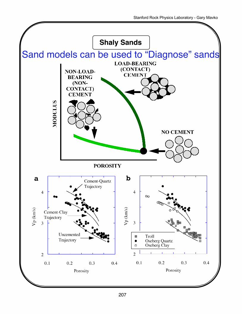
Sand models can be used to “Diagnose” sands
Stanford Rock Physics Laboratory - Gary Mavko
Shaly Sands
208
Dvorkin’s Uncemented Sand ModelThis model predicts the bulk and shear moduli of dry sandwhen cement is deposited away from grain contacts. Themodel assumes that the starting framework of uncementedsand is a dense random pack of identical spherical grainswith porosity , and the average number of contactsper grain C = 9. The contact Hertz-Mindlin theory gives thefollowing expressions for the effective bulk ( ) andshear ( ) moduli of a dry dense random pack ofidentical spherical grains subject to a hydrostatic pressureP:
φ0 = 0.36
KHM GHM
KHM = C2 1 – φ0
2 G2
18 π2 1 – ν 2 P1/3
GHM = 5 – 4ν
5 2 – ν3C2 1 – φ0
2 G 2
2π2 1 – ν 2 P1/3
where is the grain Poisson's ratio and G is the grain shear modulus.
ν
Stanford Rock Physics Laboratory - Gary Mavko
Shaly Sands
209
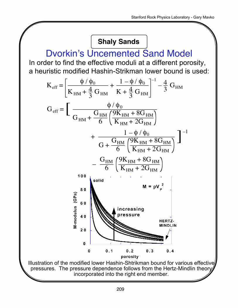
Dvorkin’s Uncemented Sand ModelIn order to find the effective moduli at a different porosity, a heuristic modified Hashin-Strikman lower bound is used:
Keff = φ / φ0
K HM + 43 G HM
+ 1 – φ / φ0
K + 43 G HM
–1– 4
3 GHM
G eff = [ φ / φ0
G HM + G HM6
9KHM + 8G HMK HM + 2GHM
+ 1 – φ / φ0
G + GHM6
9K HM + 8GHMKHM + 2GHM
]–1
– GHM6
9KHM + 8G HMKHM + 2GHM
Illustration of the modified lower Hashin-Shtrikman bound for various effectivepressures. The pressure dependence follows from the Hertz-Mindlin theory
incorporated into the right end member.
Stanford Rock Physics Laboratory - Gary Mavko
Shaly Sands
210
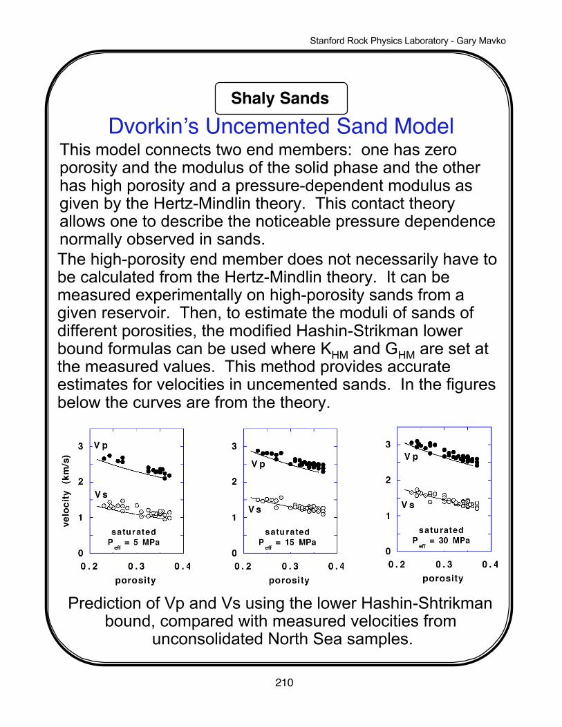
Dvorkin’s Uncemented Sand ModelThis model connects two end members: one has zeroporosity and the modulus of the solid phase and the otherhas high porosity and a pressure-dependent modulus asgiven by the Hertz-Mindlin theory. This contact theoryallows one to describe the noticeable pressure dependencenormally observed in sands.The high-porosity end member does not necessarily have tobe calculated from the Hertz-Mindlin theory. It can bemeasured experimentally on high-porosity sands from agiven reservoir. Then, to estimate the moduli of sands ofdifferent porosities, the modified Hashin-Strikman lowerbound formulas can be used where KHM and GHM are set atthe measured values. This method provides accurateestimates for velocities in uncemented sands. In the figuresbelow the curves are from the theory.
Prediction of Vp and Vs using the lower Hashin-Shtrikman bound, compared with measured velocities from
unconsolidated North Sea samples.
Stanford Rock Physics Laboratory - Gary Mavko
Shaly Sands
211
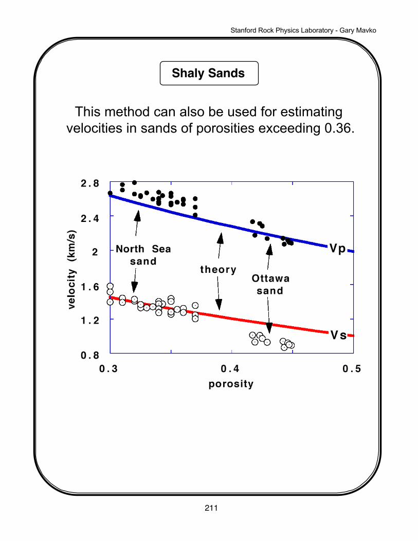
This method can also be used for estimating velocities in sands of porosities exceeding 0.36.
Stanford Rock Physics Laboratory - Gary Mavko
Shaly Sands
212
2 3
2 .1
2 .2
2 .3
Vp (km/s)
Dep
th (
km)
Well #1
A40 80 120
G RB2 3 4
1 .7
1 .8
1 .9
Vp (km/s)
Well #2
Dep
th (
km)
C
Marl
Limestone
40 80 120G RD
2 .5
3
3 .5
0.25 0 .3 0.35 0 .4
Vp
(km
/s)
Porosity
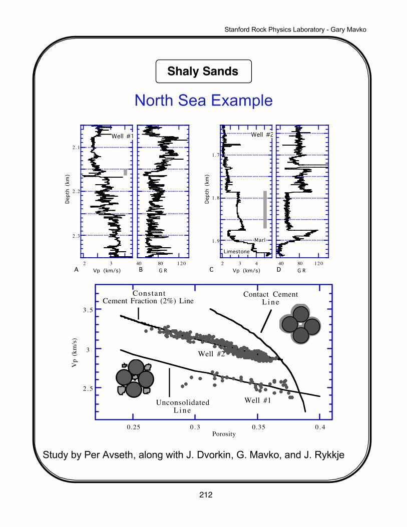
Contact CementL i n e
UnconsolidatedL i n e
ConstantCement Fraction (2%) Line
Well #1
Well #2
North Sea Example
Study by Per Avseth, along with J. Dvorkin, G. Mavko, and J. Rykkje
Stanford Rock Physics Laboratory - Gary Mavko
Shaly Sands
213
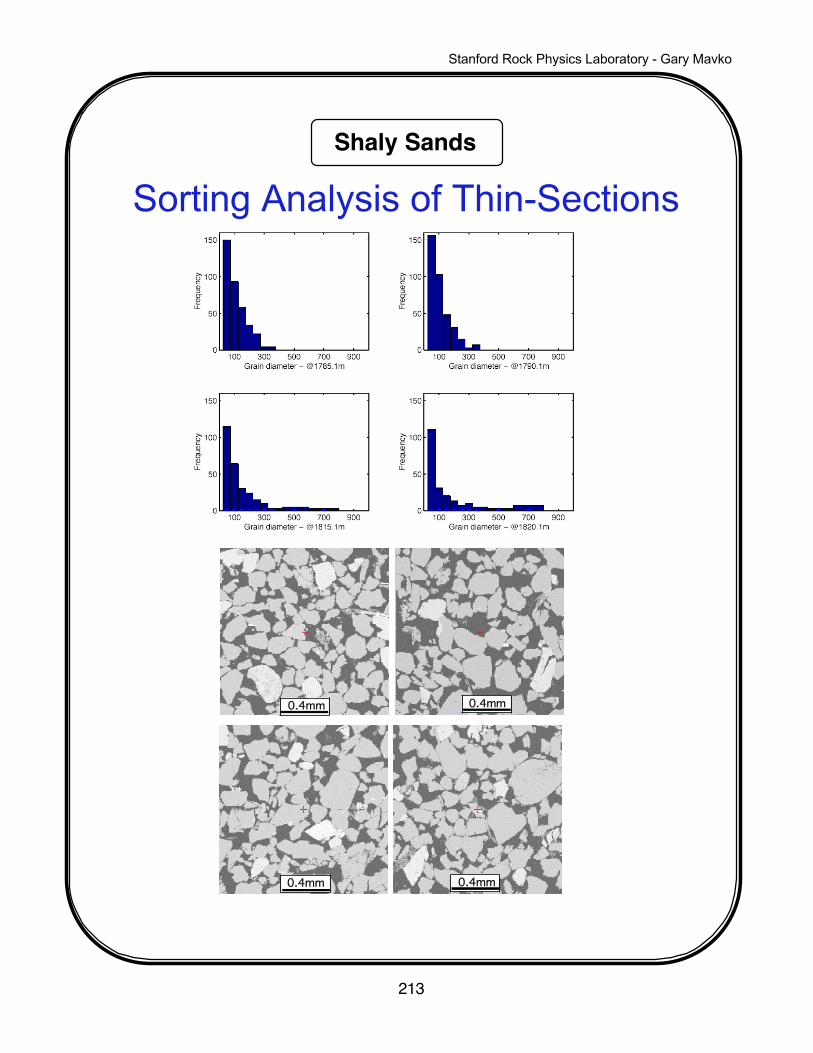
Sorting Analysis of Thin-Sections
0.4mm0.4mm
0.4mm0.4mm
Stanford Rock Physics Laboratory - Gary Mavko
Shaly Sands
214
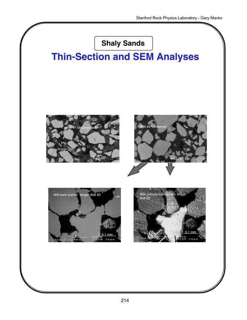
Thin-Section and SEM Analyses
Well #2 Cemented
0.25 mm
Well #1 Uncemented
0.25 mm
SEM cathode-luminescent image:Well #2
0.1 mm0.1 mm
SEM back-scatter image: Well #2
Unconsolidated
(Facies IIb)Cemented
(Facies IIa)
Back-scatter light Cathode lum. light
Qz-cement rimQz-grain


![TAR-SANDS (ARENAS BITUMINOSAS) [OIL-SANDS]](https://img.pdfslide.net/doc/110x75/546e6d60b4af9faa268b468b/tar-sands-arenas-bituminosas-oil-sands.jpg)