A091 49 AIR FORCE INST OF TECH WRIGHT-PATTERSON AFB ON F/6 15/5AANALYSIS OF AIR FORCE AVIONIC TEST STATION UTILIZATION USINB--ETC(U)

DEC 79 J R LOWELLLASSFIEDi T-I-79265TNL

7 llllllffffff

11-1111I 1 5L3

L 360

MICROCOPY RESOLUTION TEST CHART

Iq r -CI--EPOR DOUIANTA.IONPAG'0'READ) INSTRUCTIONSC, FORE ('OMPLETINC. FORM

2. ~ 0 GVHII CIPIENT'S CATALOG NUMBER

s. TYPE7 OFRPR EIDCVED

10 An -Analysis of Air Force Avionic Test St at ,i o .nTYEORPRTAEIDCVRDUtilization Using 5-Gert Modeling and Simulation. THESIS/K 6VTATAkt

6. PERFORMING ORG. REPORT NUMBER

-. 8. CONTRACT OR GRANT NUMBER()

OJmsRussell/ Lowell /

9. PERFORMING ORGANIZATION NAME AND ADDRESS 10 AREARAMWOREMUNT. NUMB A

A.FT STUDENT AT: Arizona State University

4 II. CONTROLLING OFFICE NAME AND ADDRESS.

15a. DECL ASSI FIC ATION/ DOWNGRADINGSCHEDULE

!1S. DISTRIBUTION STATEMENT (of this Report) M r -lw

APPROVED FOR PUBLIC RELEASE; DISTRIBUTION UNLIMITED E TNV1 0 1980'

SEC17. DISTRIBUTION STATEMENT (at the abstract entered in Block 20, it different Itmn Report) E

IS. SUPPLEMENTARY NOTES fih

APPROVED FOR PUBLIC RELEASE: IAW AFR 190-17 Rii C. LYN x*,.~i

25 EP 980Wright-Patterson AFB. OHl 45433St. KEY WORDS (Continue on reverse aide it necesesary end Identify by black number)

C- 20. ASRACT (Continue an reverse ide it necessary and Identify by block number)

ATTACHED

0U 1JAN7 1473 EDITION OF INO4VSS5IS OBSOLK NLSIt RITY CL. ATION OF THIS PAGIE (When 0 eat )

ABSTRACT

James Russell Lowell, M.S.E., Arizona State University, December,

1979. An Analysis of Air Force Avionic Test Station Utilization Using

Q-GERT Modeling and Simulation.

Air Force man gers must determine avionic maintenance support

resource levels pri to employment of the weapon system associated with

such support. A need xists for a method by which probable maintenance

support requirements may evaluated so that resource allocation may be

accomplished with confidence. The objective of this report is to show

that Graphical Evaluation and Review Technique with Queueing (Q-GERT)

simulation can be used to evaluate avionic maintenance support systems.

And, that simulation analysis can provide data for avionic maintenance

resource allocation.

->This report demonstrates the use of Q-GERT to: model an Air Force

avionic maintenance system; evaluate the maintenance system through simu-

lation; determine maintenance resource requirements; and, aid management

with day-to-day decisions. A Q-GERT network model is developed and trans-

lated into computer input format. Simulation of this model is accomplished

to provide data for analysis. Analysis illustrates the use of this method

as an aid to Command level and Base level decision makers.

esuts of this analysis leads to the conclusion that Q-GERT can be

used to answer critical questions concerning the availability uf avionic

maintenance support resources.

AN ANALYSIS OF AIR FORCE AVIONIC

TEST STATION UTILIZATION USING

Q-GERT MODELING AND SIMULATION

by

Jamies Russell Lowell

AN ENGINEERING REPflRT PRESENTED IN

PARTIAL FI.'FILLTIENT OF THE REQ!IIRE.IPENTS

FOR THE I)EGREE

MASTER OF SCIEMCE IN EMGINEERING

Accession For

NTIS GRiA&IDDC TAB

UnannouncedJust if icat io

Disrib~on

ARIZONA STATE UPNIVERSITY Dit Avail and/oru~t pecial

FACULTY A.V INnUST'RIAL ENGINEERING f~ ________

Decemiber 1979

TABLE OF CONTENTS

1. Introduction.............................................. 1

,1Background..............................................1IResearch Objective ....................................... 2Research Scope .......................................... 2Overview................................................ 3

II. Problem Definition ........................................ 4

Sortie Generation........................................ 4Maintenance Support...................................... 4Aircraft Systems/Subsystems............................... 5System Failure .......................................... 5Avionic Intermediate Shop ................................ 6System Modeling Requirements.............................. 7Parameters of Evaluation ................................. 9

111. Q-GERT Modeling........................................... 10

Development of Q-GEP.................................... 10Summary of Modeling and Notation.......................... 11

IV. Model of the System ....................................... 21

System Definition ....................................... 21Aircraft Generation ..................................... 22Sortie Generation and System Failure...................... 24LRIJ Failure and Repair ................................... 27Test Station Failure .................................... 31Control of Time......................................... 33

V. Model Validation.......................................... 37

V.erification of Model.................................... 37Analytic Estimation ..................................... 37Comparison Test ......................................... 39

VI. Command Level 9ecisions.................................... 42

Decision Analysis with Q-GFPT............................. 42Test Station Acquisition Relative to Sortie Requirements..45

Problems Encountered in Test Station Acquisition ..........45Development of Decision Criteria........................ 46Simulation and Regression Analysis...................... 48Decision Rule............................................... 51

Test Station Acquisition Relative to Expected Costof LRUi Repair..................................................... 55

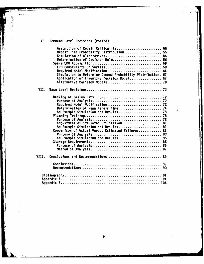
VI. Command Level Decisions (cont'd)

Assumption of Repair Criticality ........... ............ 55Repair Time Probability Distribution .................... 55Simulation of Alternatives .............................. 56Determination of Decision Rule .......................... 56

Spare LRi Acquisition ..................................... 59LR! Constraints On Sorties .............................. 59Required Model Modification ............................. 64Simulation to Determine Demand Probability Distribution. 67Application of Inventory Dec4sion Model ................. 67Alternative Decision Models ............................. 70

VII. Base Level Decisions ........................................ 72

Backlog of Failed LRUs .................................... 72Purpose of Analysis ..................................... 72Required Model Modification ............................. 72Determination of Mean Repair Time ....................... 74An Example Simulation and Results ....................... 78

Planning Training ......................................... 78Purpose of Analysis.................... ............... 78Adjustment of Simulated Utilization ..................... 81An Example Simulation and Results ....................... 81

Comparison of Actual Versus Estimated Failures ............ 83Purpose of Analysis ..................................... 83An Example Simulation and Results ....................... 85

Storage Requirements ...................................... 85Purpose of Analysis ..................................... 85Method of Analysis ...................................... 87

VIII. Conclusions and Recommendations ............................. 89

Conclusions ............................................... 89Recommendations ........................................... 90

Bibliography .................................................... 91Appendix A ...................................................... 94Appendix B ...................................................... 106

) ii

m.)

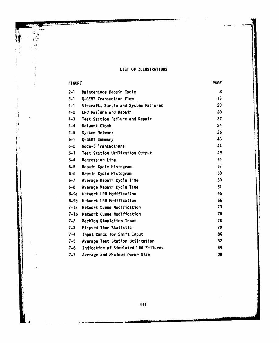
LIST OF ILLUSTRATIONS

FIGURE PAGE

2-1 Maintenance Repair Cycle 8

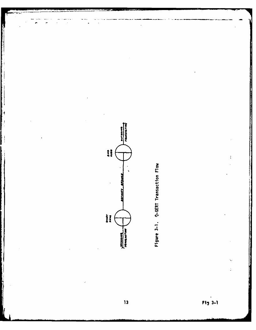
3-1 Q-GERT Transaction Flow 13

4-1 Aircraft, Sortie and System, Failures 23

4-2 LRU Failure and Repair 28

4-3 Test Station Failure and Repair 32

4-4 Network Clock 34

4-5 System Network 36

6-1 Q-GERT Summary 43

6-2 Node-5 Transactions 44

6-3 Test Station Utilization Output 49

6-4 Regression Line 54

6-5 Repair Cycle Histogram 57

6-6 Repair Cycle Histogram 58

6-7 Average Repair Cycle Time 60

6-8 Average Repair Cycle Time 61

6-9a Network LRU Modification 65

6-9b Network LRU Modification 66

7-la Network Queue Modification 73

7-lb Network Queue Modification 75

7-2 Backlog Simulation Input 76

7-3 Elapsed Time Statistic 79

7-4 Input Cards for Shift Input 80

7-5 Average Test Station Utilization 82

7-6 Indication of Simulated LR) Failures 84

7-7 Average and Maximum Queue Size 38

ii'

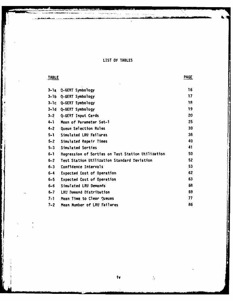
LIST OF TABLES

TABLE PAGE

3-la Q-GERT Symbology 16

3-lb Q-GERT Symbology 17

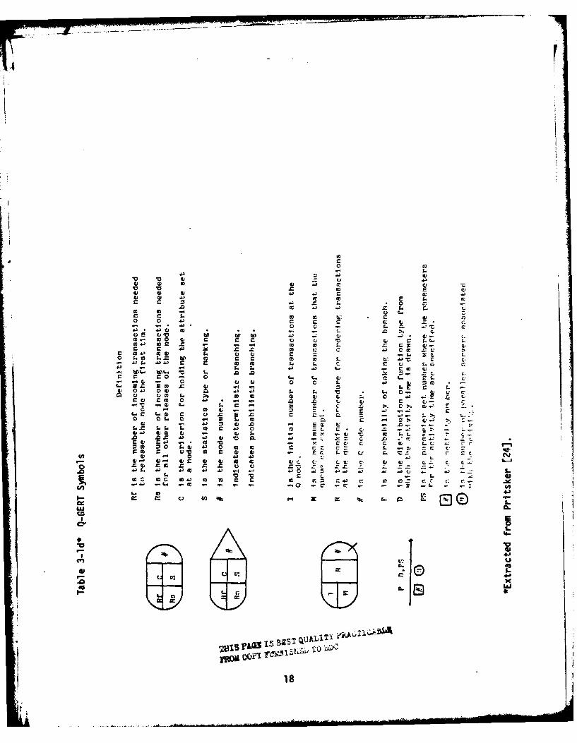
3-1c Q-GERT Symbology 18

3-id Q-GERT Symbology 19

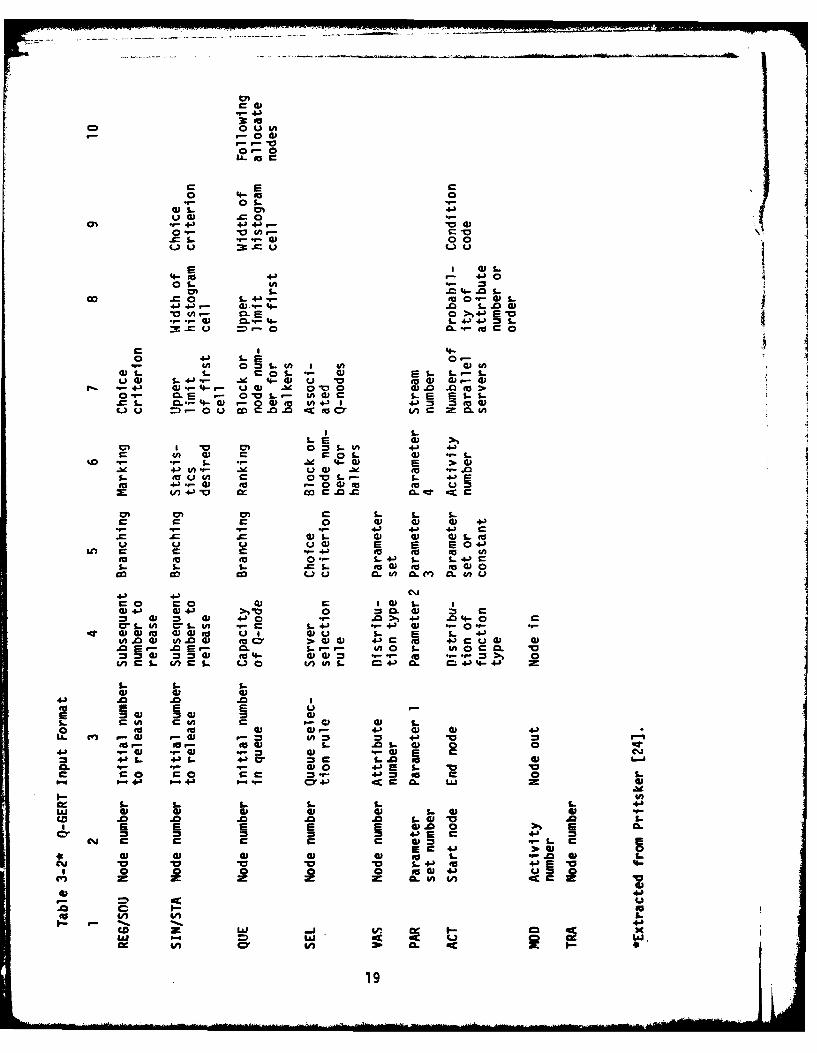
3-2 Q-GERT Input Cards 20

4-1 Mean of Parameter Set-i 25

4-2 Queue Selection Rules 30

5-1 Simulated LRU Failures 38

5-2 Simulated Repair Times 40

5-3 Simulated Sorties 41

6-1 Regression of Sorties on Test Station Utilization 50

6-2 Test Station Utilization Standard Deviation 52

6-3 Confidence Intervals 53

6-4 Expected Cost of Operation 62

6-5 Expected Cost of Operation 63

6-6 Simulated LRU Demands 68

6-7 LRU Demand Distribution 69

7-1 Mean Time to Clear Queues 77

7-2 Mean Number of LRU Failures 86

ivi

Ij!

I. INTRODUCTION

Assessment of resource requirements and costs associated with the

support of flying activities in various United States Air Force (USAF)

organizations is a continuing problem. As new aircraft systems and

subsystems enter the inventory, there exists a recurring need for

reliable estimates of maintenance resource requirements to activate,

maintain, and deploy the emerging system. Such estimates aid USAF

managers in allocating maintenance resources to insure mission capa-

bility in a timely manner [8].

Background

A method presently used for such evaluations is the Logistics

Composite Model (LCOM) simulation technique. With the LCOM simulation

language, USAF base level aircraft maintenance and support activities

are modeled [10, 11]. Simulation with such a model has been used

successfully to determine maintenance manpower requirements to support

specified levels of flying activities for several tactical weapon

systems (4).

Air Force Test and Evaluation Center (AFTEC) analysis using LCOM

has extended the use of LCOM to include assessment of the sensitivity

of sortie generation capability to: manpower; spare parts and support

equipment levels; reliability/maintainability parameters; and Avionic

Intermediate Shop (AIS) test station availability. Although successful,

I-Now -

because of the complexity of LCOM, modeling and analysis of AIS becomes

very time consuming and expensive. Consequently, AFTFC has suggested

a research effort to develop a procedure by which the Queueing Graph-

ical Evaluation and Review Technique (Q-GERT) may be used for AIS

sensitivity analysis [23]. Use of Q-GERT is suggested since its appli-

cation and simplistic approach will enable more timely and cost effective

analysis that will interface well with other ongoing simulation efforts

such as LCOM.

Research Problem

A need exists to analyze critical questions concerning test station

availability and the effects of that availability on sortie generation

capability. AFTEC has suggested the use of Q-GERT as the modeling tool

to conduct such analysis [3).

qesearch Objective

In this research project, the author will use Q-GERT to model and

analyze the F-16 AIS. The modeling effort includes identification and

definition of the system and system parameters and translation of such

parameters into Q-GERT networks. With a basic model constructed, simu-

lation is accomplished and analysis of simulation results is discussed.

Research Scope

The intent of this report is to describe Q-GERT model development

and analysis procedures applicaable to USAF weapon system support

2

evaluation. The F-16 weapon system is used as an example of the appli-

cation. Although data parameters are realistic, they are not assumed

to be accurate. Sortie rate requirements herein are completely ficti-

cious and should not be used for USAF analysis.

Overview

The remainder of this report consists of seven chapters. The

Problem Definition chapter describes the system to be simulated and

the type of evaluation required. The Q-GERT chapter provides the

reader with the Q-GERT network and analysis concepts necessary for the

reading of this report. The Modeling chapter details the process by

which the defined system is translated into the Q-GEPT simulation

language. In the Model Validation, Command Level Decision, and Base

Level necisions chapters, discussion of simulation output and the

analysis of that output is presented. Finally, the Conclusions and

Recommendation chapter summarizes the research findings.

IIk.3

II. PROBLEM PEFINITION

This chapter contains a description of the maintenance system to

be modeled. It also identifies and defines evaluation requirements

and the parameters used in the evaluation. The description includes

pertinent assumptions and the maintenance process.

Sortie Generation

Within the USAF, the flight of an aircraft is termed a sortie.

When an aircraft takes off, flys some maneuver, and lands, one sortie

is constituted. Many support resources are measured in terms of this

sortie since plans are based on how many sorties are required by each

aircraft per day to accomplish a desired goal [1, 3]. Sortie require-

ments of this report are fictitious and should not be considered in

any F-16 analysis.

Maintenance Support

Sortie generation is mainly a function of aircraft availability.

It is obvious that an aircraft which is unavailable cannot fly, and

an aircraft in repair status is considered unavailable. Maintenance

support is designed to process aircraft repair in an expedient manner

to assure availability. This maintenance is usually accomplished by

removing a failed component from an aircraft system and replacing it

with a good like item from supply stock. The aircraft is then available

4

for sortie generation while the failed component is repaired in a

maintenance shop.

Aircraft Systems/Subsys tems

For purposes of maintenance support, aircraft within the LISAF

are subdivided into systems. Each system such as Engines, Fuels,

and RADAR has specialists trained specifically as maintenanace tech-

nicians. Within a system, sybsystems such as Navigational RAPAR and

Fire Control RADAR exist. These sybsystems are made up of functional

component "black boxes" such as computers, control units, transmitters,

receivers, etc. Each of these component"black boxes" is referred to

as a line replaceable unit (LRU) and constitute the components that

are removed and replaced on the aircraft and repaired in the main-

tenance shop.

Aircraft System Failure

Each system on an aircraft is subject to failure. The Air Force

measures these system failures in terms of number of sorties flown.

Systems have a failure parameter, assumed to he exponentially distri-

buted, of Mean Sortie Between Maintenance Action (MSBVA) [27]. When

an aircraft system fails, one of two methods of aircraft repair occurs.

The first of these methods involves the removal of an LRU, the second

method does not. Empirical data provides estimates for the probability

of LRU removal, given failure of the parent system, for most weapon

systems. When a new weapon system with no empirical data is studied,

5

' .

a comparability study is conducted to extrapolate date from one weapon

system to another [27].

Avionic Intermediate Shop

Electronic components of avionic systems, removed from an aircraft,

are processed through Avionic Intermediate Shops (AIS) for repair.

Modern weapon system AIS rely on an Automatic Test Set with specific

test stations designed for functional repair of avionic components.

Upon removal from an aircraft, a given LRU will enter the shop and

either go directly to the test station that has repair capability for

the unit or it will be placed in waiting status for the availability of

the test station. Each test station has the capability to perform diag-

nostic and fault isolation for several LRI~s within a functional group.

Systems such as these usually have some sort of adaptors designed to

interface the LRU with the test station. Connecting the LRU and inter-

face adaptor to the test station constitutesa set-up procedure.

When a LRU is assigned to a test station there are three basic

types of maintenance actions that may be taken; bench check and repair;

bench check and no repair required; and not repairable this station [3).

There is an expected task time associated with each of the repair

actions that the Air Force has determined to be Lognormally distributed

[15). Upon completion of either repair or no repair required actions,

the LRU is returned to supply stock to be used on an aircraft as required.

If the LRU is not repairable, it is shipped off-base to a depot repair

6

facility. This unit is lost to the base supply system until replenish-

ment occurs.

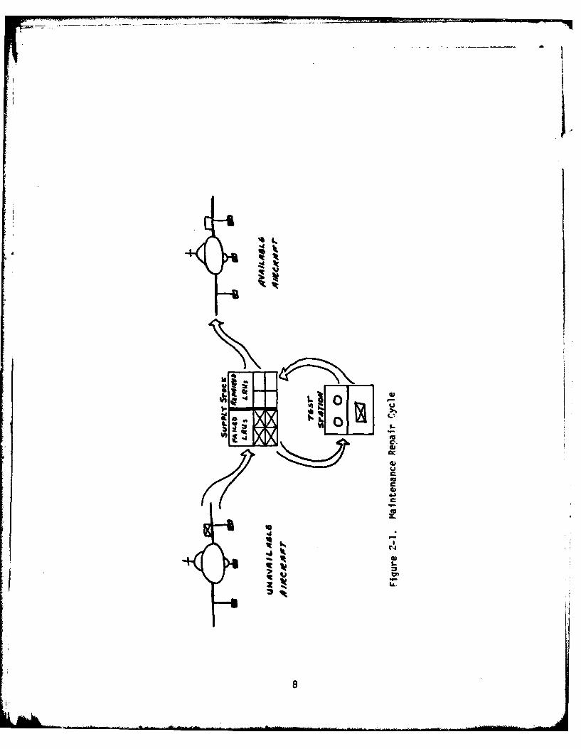
System Modeling Requirements

The object of this research is the analysis of AIS test stations

and the effects they have on sortie generation. The following overview,

in conjunction with the figure 2-1, details the maintenenace system of

interest.

A predetermined sortie generation requirement drives avionic system

failures based on MSBMA. When a given system fails, the type of organi-

zational maintenance required on the aircraft is determined probabilist-

ically. If a remove action is required and a LRU spare is available

for replacement, the aircraft returns to available status and the failed

LRU is routed to the shop. If there is no spare LR!, the LRU removed

from the aircraft must be repaired and reinstalled prior to the aircraft

becoming available for flight.

A LRU removed from the aircraft is transported to the shop and may

either enter awaiting maintenance (AWM) status or go directly to the

appropriate test station depending on test station availability. When

the test station is available, the LRU repair action is determined prob-

abilistically with the time to repair selected from a Lognormal distri-

bution. The LRU repair action may lead to replenishment of supply stock,

repair of an aircraft, or a depot delay depending on the predetermined

type of removal for the aircraft or the probabilistic repair action

taken.

7

t

-.-

viu

I

it

L.

&MML

Parameters of Evaluation

Analysis of this system requires that control over attempted or

scheduled sorties is available to the analyst. There must also be a

method to allow failures based on MSBMA and the probabilities associ-

ated with LRU removal given a system failure.

With a LRU flow into the shop initiated, it is necsssary to

follow each LRU through the shop process to determine the average

total time in the shop, average time in queues, and total number pro-

cessed. The cumulation of these repair activities will provide a test

station utilization statistic.

Iterative simulation over a spectrum of sortie generation rates

and the above mentioned statistics will provide the necessary data to

determine test station resources required to support given sortie

generation rates.

! 1E9

III. Q-GERT MOnELING

Development of Q-GERT

The technique used herein is an extension of the GERT simulation

models, and GERT model development will be duscussed to summarize the

events which lead to Q-GERT. For the reader interested in a detailed

treatment, refer to T24, 25, 26].

GERTis a result of an extension of the modeling capabilities of

PERT and CPM. Pritsker and Happ [26] developed and defined this

* "stochastic network" or Graphical Evaluation and Review Technique

(GERT) network. Generally, stochastic networks are characterized by:

1. Directed branches representing activities or processes,

2. Each branch is assigned a probability of occurrence and other

parameters which describe the distribution of time to traverse the

branch,

3. Logical nodes which denote the precedence relationship between

the incident and emanating branches of the node, and

4. A realization of the network Is a set of branches and nodes

which define a path through the network for one experiment [16].

The input at each node may be singular or multiple with AND-type (all

incident branches must be realized) or OR-type (only one incident branch

must be realized) logic. Logic such as these allow the node to be

realized and upon realization of a node, transaction output may be

either determfnistric or probabilistic. Determine output causes the

10

release of all branches emanating from a node while probabilistic

implies that only one branch is released according to the probabilities

of the branch. Such probabilistic selection of branches emanating from

a node is mutually exclusive and the sum of probabilities must be unity.

The expanded network logic of GERT allows for network modeling

where not all of the paths of the network must be traversed to reach

the terminal point. Because of this model enhancement, GERT can be

used to model situations where one of many paths will lead to success.

'pon realization of the limitation of GERT as an analytic model,

Pritsker developed a simulator called GERTS [25]. This original simu-

lator has been revised several times and each time additional capabili-

ties and improvements in methods of data storage were added [16].

The most recent addition to the GERT family is Q-GERT. The Q

implies a capability to formulate queues at nodes designed as Q-nodes.

This feature of the model is not new; previous GERT models, particularly

GERTS-IIIQ and GERTS QR, had the same capability. The characteristics

of Q-GERT that makes it an improved model are that it combines most of

the features of all predecessor GERTS models and in addition gives the

analyst the flexibility to write and insert "user functions" which follow

the general logic of the Fortrai. based GASP IV simulation language [2].

Summary of Modeling and Notation

The first step in modeling with Q-GERT is drawing a network design

of the system to be studied. The graphical model associated with

i1

If

Q-GERT is basically a means of communicating the process of interest.

It also represents the organization and definition of the problem for

input to the computer program. Networks establish a means by which

the analyst can clearly define the relationship among system components,

the parameters of the system, and the decision points and rules within

the system. When the network is complete, the analyst may study it and

determine, in many cases without the aid of the computer, errors in

logic, or flaws in the design of the system. After concluding the

network represents the desired system, network notation is readily

transformed to computer input form. Experience has shown the network

to be an excellent means of explaining the sytem, system parameters

and impending analysis of the output to those not well versed in the

methods of Operations Research or Systems Analysis.

The network consists of branches representing activities or direc-

tional flow paths and nodes representing logical relationships between

activities. Transactions representing entities being processed, flow

through the network from node to node throuqh the branches as shown

in figure 3-1. Each branch has a starting and ending node and trans-

actions that traverse the branch are delayed by the time associated

with the activity the branch represents [24, 25]. The times associ-

ated with the activity may be selected from several built-in distri-

butions or by a user defined distribution. Each transaction may be

assigned attributes that distinguish some characteristic of the entity

being modeled. For some node-branch relationships, a transaction's

attributes can be used to identify activity parameters or branching

12

-di

-" ........- --- .- --- --... .... ... .... ... . . a- ... .. _.- -

j I!

-*1l

L

13 Ft9 3-f .k ..... .. ... .. .... ... .. .. ....... ... .... ... . ... ..... ...... . . .. .., ... ...

rules. When a transaction reaches a node, the node-type determines

disposition of that transaction. Regular nodes are used for deter-

ministic and probabilistic routing. These nodes may also invoke

conditional branching, a new feature of Q-GERT. Queue nodes detain

or hold a transaction until availability of a service facility,

resource, or match criteria release the node. New features of the

Q-GERT model that are associated with queue nodes include: select

nodes which allow the analyst to define prioritized selection and

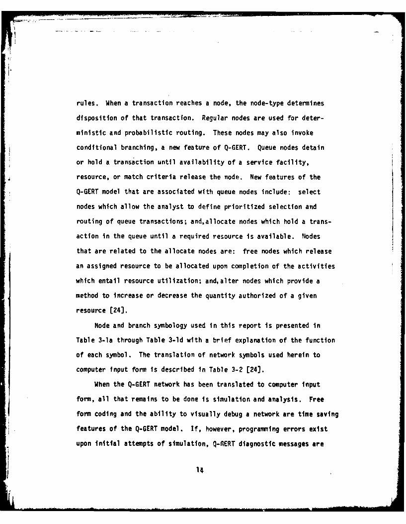
routing of queue transactions; andallocate nodes which hold a trans-

action in the queue until a required resource is available. Nodes

that are related to the allocate nodes are: free nodes which release

an assigned resource to be allocated upon completion of the activities

which entail resource utilization; and, alter nodes which provide a

method to increase or decrease the quantity authorized of a given

resource [24].

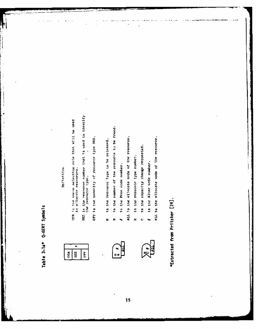
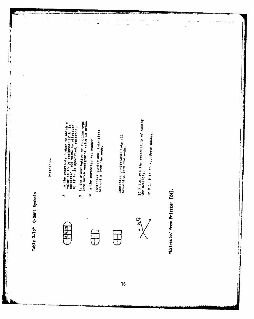
Node and branch symbology used In this report is presented in

Table 3-la through Table 3-ld with a brief explanation of the function

of each symbol. The translation of network symbols used herein to

computer input form is described in Table 3-2 [24].

When the Q-GERT network has been translated to computer input

form, all that remains to be done Is simulation and analysis. Free

form coding and the ability to visually debug a network are time saving

features of the Q-GERT model. If, however, programming errors exist

upon initial attempts of simulation, Q-GERT diagnostic messages are

14

0) 4

41 4) 4)

- 4)

4, 4: 4,C

IL L 4: C.(

C 0 .0go5. (z 0 E

IC w~ 4,

im Z4-; 414 5i 41 41 V Lv41. C . ~ 4' 0 .

-c C-

O. M,~ 4 ~ ~ C , C ~ 4CC) 4'..- : U 1.) U 4) 4

4AJ

15

0

W. 4) t ..

c a - - C - 0) aa E)4 4) .

06 c. 0 41

q 4. 4J _ ., 0 -S. O

Vj "

.q 1 . 4 A4 r 4r 0 0

U is-

.05J..~. 41 0 01

1-116

1~to

E v v00-' 0

a

4)~

t 0, cc 0)0~ 0.

0 N~ -

**Cf* 41 ~ d) suG)

0 v ca ,

*j w) P, 9.4

0)0

'~' V 0)C4v

a,~~ atJ.0

C)4J 4J

CLJ

9.-7

4-,jk

41090

4) 0) .- ,S4) x 4)- u

0 V F. =1 - C4 4 Co 4) :h C 4

V v bp 4) .0 40 * 0.0~ ~ cd 4) 4 . ..

Go 0 L.c C C m .41 9. V v -;. 3

L. . = ) 0p CI c 5 . C..-

41.$- 410 4) C E C m c C) C 5

W- C 4 A;0.04 r-C 41) 44 . C UC.5 4

41 0 .6. 41 cr . ) 1 C.v 0e4 .- 0 S, L)0 0 5 )

c- c. 24 0 4.3 . .1 C 5

4) 41 4 4) 4; 5. V * cc.

n4 0 S. 0 4) r0 z0 rC 1Cso ... 4 CS . C, -lit ' -

41 41 ) -4 41* 5 2 ~ .o.. C4 C . to .0 E r_ VC 4j - ' 4

4)4 %t4 4)J4 - 1 5I0 u00 4 ) 4 . 4 0 -4 ~ .

~~4)~~ 24101V- ~ C C C 4 -.41 ~ 5.4 4) 41 1 C 45.)CU C UV C ' * c~ -0 ~ C. V~r~.

41 - 0 4) 44)f 1~. 4)C 4) ) 4 41 )5. 52 54) 2 4 4) ).. C

o .4) 0 3 . 0 . C) )- 0) .. 0 . 0 .. 0

I,. 4 )1 4 ) . ) .~ ). 4 - 40 - 4

5..~~S V V4- . 5 -410 ~ ~ ~ ~ ~ ~ 1 BE51) 4 1 C 1 r~0) t- 4 10 r

181

3 to~ OL w

4 - m

0 'I-.

alL 0

O'h.94.ai) 00

4C- *- +) 0-)00

0 ' L.4

ao I L.- 0- a) S0

C I '4-04-) S-5 0-

4?- CA (AL I in W)inOL. L. CCS- 0 E- SL- s-LIG L4J -- -le 4-0 4) V 450 to a a)

P -4.) W -~4- U ( -hel 00 0V 01.0 .0 to>000 0. - S-- inI A Sr-S E L. -I I4L0-.4- a) -0W iCO #A4- 4J 1 9 va)i

(l)u )r-OLI o C.D.0 -cc o ' (A C 2!: CL

S- 01 4Ja) c 'O Si . .

s.D *. *- %- M a 4-) 5 >0Nd 4-)ir (Ae LI .Nd 45 a) Nd a

Ln 4-L)i C0 OVm C. c-

r- 4.)-0 4-5 e-0014 c5

a) C. a) a)0 0) . m

to- to- 4. S) 4-. L 4-) Cc .c c S- 01 03 ic 0oL45

4-) +I) II 0 -

=5 0) 4-) .0 S i- S-) 04-' 0Iin cls in +)S - 3 is "5010

4. o ) W oN 5 . 4CO CO (v C. 101 S-r>W4 4 G 4) U

034E.r .04. E S V 0 S-. 0 c CL=Si = C'v = = ) *C 4-4- .e). w3 =*to=-

Llr 0115004 LII uLc S- 5nC . m+ m =+4-44

4J5.m .05. .0. u. n . iO O: 3 45, W01 a)- 45 '9- >£fCS- CflC- CO iln 4)0 )-.

0) 01 010) )4

LCU Cin CA .0 4-) Mzto do S. 03 L' 4' v 01 0

4J. "- iW -- ap- zn 4.) "-W r V45 . 45 . 4501 S-= .0 to W

a c 0 v0 =1 to03 c4L 4- 4'rC +) c iL 01LU

0. 9- -9- 9 010 4.J5 . V

0r 1 41 E1 M1 014J1

4.) C 4.)

03 ~ ~ 01L . 'v-.0NY V v V a v L. 4-) #0 4 V'4

1 0 0 0 0 M W343 QRY ZL CA ti ac ~ c a

.01r- 43

Lai Z LAD ...J

19)

printed in the output to aid in sumulation debugging. If debugging

cannot be accomplished with the aid of these diagnostics, there is

a feature of the model that allows nodal and/or event tracing to help

locate faulty network logic.

20

IV. MODEL OF THE SYSTEM

System Definition

The system modeled is similar to the job-shop consisting of a

single homogeneous resource. Other resources are considered as always

available when the one defined resource is available. There are six

types of arrivals (LRUs),each having a Poisson arrival rate modified

by a conditional probability [27). Each arriving LRU transaction

enters a queue specified by the type LRU identified by attributes, and

no balking occurs. When a test station resource Is available, it is

allocated to one of the waiting LRU transactions allowing the LRU trans-

action to continue processing through the repair shop. Each LRU has an

exclusive set of service channels with probabilistic routing to repair

activities with mean repair times drawn from a Lognormal distribution

[15]. As each LPU completes the service activity, the test station

resource is freed and made available to be allocated to the next waiting

transaction. The completed transaction is routed to a node used as a

counter that will fail the test station after a given number of trans-

actions have been processed.

Prior to the shop process described above, an integral portion of

the system must be modeled. The arriving LRU transactions represent

failed aircraft components with failure rates based on the number of times

an aircraft has flown. Thus, the first part of the system must simulate

the generation of aircraft and the use of those aircraft to fly sorties

to drive system and LRU failures.

21

I

Additionally, the total system must include a method to control

the amount of time each day that flight and maintenance operations are

accomplished and control the number of operating days each week.

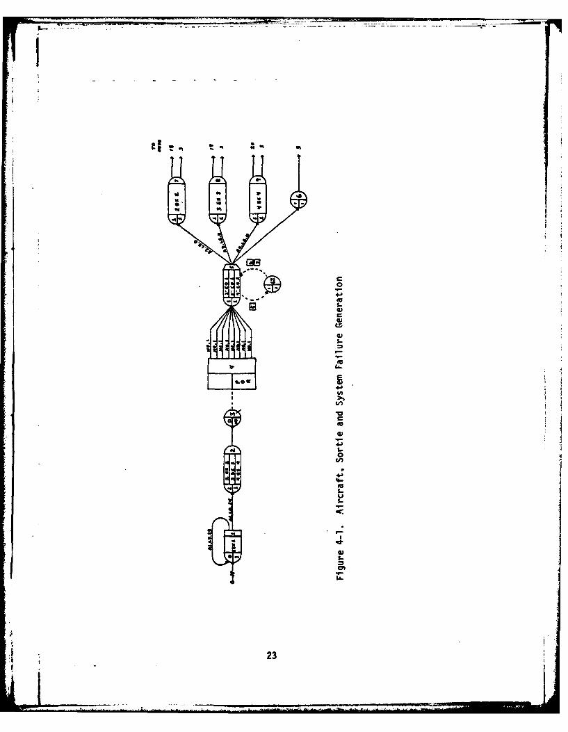
Aircraft Generation

Aircraft are generated by the source node. Each aircraft generated

is an entity which must have attributes representing avionic systems

and all aircraft entering the system will stay in the system. The

analyst must decide how many aircraft should be generated to establish

flying and failure rates. Most fighter aircraft units have flying

squadrons with 24 aircraft assigned [3, 4]. Based upon this knowledge,

the example described in this report has 24 aircraft generationed as

indicated in figure 4-1.

Source node-I is realized upon activation of the simulator and the

first transaction generated is assigned the value one, to attribute-l.

This transaction, due to the conditional take-all branching of the source

node, will traverse both paths emanating from the node. As shown, the

upper path from node-I to node-I has the condition Al.LE.23, which allows

transactions with the value of attribute-l, of 23 or less, to traverse

the path. Since node-I is also an increment node, each transaction that

causes node realization will have the value of attribute-l, increased

by one. When the value of attribute-I reaches 24, that number of air-

craft has been generated since very transaction has also traversed the

branch leading to node-2 with condition Al.LE.24.

22

r - - . - - - -

U~ WI

WI .8U U U*3 S - -

#4 Ph

..

4

96I.. -~0

C

2-- .~e. Eu

8 LCa,

a,1-

'U

.9-

EuLI.

3.0k4~)In

4~)

WI -~

0 CLu

4)I'd I..o

I In* *9

U 4.)* Ge-

'9-UI.

.9-

I-

i Eu.

a,S.

.9-U-

9,

23t . -

As each aircraft transaction generated realizes node-2, values

are assigned attributes-2,3, and 4 which indicate the number of sorties

to failure of aircraft avionic systems 41BOO, 74B00, and 74E00 respec-

tively. The values assigned these attributes are draws from Exponential

distributions with means corresponding to system MSBMA [27, 29].

Sortie Generation and System Failure

After the assignment of attributes for system failures, the trans-

action enters Q node-3, an available aircraft pool. Aircraft wait in

the available pool until selected by S node-4 to fly a sortie. As

shown in figure 4-1, the select node has eight activity branches ema-

nating from it that represent sortie selection. The activities them-

selves do not constitute a sortie but rather establish a means by

which the number of sorties flown each day can be regulated. Control

of the number of sorties is realized by changing the mean of parameter

set-1. Each of the eight activities emanating from S node-4 draws

from the distribution defined by parameter set-l to determine the delay

time for transactions traversing the network from Q node-3 to R node-5,

the sortie node. Table 4-1 lists several sortie rates that may be

desired and the corresponding mean value for parameter set-1. For

sortie rates not listed, the calculation performed to arrive at the

proper setting of the mean of parameter set-1 is:

Tu U 1

where, Tu is the mean of parameter set-l,Sn is the number of sorties desired daily,Sb is the number of branches emanating from S-node-4,

and FE is the flying envelop or number of hours of flightoperations each day.

24

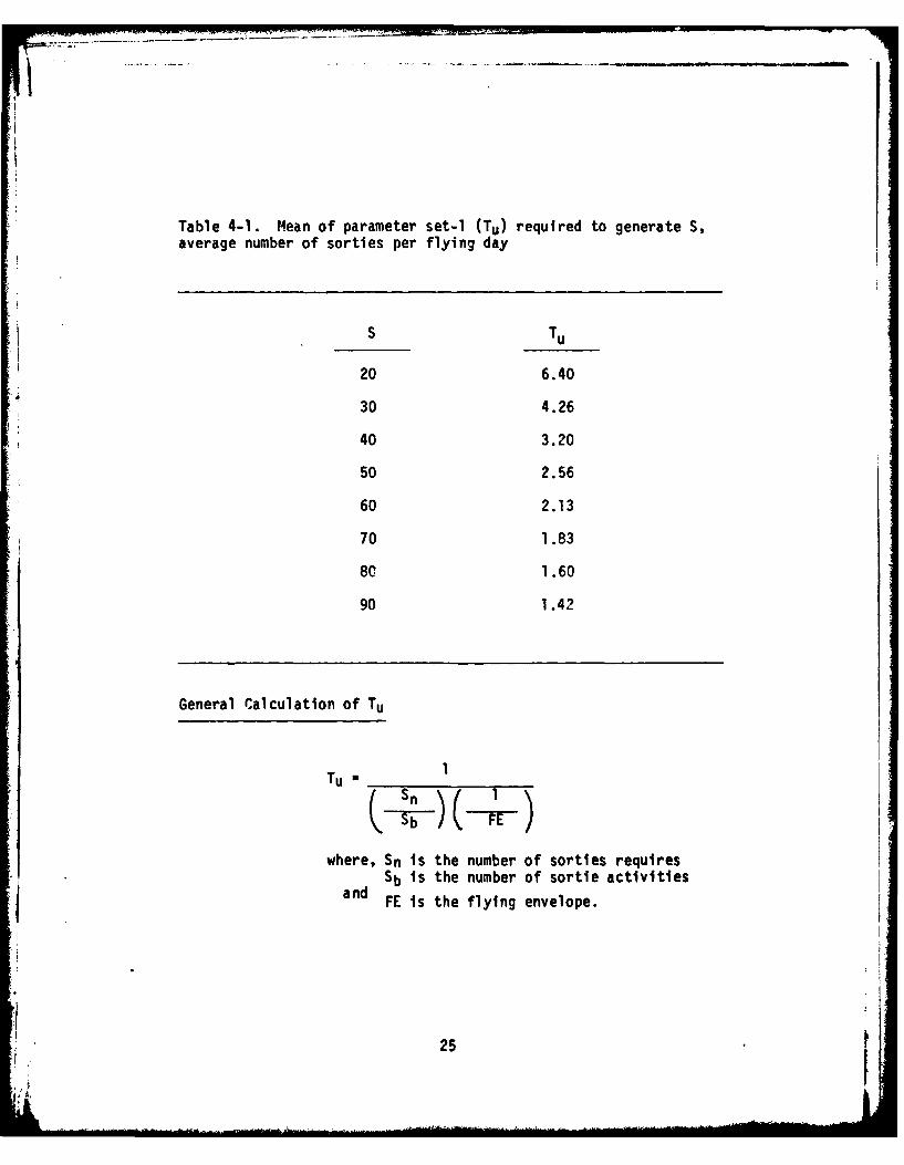
Table 4-1. Mean of parameter set-1 (Tu) required to generate S,average number of sorties per flying day

S Tu

20 6.40

30 4.26

40 3.20

50 2.56

60 2.13

70 1.83

80 1.60

90 1.42

General Calculation of Tu

Tu =

where, Sn is the number of sorties requiresSb is the number of sortie activities

and FE is the flying envelope.

25

Node-5 is a regular node with conditional take-first branching

and is the node that signifies completion of a sortie. When a trans-

action causes this node to be realized, attributes 2, 3 and 4 have

one sortie decremented from the existing attribute value. If any

attribute value is decremented to zero or less, the transaction tra-

verses the appropriate branch according to the conditions of the

branches and will cause realization of either R node-7, 8, or 9 to

indicate a system failure. As R node-7, 8, or 9 is realized indicating

system failure, the attribute for the failed system has its value

reset by another draw from the system MSBMA parameter set. Branching

from these reset nodes is deterministic thus two transactions are

emitted upon node passage. One transaction, the aircraft, returns to

the available pool while the other transaction traverses a path to a

mark node with probabilistic branching that determines LRI! failures.

If none of the attribute values are decremented to zero or less,

the transaction is routed through R node-6 to return to the available

aircraft pool.

R node-62 is part of the network that establishes control over

the periods of operation and will be discussed later.

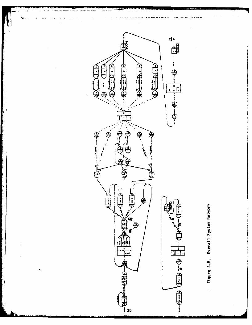
The portion of the network discussed in the previous paragraphs

and illustrated by figure 4-1 can be thought of as those events exogenous

to the shop operation discussed next. Figure 4-5 combines this portion

with all other network sections and provides a complete representation

of the system network.

26

LA

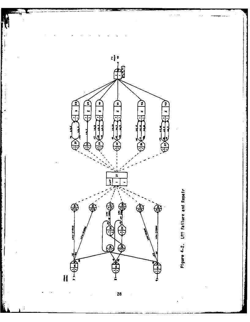
LRU Failure and Repair

The portion of the system network to be discussed next refers to

the network design of figure 4-2. This network section may be thought

of as the avionicsmaintenance shop. System failures are indicated

through realization of R nodes-18, 19, and 20. Each of these nodes

has probabilistic branching based upon the probability of a particular

LRU failure, given the system has failed. These conditional failure

probabilities are based upon Air Force empirical data as described by

Tetmeyer [27).

The probabilistic branches emanating from R nodes-18, 19, and 20

represent either the removal of a specific LRII from the aircraft or

repair of the failed system without removal of a LRU. The branching

from R node-19 illustrates a special case where historical data indi-

cates that a representative number of failures of the system produce

removal of more than one failed LRU. Each of these nodes has a path

to R node-21, which is a dead end node that absorbs all transactions

that result in no LRU removal. All other branching from these nodes

are paths by which failed LRUs reach queues to await the availability

of a test station. As mentioned in the previous section, R nodes-18,

19, and 20 also act as mark nodes that update each transaction's mark

time to current simulation time thus providing a statistic by which

the time spent in the shop for each LRU may be measured.

There are six Q nodes each representing the waiting time of a

specific LRU type for allocation of a test station resource. Q nodes

27

.1.

- .- *~ I - -S..- ~ I -.

5% 5 *~ I - -

I -- %*5% I -

%sI -

- F I- - , ' %S%% L

- * -5. % -

- - I S- - I 5. 5

F 5. 5%

a S

.3 .3 *1 0 C

i *3 . 'U

U

* p

m *~

-I

N

a

2

*1~

28

25 through 30 are the LRU queues and because any LRU that fails must

be repaired, there is no balking.

Allocate node, A node-31, allocates the test station resource to

transactions as they arrive at the queues as long as there is a free

resource. When the resource is not available, transactions must wait

in the queues until the resource is freed. Queue Selection Rules of

table 4-2 are used to control the method by which test stations are

allocated when there is competition between queues for service. In

the network of figure 4-2, the LR' that has been waiting the longest

is selected for allocation, independent of queue membership.

When allocation of a test station for a particular LRU occurs,

that LRIJ traverses a path to one of the R nodes 32 through 37 dependent

upon the queue from which the transaction emanated. Each of the R

nodes 32 through 37 with the exception of R node-33, has probabilistic

branching that determines the type repair action to be completed. LRU

repair belongs to one of three categories: bench check and repair;

bench check and no repair required; and not repairable this station.

Each of these repair actions for each LRU has a specific mean repair

time drawn from a Lognormal distribution with the variance set at

twenty-nine percent of the mean value, as described by Gunkel [15).

Upon completion of the repair activity, a statistic node is realized

which collects time statistics so that the mean time in the system for

each LRU type is included in the simulation output. Modes 38 through

43 are such statistics nodes. Transactions realizing nodes 38 through

29

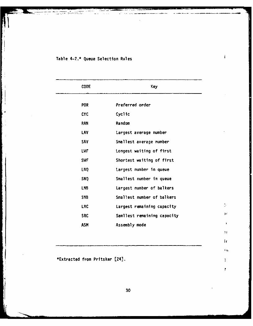
Table 4-2.* Queue Selection Rules

CODE Key

POR Preferred order

CYC Cyclic

RAN Random

LAY Largest average number

SAV Smallest average number

LWF Longest waiting of first

SWF Shortest waiting of first

LNQ Largest number in queue

SNQ Smallest number in queue

LNB Largest number of balkers

SNB Smallest number of balkers

LRC Largest remaining capacity

SRC Samllest remaining capacity

ASM Assembly mode

*Extracted from Pritsker [241.

30

S..... ........... - --- Mo

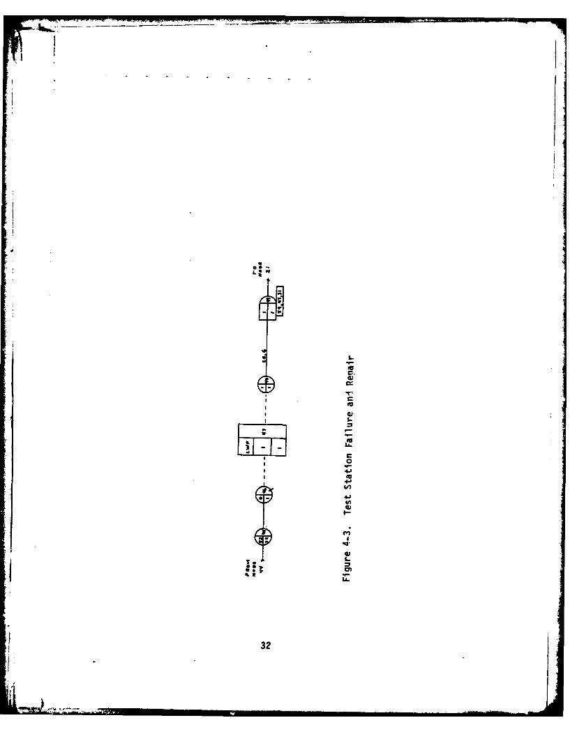
43 traverse a path to free node-44 which frees the test station resource

so that it may be allocated to any waiting transaction in queue nodes

25 through 30. F node-44 also routes the transaction to R node-45.

Test Station Failure

Simulation of test failures is accomplished by R node-45 which acts

as a counter. The number of transactions required to release the node

is set at the mean number of LRU repair actions between test station

failures as estimated by the test station vendor [4, 29]. The place-

ment of the network section of figure 4-3 at the end of the repair cycle

is a matter of networking convenience. In actuality it is more likely

that a test station failure would be discovered at the beginning of a

LRU repair task, but the model can not differentiate between the end of

one task where the test station is released and the beginning of the

next task where the test station is allocated since there is no time

delay involved.

When R node 45 is realized, a transaction is released to Q Node-46

and because of the priority established for this task, transactions

entering this queue will be allocated a test station ahead of any LRU

waiting In queues 25 through 30. The test station failure transaction

is routed from the queue through R node-48 to a repair activity. Upon

completion of repair, the test station Is realeased by free node-49

which allows LRU repair to begin. F node-49 routes the transaction to

be absorbed by R node-21. The box at the bottom of free node-49 is the

31

USO -

9.

3;

L.9-

I ig

a,

C

0

* a,I 1-

.9-

0

e 'I,0. 4-)

Ina)I-

N- I

a,tO

.9-

&A.

32

method by which test station allocation is prioritized. As indicated

by the numbers 59, 47, and 31, test stations will be allocated by node

59 before node-47 etc.

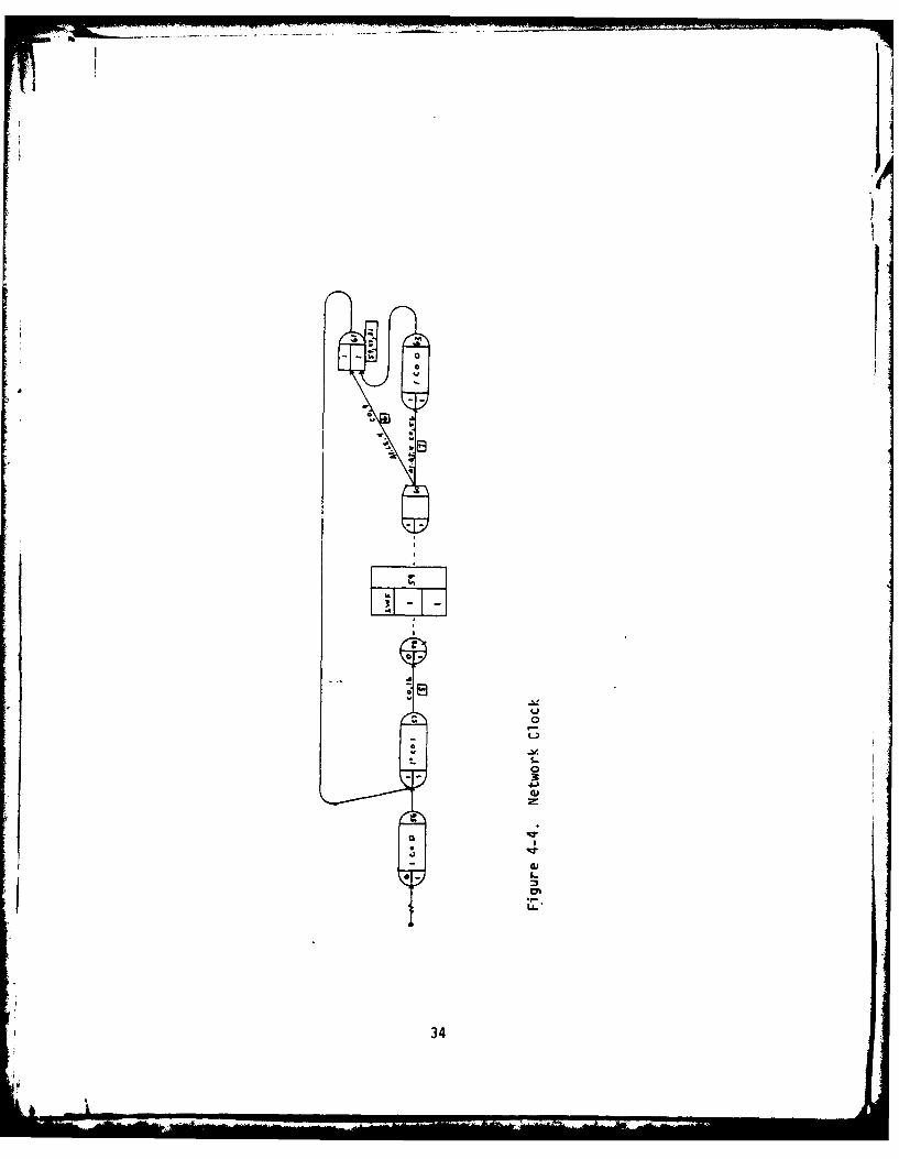
Control of Time

A network device to control the number of hours of flying operations

each day was previously mentioned. The network section of figure 4-4

is the network "clock" which controls periods of flying and periods of

LRU repair. The source node generates a single transaction with the

value of attribute-i set to zero. When R node-57 is realized, the

attribute value is increased by one and activity five begins. While

activity five is in progress, node-5 of figure 4-1 is in the network

and flying occurs. Upon completion of activity five, a nodal modifi-

cation r'eplaces R node-5 with node-62 which routes all transactions

back to Q node-3 and all flying of sorties as indicated by realization

of R node-5 stops. The transaction, upon completion of activity five,

enters Q node-58 and since this allocate node has the highest priority

of all allocate nodes, a test station will be allocated to this trans-

action as soon as it is available. In this manner, shifts are simulated

with the restriction that once a job is started, it will be completed

before the shift ends. R node-60 is a regular node with conditional

take-first branching. The top branch is traversed if attribute-I is

less than or equal to 4. Thus, five days of operating 16 hours and

notoperating 8hours will result in simulation. When attribute-I

33

0 .8

00r0

0-L

343

reaches 5, the transaction will traverse the lower branch emanating

from P node-60 and operations will halt for the weekend. The two

activities emanating from R node-60 are labeled activities emanating

from R node-60 are labeled activities 6 and 7 and upon completion of

these activities, nodal modification replaces R node-62 with R node-5

and sortie generation begins again. Completion of activity 7 also

causes realization of R node 63 which resets the value of attribute

1 to zero so that upon realization of F node-63, a new week begins.

35

I.

jt

44

' ;6

36I

V. MODEL VALIDATION

Verification of Model

Hogg states that "verification of simulation results is a complex

problem" [16]. Comparison of analytic results with simulation data

must allow for the statistical variation inherent in simulation. Differ-

ences will occur due to the approximation of distributions by drawing

random deviates. Since these differences are known to exist, comparison

only yields evidence of model verification and provides no proof of

accuracy.

Within the Q-GERT model of an Air Force Avionic Intermediate Main-

tenance Shop system, transactions occur due to a draw from a distribution

and the path each transaction follows is determined probabilistically.

Finally the time each transaction is in the system is determined by

resource availability and a draw from a distribution. The choice of

simulation as a method to study this sytem was made due to a lack of

analytic ability to model such a process.

Analytic Estimation

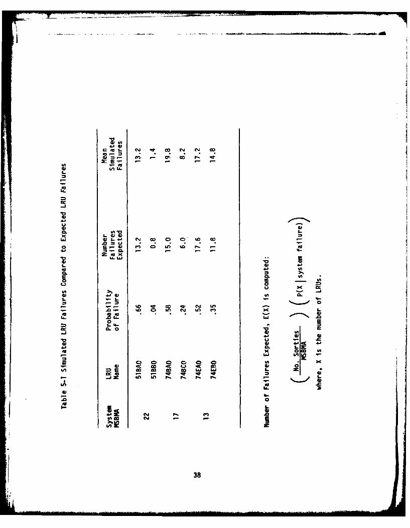
Analytic estimation of the output for the number of LRU failures

and the mean time to repair LRU failures can be calculated. Table 5-1

shows the expected number of failures of each type LRU based upon an

average 20 sorties flown each day and the prescribed system failure rate

and the removal probabilities associated with each LRU. The mean number

37

c a C~j -c co C4 Go

03 4n LL.

0)

4)0.

Lai EnV L.4 c ) Q.o

~Z0 E K r: r

4. = C2t to

03 ~ 4 4) nC

S.La *.-.

0.0E

c.c 0. 0

0 0 cI- wI

E 0) 0 0 Cp Q Q E

E3 co ca co .co 03 .. 2

go '4--qwr 4

4Lb CL

38

of failures over five simulations compare well with the expected number

of LRI' failures.

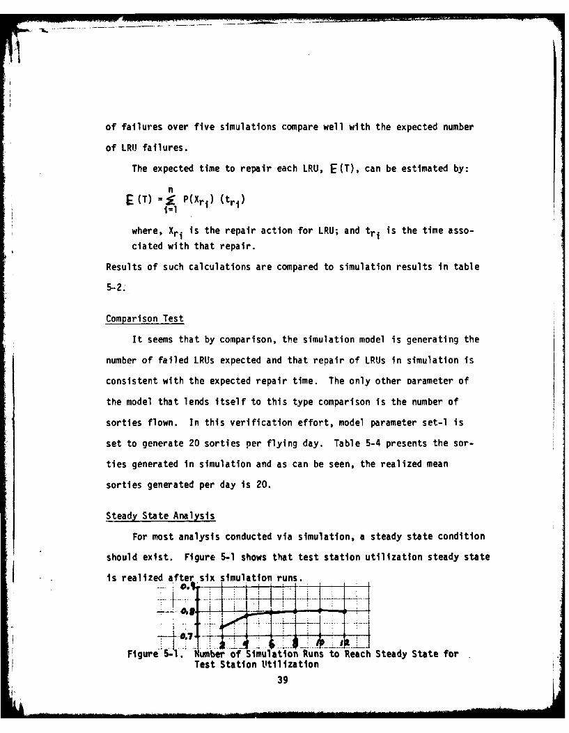
The expected time to repair each LRU, E(T), can be estimated by:

n(T) = P(Xri) (tri)l=l

where, Xri is the repair action for LRU; and tri is the time asso-

ciated with that repair.

Results of such calculations are compared to simulation results in table

5-2.

Comparison Test

It seems that by comparison, the simulation model is generating the

number of failed LRUs expected and that repair of LRUs in simulation is

consistent with the expected repair time. The only other Darameter of

the model that lends itself to this type comparison is the number of

sorties flown. In this verification effort, model parameter set-I is

set to generate 20 sorties per flying day. Table 5-4 presents the sor-

ties generated in simulation and as can be seen, the realized mean

sorties generated per day is 20.

Steady State Analysis

For most analysis conducted via simulation, a steady state condition

should exist. Figure 5-1 shows that test station utilization steady state

is realized after six simulation runs.

. •0.. ; i

Figure'-l. Number of Simulation Runs to Reach Steady State forTest Station Utilization

39

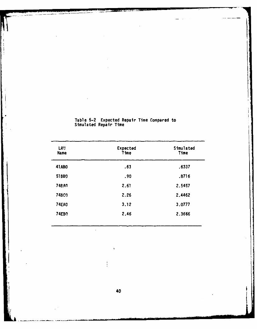
Table 5-2 Expected Repair Time Compared toSimulated Repair Time

LR'J Expected SimulatedName Time Time

41ABO .63 .6337

51BBO .90 .8716

740Anl 2.61 2.5457

748CO 2.26 2.4462

74EAO 3.12 3.0777

74EBO 2.46 2.3666

40

VI. COMMAND LEVEL DECISIONS

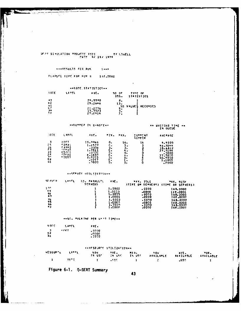
Decision Analysis with Q-GERT

Statistics are computed in simulation that describe parameters

of the system such as: test station utilization; number of LRU

failures; average time in the system; average number and time in the

queue; and number of sorties accomplished in simulation. Q-GERT

Summary Reports provide all of these statistics as output and all

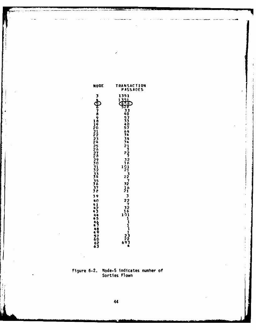
but the number of sorties accomplished are read directly as shown in

the output example figure 6-1. The number of sorties accomplished

equals the number of transaction passages of R node-5 as shown in

figure 6-2.

Following is a discussion of the analysis conducted using the

Q-GERT model of Chapter IV. The analysis herein illustrates the

potential of Q-GERT simulation as a method to aid management in

decision making. The examples used do not exhaust the list of ques-

tions managment can put to Q-GERT analysis but are representative of

that list. Analysis is discussed where management must determine:

1. the number of test stations to purchase relative to the

number of sorties flown each day,

2. the number of test stations to provide the maintenance organ-

ization relative to costs associated with LRI repair,

3. the number of spare LRUs to purchase to support a specified

sortie rate,

42

S.r~ I qUM AT IONJ OR %7 TS0 DY I y .1ELLnATF 9/ 29d 1979

FLAPSWC TIFF FOP fU lVkOO

*f0ES7AT!ST ICS..%oE LA Lf; AVE. 140 Or TY3r OW

05s. STATISTICS4' 29.5590 8

42 25.2646 13. 1!.23%8 VA YLUES RECOQDE3

1). ?923 3. 1p27.E414 1

KU ME P JP; G-PiOrE- * WAITIC6 TIVEr%4 OUCUE

*0 LAPFL AVE. U[: 4* Uv'rPdT AVEPAGENPPER

3 A~rT !5.14966 0. 16. 1& 4.9220_5 I~~.e.537 1). 3 634

26 -- A' Q3 .3336 0. 2. 0 183.68127anI. 79t 1 0. 4. 337.7184;s 'C!" .0130 0. 0. 0 .00C02c "A0 4.C490 0. 6. 5 37.7620? , r 1E912.0213 0. 6. 4 q0.QOlO51 .Oj57 0. 1 . c 1 .1 9q5'46 .100C 0. 0. 0 .1000

S''4 LA-CL -1.0. 9ARALL!. AVE. VAX. IDLE MAX. RUSYSERVER$ (TINPE 00 SEOVERC3 CTI-E OR SEP VERSI

1 1.0000 .CCOO 169.0000@9 C I.Ocl~ .00110 161.000092 1.00013 . a0o.,0 166.30000 7 1 1.0000 .0000 l~e.OOOCIt 1.03010 . Clo 166.300095 1 1.ConO .OOCO 166.0300%a1 1.az 001.COCO 168.003C03 1 1.0000l .0000 161.0000

0-10. BALK?'04 PER UA'? T19E..

'~oro LASVLar

46

.. 4rSOJR'F lJTILIZTOskESOUP'L LA~v1 *0w AVE. 14). "cV AVE.

tSO us US?- INi t us- AVAILAPLE AVAILAI!LE AVAILAtLE

Figure 6-1. Q-GERT Summary 43

NODE TRANSACTIONPASSAG-ES

3 1351

7 33 >8 40 :

9 5718 3319 4020 5?21 61422 3423 31424 3425 2126 327 22

2S 729 3230 if31 1 G132 21

322

35 736 3237 163E' 2139 340 2241 742 3243 1644 101485 146 147 148 149 157 2360 2262 69363

igr6-2. Ne-5 indicates number of

Sorties Flownr44

!44

4. the time period required to complete repair of an existing

backlog of failed LRIJs,

5. test station availability for training when a proposed flying

schedule is given,

6. if the number of failures realized for a given LR' during

some period is representative of the aircraft system estimated

mean failure rate,

7. the dimensions of the storage space required for failed LRUs

awaiting maintenance relative to the number of sorties flown

per day.

Questions of the type illustrated by the first three examples

represent command level decisions, and are discussed in this chapter.

The remaining questions are more of the day to day decision requirements

of local management and will be the topic of Chapter VII. Discussion

of the analysis involved in these decisions is intended to substantiate

the proposal that Q-GERT is a viable tool to he used by Air Force

management during both the acquisition and operational cycle of a weapon

systems life.

Test Station Acquisition Relative to Sortie Requirements

Problems Encountered in Test Station Acquisition

Determination of the number of test stations to purchase must be

made early in the acquisition program. Generally, the only information

available at the time a decision is made consists of estimates of:

45

system mean time to failure; probability of component black-box fail-

ures given the system failure; probability of the type repair action

required; and the mean time to repair for each type repair action.

One other test station utilization parameter that is known is the

number of sorties per day that will be required for each flying unit.

With this information at hand, Air Force managers must determine how

many test stations will be required at each installation responsible

for repair of the specified aircraft systems and the LRUs associated

with those systems. The number of test stations purchased can be

based on the flying units' deployment responsibility. Oecisions made

in this manner will authorize the unit that must support two combat

operating locations two test stations while the unit that remains

intact during combat deployment will be authorized only one test

station.

Authorization based upon this deployment factor has merit in

that it is obvious that to support two separate and independent oper-

ations, a minimum of two test stations is definitely required. The

problem that exists in this method of authorization is that there is

no attempt to determine the sufficiency or support effectiveness of

the single test station.

Development of Decision Criteria

Intelligent decision making concerning the acquisition of test

stations must include the determination of test station utilization

46

based upon mission requirement. In that the number of sorties flown

per day is the measure of a flying unit's mission requirement, the

decision maker must in some way relate this sortie requirement to

test station utilization.

Simulation of the Q-GERT model design of Chapter IV will provide

this much needed estimate of the relationship between the number of

sorties flown and test station utilization. Output statistics of

several simulation runs over a range of sortie rates can be analyzed

using linear regression to estimate test station utilization, depend-

ent on the average number of sorties flown daily. Such a method

requires that at least five simulation runs at each sortie rate be

conducted and that the sorties rates used in simulation exceed the

maximum potential sorties requirement. Requirement of five simulation

runs of each sortie rate is based upon the common practice of using

4 or 5 samples in a subgroup to estimate mean statistics r14]. Simu-

lating at a higher sortie rate than the estimated extreme will insure

that the regression line includes the possible sortie rates of interest.

The regression line determined using output statistics of these simu-

lations may be used to compute the test station utilization factor for

any sortie rate in the range of regression. Confidence intervals about

the mean points of regression are established to provide the manager

with a clearer understanding of the statistic he will use in a decision.

Regression provides data for graphical representation of test

station utilization versus the number of sorties flown per day. This

47

graphical representation is easily read and understood by management.

Management can, with the confidence level described on the graph,

determine the expected test station utilization factor for any desired

sortie rate [6]. This method of decision making will allow management

more knowledge of the system and more confidence in the conclusions

made.

Simulation'and Regression Analysis

As an example of the above described procedure, simulation was

conducted to generate output statistics of test station utilization

for eight sortie rates. The sortie rates ranged from 20 sorties per

day to 90 sorties per day in intervals of 10 sorties per day. Simula-

tion at each sortie rate was replicated five times with the average

test station utilization statistic for each simulation used to compute

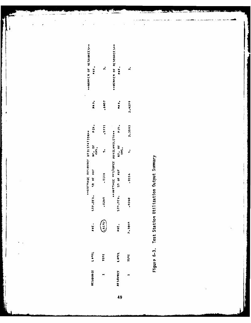
an overall average test station utilization statistic, Y. An illus-

tration of the simulation output used to determine Y is presented as

figure 6-3. Output statistics of Y for each set of simulation runs

were used in conjunction with the appropriate corresponding sortie

rate, X. Table 6-1, presents the simulation output and computations

performed to arrive at the expression:

Yc = .0045 + .0116X

where, X is the number of sorties per day

and Yc is the resultant mean test station utilization;

which gives management the ability to calculate an expected test station

utilization factor for any sortie rate desired.

48

6A

0 0

2. w

04 01

fu

a: 1

2 42

1K 4 K

az Nn1

~ 01

4 49

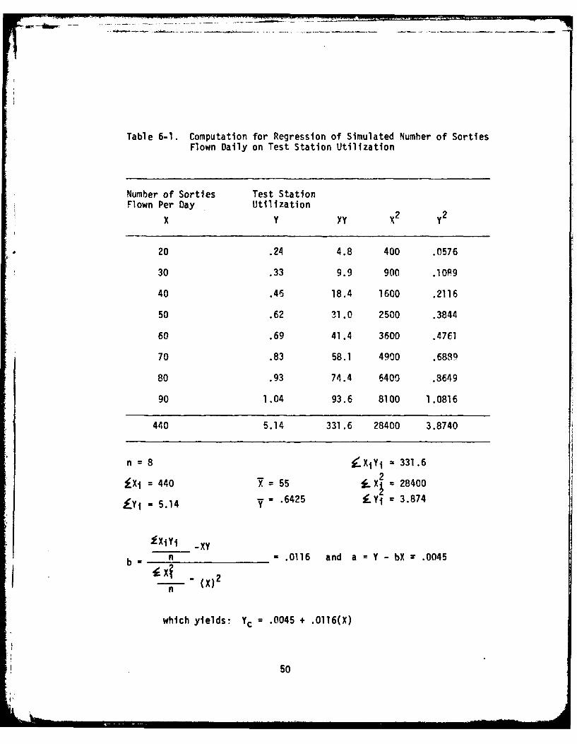
Table 6-1. Computation for Regression of Simulated Number of SortiesFlown Daily on Test Station Utilization

Number of Sorties Test StationFlown Per Day Utilization

x YY

20 .24 4.8 400 .0576

30 .33 9.9 900 .10P9

40 .46 18.4 1600 .2116

50 .62 311.0 2500 .3844

60 .69 41.4 3600 .476.1

70 .83 58.1 4900 .6889

80 .93 74.4 6400 .8649

90 1.04 93.6 8100 1.0816

440 5.14 331.6 28400 3.8740

n 8 XYi-331.6

J-Xi = 440 7 =55 X?.Y- 28400

£Yi = 5.14 v= .6425 Yiv3.874

;Exiy -xy

b ___z__n___ - .0116 and a =Y HX .0045I:xf - Mx) 2

n

which yields: YC .0045 + .0116(X)

50

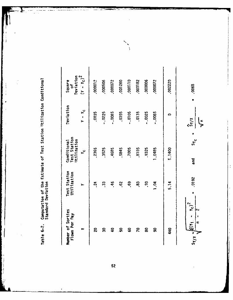
Calculation of Yc for sortie rates over the range of the regression

line enables computation of the conditional standard deviation of the

estimate of test station utilization. Comparison of simulation resultant

Y with computation for Yc to determine an estimated standard deviation

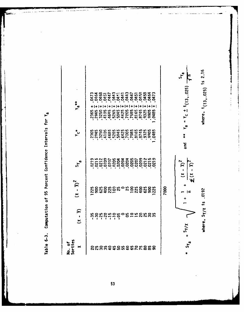
Syc is shown in table 6-2. This standard deviate is used to construct

95 percent confidence intervals about the estimated mean test station

utilization, Ya as shown in table 6-3.

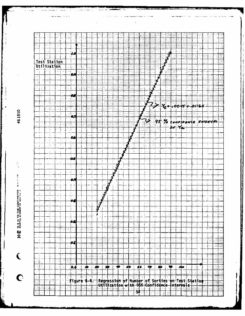
Values of Yc and Ya are used to construct the graph of figure 6-4

which provides management with a means to select the mean test station

utilization expected for a given sortie rate. They will be able to use

this graph with 95 percent confidence that the actual test station util-

ization will be in the interval indicated by the dotted lines.

Decision Rule

Test station acquisition decisions can be made with the aid of

the information provided in figure 6-4. Management has only to deter-

mine the sortie rate which must be supported and then by selecting the

point along the X-axis that represents the desired sortie rate, a point

on the regression line can be identified. From the point on the regres-

sion line that corresponds to the sortie rate of interest, they can

trace across to the Y-axis and read the expected test station utili-

zation.

51

F- 0-0 ) .- U C1.1 .W % 0l 0 CJ W. CA

C~C S.. W) 00 C> 0 . u I.o "'-. I n , 0) CD ) C- ,- 0 0) C4W

0'- > 0) 0 CD Z) 0 CD 0 C) Cl Q.V) 0) >- C0 0 Q C C) 0 0D 0D C0 CO

10 M-

C0

041to +) >- U,) u,) Lc) U, U) LO U, U

N; 0 (C) m. , C C'.) 0> C) C) 0D (D CD 0 CD

rC U

0 4044)S-OC toU)U l U) L ) U

4Jl (f 4 L o ~ 0 -r C) t 0 CM) 0O %D04) n c

(C'4J m, U, r L L) U, ., 00 U, UD

0 0 )4-) I- U) Mt

4-) m0 l m m4)

0

0

4) tIM

f) 11- cJ

4).s- c

%I ) C)

F Uf) 4 W o l 0 0

0- %-.

C3O-

- -- -- ~ -~-- -. C

OrJ -c, -4! T .,m

* I-.

1

14-

I- L V UU, ) LO LOLn U') ) UULU'U') Lit

> G. %0" Or~-o~~, *c DL .Mm : 0 " @ Q3 fc oC hC

C

4- 0- c. J( m. .. .C. .~tn L=.0lCDOOC OODOD O QC)CD0 D

" 0% " ++00

4m r-4- + at

CL 31<

39

in'4-@ wU

4J 0 nC . n n0 nQU)-L

53

-~- - ---- -- ~~

3tii7a ._ ._ . ...

a a ... ... 7-

V I LI * S -I-

7 44

77 -7 w :j = :::7

.. w TL.J*- ~ --- ---.--.- -- -~ --.--- I..-.-a

-i Im

wV j

A~ :1 f .

--I-- -711a ?---,---- --- -oil=

C~~~ AC~rs ::4twbro1 a .S..

.. t.. ..H .t...

Test Station Acquisition Relative to LRU Repair Costs

Assumption of Repair Criticality

Assume that the number of sorties required per day is not the pri-

mary measure by which test station support requirements are established.

During the period of initial weapon system build-up it is possible that

spares levels will not be at the estimated requirement. Due to the

complexity of manufacturing, the contractor may not be able to provide

production and spare level demands for some critical LRUs. Such a situ-

ation may make the repair cycle time of a LRU more important since this

repair time represents a time constraint on the generation of sorties.

If spares for a particular LRU are not available, and that LRU is a

critical flight item, the aircraft must wait until the LRU is repaired

before it can fly.

Under such circumstances, management would like to know more about

the time to repair the LRV in question. The repair time with one test

station available could be compared to the repair time when two test

stations are in use to measure the effect of having an additional test

station available.

Repair Time Probability Distribution

Analysis that will provide probability distributions of repair

cycle times for LRUs can be accomplished using Q-GERT. Statistic node

histograms can be requested for the statistic nodes associated with

the LRUs of interest. Each histogram will provide a graphical repre-

sentation of the mean repair cycle time for the simulation runs with

55

a table listing the relative frequency and the cumulative frequency

of those mean repair cycle times. The cumulative frequency describes

the probability distribution of repair cycle time that may he used in

the decision process.

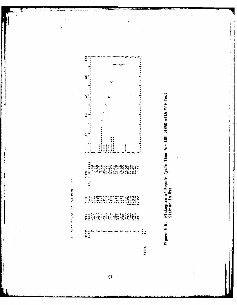
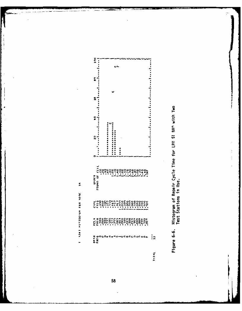
Simulation of Alternatives

Twelve simulation runs were conducted with both one and two test

stations in use. Analysis of the output from these simulations is con-

ducted for LRU 51BAO as an illustrative example of the method. Histo-

gram output from simulation is shown as figures 6-5 and 6-6. The first

figure displays simulation results of one test station and the second

figure displays the simulation of two test stations in use. The sta-

tistics listed under column heading CUML FREQ in these figures can be

interpreted as the probability that the repair cycle time is equal to

or less than the corresponding time in the column heading UPPER BOUNTI

OF CELL. As can be seen in fiqure 6-5, with one test station, the

probability of the repair cycle being six hours or less is .083, while

the maximum repair cycle time of figure 6-6 is 1.8 hours. If management

can determine the time period that is acceptable for repair, they can

use these statistics to make the decision between one or two test sta-

tions.

Determination of Decision Rule

Let's assume that the situation described in the preceding para-

graphs will exist for about one year. That is, in one year, spare LRUs

56

Lr . .T r Ccf-g c r

. . .. . . . . .

4 4.)

- e.-.

. . . . . ...

* . I-

.LC.

571

* .* I...

-I

;- 0.

o I 0• en

-'r-~o~e-~-c

D,-

57?:Eu

UP

- ---- -

4J 4.)

c C or- ,n0CC0 ca0cC 0

* ..

58S

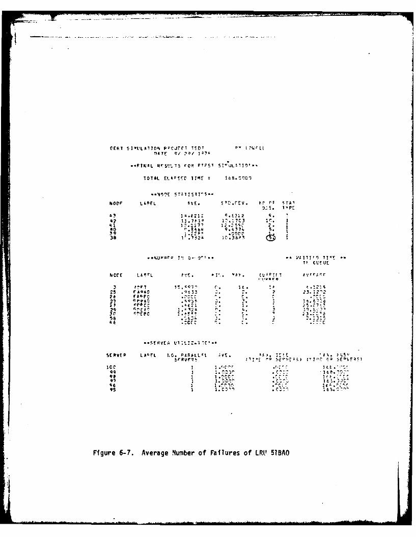
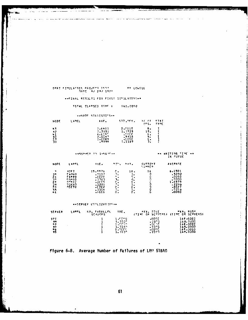
will become available. The cost of an aiditional test station for one

year is estimated by management at $l00,000.0 and repair cycle time

is valued at $50.00 per hour. With these cost estimates, the histogram

output of figures 6-5 and 6-6, plus the expected number of LRU failures

per week at the sortie rate simulated as indicated in figures 6-7 and

6-8, a decision rule may be determined.

The expected number of failures is 5 per week which is 260 per

year. The expected cost of these failures is computed as:

E(c) = 260tP(t)C

where, t repair timeP(t) probability of the repair time

and C cost of repair.

Tables 6-4 and 6-5 present the results of these calculations which show

that it is less expensive to expend the $100,000.00 for an additional

test station for a year than to onerate with just one test station.

Spare LRU Acquisition

LRU Constraints on Sorties

Test station acquisition is only one of several decisions involved

in the total avionic maintenance support area. In the first section of

this chapter, test station utilization was considered independent of

the number of spare LRUs available. This assumption is valid in that

test station utilization is independent of whether the LRU is constrain-

ing the aircraft. The fact is that such a constraint will effect sortie

generation and must be a consideration by management. If a given LRU

59

CEPT S'1D.TA1I0% PPCJrft7 TSV P IM KLt

TOTAL ELS8C TIME 168. :1012

NiOPF Lt!'rL !VE S :.rEV. P. r r CTAI:- . i -,PE

42 13 . 7 1' V. :73 C ~ 3II2 1 ~ 2 S 2. 140~:6 9.I..'74.S. I39 2.2p, 0C38 1 .72 !C3PI

.*%Uw~~kTp Vt !' TlE

NCCE LAeL f ! 1. . VIY. (L~ctf 7 yrt

3 P!. I. leF5 AQ : O 2 23.i2~

26 rcc~* -**

r8 c ~ 57 .7 r -

3c V E p'C'' .. ! r

56 1.1) t :4

9e i .t:.

Figure 6-7. Average Number of Failures of LR(I 51BAO

C*iTc "UATTk P; UrCJ'l V~'y LCEL

IaTE q/ 201 Iq7*

*.clNAL RE7S.jLT3 FOR FIRS'LTVs

TOTAL S1..hDSED T~ 16e11010

rUc0' LA=FL £Vjr. S~.-% N( c; CTATr:2S. TyOE

43 ? .6 4 i1 2 .* 115 8. I'42 !.3351 1.7'725 15. 1

"C7 ?. OC4 .14iS '4. 1? i. 2 2e5 . cC00 I1. It

33 .099az .1 169 5

-*6PJm4E? 'I P13W'~ ~AITIG 'ImE .

NOflE LAPrL tVE. E u beP CE K, AVEPAr.E'U "Q1E 0

Schr? 115.C? c7t c. 16. 16 6.150125 ~APAO .1'157 . 1. C.5292

2F r. ,- Cc F 6 c. 1. 1 .4979'Q 'IWAD .Z201 :% 1. 0 .22:16i3 (go ~ .C1e2 C. I1. EO2

-5q.1C c 6 1. 0 .f,2 16'46 .C-CC C .0. .0000

*..rPIEF LIVILIZAT 1rI.-

SEPVER LS*'L "'Cl. FOPALLFL 1VE. pix. !TIE VAX F'SVS~r-?PpS (T!J- OP b~~PSJ ITI~ OR SEDVERS)

I r c I r" .0^,r It8F0c~c^09 1 t.CCC' .cO^ 6.iO

'45 I.CCC 68 .00cO97 1 1. C0o' .CC0 188.2000

16; 1.CC .'Onc 160: on95 1 .C'.CC16 000

Figure 6-8. Average Number of Failures of LRI' 51BAO

61

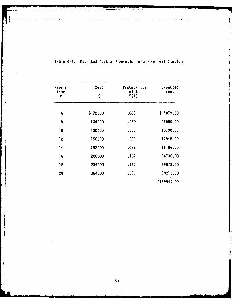
Table 6-4. Expected rost of Operation with One Test Station

Repair Cost Probability Expectedtime of t cost

t C P(t)

6 $ 78000 .083 $ 1079.00

8 104000 .250 26000.00

10 130000 .083 10790.00

12 156000 .083 12948.00

14 182000 .083 15106.00

16 208000 .167 34736.00

18 234000 .167 39078.00

28 364000 .083 30212.00

$1 69949.00

62

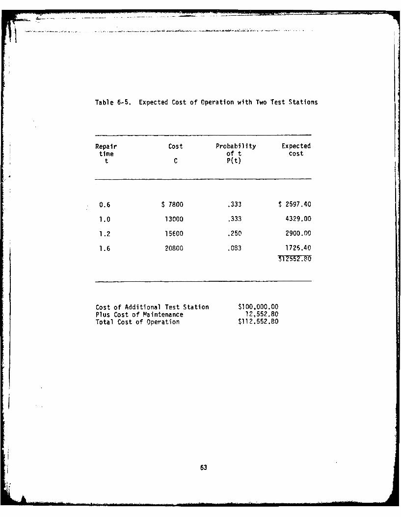
Table 6-5. Expected Cost of Operation with Two Test Stations

Repair Cost Probability Expectedtime of t costt C P(t)

0.6 $ 7800 .333 $ 2597.40

1.0 13000 .333 4329.00

1.2 15600 .250 2900.00

1.6 20800 .083 1725.40$1 2552.80

Cost of Additional Test Station $100,000.00Plus Cost of Maintenance 12,552.80Total Cost of Operation $112.552.80

63. _

is aircraft constraining, Air Force managers would like to establish

spares levels such that no flight is ever lost due to the lack of a

spare LRU. Although this is generally not economically feasible,

there is a definite need to know what level of spare LRUs would pro-

vide such support.

The spare LRU requirement issue, like the test station decision,

must be resolved long before empirical data is available. This situ-

ation lends itself to simulation with the use of estimates of failure

and repair parameters just like the test station utilization question.

The model of chapter IV must be modified to provide output statistics

describing the demand distribution for a given LRU. Once again the

LRU 51BAO will be used to illustrate network modification and the

eventual decision analysis.

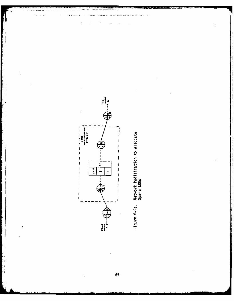
Required Model Modification

The modification required involves the addition of four nodes

and a resource for each LRU to be analyzed. Since this example involves

only LRU 51BAO, the modification of the network branch between R node-18

and Q node-25, and the branch between statistic node-38 and F node-44

is required. As shown in figure 6-9a, the insertion of Q node-70 and

allocate node-71 make the availability of a spare LPU necessary before

the failed LRU may be processed for repair. Pegular node-72 is neces-

sary since in Q-GERT, a 0 node can not follow an allocate node. Free

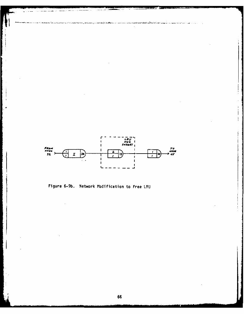
node-73 is inserted between statistic node-38 and free node-44 as shown

in figure 6-9b, to free the LRU after repair is completed.

64

44

S.l

wC.)

t I-

lo 0L

650

N~me"

Figure 6-9b. Network Modification to Free LRIJ

66

Simulation to Determine Demand Probability Distribution

With these modifications and the establishment of the LRU

resource level high enough to meet any demand, simulation is used

to determine the demand distribution. Knowledge of the distribution

for the probability of demand will aid management in the decision

concerning the number of spare LRUs to purchase.

As in previous simulation analysis, management must have enough

knowledge of the system to determine the number of sorties required

and the work shift structure to be used. Herein it is assumed that

40 sorties per day is the flight requirement and the work week con-

sists of two 8-hr. shifts, operating five days per week. The LRU

spare resource level is set at five, which seems reasonable based on

previous simulation results.

Sixty 1-day simulation runs were conducted and the demand for

LRU 51BAO was used to construct table 6-6. These simulation observa-

tions were grouped according to the number of demands and probability

distribution p(D) and cumulative probability P(fi) estimates were com-

puted as shown in table 6-7.

Application of Inventory Decision Model

Since spare LR stock has the same properties of inventory, a

discrete inventory decision model is used to help structure a decision

rule for spare LRIJ purchases. First it is assumed that a cost can be

determined that would represent the loss of a sortie due to demand

67

A!

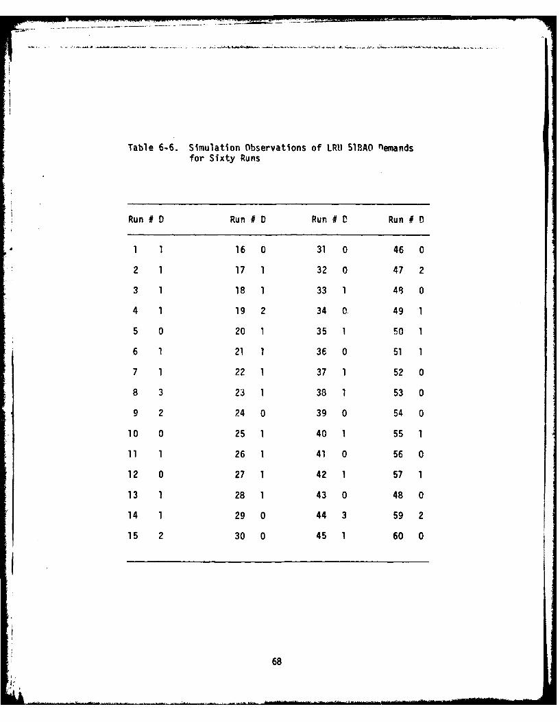
Table 6-6. Simulation Observations of LRU 51BAO nemandsfor Sixty Runs

Run # D Run # D Run #D Run #

1 1 16 0 31 0 46 0

2 1 17 1 32 0 47 2

3 1 18 1 33 1 49 0

4 1 19 2 34 0 49 1

5 0 20 1 35 1 50 1

6 1 21 1 36 0 51 1

7 1 22 1 37 1 52 0

8 3 23 1 38 1 53 0

9 2 24 0 39 0 54 0

10 0 25 1 40 1 55 1

11 1 26 1 41 0 56 0

12 0 27 1 42 1 57 1

13 1 28 1 43 0 48 0

14 1 29 0 44 3 59 2

15 2 30 0 45 1 60 0

68

it.

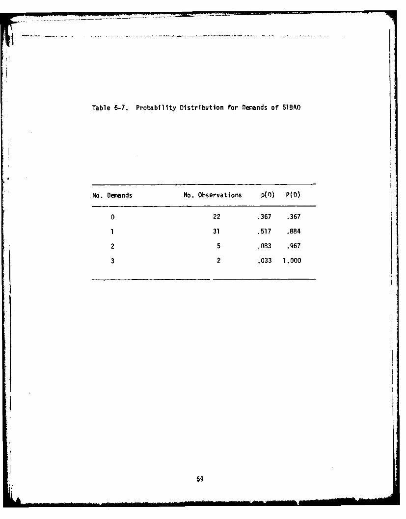
Table 6-7. Probability Distribution for Demiands of 51BAO

No. Demands No. Observations p(rn) p(n)

0 22 .367 .367

1 31 .517 .884

2 5 .0l83 .967

3 2 .033 1.000

69

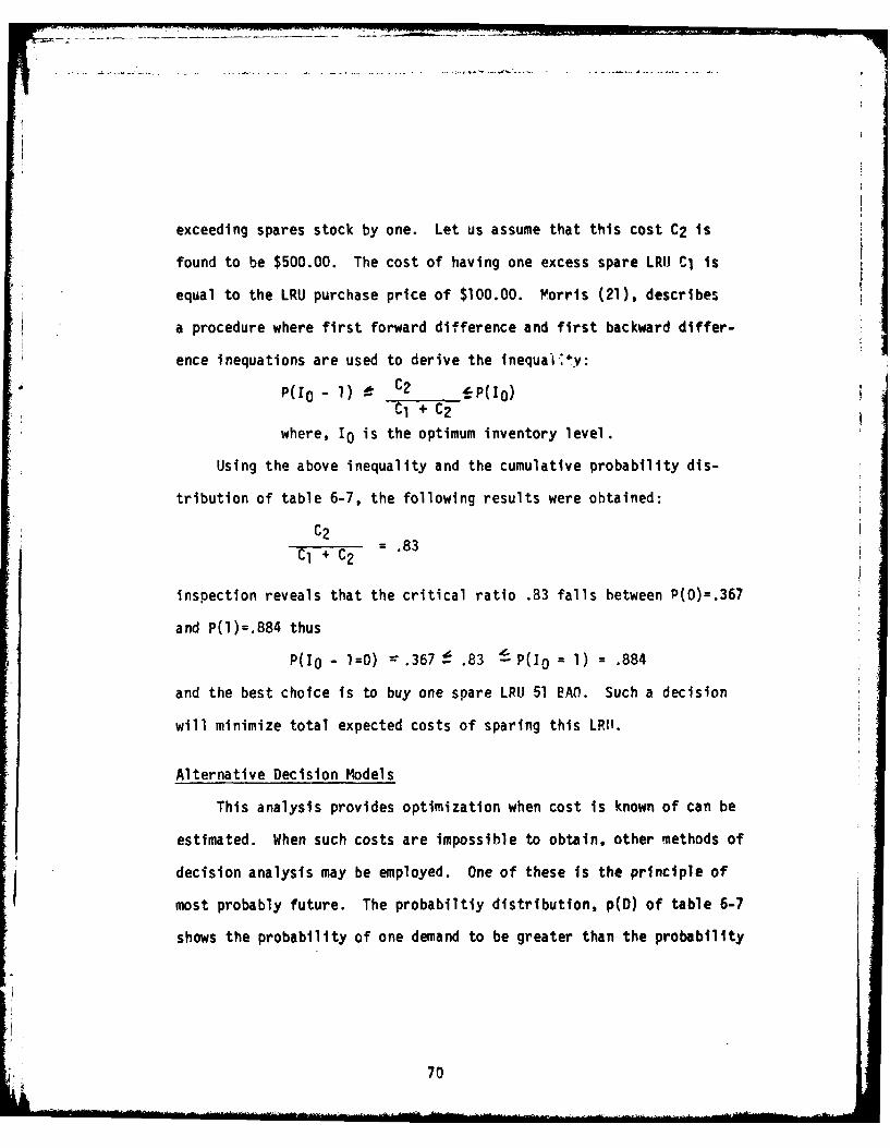
exceeding spares stock by one. Let us assume that this cost C2 is

found to be $500.00. The cost of having one excess spare LRU C1 is

equal to the LRU purchase price of $100.00. Morrls (21), describes

a procedure where first forward difference and first backward differ-

ence inequations are used to derive the inequai. 4 y:

P(oo - I) C2 PCl + C2

where, 10 is the optimum inventory level.

Using the above inequality and the cumulative probability dis-

tribution of table 6-7, the following results were obtained:

C2 -= .83Cl + C2

inspection reveals that the critical ratio .83 falls between P(0)=.367

and P(I)=.884 thus

P(IO - 1=0) -.367 t .83 ! P(Io = 1) = .884

and the best choice is to buy one spare LRU 51 PAD. Such a decision

will minimize total expected costs of sparing this LRII.

Alternative Decision Models

This analysis provides optimization when cost is known of can be

estimated. When such costs are impossible to obtain, other methods of

decision analysis may be employed. One of these is the principle of

most probably future. The probabiltiy distribution, p(D) of table 6-7

shows the probability of one demand to be greater than the probability

70I

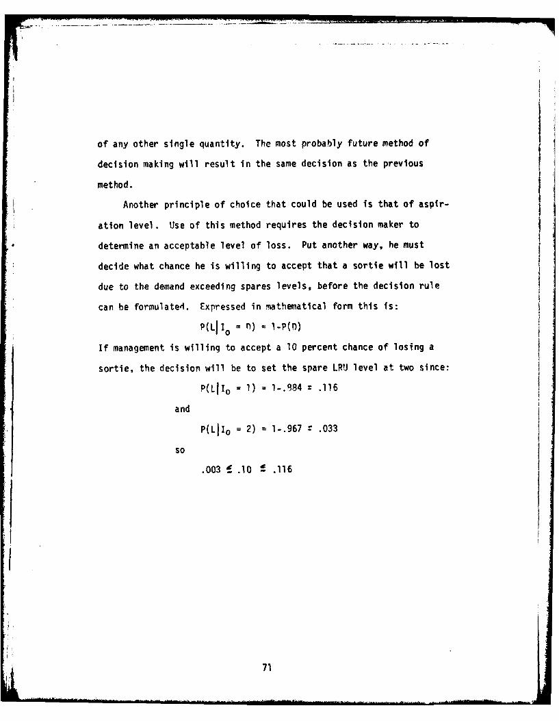
of any other single quantity. The most probably future method of

decision making will result in the same decision as the previous

method.

Another principle of choice that could be used is that of aspir-

ation level. Use of this method requires the decision maker to

determine an acceptable level of loss. Put another way, he must

decide what chance he is willing to accept that a sortie will be lost

due to the demand exceeding spares levels, before the decision rule

can be formulated. Expressed in mathematical form this is:

P(LJI0 = r) = l-P(D)

If management is willing to accept a 10 percent chance of losing a

sortie, the decision will be to set the spare LRU level at two since:

P(L1Io = 1) = 1-.984 z .116

and

P(Ljlo = 2) = 1-.967 r .033

so

.003 i .10 - .116

71

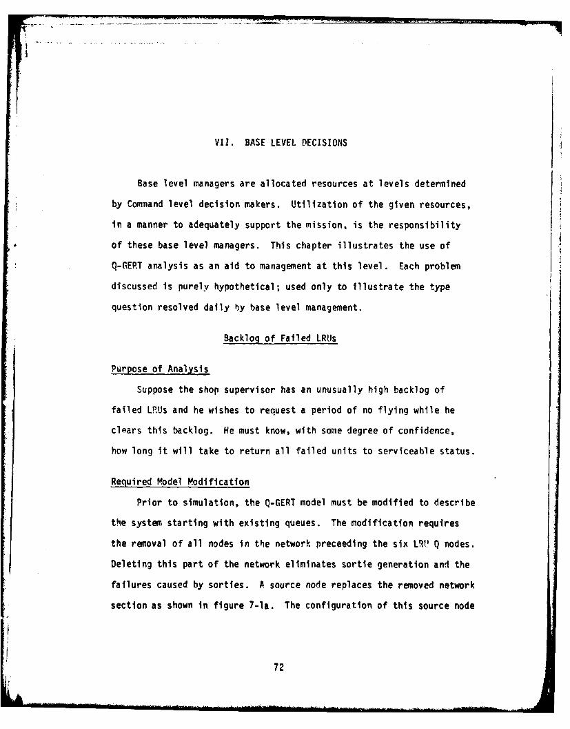
VII. BASE LEVEL DECISIONS

Base level managers are allocated resources at levels determined

by Command level decision makers. Utilization of the given resources,

in a manner to adequately support the mission, is the responsibility

of these base level managers. This chapter illustrates the use of

Q-GERT analysis as an aid to management at this level. Each problem

discussed is purely hypothetical; used only to illustrate the type

question resolved daily by base level management.

Backlog of Failed LRUs

Purpose of Analysis

Suppose the shop supervisor has an unusually high backlog of

failed LRUs and he wishes to request a period of no flying while he

clears this backlog. He must know, with some degree of confidence,

how long it will take to return all failed units to serviceable status.

Required Model Modification

Prior to simulation, the Q-GERT model must be modified to describe

the system starting with existing queues. The modification requires

the removal of all nodes in the network preceeding the six LR.' Q nodes.

Deleting this part of the network eliminates sortie generation and the

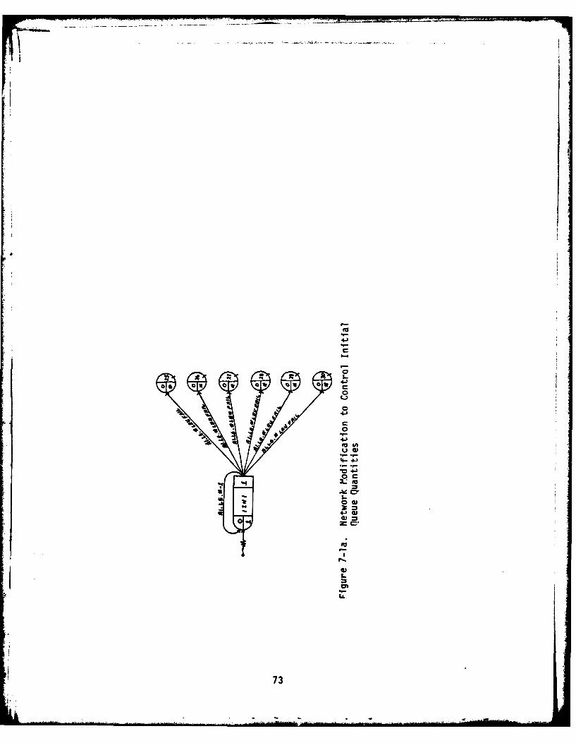
failures caused by sorties. A source node replaces the removed network

section as shown in figure 7-1a. The configuration of this source node

72

4-)

-00-

4 -40

- S-

it 0

4* 0)

LL.

734

is such that it generates the desired number of failed LRIIs. The

source node has conditional take-all branching with a branch leading

to each of the LRU queues. Another branch emanating from the source

cycles back to cause successive realizations of the node. The source

node also serves as an increment node and incrementally increases the

value of attribute-l by one on each realization of the node. Each

branch leading to a Q node has the condition Al.LE.#, where # is the

number of failed LRUs desired in the queue at the beginning of each

simulation run. The branch returning to the source node will have

the condition Al.LE.#-I, where # is the greatest number of LPI's desired

in any of the queues. This will stop the source node from creating

transactions once all the queues reach the desired number of failed

LRUs.

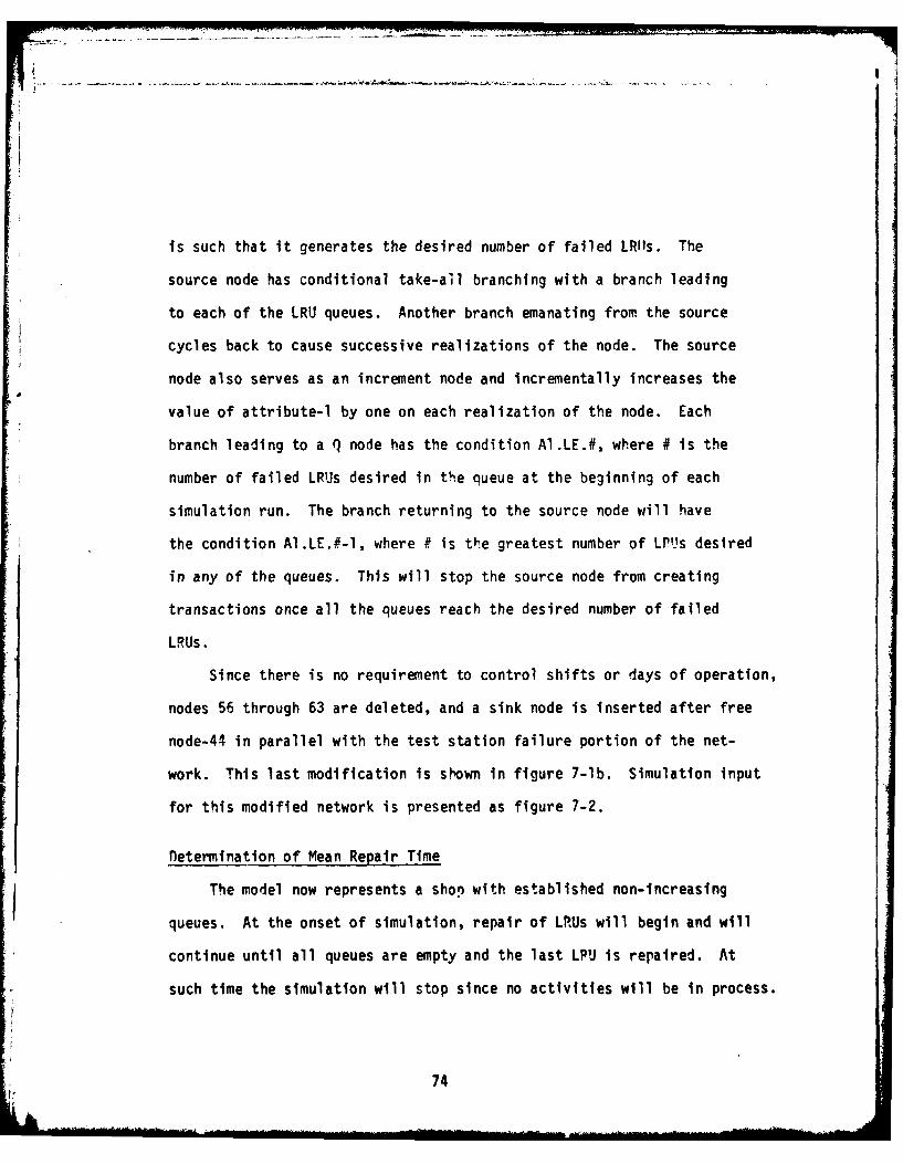
Since there is no requirement to control shifts or days of operation,

nodes 56 through 63 are deleted, and a sink node is inserted after free

node-44 in parallel with the test station failure portion of the net-

work. This last modification is shown in figure 7-lb. Simulation input

for this modified network is presented as figure 7-2.

netermination of Mean Repair Time

The model now represents a shop with established non-increasing

queues. At the onset of simulation, repair of LRUs will begin and will

continue until all queues are empty and the last LPU is repaired. At

such time the simulation will stop since no activities will be in process.

74S1 b .. .

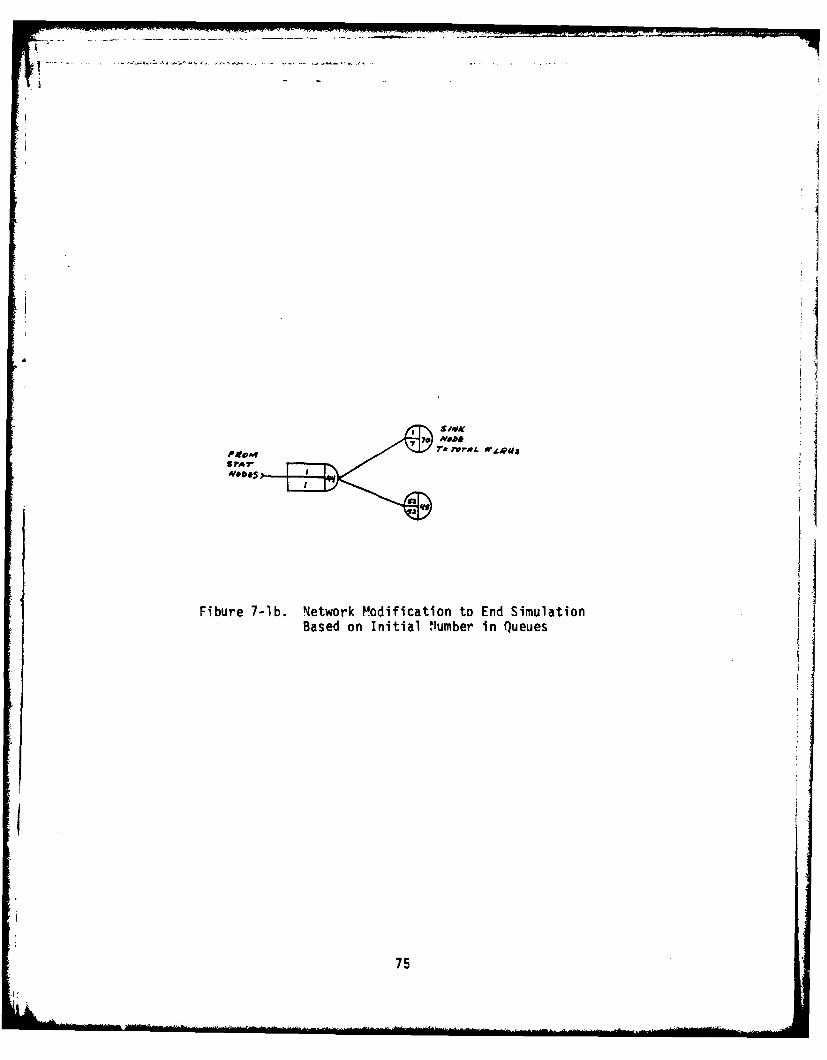
ro JVFAL WAEM.

Flbure 7-lb. Network Modification to End Simulation

Based on Initial 'Number in Queues

75

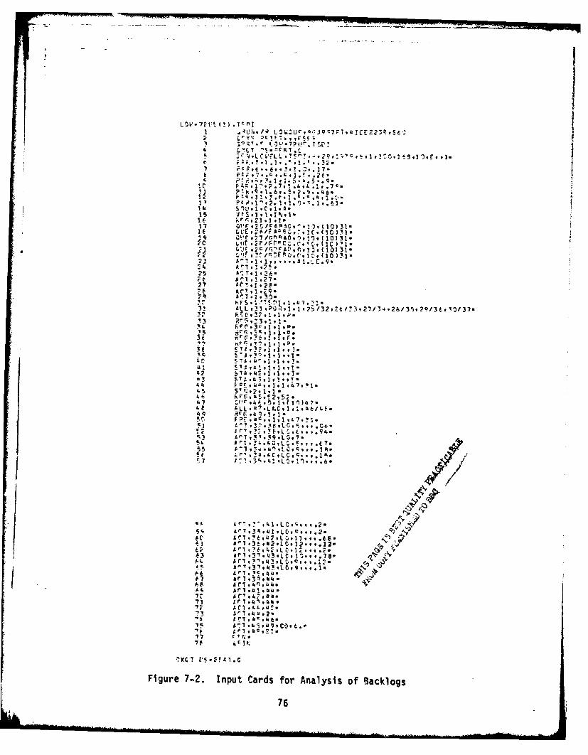
-L C ',F L

7 7-

11A

S11 N

i9 W'T1,77/nA9 ' 0 123 ,!i 2 FLLr,3 r-C *G,.1,2/3,9 t!327#4.)/3?2/3I'o37

A 171 '1

32 F , 1,I" 1 * P 1

3. "t 1.1 Y

?7 1%"r- 7LI 1 VD.~ I~~

4-A42 455 ) 1*9

27 r 3 . aj 1

77

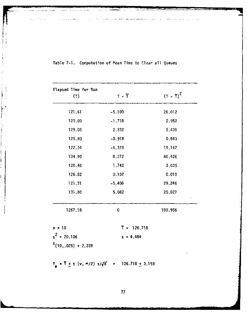
Table 7-1. Computation of M~ean Time to Clear all Queues

Elapsed Time for Run2(T) T- (T-)

121 .61 -5.103 26.012

125.00 -1.718 2.952

129.05 2.332 5.438

125.80 -0.918 0.843

122.34 -4.378 19.167

134.99 8.272 68.426

128.46 1.742 3.05

126.82 0.102 0.010

121.31 -5.408 29.246

131.80 5.082 25.827

1267.18 0 180.956

n =10 T= 126.718

= 20.106 s = 4.484

t (0,.25)= 2.228

a + t (-e, -%12) s/.,ii 126.718 + 3.159

77

Simulation output summary statistic ELAPSFD TIME FOR RUN illustrated

by figure 7-3 can be used to compute a mean time to clear all queues.

Statistical inference tests with the Stud.,nt-t distribution is then

used to establish confidence intervals about the mean time to clear

all queues.

An Example Simulation and Results

For the purpose of analysis, simulation was conducted with ten

failures in each quque upon activitation of the model. Ten simulation

runs were completed and the time statistic from each was used as shown

in table 7-1 to compute a mean time to clear all queues. Ninety per-

cent confidence intervals about the mean were computed with the results

showing the expected time to clear the queues being between 5.1 and

5.4 days. With this information, the superivsorcould,with 95 percent

confidence, support a request for a six day stand-down.

Planning Training

Purpose of Analysis

Suppose the shop supervisor knows that 20 sorties per day are

scheduled for the next week and he must conduct some training that will

utilize the test station making it unavailable for aircraft support.

The present hours of operation for the shop are two 8-hour shifts 5

days per week and the supervisor wishes to maintain these hours of

operation. He wants to know how many hours can he devoted to training

78

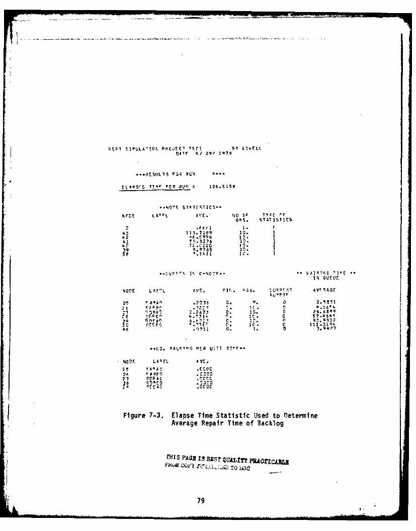
C(EF7 SIPULJ.'10t. PF.CIECF 'Sri E'r LOkELLGAr -./ 291 1979

ELAPS:'r Tlyr rCR R12' 126.1150

%CrE LAcrL AVE. N~O OF TYPE !%FOpS. STAlISTICS

21. F43113.7189 10. 7

£52 At%.=995 1ll. I41 - t. 276 10I. 1

4C 3.C 220 10. 139 Z. 765 1C. 1

114 OUEt'E

W LIF Fr

25 r DA .2035 . 2. '!!l

2- , CA 2.2623 0. 105. 0 25. be"17.~rL C' Mc 0 C.&9

29 r, Sn fr .07 C . n0 R ~ 3. 9 813 1 0.tE o ~ . '?I F IC. 0 111I.31 Q4

1693; C. 1. a 3.94P~7

N .E LAQEL A VE .

2 C ~ A IF 1 .1c27 CCrAC TC28 0OC 02C t C. .C(C

Figure 7-3. Elapse Time Statistic Used to netermineAverage Repair Time of Backlog

'H'S PAaB IS BEST QUAZITY pjjA~CrZA=~

79

, 4

co. .4.

hr . ..~ N . .. .

v L L. L

-'.0'

2 .*

r c.C

. . .. .f . ...

cr.r L: LL CuL L 16 4 Lw:1 ;N

!kl Z. Z = 5'Un - 0

C.. C *.80.0w.S PA j

during the next week without jeopardizing sortie support or changing

the present work schedule.

Adjustment of Simulated Utilization

Simulation of the Q-GERT model design of Chapter IV with parameter

set-1 adjusted to generate 20 sorties per day and the clock [nodes 57

through 63] set to allow shop operation as described above as illu-

strated in figure 7-4 will provide the necessary statistics to estimate

the time available for training. Since the method of using the test

station on a priority dummy task, to simulate downshifts and weekends,

results in increasing the output test station utilization factor, an

adjustment must be made to that output statistic to obtain actual test

station utilization. The period of simulation for this problem is one

week or 168 hours. The work week is 80 hours or .4762 weeks. Compu-

tation of an adjusted test station utilization factor is simply

.4762 (mean utilization factor)

where mean utilization is extracted from the summary output as presented

in figure 7-5.

An Example Simulation and Results

Twelve simulation runs with model parameters adjusted as described

in the preceding paragraph resulted in the output of figure 7-5. Apply-

the test station utilization adjustment results in a corrected test

station utilization of .3817 which indicates actual utilization of the

test station of 30.5 hours. Thus 49.5 hours are available for training.

81

----.--.----..--.------------------ - -

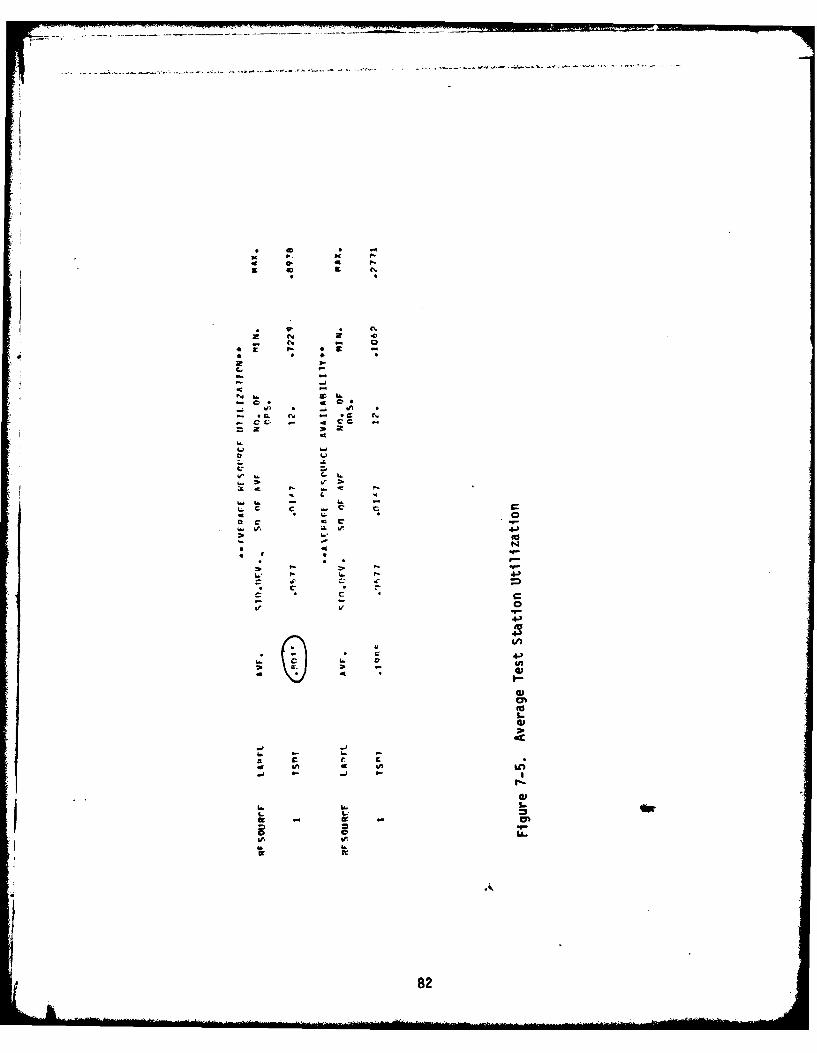
* * . -N P. N4 4 P.g ~ N

* * N2 N ~- N - 0

* ~ p.. * g -* *

2L

Nh.- ~ * 4 0 *- ./~ .- *C. N - *~ N- - 4 CC -

~ 24

Ufr U

J.v

- C. i.~., ~.

C - C -- L

I~ I~ - h. -L C C - C c C4 0o C

it Li. It .6**~0

- N* 4* r * -

L. 1 4)d

* C ** C *

- - 0It I -

4)04)In

I--I * 4)4 03

I-03

0I..03

-ph. -.a £ C* A 4 hi ~fl~i 9- ~J 9..

I-

03h.C. U lhrft - -

o 0 IL.WI It

I.ft

A

82

Comparison of Actual Versus Estimated Failures

Purpose of Analysis

Most Air Force resources that support aircraft are allocated based

upon an estimate of requirement in the support of flying operations.

Each avionic maintenance shop has a specific authorization level for

each resource assigned. These resources include test equipment mainten-

ance personnel, and spare LRUs. Individual shop supervisors have almost

no control over resource levels authorized but may request additional

authorizations upon identification of need and the ability to substan-

tiate the need.

Let's assume that a shop supervisor becomes aware of difficulty in

keeping up with the workload of the LRUs from a given aircraft system.

He knows that his authorizations of resources to support this system

are based on the required sortie rate and estimated mean failure rates.

He is also aware that the sortie rate flown in the recent past is within

the range used to determine his resource allocations. Every piece of

evidence suggests that the problem is due to aircraft failures occurring

more frequently than anticipated and the supervisor needs a method by

which this hypothesis may be tested.

Simulation with the system failure rate of the system of interest

set at the estimated mean sortie between maintenance action rate can

be accomplished. Output statistics such as those of figure 7-6 can

be used to compute an estimated mean number of LRU failures. Confi-

dence intervals about the mean can be established which define the

83

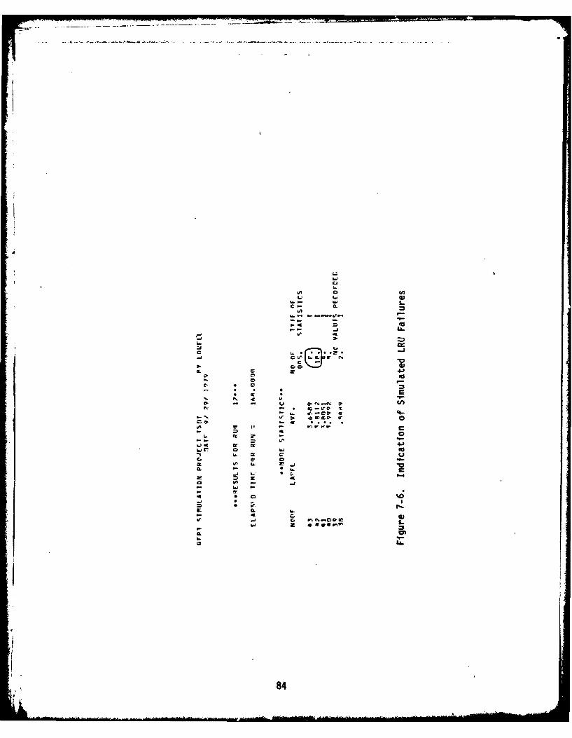
AL

II-l.IL 44

I--

jc fa,% 0CPICi z A .om

g.84

limits of rejection for the hypothesis that a sample mean is from the

distribution of the population (failure) mean. The mean for actual

realized failures can then be tested against the expected failure mean.

An Example Simulation and Results

The LRIJ failures of system 74B00 were extracted from the output

statistics of 12 simulation runs. The model simulated for this problem

had the MSBMA for the 74B00 system set at the rate used to determine

support requirements and the number of sorties flown were consistent

with original requirements. Computation of mean failures and 95 per-

cent confidence intervals about the mean are accomplished in table 7-2.

Results obtained in table 7-2 inlicate that if the mean X, of actual

failures is in the interval (22.14 X S 27.86) the supervisor can

state with 95 percent confidence that this mean number of failures

reflects the estimated mean failure rate. If X, the mean number of

failures realized does not fall in this interval he rejects the hypoth-

esis that the number of failures are representative of the estimated

failure rate.

Storage Requirements

Purpose of Analysis

A decision that is often overlooked in avionic maintenance shops

is that of allocating space for failed LPUs awaiting maintenance.

Temporary storage of most LRUs does not create a problem but there

are units such as RADAR antennas that may take several cubic feet of

85

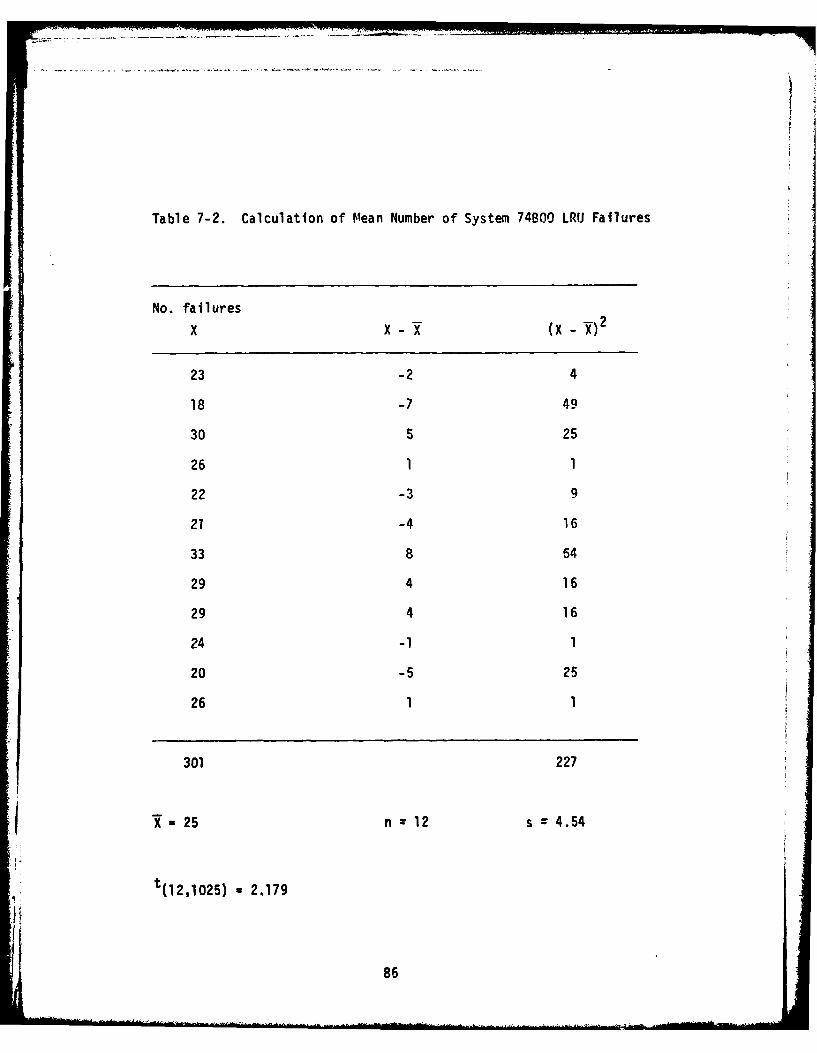
Table 7-2. Calculation of Mean Number of System 74800 LR(J Failures

No. failures

x x- (x Y 2

23 -2 4

18 -7 49

30 5 25

26 1 1

22 -3 9

21 -4 16

33 8 64

29 4 16

29 4 16

24 -1 1

20 -5 25

26 1 1

301 227

X 25 n 12 s 4.54

t( 12,1025) *2.179

86

storage space and if the average number of these units in the shop is

greater than one, lack of adequate storage facilities can create pro-

blems. For this reason management, in planning shop layout, must con-

sider the expected number of LRUs awaiting maintenance.

Method of Analysis

Q-GERT output summaries such as figure 7-7 provide a computed

average number of units in each queue and the maximum number ever in

each queue. The average number in the queue is time dependent and

therefore cannot be used for this particular decision. The maximum

number in the queue is the statistic one would use to determine storage

space requirements since it is most likely that this number is reached

predominatly over periods of operational shutdown such as nights and

weekends.

If one knows the dimensions of each LRU and the expected maximum

number of each LRI! awaiting maintenance, it is a simple multiplication

to arrive at the storage space required.

87

-- -----

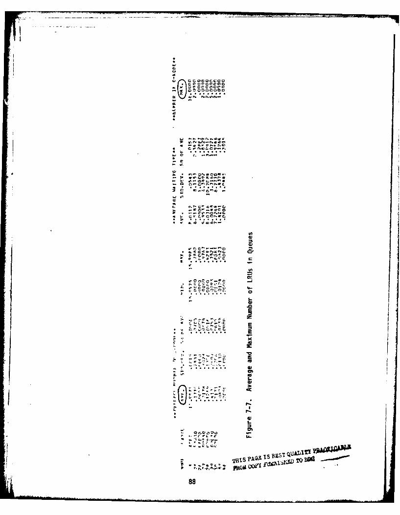
~OOO~C~Q1.1 C C~ OCOCCOC.

~z\.J UN NNUN.

&-J

LI ~ Np..0dIg~

-e ~ Vp-el NO4 OvN~CC0..F' 1

La. el * *******I.e C I.a-c- ~.

wa. *- ~

- ~* . . . . . . . . .

C ~-~'~C"'.Ce -

1.3 1J~

L .~@~CeLa. ... rc~P"...e#cC

* -- C~'--~oNr'JC.* 1. ~.L1 C~COt~.eC.* ~* el &.O .r(0~t--

InaJa)

r N* L~C~O.N~'C,

,~ ot~'~v'o- o~AwIQ.Cr

4. In=

o ~ C.0

.5. 1-a)

.05zS

C~cL~CC- * U

0

* - -. , - -.. .

~-j E0

a'0I-a,

.. '~3**-~~ * ~

I.-.

-I

C. I.-

* aiL

.5-

~ *~CLV IL.

88 -II----

VIII. CONCLUSIONS AND RECOMMENDATIOMS

Conclusions

Difficulties exist in the assessment of resource requirements

associated with the support of emerging weapon systems. Air Force

Test and Evaluation Center analysts require a method to analyze

critical questions concerning aircraft logistics support require-

ments. To be successful, the method must consider the relationship

between support resources and aircraft sortie generation. Management

alternatives and equipment design options relative to the support

system, must be readily evaluated. Evaluation results must be timely

and easy to communicate.

The objective of this report is to develop a Q-GERT model that

will meet AFTEC analysts' requirements. It has been shown that a

Q-GERT network can be used to describe the relationship between air-

craft sorties and avionic test station utilization. Networks such as

the one shown in chapter IV, provide graphic representation of the

system which gives management a clear picture of the overall support

process. Simulation of the Q-GERT model, demonstrated the ease in

which the network can be used to analyze various questions as posed

in chapters VI and VII. The analysis conducted in this report, demon-

strated the use of Q-GERT for decision analysis at Command and base

level. Model modifications were also accomplished to show the flex-

ibility of the model to analyze various "what if" questions.

89

Based on the results of Q-CERT networking and analysis accom-

plished and discussed in this report, it may be concluded that Q-GERT

analysis will satisfy AFTEC analysts' needs.

Recommendations

AFTEC plans to use Q-GERT analysis methods to assess F-16 avionic

* test station support should continue. Such an effort should focus on

the extension of the model to include manpower and spare LRUs as con-

straining resources. Upon completion of the F-16 evaluation, use of

Q-GERT should be considered for decision analysis at all levels within

the Air Force. The program should he made available to management so

that day to day decisions may be made using the same criteria as used

for resource allocation.

90

,O-A91 478 AIR FORCE INST OF TECH WRIGHT-PATTERSON AFB OH F/S 15/5AN ANALYSIS OF AIR FORCE AVIONIC TEST STATION UTILIZATION USING--ETCCW)DEC 79 J R LOWELL

UNCLASSIFIED AFIT-CI-71265T NL

2llfmlflfll

,hhhhohmhh

otis7

II - 1 .

MICROCP EOUINTS HR

BIBLIOGRAPHY

1. AFM 25-5. "Management Engineering Policies and Procedures."Washington: Department of the Air Force.

2. AFM 26-3. "Air Force Manpower Standards." Vol I: Aeneral.Washington: -Department of the Air Force.

3. AFM 66-1. "Maintenance Management" Vol I: Policy. Washington:Department of the Air Force.

4. ASD F-15/16 Manpower Study. HQ/USAF Directed Study Organized byLt Col Donald C. Tetmeyer. Wright-Patterson Air Force Base, Ohio:Headquarters, Aeronautical Systems Division. October 1975.

5. Branson M.H., and B. Shah, "On GERT Modeling of a Class of FiniteQueueing Processes," AIIE Transactions, Vol 4, No. 1, 1972, pp 43-48.

6. Chad, Lincoln L., "Statistics: Methods and Analysis," Mcrraw-HillInc., New York, 1969.

7. Davis, E.W., "Project Scheduling tnder Resource Constraints-HistoricalReview and Categorization of Procedures" AIIE Transactions, Vol 5,No. 4, 1973, pp 297-313.

8. DeGovanni, George and Donald M. nouglas, "Estimation of F-15 Peace-time Maintenance Manpower Requirements Using the Logistics CompositeModel," Master's Thesis, Air Force Institute of Technology, 1976.

9. Donovan, James G., "Test Station Modeling and Analysis Using aQ-GERT Network," an unpublished paper, Headquarters Air Force Testand Evaluation Center, Kirtland Air Force Base, New Mexico, 1979.

10. Drake, William F., III, Rolland R. Fisher, and John R. Younger,"Logistics Composite Model Users Reference Aulde," AFLC Report70-1, Wright-Patterson Air Force Base, Ohio, 1970.

11. Drake, William F., III, "Logistics Composite Model U1sers ReferenceGuide Update" AFLC/ADDR Report 74-1, Wright-Patterson Air Force Base,Ohio, 1974.

12. Elmaghraby, S.E., "An Algebra for the Analysis of Generalized ActivityNetworks," Management Science, Vol 10, '.o. 3, 1964, pp 494-514.

13. Emshoff, J.R., and R.L. Sisson, "nesign and Use of Computer SimulationModels, The MacMillan Company, New York, 1970.

91

14. Grant, Eugene I., and Richard S. Leavenworth, "Statistical QualityControl," McGraw-Hill Book Company, New York, 1972.

15. Gunkel, Richard A., Study of Air Force Aircraft Maintenance TaskTimes, unpublished report, Headquarters Tactical Air Command,Langley Air Force Base, Virginia, 1974.

16. Hogg, Gary L., et al., "GERTS QR: A model for Multi-Resource Con-strainted Queueing Systems Part I: Concepts, Notation, andExamples," Allie Transactions Vol 7, No. 2, 1975, pp 89-99.

17. Hogg, Gary L., et al., "GERTS QR: A Model for Multi-Resource Con-strainted Queueing Systems Part II: An Analysis of ParallelChannel, Dual-Resource Constrained Oueueing Systems with HomogeneousResources," Alle Transactions, Vol 7, No. 2, 1975, pp 100-109.

18. HQ/AFTEC, "Cost of Ownership and Handbook," Air Force Test andEvaluation Center, Kirtland Air Force Base, New Mexico, (May 1976).

19. HQ/AFTEC, "F-16 FOT & E Phase II Suitability Test Plan - Annex E,"Air Force Test and Evaluation Center, Kirtland Air Force Base, NewMexico, (Sept 1978)

20. HQ/AFTEC, F-16 LCOM Study Plan Series, Air Force Test EvaluationCenter, Kirtland Air Force Base, New Mexico, undated.

\ 21. Morris, William T., "Decision Analysis," Grid Inc., Columbus, Ohio,1977.

2" Mortenson, Robert E., "R, M, and Logistics Simulations Using Q-GERT,"paper to be presented at the 1980 proceedings annual reliability andmaintenance ability symposium, Headquarters Air Force Test and Eval-

I uation Center, Kirtland Air Force Base, New Mexico, 1979.

23. Musson, Thomas A., personal letter "Engineering Report UtilizingQ-GERT on F-16 AIS," Air Force Test and Evaluation Center, KirtlandAir Force Base, New frexico, (Sept 1979).

24. Pritsker, A. Alan B., "Modeling and Analysis Using .-GERT Networks,"John Wiley & Sons, New York, 1979.

25. Pritsker A.A.B. and R.R. Burgess, "The GERT Simulation Programs-GERTS III, GERTS IIIQ, GERTS IIIC AID GERTS IIIR," NASA/ERC ContractNAS-12-2113, Virginia Polytechnic Institute, (May 1970).

26. Pritsker, A.A.B., and W.14. Happ, "GERT: Graphical Evaluation andReview Technique: Part I - Development," The Journal of IndustrialEngineering, 17, 5 (May 1966).

92

27. Tetmeyer, Donald C., and Sharon R. Nichols, "Simulation MaintenanceManning for New Weapon Systems: Maintenance Data Analysis Programs,"AFHRL-TR-74-97(111). Brooks Air Force Base, Texas, (May 1974).

28. Whitehouse, Gary E., "Systems Analysis and Design Using NetworkTechniques," Printice-Hall Inc., Englewood Cliffs, New Jersey, 1973.

29. Widenhouse, William C., and William E. Romans, "A Forecasting Tech-nique for Operational Reliability (MTF) and Maintenance (M'H/FH),"ASD/TR-77-28, Aeronautical Systems Division, Wright-Patterson AirForce Base, Ohio, (May 1977).

I 9

APPEN"IX A

Pata Input Description

This appendix includes the input cards required for simulation

of the model design of chapter IV. Computer printout of the input

data for a successful simulation is presented to aid the interested

reader in obtaining a more thorough understanding of this report,

In subsequent pages, the following information is presented:

1. A sequentially numbered list of the input cards used to

describe the network model. Comments are printed to the right of

selected card inputs to clarity the intended purpose or function of

the input.

2. Network description printout which details all Q-SEPT func-

tions and the characteristics of each function used in this simulation

follows the input cards.

3. Finally, the input cards are again presented in the form that

would include diagnostic messages to aid in simulation debugging if

system errors were present. The only messages in this example are at

the end of the input, and they merely show intended parameter set usage

and state that no errors were detected in the input.

I9

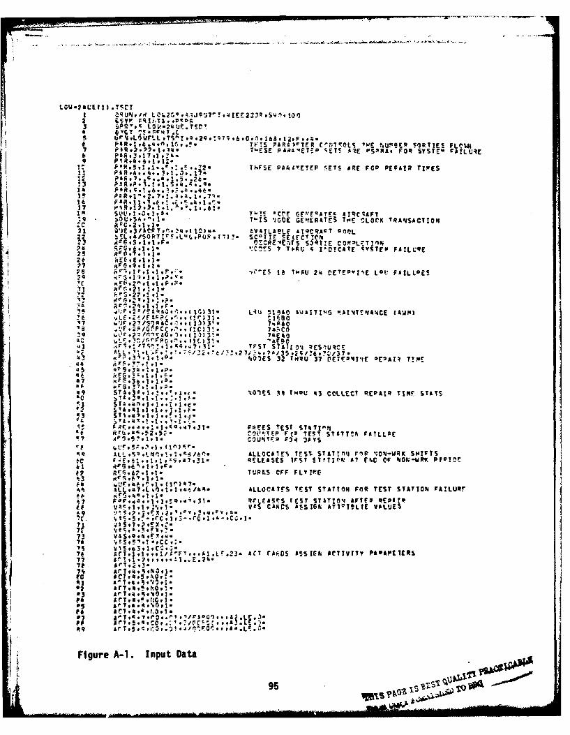
E ST?, AR I Js.IPC *3 daPiVTe LW.?giIJ!F.TS{C!

# PAR gee .4 n I If 9 Tv S P*A&'TE R c r.,TqOLS IIJ %.U~wEP SORTIES PLCUA7 01 AR 92v,)29 14 TA-SE P A?&ETr-v SETS 4.4E OISM14*. FOR SYSTEM4 r5!LU4E

b PAR,3,1791,ss49 P~*.vv

ThFSE PARIL'ETEF SETS ARE FOP PEFAIR TIVES

IN S(U.1.3.1.*. T'-!S PCIr GF.E EATEC A1RC;AFTI9 ~ U5A'1 Ti-1S -JOE GE-IERAT!E Ts NE LOIK TfA4SACTIONd

22 Q'JE93/A1FTv,-.2s.Ia). fV*ILAFLE £TQCRAcT P~I-2? b-L4SR~!#1r9~- SC0 TTE SELrCII10%

ZG51lF 3:C"RE ENjS S39T!E COMOLS-Trnaipit "FG96.191..C T ES 7 TO.Ri S I'OYCATE iYTE F5!LtQE

4 25 Ret:,70i.1.2f, R-E.E9101.

2" r 1 , 91 11 'E S le INF'U 2'. CETrOv1lE LOU FAILL0 ES

if, r,21/.C,,I)1 t 1 CO

?2 C' L.F - 71-%3 to r.~E 32 "149 17 OE-~4 ,'I VP

ar', TS TTI 1 ZSTI R

47 .4. 1 1 TU t. IF I I IP'b F mi. !8*' $1 0 P3)7

AL49.~.,O/~ STLOCTS 14 TU4 STAION RPAI TEST STA YSFALR

i~a! C3S STITIO', AFTER 9E"AY*'C7A.4 . 1.,!

9 AS: @4; 9n9 ' I y ;014 31FIES TE~ST AST4IAAIL1LT LE

73 m r, 9 1 0 1 1

vact.1.!'1,,1.'.,1L.3 £CT CAROS ASSIGN A STVITE VSALUECS

777e D?....O:

P4 A Tt elA ! I tO,1.

FiueA-1. Input Data

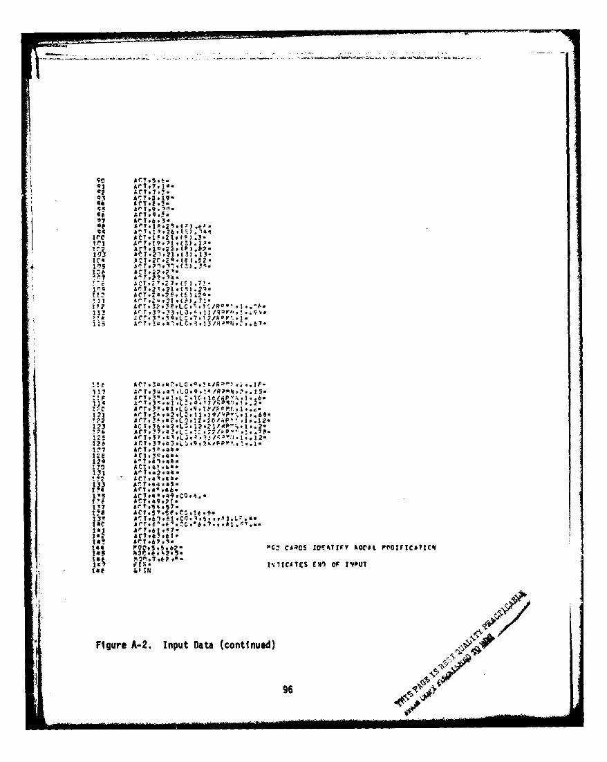
93 ArT93 9190

ire

I9 T 97 - 1 .6*4 .19-

We £T.I0.21,4P .3-.

C03 *C1. 21 v219( 3 1 .13*".4 CvCqv2."

:!L% OTt22#21

i* .1CTv2'.?7. (2.7'r It! AfT t2 121 9 R) .21

U? ACT* 31.93PvLQAI '/R011' # ..- 41-

; C! . , 19 'L ',1t.. 71A P * 6A -29419L 3I M 9 V .l2

'2 Ar T9;4 ,L..2/P ($I I .

F 17%k 9L: 91C--v. 6-

119 AOT,3= l -4 99 ?R :.-92

!P2

1 3 A CT 9 #1 t- 1

1:%7 ACT.*32944

I'S Iri7a'C440~.12 ,041#447.

13 ACT#!'.9#,0,l

t33 ArCT #* # 052 14? AT.atah

13a e 61 AI*C-9f

I ACT 0966

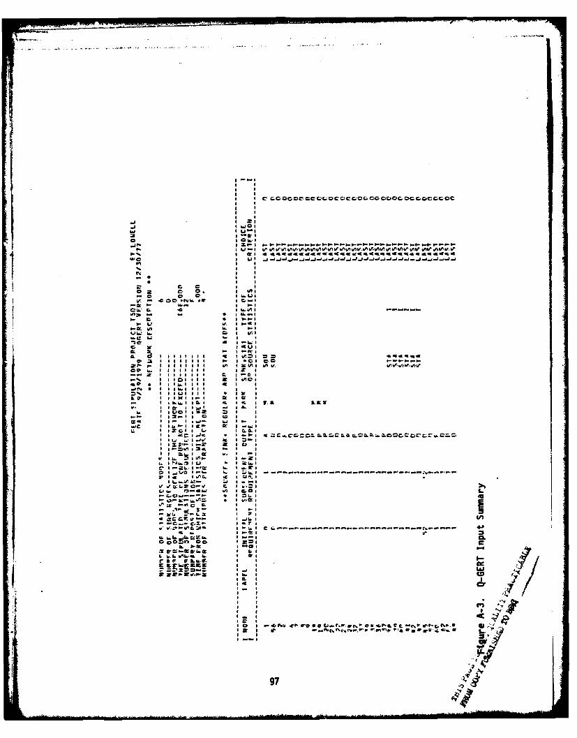
I Zi

0 . .. :

.9- ,ll

. * IN

I I

-. Is I ,-I,I II O

000.

- :s I 0- s - - s - - s -

,-,.o s'l uI

we I mI

Q I

.! t. I Iv I LII I A I. I.

,, N.I s I u - I /I I V

3-- n IV I-. I

i fr * I tII I I II 4 II I11 lm-m.,m m m m m m m~l.m lll.+~mm-m *+

S IIia II * I I

I3rt -Ill; w I.r g LI 7- I

-~ - -h -ws - ---------- 4

* L. L .o..,.I,-_ o

*o eh o - I ;

9 1 . *V" - I" . l

I. b.u 0't-l 6.

o"In I -I. I.,.I . Ii--

r a 0 cr I UI

10 ,f,, .,,, Co.+ .a 0 tj t... ;cf. - G. aI +L.I. 0

0i.' 0 I

~"2 ~C 97

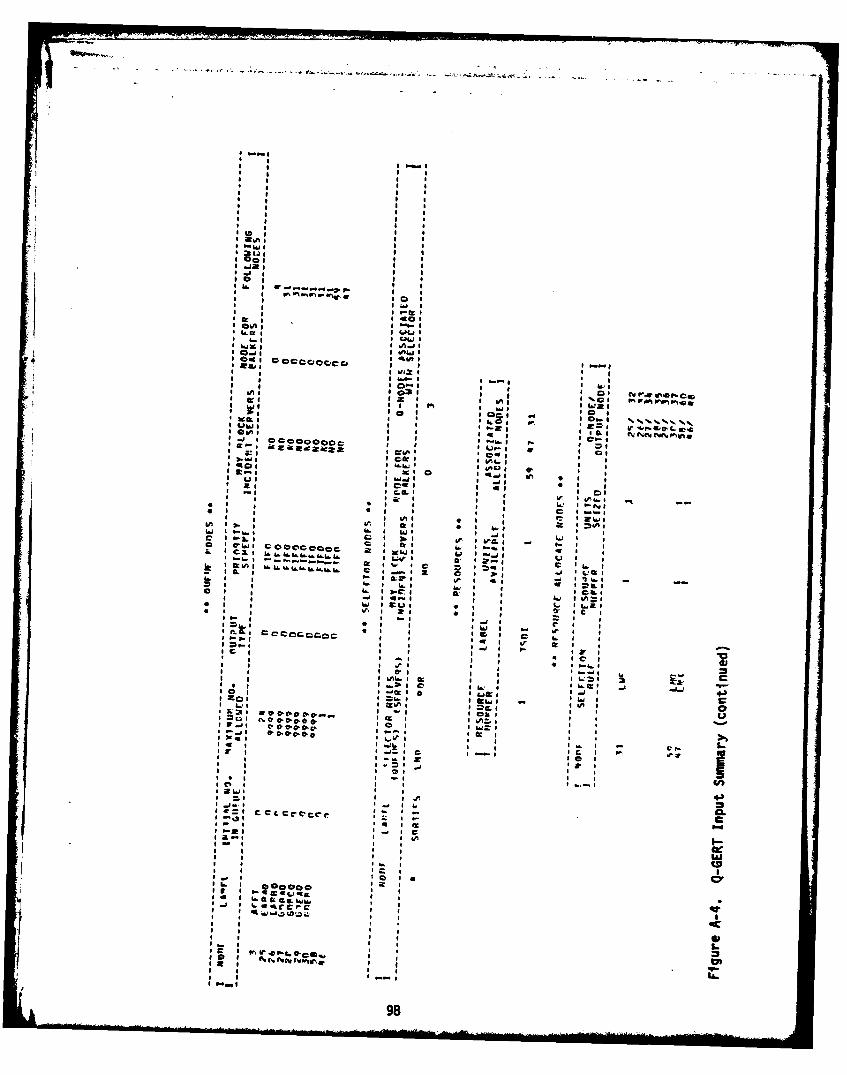
*Caw*X InS

* 4011"1a L4S A

S~ I

id aa aa

a m

SJ I

a a. I

IA:CR aI40

kA OrA

C~: ~Sr Sore

S 5~ a S -S-S -~RE

S.1 Ar I

OR* ~ 5s

;.g I~w o. ..4 aF~aa

S II S1

a CL- ,S~- I

cc S v.4 S. S-5 : m Sb

S a - SE~ a.., gI98

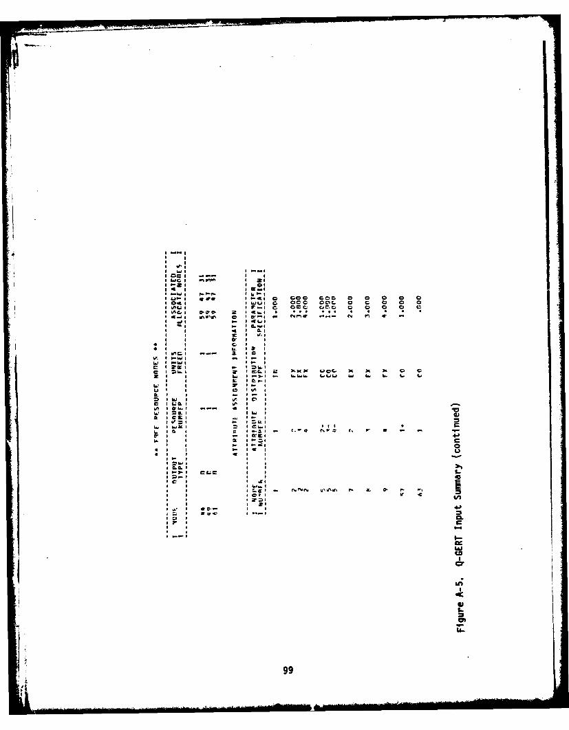
I Lo :c O O

it IP 2 c 9s

I W.C Im CY n A

4IL

rur hU, w%-r fir hILI*-I~ ~~~~ -* ~ i C C C C C 0 0 0 C C

* 01 ~ ,g C C 0L 0 C C

*r~i CCC c.Cc a C C C

Ihj~I ~O~ 2 44 * .99

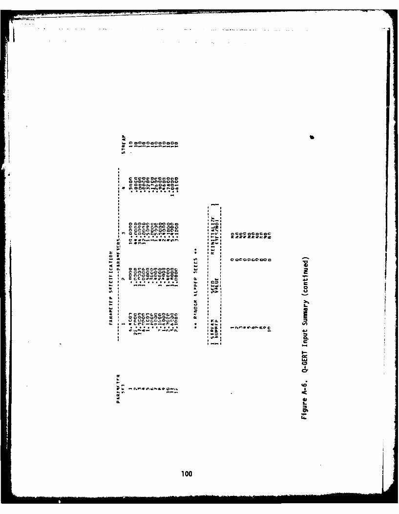
a- COoQCV.o" CO

a ec~eccccca 0 -CCL U0C0CIa eoeincena-

aX I

I~6 0C ococciacc a-c

0coer-00cco~cc 61 1a com~orcar0u0-w0 wl I~a ecce

&~~~~~.6 1. cN--.U W .P1a-

&L aa . aCs I

000. ocC coecc a-a- a C~c~c.co~co aa

a.. CC~'OO CCCC O I I- a ccc a~p..wara w~ 0. a-a- I............*... a-a06

a-or ~ - ~ .. 0 a.a

r6aa maa

C6 ~aa I .

I 400

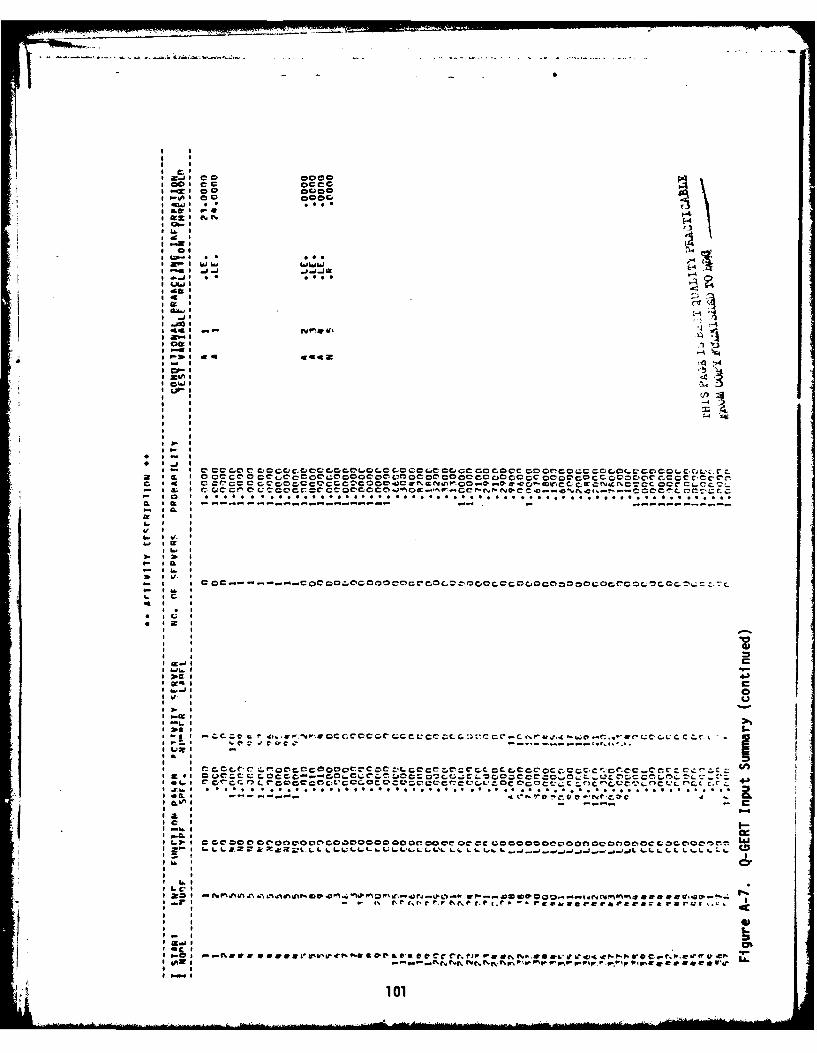
aS co 00CP Ci oC 0000

a x ow 0 O

W-a0000aWaX m0 .00

-I a C.).0 *amaaa

.9 44i --

* Of I ) :4

* M4a

C, 0 £44 C. Ml ,Q0QQC ,r %L -0C0c0ce0r cc -C0QC 0 c0L .C lc i ,0CCLaCO-avDc otv ccC coz 0 0c OLC coccccrCCcCCC l

ac ocz0eVn . Cc N fcac -

I I

* f a

I- a- -:

cae ,Q ~ - c) coc Zccc CC co 0cec-cc0c 0,.c rc 0c rc c-OCC c~~c oc C -c. zC.c Z.Z

c- Q M L c- cc'o Q C CCC'r-er CC W LOQCC-'C - C rCL*C e'' N~~c-C n n .a-- C WL rlrC. 4

a. a.

r a Iti.l a- c O Q

&~ISO.

aimaa c0 -aa a w I ~ l r e - - - - a 6 4 . c ~ . r o W l o . r r . r i l - c - - . s * - ~ r c f 0-V, aN h.e a&rPP ~ , Vr .pw~r" n rv0A rVj 1r

~ a g10a

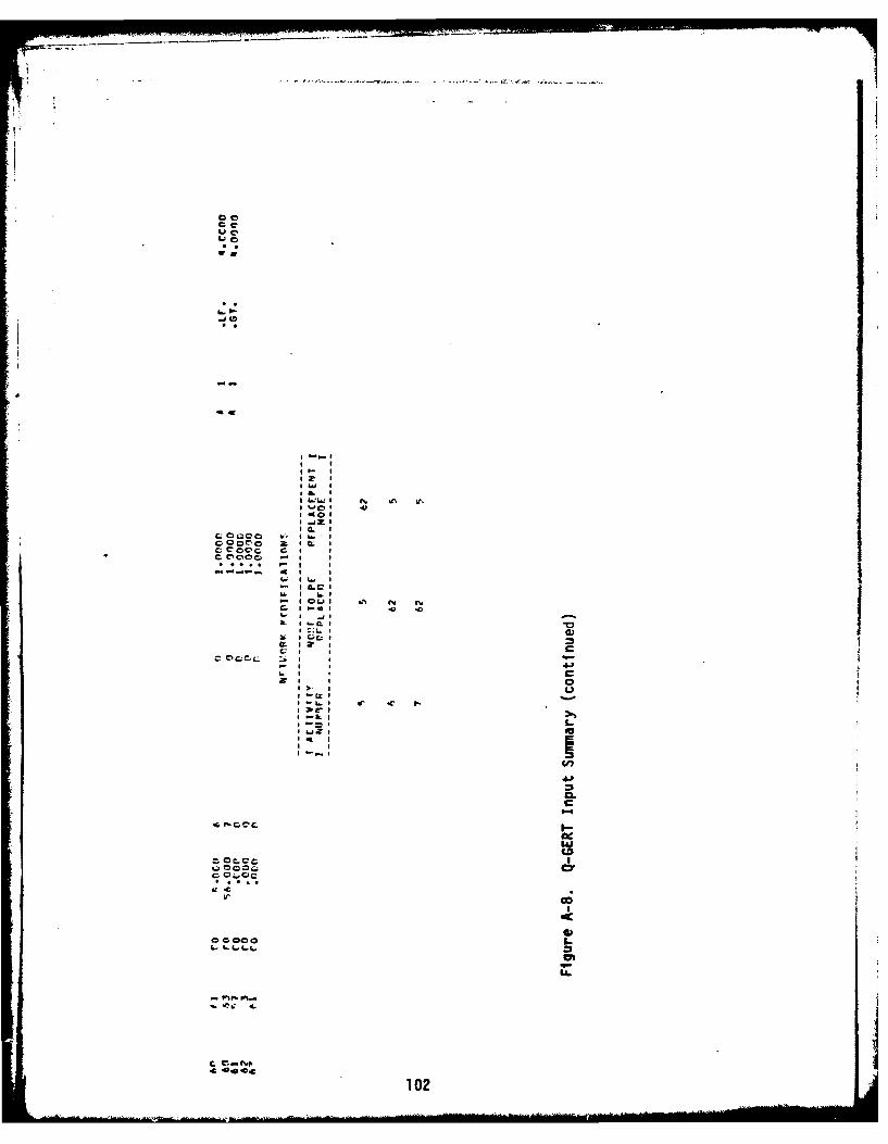
LaC

a. a

coor- c

* Wz I

IC.L

.G . OQ C *-.

sCCCC* *. -

cocoa

b.L

* ~102

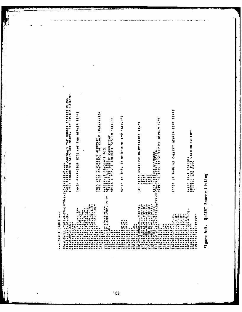
C, ~-- j I..C

WG - -

.T a4 'W-

C,. IAj V L. - 44. L. .1j. b a- 4..

Ir or. C . ccJ W N - I0u. SK - 6.i. a C

L. 4. Cw Z 4 r ~ -W C. I

wx LI .V -h~ 1C. mrWJ*

'c U K1 -i -C m4.c1r j'f 42-. L; 1.

*~0 tr Lt KK L t L- w-- a: -. *a a.~ ;0

LLZ V

.C .4 . .. .

*40. .. .1. . . ... -

*IL. U t- . ,~. C

C~~ .. . .Z .Q . . .. . .

L

1030

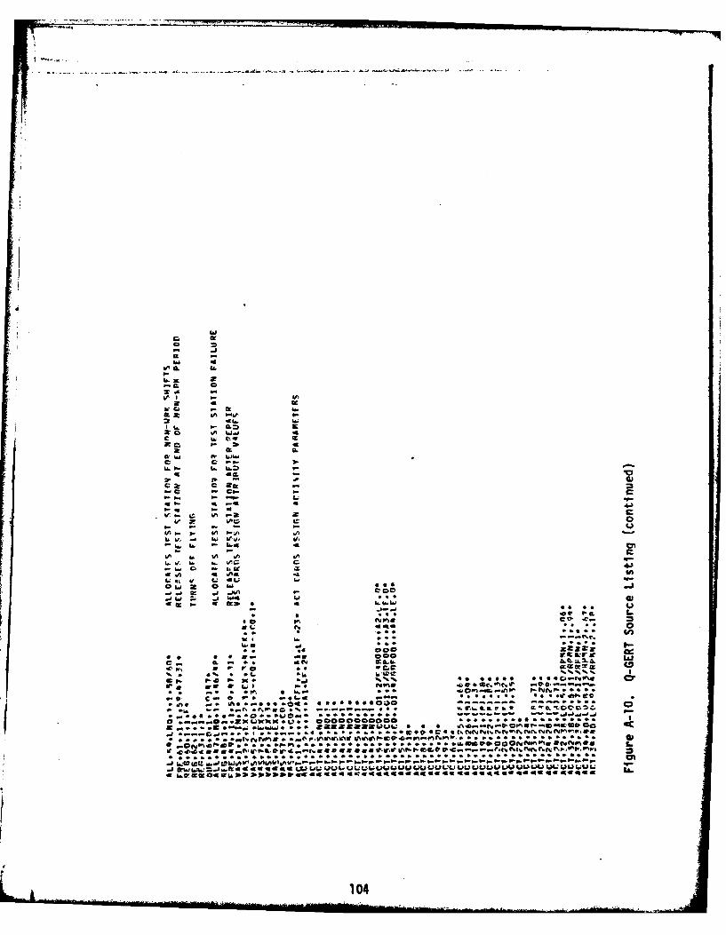
Q or

W --

U~. 44.

4 44

r OL caa

.4 u -14.

.J 1 -0 010

P. 61 =1 - ,OC 4 P

4 .

a~ anD-.

WIt a. a.& a

.an I. S, Ia

C ~ If 0 4 1 4

.~ . . . .. . v .- CO...O

*,a .a. 9aI6

S C 4aNM* 104

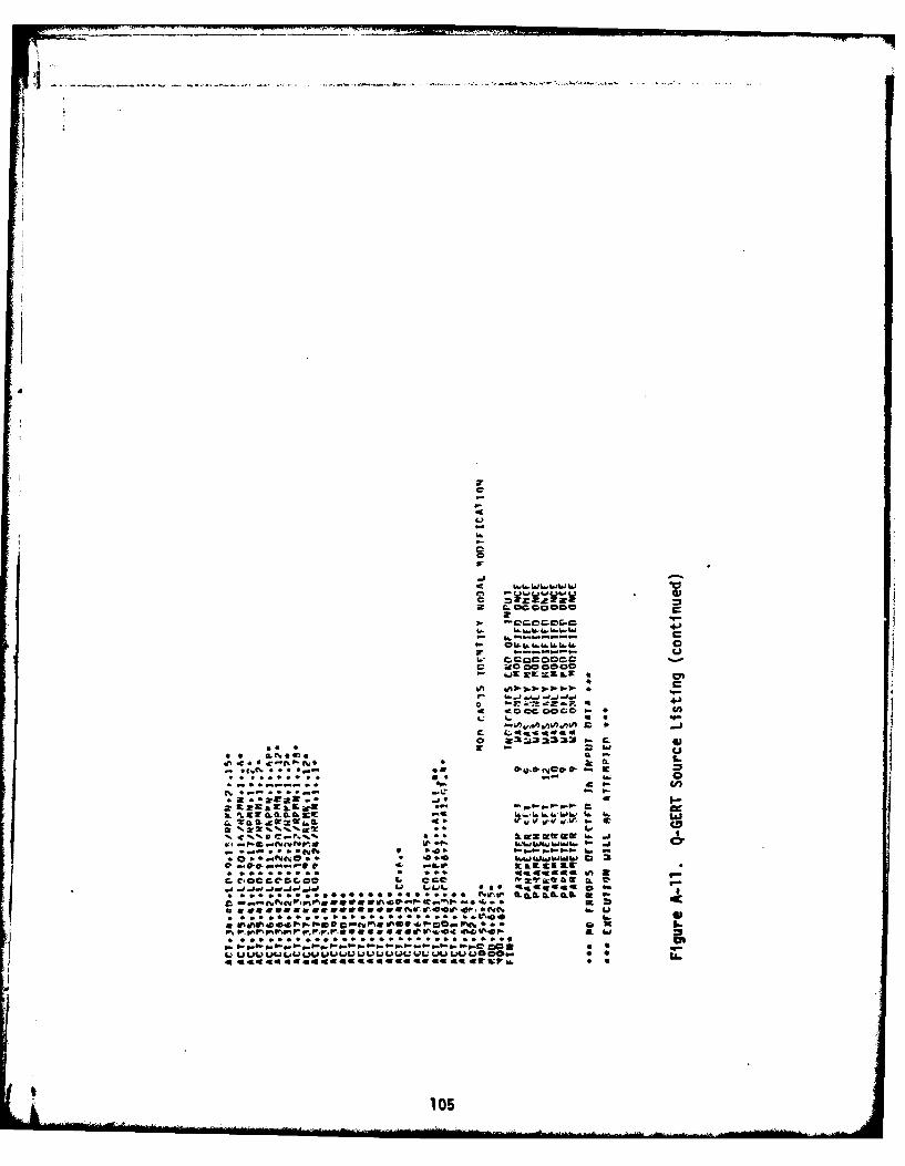
occ P. W .~

!V !:

tCo 0

UW

6 l6lWLWW "61c

am am* "

105

APPENDIX B

Summary Report Description

This appendix includes an example Q-GERT summary report. The

summary presented is for a simulation of the model design of chapter

IV for 168 hours (one week) with a requirement of 20 sorties flown

per day.

Most of the data items in the report are self explanatory but a

discussion of selected element headings is included. nata elements

that are discussed havea number next to them that corresponds to the

following:

1. ***RESULTS FOR RUN I***: identifies the run number for which

the subsequent statistics were collected,

2. ELAPSE)Y TIME FOR RUM! = ; indicates the simulation time units

required to complete the run;

3. **NODE STATISTICS**; provides data collected at statistics

nodes. The average column for each node may be a release time, a delay

time, or an interval of time depending on the type statistic requested.

The number of observations column indicates the number of node releases

that occurred during the simulation run.

4. **JflUt3ER IN Q-NOnE** and **WAITING TIME IN QUE!IE** are sta-

tistics associated with the number of transactions that must wait in the

queue and the time spent in waiting. The average number in the queue is

a time weighted statistic and the maximum number in the queue is absolute.

106

5. NODE and TRANSACTION PASSAGES ; list the node numbers and

indicate the number of releases of each node during simulation.

6. **FINAL RESULTS FOR 12 SIMULATIONS**; is an accumulation of

the statistics collected in each simulation run. The output format

is similar to that of the individual run statistics but the averages

are computed on the average from each simulation run. The observation

columns reflect the number of simulation runs included in the compu-

tations.

7. STAT HISTOGRAMS FOR NODE 43; provides a histogram of the sta-

tistics collected at node-43. OBSV FREQ is the number of observations

in the range of the cell defined in the column at the far right. RELA

and C1!ML FREQ are the relative and cumulative frequencies of the obser-

vations. These frequency statistics may be used to estimate the proba-

bility distribution of the variable measured by the statistics node.

107

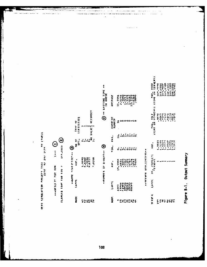
). CL C a-- L ot- 00 r, C'C,C'

.A a C Lf 1,4 C 0

co ar,.. *L .C * *

IDn" 4 r f-4.P90U

- . 3- 0

3w 41t

C~c a.. CC,~C'Z

m .0 lzC.-NOPa.W. Ow :tw "', Cg

0t A0a C.CCLi xc

41 .r a.*.* . -

8. COX0-a 4 0-N ;C .46 0 no-a&C L44 P

a a v. mtkCm m Lli a f

o riq 2 ***.10*

9.- 0Mf-

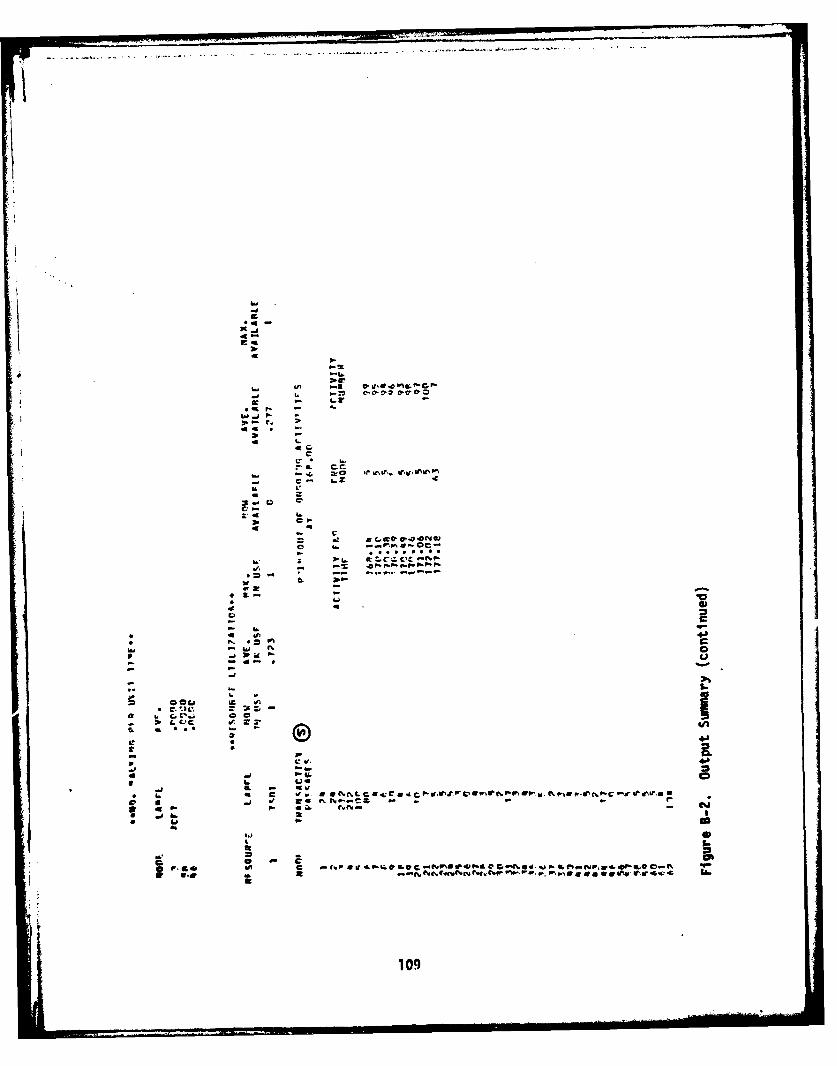
h2.

I- J

;t 4x -

A44

V. L.

.- LI r-9,

4.

c 4A

C .%

201 9

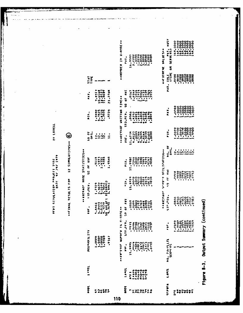
C, C4- no oc j o

a~occoc.ccoo

aa 0000.0o cc,-L C; 90000C.0

r.4 i. c6 . *.. L~rlq P I

3: a. 47 0rt

y It* x ~ cecoeoco

cob W~ v- c*Cl0000. -0 v- e IL c0 0 0

P. #- wN 40 (1% 4 . .1 !00 0' ow-We r-. % a- , 0 P f~V 040 6 * C . 0 0 . 0

a~c 0 QruL 420 cc

L, "P zo *: QNCC0"cC -

.9 - 0 . -Cf 9%C.*.4.*.*

owo

O*(Q CC

SCOvoemV. C.cr vC-C.crAL~U~ c Q 04715 C *. ...

C, Cr* *of. or

j ci

p. op P.****. C. * *. C-

-,r t.0

r-0c 3;4 p A00 P, Z.t. 0e'.Ne.0

21 *% ** -*ff C t-~.Q - I40 tw 0 41 f~Ep

p. -. c C

TM t 1 4. 0000 f4..t .0 c a.rov raf

o -4 4..

* C. am

C. .I...#S Pw a4P00 U.40

a~ ~ 168~u IL~**

U'Ch11W0

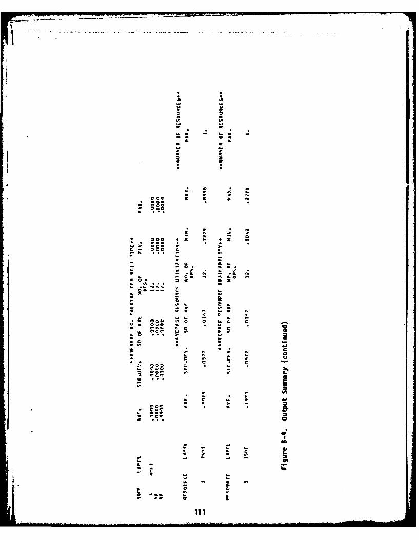
InILcooh

C, C

A. a

E . w ;& ir

*1 wD. c

ca

v o. 4 tcC cca f* 00D

31 L 1

4 0LO£ *

* L

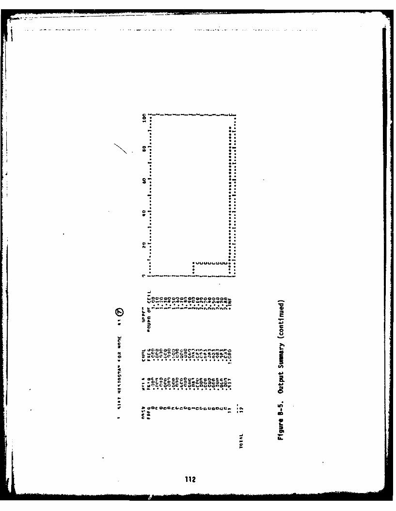
0e

- .

* 0.

* 0*

* 6*0-* * 0e

* 0e* 0s* 0.

- 0-* 0e

. 0** 0*

0-4b 0.

* 0.

* 0.

* p.* 0** 0** 0*

0~ 0-w * 0*

* 0** 0** 0*

* 4.* p.* 0** 0*

0~0*

* 0** 0.* 0*

0~* OUUUULDUUU. ** 0 0.* 0 0.* 0

h~OOC@O0C0O@OO000§0h.

C Ic NNPC.NNNNNO(9 I~c 30. C

w 43o Ca 0U

WC.C-

~ Uo ~ Ip

C.-

C E @C~OC~CCCCOCC!p. a-. - ~Ic ~

- t- **********p*.*.*.*.* 0T

*- I~ CIOC 000C-&CCDC..CC~OI0CcC...

- I-eaCI.. S

S.=U'

*

C.

112

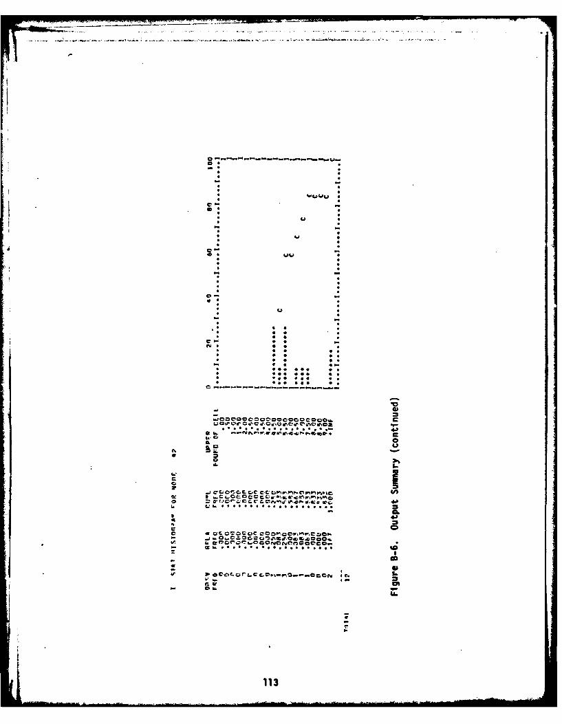
- ~ ~g.-~. -

0*- .

*S S

* SS

* ~UUUaC- -U~ SI. LI

S S

S SS S

4 -4 * S

* S* S

S SS S* S* S

* SS S

* U SS S

* S* S S S* S * S* S * S

C.- * . -.N 5 0 *

* S * OS* 0 0 5.* 5 0 5.

- S S* @00 400 *S* 405 400 05* 550 OSS 0.* 000 *45 0.

C

V- @1

0000C00000000c00§i. C

b 1 ~ CC

N*

o'a. I.

I..'CC

4 J=C

*a. ~

- m- *SSSSSSS*..S..*..a.s

0'It.

a" -fLit

- Cli,

S.

113

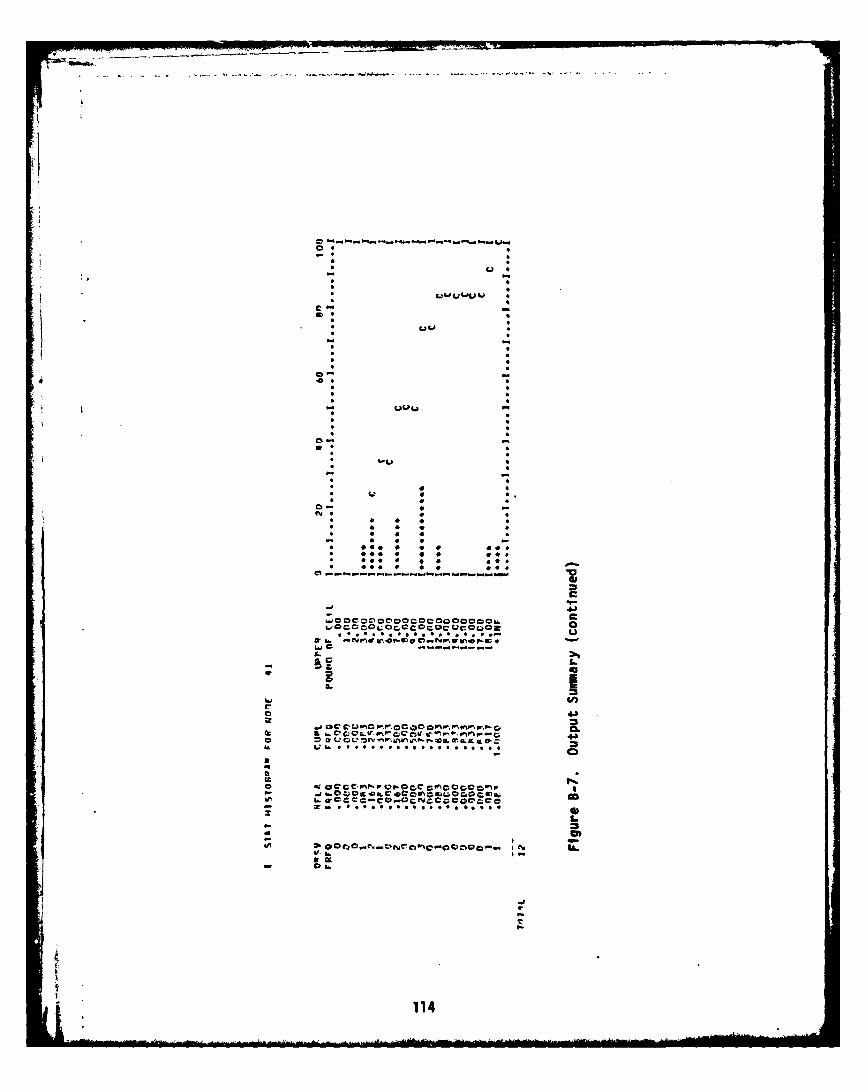
4 -0

----- -- a----

a.

-s a LScC n-PoI ot

Cw--SL

4 114

. .

- .

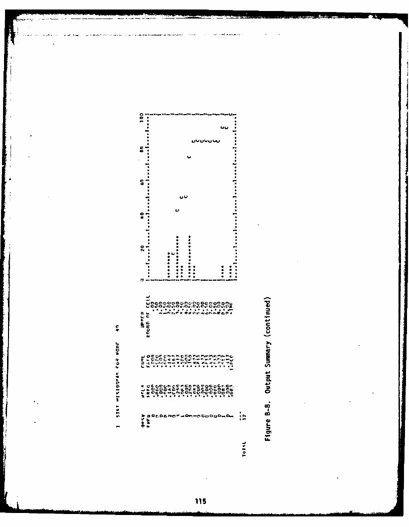
. .u ..

* UI-u(-,'Ju1

It0

C-4J

LI 0 i c C"i c :.C

* 0

* U .0 0 j

*115

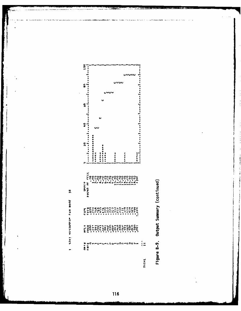
-----o - - - - -

0 0

C-

44.

v - -

*4 )

* Q

* 4 * JC- 4 INe 4c4

IL 4 4

* 4 &

* 4 116

BIOGRAPHICAL SKETCH

James Russell Lowell was born April 9, 1942 in Minneapolis,

Minnesota. He graduated from Corona High School, Corona, California

in 1960 and entered the USAF. Attending classes at the University of

Arizona and the University of Maryland, he became eligible for and

was selected to participate in the Air Force Airmans Education and

Commissioning Program. He completed his Bachelor of Science negree

at New Mexico State University in 1973 and received his commission

as a second lieutenant in the United States Air Force.

In August 1978, Captain Lowell entered Arizona State University,

sponsored by the Air Force Institute of Technology, to pursue a

M4asters of Science Degree in Engineering.

Captain Lowell is a member of Alpha Pi Mu (industrial engineer-

ing honor society) and the American Institute of Industrial Engineers -

Student Chapter.

117