Embed Size (px)
DESCRIPTION
Backward Facing Step Numerical Investigation
Citation preview
J. Fluid Mech. (1997), vol. 330, pp. 349–374
Copyright c© 1997 Cambridge University Press
349
Direct numerical simulation of turbulent flowover a backward-facing step
By H U N G L E1, P A R V I Z M O I N1 AND J O H N K I M2
1Department of Mechanical Engineering, Stanford University, Stanford, CA 94305, USA2Department of Mechanical, Aerospace and Nuclear Engineering, University of California,
Los Angeles, Los Angeles, CA 90024, USA
(Received 14 March 1996 and in revised form 3 September 1996)
Turbulent flow over a backward-facing step is studied by direct numerical solution ofthe Navier–Stokes equations. The simulation was conducted at a Reynolds numberof 5100 based on the step height h and inlet free-stream velocity, and an expansionratio of 1.20. Temporal behaviour of spanwise-averaged pressure fluctuation contoursand reattachment length show evidence of an approximate periodic behaviour ofthe free shear layer with a Strouhal number of 0.06. The instantaneous velocityfields indicate that the reattachment location varies in the spanwise direction, andoscillates about a mean value of 6.28h. Statistical results show excellent agreementwith experimental data by Jovic & Driver (1994). Of interest are two observationsnot previously reported for the backward-facing step flow: (a) at the relatively lowReynolds number considered, large negative skin friction is seen in the recirculationregion; the peak |Cf | is about 2.5 times the value measured in experiments at highReynolds numbers; (b) the velocity profiles in the recovery region fall below theuniversal log-law. The deviation of the velocity profile from the log-law indicatesthat the turbulent boundary layer is not fully recovered at 20 step heights behind theseparation.
The budgets of all Reynolds stress components have been computed. The turbulentkinetic energy budget in the recirculation region is similar to that of a turbulent mixinglayer. The turbulent transport term makes a significant contribution to the budgetand the peak dissipation is about 60% of the peak production. The velocity–pressuregradient correlation and viscous diffusion are negligible in the shear layer, but bothare significant in the near-wall region. This trend is seen throughout the recirculationand reattachment region. In the recovery region, the budgets show that effects of thefree shear layer are still present.
1. IntroductionSeparation and reattachment of turbulent flows occur in many practical engineering
applications, both in internal flow systems such as diffusers, combustors and channelswith sudden expansions, and in external flows like those around airfoils and buildings.In these situations, the flow experiences an adverse pressure gradient, i.e. the pressureincreases in the direction of the flow, which causes the boundary layer to separatefrom the solid surface. The flow subsequently reattaches downstream forming arecirculation bubble. Among the flow geometries used for the studies of separated
350 H. Le, P. Moin and J. Kim
flows, the most frequently selected is the backward-facing step. Considerable workhas been carried out on this flow due to its geometrical simplicity.
The effects of expansion ratio (ER) on the reattachment length were studied byKuehn (1980), Durst & Tropea (1981), Otugen (1991), and Ra & Chang (1990). Thereattachment length was found to increased with ER in these studies. Armaly et al.(1983) studied the effect of Reynolds number on the reattachment length, Xr . Theyfound that Xr increased with Reynolds number up to Re ≈ 1200 (Reynolds numberbased on step height h and inlet free-stream velocity U0), then decreased in thetransitional range 1200 < Re < 6600, and remained relatively constant when the flowbecame fully turbulent at Re > 6600. Their findings agreed well with experimentsby Durst & Tropea (1981) and Sinha, Gupta & Oberai (1981). Other parametersaffecting Xr were also investigated: upstream boundary layer profile (Adams, Johnston& Eaton 1984), inlet turbulence intensity (Isomoto & Honami 1989), and downstreamduct angle (Westphal, Johnston & Eaton 1984).
Eaton & Johnston (1980), Westphal et al. (1984), Adams & Johnston (1985), andDriver & Seegmiller (1985) all measured the skin friction coefficient, Cf , on the stepwall. Although there is a large variation in Reynolds number and expansion ratioamong these experiments, all reported a high level of |Cf | in the recirculation region.The present study showed that the peak value of |Cf | can be significantly higher at lowReynolds numbers. This finding prompted a companion experimental investigationat the same Reynolds number and expansion ratio as the present numerical study(Jovic & Driver 1994).
Investigations of the flow velocity profiles and turbulence intensities in the recoveryregion were conducted by Bradshaw & Wong (1972), Kim, Kline & Johnston (1978),Westphal et al. (1984), and Adams et al. (1984). These experiments showed that, eventhough the mean streamwise velocity profiles were not fully recovered at more than50 step heights behind the separation, a full recovery of the log-law profile near thewall was attained as early as 6 step heights after the reattachment.
Several numerical simulations of the backward-facing step flow were also conducted,but largely confined to two-dimensional calculations (Armaly et al. 1983; Durst &Pereira 1988; Kaiktsis, Karniadakis & Orszag 1991). Three-dimensional calculationswere also performed by Kaiktsis et al. (1991) and by Friedrich & Arnal (1990) usingthe large-eddy simulation technique. The present direct simulation is the most detailedand extensive calculation of turbulent flow over a backward-facing step. It providessome insight into the unsteady characteristics of this flow as well as a databasefor turbulence modelling, containing up to third-order statistics and Reynolds stressbudgets at all locations in the flow field.
2. Method2.1. Computational domain
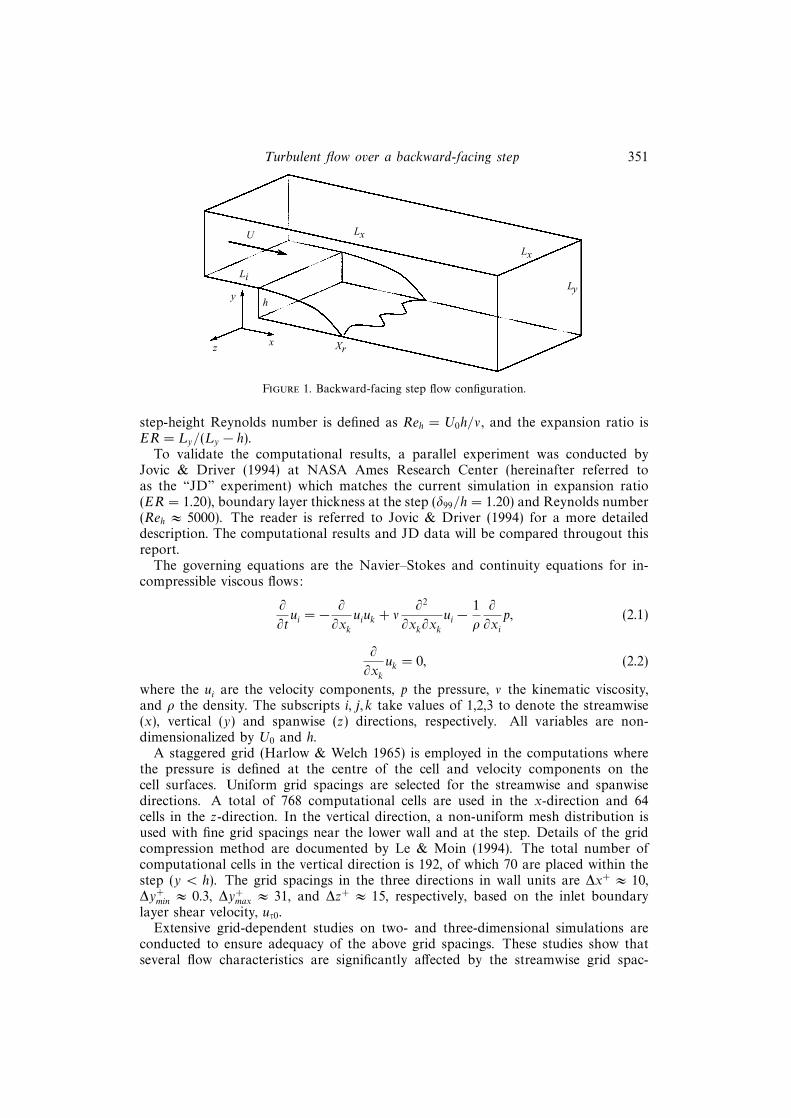
Figure 1 shows the schematic view of the flow domain used in the three-dimensionalsimulation. The computational domain consists of a streamwise length Lx = 30h,including an inlet section Li = 10h prior to the sudden expansion, vertical heightLy = 6h and spanwise width Lz = 4h, where h is the step height. The coordinatesystem is placed at the lower step corner as shown in figure 1. The mean inflow velocityprofile, U(y), imposed at the left boundary x = −Li is a flat-plate turbulent boundarylayer profile (Spalart 1988), with U0 being the maximum mean inlet velocity. The
Turbulent flow over a backward-facing step 351
y
z x
U
Li
Lx
Lx
Ly
Xr
h
Figure 1. Backward-facing step flow configuration.
step-height Reynolds number is defined as Reh = U0h/ν, and the expansion ratio isER = Ly/(Ly − h).
To validate the computational results, a parallel experiment was conducted byJovic & Driver (1994) at NASA Ames Research Center (hereinafter referred toas the “JD” experiment) which matches the current simulation in expansion ratio(ER = 1.20), boundary layer thickness at the step (δ99/h = 1.20) and Reynolds number(Reh ≈ 5000). The reader is referred to Jovic & Driver (1994) for a more detaileddescription. The computational results and JD data will be compared througout thisreport.
The governing equations are the Navier–Stokes and continuity equations for in-compressible viscous flows:
∂
∂tui = − ∂
∂xkuiuk + ν
∂2
∂xk∂xkui −
1
ρ
∂
∂xip, (2.1)
∂
∂xkuk = 0, (2.2)
where the ui are the velocity components, p the pressure, ν the kinematic viscosity,and ρ the density. The subscripts i, j, k take values of 1,2,3 to denote the streamwise(x), vertical (y) and spanwise (z) directions, respectively. All variables are non-dimensionalized by U0 and h.
A staggered grid (Harlow & Welch 1965) is employed in the computations wherethe pressure is defined at the centre of the cell and velocity components on thecell surfaces. Uniform grid spacings are selected for the streamwise and spanwisedirections. A total of 768 computational cells are used in the x-direction and 64cells in the z-direction. In the vertical direction, a non-uniform mesh distribution isused with fine grid spacings near the lower wall and at the step. Details of the gridcompression method are documented by Le & Moin (1994). The total number ofcomputational cells in the vertical direction is 192, of which 70 are placed within thestep (y < h). The grid spacings in the three directions in wall units are ∆x+ ≈ 10,∆y+
min ≈ 0.3, ∆y+max ≈ 31, and ∆z+ ≈ 15, respectively, based on the inlet boundary
layer shear velocity, uτ0.Extensive grid-dependent studies on two- and three-dimensional simulations are
conducted to ensure adequacy of the above grid spacings. These studies show thatseveral flow characteristics are significantly affected by the streamwise grid spac-
352 H. Le, P. Moin and J. Kim
ings. (a) Insufficient spatial resolution causes an otherwise steady flow to becomequasi-periodic (Le & Moin 1994). Recent work by Gresho et al. (1993) has alsoindependently shown that insufficient resolution will result in an unsteady numericalsolutions in backward-facing step simulations. (b) For the Reynolds number consid-ered in this study, a minimum of 512 streamwise cells in the post-expansion region(∆x+ ≈ 10 based on uτ0) is required to adequately resolve the unsteady flow structures.A 10% reduction in the reattachment length is also observed as the number of cellsis increased from 320 to 512. Further streamwise grid refinement does not resultin significant improvements. (c) Vertical grid refinement is necessary at the step forthe correct development of the near-wall turbulence in the entry section. The post-expansion flow characteristics are affected only by the vertical grid spacings at thebottom wall. The grid size at the step and bottom wall of ∆y+
min ≈ 0.3 (based on uτ0)is adequate for this purpose. (d) The spanwise resolution of 64 cells (∆z+ ≈ 15 basedon uτ0) appears to be sufficient for the Reynolds number considered. Doubling thespanwise grid cells does not improve the first-order statistics. However, examinationof one-dimesional energy spectra indicates that higher spanwise resolution is desirableto resolve the small-scale structures at y+ < 10.
2.2. Boundary conditions
A no-stress wall is applied at the upper boundary of the computational domain. Thevelocities at the no-stress wall are
v = 0,∂u
∂y=∂w
∂y= 0. (2.3)
In the spanwise direction, the flow is assumed to be statistically homogeneous andperiodic boundary conditions are used. No-slip boundary conditions are used at allother walls.
The mean inlet velocity profile, U(y), is obtained from Spalart’s (1988) boundarylayer simulation at Reθ = 670, where θ is the momentum thickness. The boundarylayer thickness is δ99 = 1.2h. The corresponding step-height Reynolds number isReh ≈ 5100. The time-dependent velocities prescribed at the inlet consist of U(y)and the imposed fluctuations, u′i(y, z, t). Lee, Lele & Moin (1992) described a methodof generating inflow fluctuations with a prescribed energy spectrum. However, theirmethod is not readily applicable to the generation of inlet turbulence for the backward-facing step flow because of the inhomogeneity in the y-direction. The same basicmethod is thus applied in this study, but the resulting u′i are scaled such that the
calculated fluctuations conform to all four Reynolds stress components, u′2, v′2, w′2
and u′v′, associated with the inlet boundary layer profile from Spalart (1988). Detailsof the method are described in Le & Moin (1994). The use of Lee et al.’s (1992)procedure ensures that the resulting signals do not contain excessive small-scalemotions which would have resulted if simply random numbers were used to generateu′, v′ and w′.
Although this procedure gives a set of stochastic signals that satisfy a prescribedset of second-order statistics, the flow quickly loses its statistical characteristics withinthe first few step heights from the inlet (Le & Moin 1994), and slowly recovers aftera transition length. This initial transition is due to the unphysical (structureless) inletturbulence which was a result of the randomized phase angles in the Lee et al.’s (1992)method. A transition length of about 10h is required for the recovery of turbulentcharacteristics. In our calculations the mean flow reaches to within 6% of the targetvalues of Spalart (1988) after approximately 7 step heights.
Turbulent flow over a backward-facing step 353
The exit boundary condition is the convective condition used by Lowery & Reynolds(1986) in numerical simulations of spatially evolving mixing layers. Pauley, Moin& Reynolds (1988) showed that, for unsteady problems, the convective boundarycondition is suitable for moving vortical structures out of the computational domain.The time-dependent condition of any velocity component ui at the exit plane (x = Lx)is taken as
∂ui∂t
+Uc
∂ui∂x
= 0. (2.4)
Uc is the convection velocity which is the constant mean exit velocity. Examinationof several statistical quantities from three-dimensional simulations indicates that themost severe effects of the outflow boundary conditions on the flow statistics areconfined to within one step height from the exit (Le & Moin 1994).
2.3. Time advancement
The governing equations are time-advanced using a semi-implicit method. Theadvancement scheme for the velocity components ui is a compact-storage third-orderRunge–Kutta scheme (Spalart 1987 and Spalart, Moser & Rogers 1991) which hasan explicit treatment for the convective terms and implicit for the viscous term. Thethree-substep Runge–Kutta scheme is combined with the fractional step procedure(Kim & Moin 1985): the method of Le & Moin (1991) is used which allowed forthe advancement of the velocity field through the substeps without satisfying thecontinuity equation at each Runge–Kutta substep. The velocities are projected ontothe divergence-free field only at the last substep. The convective terms are modifiedto preserve the second-order accuracy of the scheme.
The Poisson equation for pressure is solved using a two-iteration capacitance matrixmethod developed by Schumann & Benner (1982). The reader is referred to Le &Moin (1994) for the detailed development of the capacitance matrix method which istailored to the specific configuration and boundary conditions of the backward-facingstep.
The time step in the current simulation is fixed at ∆t = 0.0018h/U0 which keepsthe CFL number below 1.15. The algorithm requires approximately 13 mega-wordsof memory. Each time step uses 22 CPU seconds on the CRAY C-90, about 10seconds of which is devoted to solving the Poisson equation. The efficiency rating ofthe program is approximately 450 mega-flops.
The total simulation time is ttotal = 382h/U0. Approximately 11 ‘flow-through’ times(or ≈ 273h/U0) of the total simulation time is discarded to allow for the passageof initial transients. The ‘flow-through’ time here is defined as the convection timethrough the post-expansion section of 20h at the mean convective speed, Uc ≈ 0.8U0.The necessity of using a large initial transient period is due to the large residencetime of fluid particles in the recirculation zone. The statistical data set, including theReynolds stress budgets, is accumulated over the remaining time, ∆Tave = 109h/U0
or 6070 samples (one sample at every 10 time steps).
3. Results and discussion3.1. Unsteady flow characteristics
Friedrich & Arnal (1990) observed from their LES results that the free-shear layeremanating from the step had a vertical motion causing the reattachment location tooscillate. A low-frequency ‘flapping’ motion of the flow was also reported by Eaton &
354 H. Le, P. Moin and J. Kim
0 5 10 15
x /h
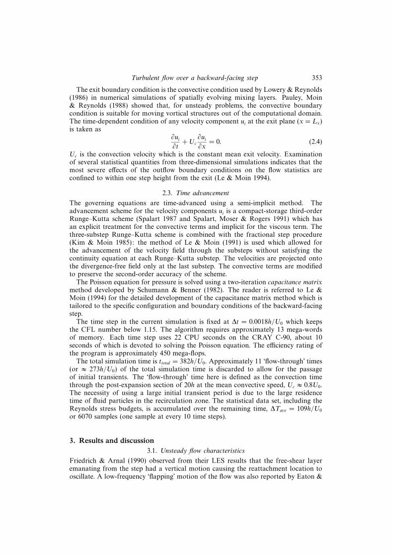
Figure 2. Instantanous spanwise vorticity (ωz) contours: , −1.0U0/h contours;, 1.0U0/h contours.
380360340320300280
tU0/h
5
6
7
8
Xr
h
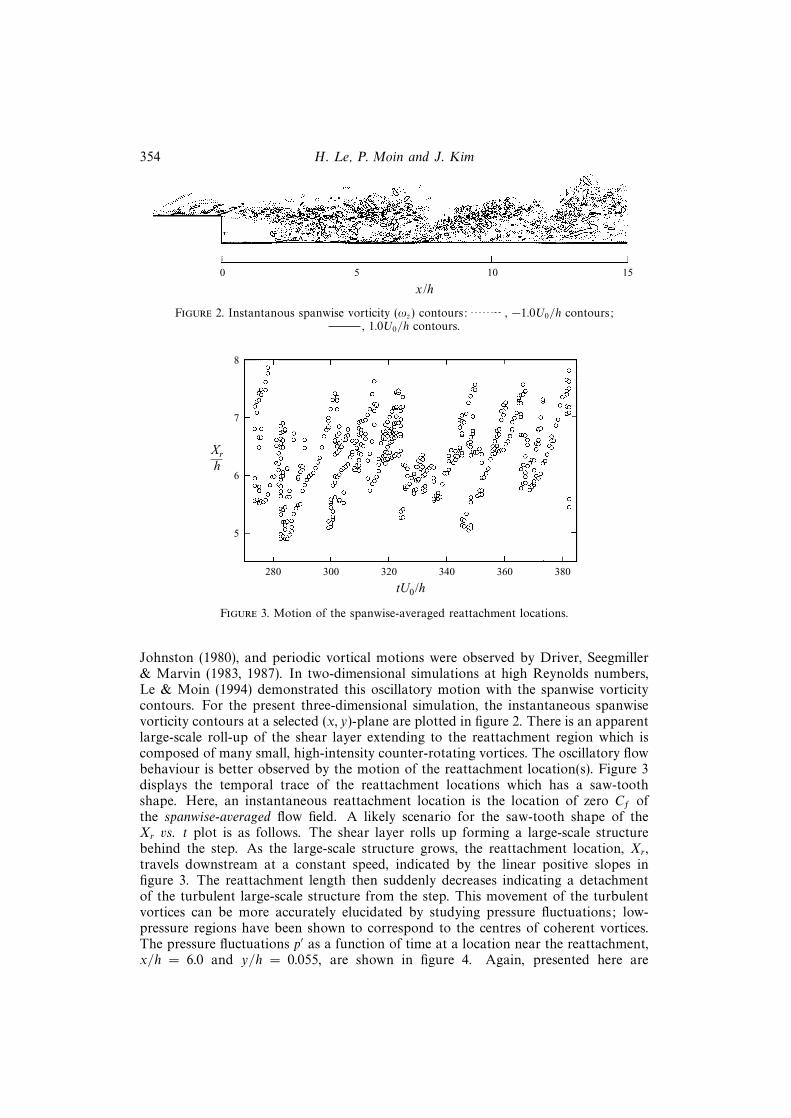
Figure 3. Motion of the spanwise-averaged reattachment locations.
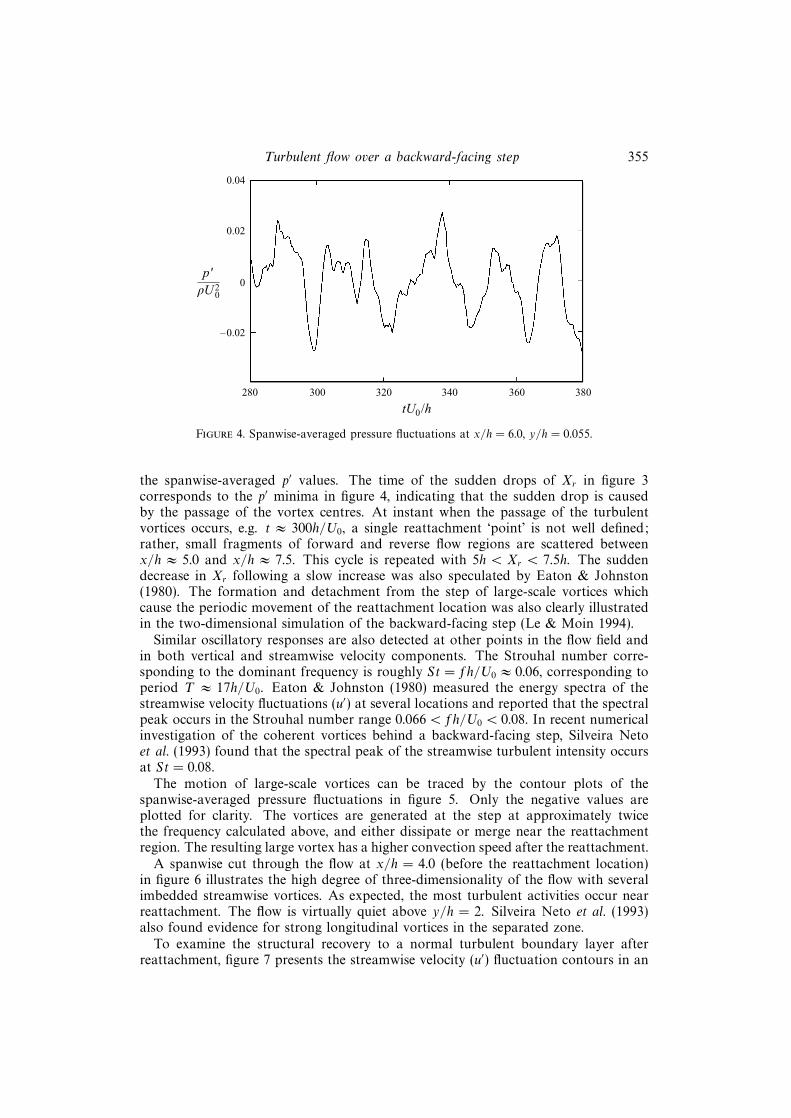
Johnston (1980), and periodic vortical motions were observed by Driver, Seegmiller& Marvin (1983, 1987). In two-dimensional simulations at high Reynolds numbers,Le & Moin (1994) demonstrated this oscillatory motion with the spanwise vorticitycontours. For the present three-dimensional simulation, the instantaneous spanwisevorticity contours at a selected (x, y)-plane are plotted in figure 2. There is an apparentlarge-scale roll-up of the shear layer extending to the reattachment region which iscomposed of many small, high-intensity counter-rotating vortices. The oscillatory flowbehaviour is better observed by the motion of the reattachment location(s). Figure 3displays the temporal trace of the reattachment locations which has a saw-toothshape. Here, an instantaneous reattachment location is the location of zero Cf ofthe spanwise-averaged flow field. A likely scenario for the saw-tooth shape of theXr vs. t plot is as follows. The shear layer rolls up forming a large-scale structurebehind the step. As the large-scale structure grows, the reattachment location, Xr ,travels downstream at a constant speed, indicated by the linear positive slopes infigure 3. The reattachment length then suddenly decreases indicating a detachmentof the turbulent large-scale structure from the step. This movement of the turbulentvortices can be more accurately elucidated by studying pressure fluctuations; low-pressure regions have been shown to correspond to the centres of coherent vortices.The pressure fluctuations p′ as a function of time at a location near the reattachment,x/h = 6.0 and y/h = 0.055, are shown in figure 4. Again, presented here are
Turbulent flow over a backward-facing step 355
380360340320300280
tU0/h
–0.02
0p ′
qU20
0.02
0.04
Figure 4. Spanwise-averaged pressure fluctuations at x/h = 6.0, y/h = 0.055.
the spanwise-averaged p′ values. The time of the sudden drops of Xr in figure 3corresponds to the p′ minima in figure 4, indicating that the sudden drop is causedby the passage of the vortex centres. At instant when the passage of the turbulentvortices occurs, e.g. t ≈ 300h/U0, a single reattachment ‘point’ is not well defined;rather, small fragments of forward and reverse flow regions are scattered betweenx/h ≈ 5.0 and x/h ≈ 7.5. This cycle is repeated with 5h < Xr < 7.5h. The suddendecrease in Xr following a slow increase was also speculated by Eaton & Johnston(1980). The formation and detachment from the step of large-scale vortices whichcause the periodic movement of the reattachment location was also clearly illustratedin the two-dimensional simulation of the backward-facing step (Le & Moin 1994).
Similar oscillatory responses are also detected at other points in the flow field andin both vertical and streamwise velocity components. The Strouhal number corre-sponding to the dominant frequency is roughly St = fh/U0 ≈ 0.06, corresponding toperiod T ≈ 17h/U0. Eaton & Johnston (1980) measured the energy spectra of thestreamwise velocity fluctuations (u′) at several locations and reported that the spectralpeak occurs in the Strouhal number range 0.066 < fh/U0 < 0.08. In recent numericalinvestigation of the coherent vortices behind a backward-facing step, Silveira Netoet al. (1993) found that the spectral peak of the streamwise turbulent intensity occursat St = 0.08.
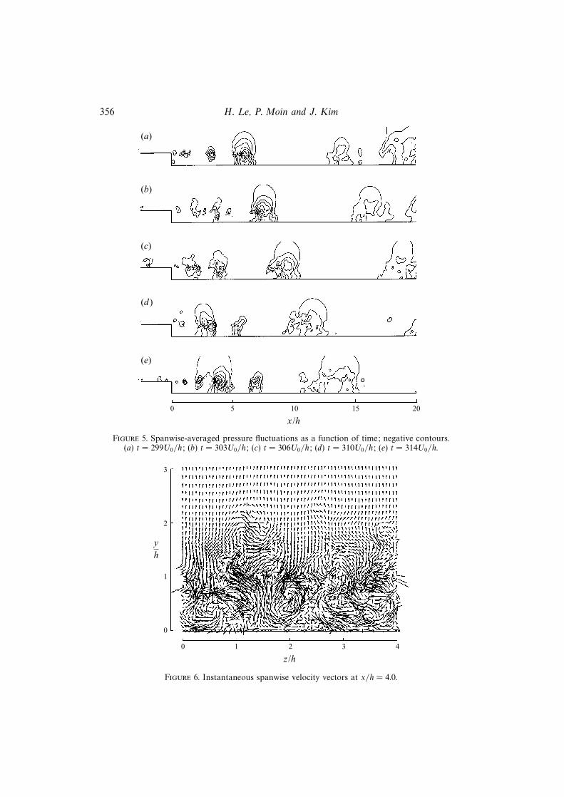
The motion of large-scale vortices can be traced by the contour plots of thespanwise-averaged pressure fluctuations in figure 5. Only the negative values areplotted for clarity. The vortices are generated at the step at approximately twicethe frequency calculated above, and either dissipate or merge near the reattachmentregion. The resulting large vortex has a higher convection speed after the reattachment.
A spanwise cut through the flow at x/h = 4.0 (before the reattachment location)in figure 6 illustrates the high degree of three-dimensionality of the flow with severalimbedded streamwise vortices. As expected, the most turbulent activities occur nearreattachment. The flow is virtually quiet above y/h = 2. Silveira Neto et al. (1993)also found evidence for strong longitudinal vortices in the separated zone.
To examine the structural recovery to a normal turbulent boundary layer afterreattachment, figure 7 presents the streamwise velocity (u′) fluctuation contours in an
356 H. Le, P. Moin and J. Kim
(a)
(b)
(c)
(d )
(e)
0 5 10 15 20
x /h
Figure 5. Spanwise-averaged pressure fluctuations as a function of time; negative contours.(a) t = 299U0/h; (b) t = 303U0/h; (c) t = 306U0/h; (d) t = 310U0/h; (e) t = 314U0/h.
3
2
1
0
yh
0 1 2 3 4
z /h
Figure 6. Instantaneous spanwise velocity vectors at x/h = 4.0.
Turbulent flow over a backward-facing step 357
0 5 10 15 20
x /h
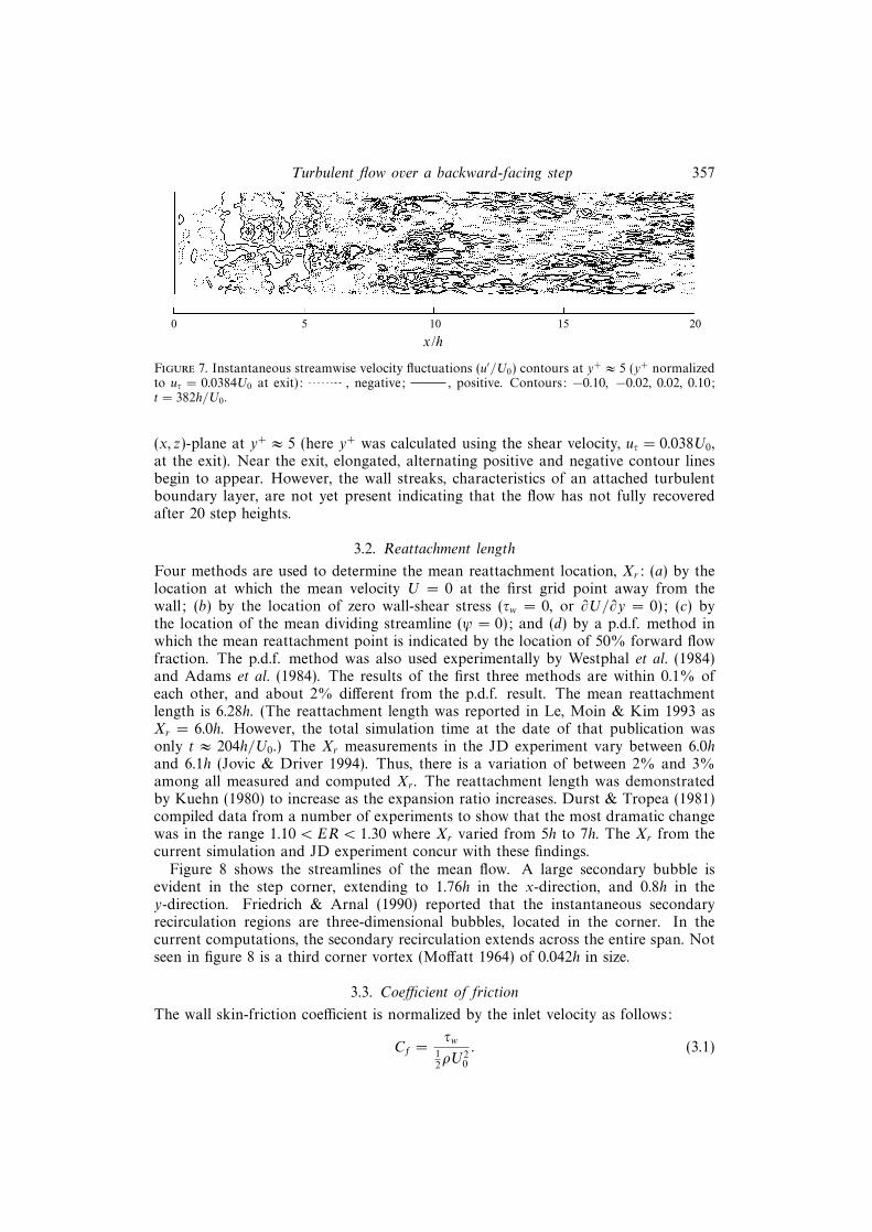
Figure 7. Instantaneous streamwise velocity fluctuations (u′/U0) contours at y+ ≈ 5 (y+ normalizedto uτ = 0.0384U0 at exit): , negative; , positive. Contours: −0.10, −0.02, 0.02, 0.10;t = 382h/U0.
(x, z)-plane at y+ ≈ 5 (here y+ was calculated using the shear velocity, uτ = 0.038U0,at the exit). Near the exit, elongated, alternating positive and negative contour linesbegin to appear. However, the wall streaks, characteristics of an attached turbulentboundary layer, are not yet present indicating that the flow has not fully recoveredafter 20 step heights.
3.2. Reattachment length
Four methods are used to determine the mean reattachment location, Xr: (a) by thelocation at which the mean velocity U = 0 at the first grid point away from thewall; (b) by the location of zero wall-shear stress (τw = 0, or ∂U/∂y = 0); (c) bythe location of the mean dividing streamline (ψ = 0); and (d) by a p.d.f. method inwhich the mean reattachment point is indicated by the location of 50% forward flowfraction. The p.d.f. method was also used experimentally by Westphal et al. (1984)and Adams et al. (1984). The results of the first three methods are within 0.1% ofeach other, and about 2% different from the p.d.f. result. The mean reattachmentlength is 6.28h. (The reattachment length was reported in Le, Moin & Kim 1993 asXr = 6.0h. However, the total simulation time at the date of that publication wasonly t ≈ 204h/U0.) The Xr measurements in the JD experiment vary between 6.0hand 6.1h (Jovic & Driver 1994). Thus, there is a variation of between 2% and 3%among all measured and computed Xr . The reattachment length was demonstratedby Kuehn (1980) to increase as the expansion ratio increases. Durst & Tropea (1981)compiled data from a number of experiments to show that the most dramatic changewas in the range 1.10 < ER < 1.30 where Xr varied from 5h to 7h. The Xr from thecurrent simulation and JD experiment concur with these findings.
Figure 8 shows the streamlines of the mean flow. A large secondary bubble isevident in the step corner, extending to 1.76h in the x-direction, and 0.8h in they-direction. Friedrich & Arnal (1990) reported that the instantaneous secondaryrecirculation regions are three-dimensional bubbles, located in the corner. In thecurrent computations, the secondary recirculation extends across the entire span. Notseen in figure 8 is a third corner vortex (Moffatt 1964) of 0.042h in size.
3.3. Coefficient of friction
The wall skin-friction coefficient is normalized by the inlet velocity as follows:
Cf =τw
12ρU2
0
. (3.1)
358 H. Le, P. Moin and J. Kim
0 5 10 15 20
x /h
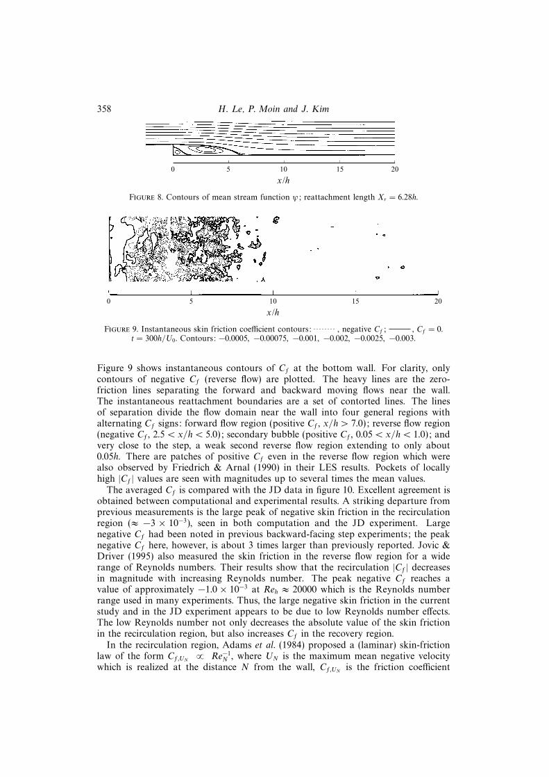
Figure 8. Contours of mean stream function ψ; reattachment length Xr = 6.28h.
0 5 10 15 20
x /h
Figure 9. Instantaneous skin friction coefficient contours: , negative Cf; , Cf = 0.t = 300h/U0. Contours: −0.0005, −0.00075, −0.001, −0.002, −0.0025, −0.003.
Figure 9 shows instantaneous contours of Cf at the bottom wall. For clarity, onlycontours of negative Cf (reverse flow) are plotted. The heavy lines are the zero-friction lines separating the forward and backward moving flows near the wall.The instantaneous reattachment boundaries are a set of contorted lines. The linesof separation divide the flow domain near the wall into four general regions withalternating Cf signs: forward flow region (positive Cf , x/h > 7.0); reverse flow region(negative Cf , 2.5 < x/h < 5.0); secondary bubble (positive Cf , 0.05 < x/h < 1.0); andvery close to the step, a weak second reverse flow region extending to only about0.05h. There are patches of positive Cf even in the reverse flow region which werealso observed by Friedrich & Arnal (1990) in their LES results. Pockets of locallyhigh |Cf | values are seen with magnitudes up to several times the mean values.
The averaged Cf is compared with the JD data in figure 10. Excellent agreement isobtained between computational and experimental results. A striking departure fromprevious measurements is the large peak of negative skin friction in the recirculationregion (≈ −3 × 10⁻³), seen in both computation and the JD experiment. Largenegative Cf had been noted in previous backward-facing step experiments; the peaknegative Cf here, however, is about 3 times larger than previously reported. Jovic &Driver (1995) also measured the skin friction in the reverse flow region for a widerange of Reynolds numbers. Their results show that the recirculation |Cf | decreasesin magnitude with increasing Reynolds number. The peak negative Cf reaches avalue of approximately −1.0 × 10⁻³ at Reh ≈ 20000 which is the Reynolds numberrange used in many experiments. Thus, the large negative skin friction in the currentstudy and in the JD experiment appears to be due to low Reynolds number effects.The low Reynolds number not only decreases the absolute value of the skin frictionin the recirculation region, but also increases Cf in the recovery region.
In the recirculation region, Adams et al. (1984) proposed a (laminar) skin-frictionlaw of the form Cf,UN
∝ Re−1N , where UN is the maximum mean negative velocity
which is realized at the distance N from the wall, Cf,UNis the friction coefficient
Turbulent flow over a backward-facing step 359
0 5 10 15 20
x /h
0.004
0.002
0
–0.002
–0.004
Cf
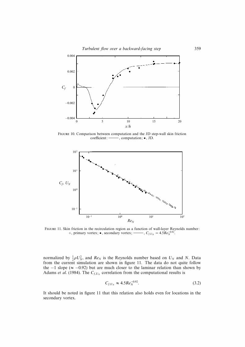
Figure 10. Comparison between computation and the JD step-wall skin frictioncoefficient: , computation; • , JD.
102
101
100
10–1
10–1 100 101 102
ReN
Cf , UN
Figure 11. Skin friction in the recirculation region as a function of wall-layer Reynolds number:◦ , primary vortex; • , secondary vortex; , Cf,UN = 4.5Re−0.92
N .
normalized by 12ρU2
N , and ReN is the Reynolds number based on UN and N. Datafrom the current simulation are shown in figure 11. The data do not quite followthe −1 slope (≈ −0.92) but are much closer to the laminar relation than shown byAdams et al. (1984). The Cf,UN
correlation from the computational results is
Cf,UN≈ 4.5Re−0.92
N . (3.2)
It should be noted in figure 11 that this relation also holds even for locations in thesecondary vortex.
360 H. Le, P. Moin and J. Kim
0.2
0 5 10 15
x/h
Cp0.1
0
20
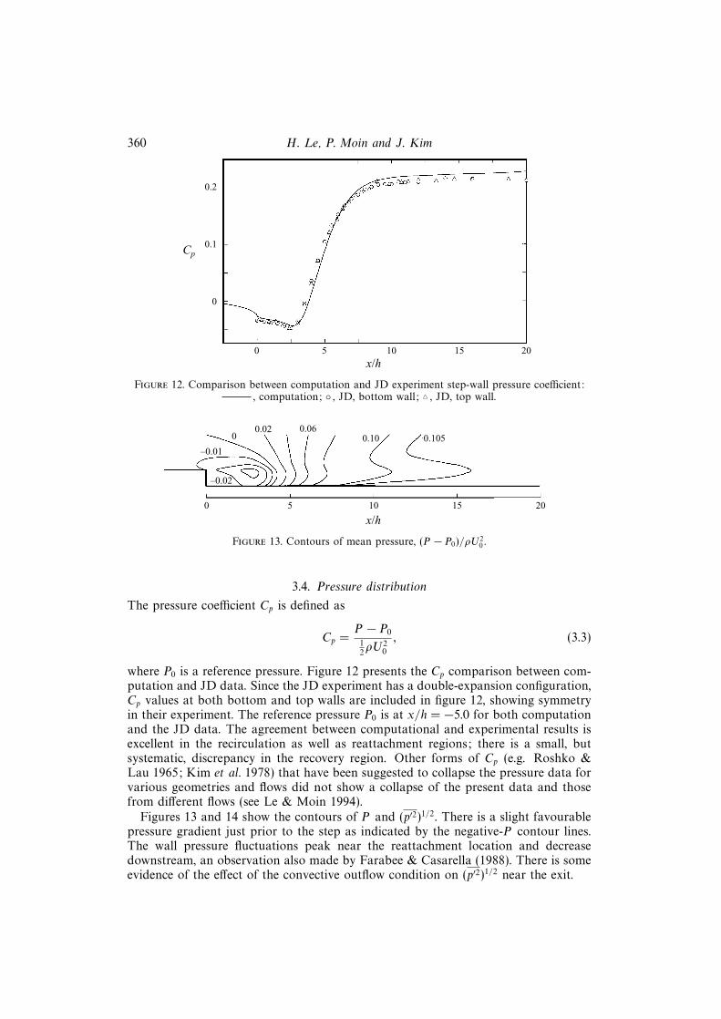
Figure 12. Comparison between computation and JD experiment step-wall pressure coefficient:, computation; ◦ , JD, bottom wall; 4 , JD, top wall.
0 5 10 15 20
x/h
–0.02
–0.01
00.02 0.06
0.10 0.105
Figure 13. Contours of mean pressure, (P − P0)/ρU20 .
3.4. Pressure distribution
The pressure coefficient Cp is defined as
Cp =P − P0
12ρU2
0
, (3.3)
where P0 is a reference pressure. Figure 12 presents the Cp comparison between com-putation and JD data. Since the JD experiment has a double-expansion configuration,Cp values at both bottom and top walls are included in figure 12, showing symmetryin their experiment. The reference pressure P0 is at x/h = −5.0 for both computationand the JD data. The agreement between computational and experimental results isexcellent in the recirculation as well as reattachment regions; there is a small, butsystematic, discrepancy in the recovery region. Other forms of Cp (e.g. Roshko &Lau 1965; Kim et al. 1978) that have been suggested to collapse the pressure data forvarious geometries and flows did not show a collapse of the present data and thosefrom different flows (see Le & Moin 1994).
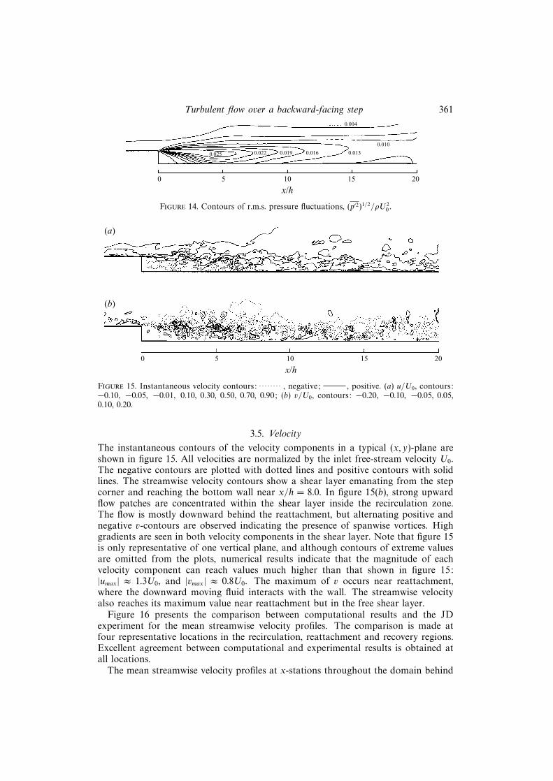
Figures 13 and 14 show the contours of P and (p′2)1/2. There is a slight favourablepressure gradient just prior to the step as indicated by the negative-P contour lines.The wall pressure fluctuations peak near the reattachment location and decreasedownstream, an observation also made by Farabee & Casarella (1988). There is someevidence of the effect of the convective outflow condition on (p′2)1/2 near the exit.
Turbulent flow over a backward-facing step 361
0 5 10 15 20
x/h
0.025 0.022 0.019 0.016 0.013
0.010
0.004
Figure 14. Contours of r.m.s. pressure fluctuations, (p′2)1/2/ρU20 .
0 5 10 15 20
x/h
(a)
(b)
Figure 15. Instantaneous velocity contours: , negative; , positive. (a) u/U0, contours:−0.10, −0.05, −0.01, 0.10, 0.30, 0.50, 0.70, 0.90; (b) v/U0, contours: −0.20, −0.10, −0.05, 0.05,0.10, 0.20.
3.5. Velocity
The instantaneous contours of the velocity components in a typical (x, y)-plane areshown in figure 15. All velocities are normalized by the inlet free-stream velocity U0.The negative contours are plotted with dotted lines and positive contours with solidlines. The streamwise velocity contours show a shear layer emanating from the stepcorner and reaching the bottom wall near x/h = 8.0. In figure 15(b), strong upwardflow patches are concentrated within the shear layer inside the recirculation zone.The flow is mostly downward behind the reattachment, but alternating positive andnegative v-contours are observed indicating the presence of spanwise vortices. Highgradients are seen in both velocity components in the shear layer. Note that figure 15is only representative of one vertical plane, and although contours of extreme valuesare omitted from the plots, numerical results indicate that the magnitude of eachvelocity component can reach values much higher than that shown in figure 15:|umax| ≈ 1.3U0, and |vmax| ≈ 0.8U0. The maximum of v occurs near reattachment,where the downward moving fluid interacts with the wall. The streamwise velocityalso reaches its maximum value near reattachment but in the free shear layer.
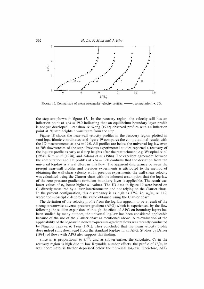
Figure 16 presents the comparison between computational results and the JDexperiment for the mean streamwise velocity profiles. The comparison is made atfour representative locations in the recirculation, reattachment and recovery regions.Excellent agreement between computational and experimental results is obtained atall locations.
The mean streamwise velocity profiles at x-stations throughout the domain behind
362 H. Le, P. Moin and J. Kim
0
3
2
1
yh
0 0 0 0.50 1.0
U /U0
x /h = 4 6 10 19
Figure 16. Comparison of mean streamwise velocity profiles: , computation; • , JD.
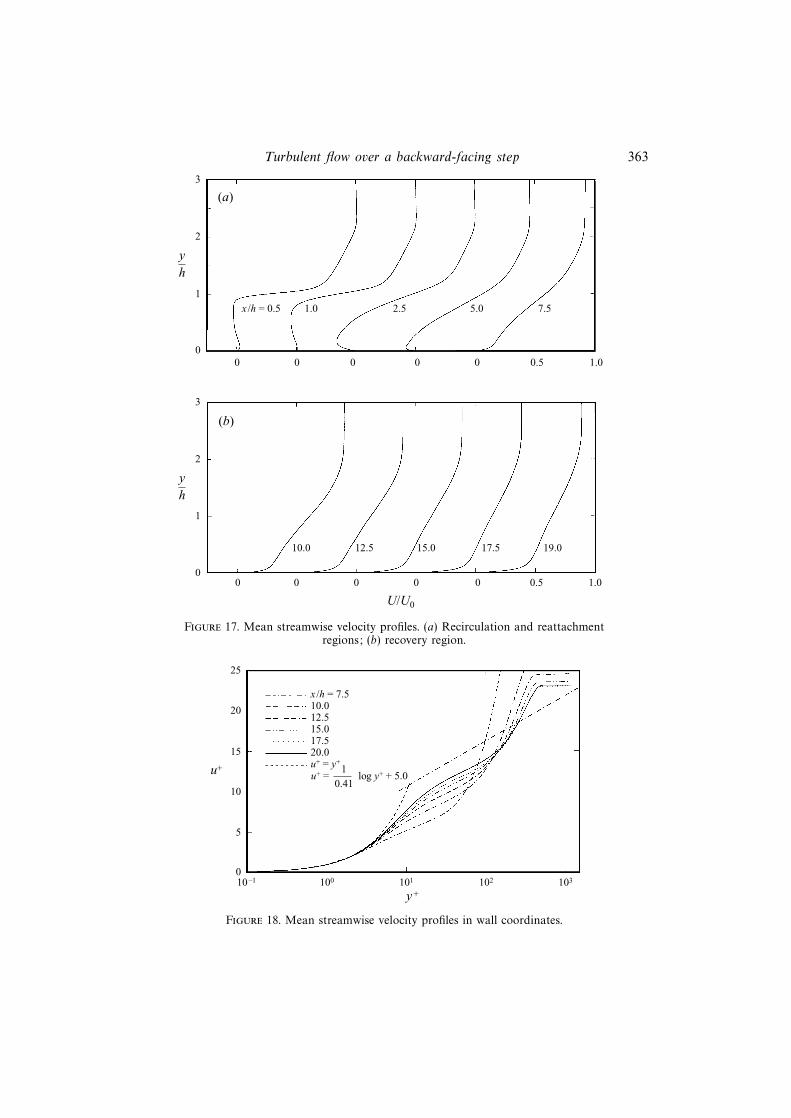
the step are shown in figure 17. In the recovery region, the velocity still has aninflection point at x/h = 19.0 indicating that an equilibrium boundary layer profileis not yet developed. Bradshaw & Wong (1972) observed profiles with an inflectionpoint at 50 step heights downstream from the step.
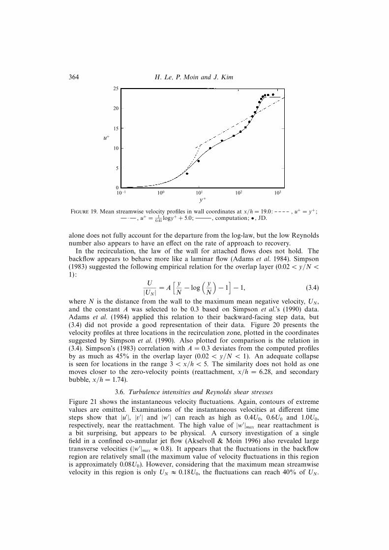
Figure 18 shows the near-wall velocity profiles in the recovery region plotted insemi-logarithmic coordinates, and figure 19 compares the computational results withthe JD measurements at x/h = 19.0. All profiles are below the universal log-law evenat 20h downstream of the step. Previous experimental studies reported a recovery ofthe log-law profile as early as 6 step heights after the reattachment, e.g. Westphal et al.(1984), Kim et al. (1978), and Adams et al. (1984). The excellent agreement betweenthe computation and JD profiles at x/h = 19.0 confirms that the deviation from theuniversal log-law is a real effect in this flow. The apparent discrepancy between thepresent near-wall profiles and previous experiments is attributed to the method ofobtaining the wall-shear velocity uτ. In previous experiments, the wall-shear velocitywas calculated using the Clauser chart with the inherent assumption that the log-lawof the zero-pressure-gradient turbulent boundary layer is applicable. The result waslower values of uτ, hence higher u+ values. The JD data in figure 19 were based onCf directly measured by a laser interferometer, and not relying on the Clauser chart.In the present configuration, this discrepancy is as high as 17%, i.e. uτ/uτc ≈ 1.17,where the subscript c denotes the value obtained using the Clauser chart.
The deviation of the velocity profile from the log-law appears to be a result of thestrong streamwise adverse pressure gradient (APG) which is experienced by the flowfollowing the sudden expansion. Although the effect of APG on boundary layers hasbeen studied by many authors, the universal log-law has been considered applicablebecause of the use of the Clauser chart as mentioned above. A re-evaluation of theapplicability of the log-law in non-zero-pressure-gradient flows was recently conductedby Nagano, Tagawa & Tsuji (1991). They concluded that the mean velocity profiledoes indeed shift downward from the standard log-law in an APG. Studies by Driver(1991) of flows with APG also support this finding.
Since uτ is proportional to C1/2f , and as shown earlier, the calculated Cf in the
recovery region is high due to low Reynolds number effects, the profile of U/uτ inwall coordinates is further depressed below the universal log-law. Therefore, APG
Turbulent flow over a backward-facing step 363
(a)
(b)
0 0 0 0 0 0.5 1.0
x /h = 0.5 1.0 2.5 7.55.0
0 0 0 0 0 0.5 1.0
12.5 15.0 19.017.510.0
U/U0
3
2
1
0
yh
3
2
1
0
yh
Figure 17. Mean streamwise velocity profiles. (a) Recirculation and reattachmentregions; (b) recovery region.
25
20
15
10
5
0
x /h = 7.510.012.515.017.520.0u+ = y+
u+
10–1 100 101 102 103
y+
u+ = log y+ + 5.01
0.41
Figure 18. Mean streamwise velocity profiles in wall coordinates.
364 H. Le, P. Moin and J. Kim
25
20
15
10
5
0
u+
10–1 100 101 102 103
y+
Figure 19. Mean streamwise velocity profiles in wall coordinates at x/h = 19.0: , u+ = y+;, u+ = 1
0.41logy+ + 5.0; , computation; • , JD.
alone does not fully account for the departure from the log-law, but the low Reynoldsnumber also appears to have an effect on the rate of approach to recovery.
In the recirculation, the law of the wall for attached flows does not hold. Thebackflow appears to behave more like a laminar flow (Adams et al. 1984). Simpson(1983) suggested the following empirical relation for the overlap layer (0.02 < y/N <1):
U
|UN |= A
[ yN− log
( yN
)− 1]− 1, (3.4)
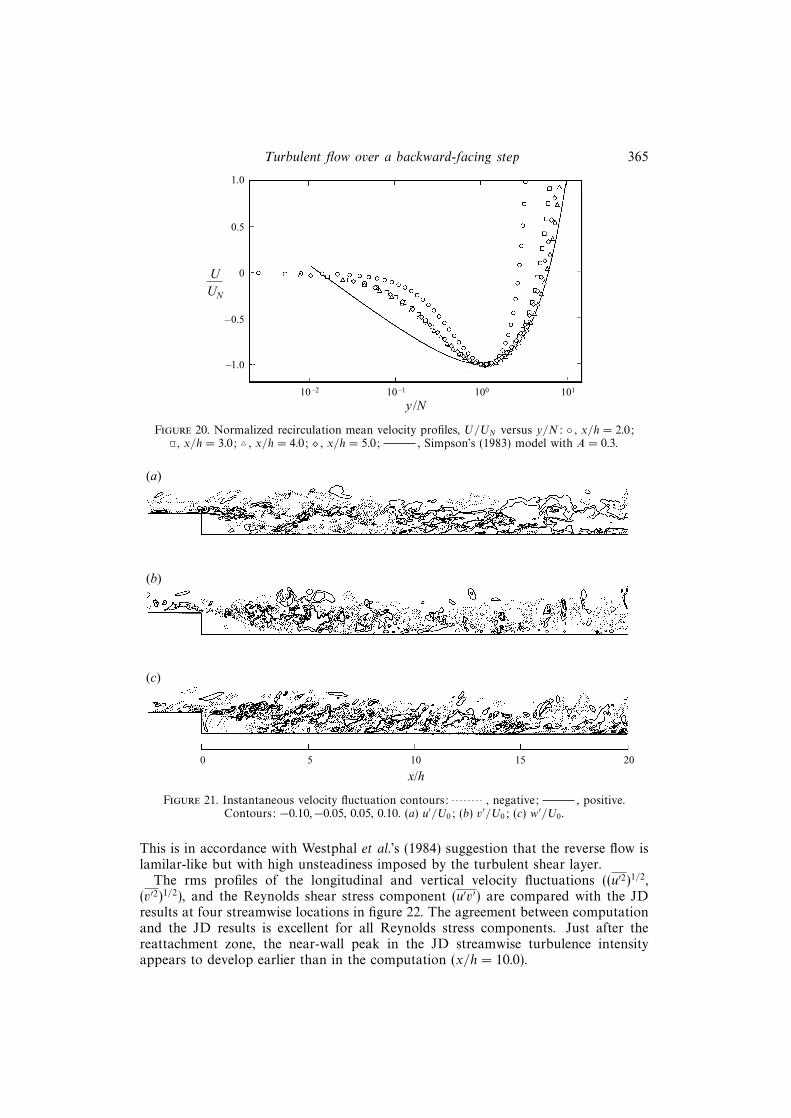
where N is the distance from the wall to the maximum mean negative velocity, UN ,and the constant A was selected to be 0.3 based on Simpson et al.’s (1990) data.Adams et al. (1984) applied this relation to their backward-facing step data, but(3.4) did not provide a good representation of their data. Figure 20 presents thevelocity profiles at three locations in the recirculation zone, plotted in the coordinatessuggested by Simpson et al. (1990). Also plotted for comparison is the relation in(3.4). Simpson’s (1983) correlation with A = 0.3 deviates from the computed profilesby as much as 45% in the overlap layer (0.02 < y/N < 1). An adequate collapseis seen for locations in the range 3 < x/h < 5. The similarity does not hold as onemoves closer to the zero-velocity points (reattachment, x/h = 6.28, and secondarybubble, x/h = 1.74).
3.6. Turbulence intensities and Reynolds shear stresses
Figure 21 shows the instantaneous velocity fluctuations. Again, contours of extremevalues are omitted. Examinations of the instantaneous velocities at different timesteps show that |u′|, |v′| and |w′| can reach as high as 0.4U0, 0.6U0 and 1.0U0,respectively, near the reattachment. The high value of |w′|max near reattachment isa bit surprising, but appears to be physical. A cursory investigation of a singlefield in a confined co-annular jet flow (Akselvoll & Moin 1996) also revealed largetransverse velocities (|w′|max ≈ 0.8). It appears that the fluctuations in the backflowregion are relatively small (the maximum value of velocity fluctuations in this regionis approximately 0.08U0). However, considering that the maximum mean streamwisevelocity in this region is only UN ≈ 0.18U0, the fluctuations can reach 40% of UN .
Turbulent flow over a backward-facing step 365
1.0
0.5
0
–0.5
–1.0
UUN
10–2 10–1 100 101
y /N
Figure 20. Normalized recirculation mean velocity profiles, U/UN versus y/N: ◦ , x/h = 2.0;, x/h = 3.0; 4 , x/h = 4.0; � , x/h = 5.0; , Simpson’s (1983) model with A = 0.3.
0 5 10 15 20
x/h
(a)
(b)
(c)
Figure 21. Instantaneous velocity fluctuation contours: , negative; , positive.Contours: −0.10,−0.05, 0.05, 0.10. (a) u′/U0; (b) v′/U0; (c) w′/U0.
This is in accordance with Westphal et al.’s (1984) suggestion that the reverse flow islamilar-like but with high unsteadiness imposed by the turbulent shear layer.
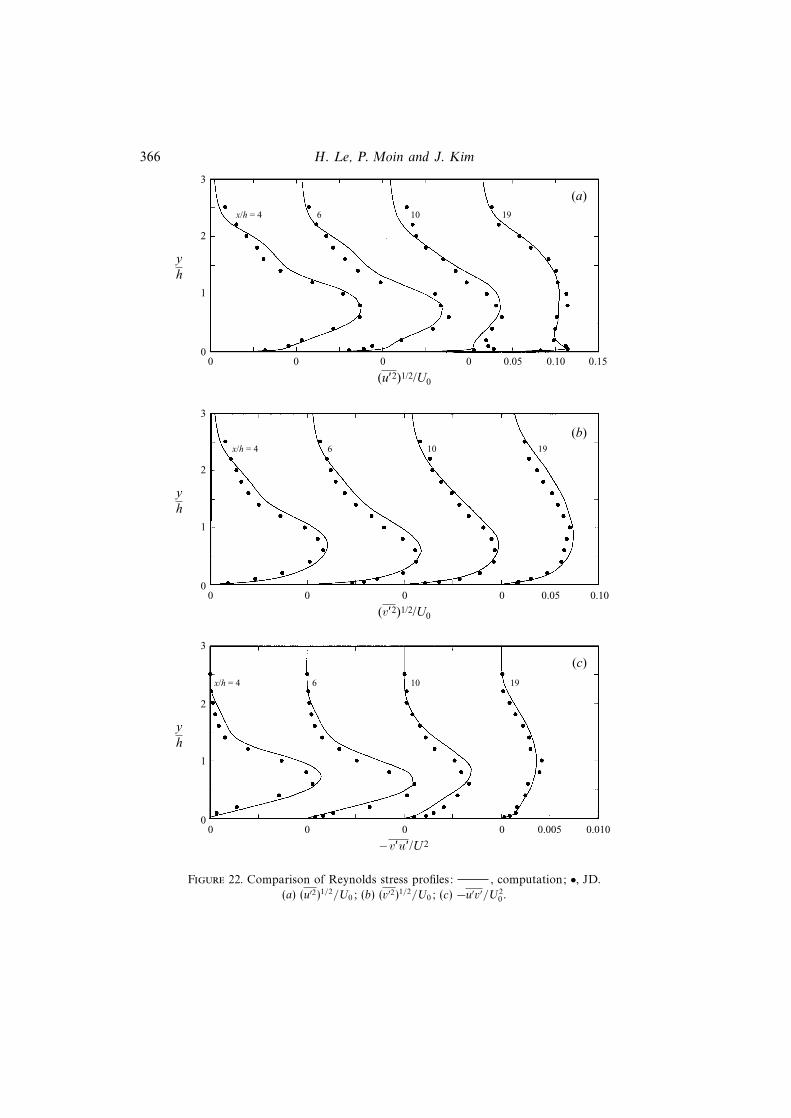
The rms profiles of the longitudinal and vertical velocity fluctuations ((u′2)1/2,(v′2)1/2), and the Reynolds shear stress component (u′v′) are compared with the JDresults at four streamwise locations in figure 22. The agreement between computationand the JD results is excellent for all Reynolds stress components. Just after thereattachment zone, the near-wall peak in the JD streamwise turbulence intensityappears to develop earlier than in the computation (x/h = 10.0).
366 H. Le, P. Moin and J. Kim
0 0 0.05 0.10 0.15
(u′2)1/2/U0
(a)
(b)
(c)
0 0
x/h = 4
0
1
2
3
yh
6 10 19
0 0 0.05 0.10
(v′2)1/2/U0
0 0
x/h = 4
0
1
2
3
yh
6 10 19
0 0 0.005 0.010
– v′u′/U2
0 0
x/h = 4
0
1
2
3
yh
6 10 19
Figure 22. Comparison of Reynolds stress profiles: , computation; •, JD.
(a) (u′2)1/2/U0; (b) (v′2)1/2/U0; (c) −u′v′/U20 .
Turbulent flow over a backward-facing step 367
q2/2
bud
get n
orm
aliz
ed b
y U
02 /h
(a)
0 0.05 0.10 0.15 0.2
0.010
0.005
0
–0.005
–0.010
(y – h)/h
q2/2
bud
get n
orm
aliz
ed b
y u
4 τ/ν
(b)
0 5 10 15 20
0.4
0.2
0
–0.2
y+
25
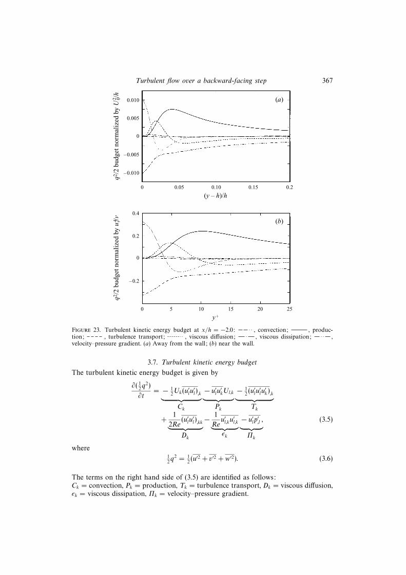
Figure 23. Turbulent kinetic energy budget at x/h = −2.0: , convection; , produc-tion; , turbulence transport; , viscous diffusion; , viscous dissipation; ,velocity–pressure gradient. (a) Away from the wall; (b) near the wall.
3.7. Turbulent kinetic energy budget
The turbulent kinetic energy budget is given by
∂( 12q2)
∂t= − 1
2Uk(u
′lu′l),k︸ ︷︷ ︸
Ck
− u′lu′kUl,k︸ ︷︷ ︸Pk
− 12(u′lu
′lu′k),k︸ ︷︷ ︸
Tk
+1
2Re(u′lu
′l),kk︸ ︷︷ ︸
Dk
− 1
Reu′l,ku
′l,k︸ ︷︷ ︸
εk
− u′lp′,l ,︸ ︷︷ ︸Πk
(3.5)
where12q2 = 1
2(u′2 + v′2 + w′2). (3.6)
The terms on the right hand side of (3.5) are identified as follows:Ck = convection, Pk = production, Tk = turbulence transport, Dk = viscous diffusion,εk = viscous dissipation, Πk = velocity–pressure gradient.
368 H. Le, P. Moin and J. Kim
q2/2
bud
get n
orm
aliz
ed b
y U
03/h
(a)
0 0.4 0.8 1.2 1.6
0.015
0.010
0
–0.005
–0.010
y/h
q2/2
bud
get n
orm
aliz
ed b
y u
4 τ/ν
(b)
0 5 10 15 20
1.5
1.0
0
–0.5
y+
25
0.005
–0.015
0.5
–1.0
–1.5
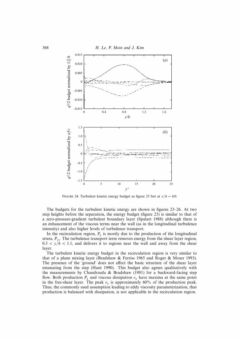
Figure 24. Turbulent kinetic energy budget as figure 23 but at x/h = 4.0.
The budgets for the turbulent kinetic energy are shown in figures 23–26. At twostep heights before the separation, the energy budget (figure 23) is similar to that ofa zero-pressure-gradient turbulent boundary layer (Spalart 1988) although there isan enhancement of the viscous terms near the wall (as in the longitudinal turbulenceintensity) and also higher levels of turbulence transport.
In the recirculation region, Pk is mostly due to the production of the longitudinalstress, P11. The turbulence transport term removes energy from the shear layer region,0.3 < y/h < 1.1, and delivers it to regions near the wall and away from the shearlayer.
The turbulent kinetic energy budget in the recirculation region is very similar tothat of a plane mixing layer (Bradshaw & Ferriss 1965 and Roger & Moser 1993).The presence of the ‘ground’ does not affect the basic structure of the shear layeremanating from the step (Hunt 1990). This budget also agrees qualitatively withthe measurements by Chandrsuda & Bradshaw (1981) for a backward-facing stepflow. Both production Pk and viscous dissipation εk have maxima at the same pointin the free-shear layer. The peak εk is approximately 60% of the production peak.Thus, the commonly used assumption leading to eddy viscosity parameterization, thatproduction is balanced with dissipation, is not applicable in the recirculation region.
Turbulent flow over a backward-facing step 369
q2/2
bud
get n
orm
aliz
ed b
y U
03/h
(a)
0 0.5 1.0 1.5 2.0
0.02
0.01
0
–0.01
y/h
q2/2
bud
get n
orm
aliz
ed b
y u
4 τ/ν
(b)
0 5 10 15 20
20
0
y+
25
10
–10
–20
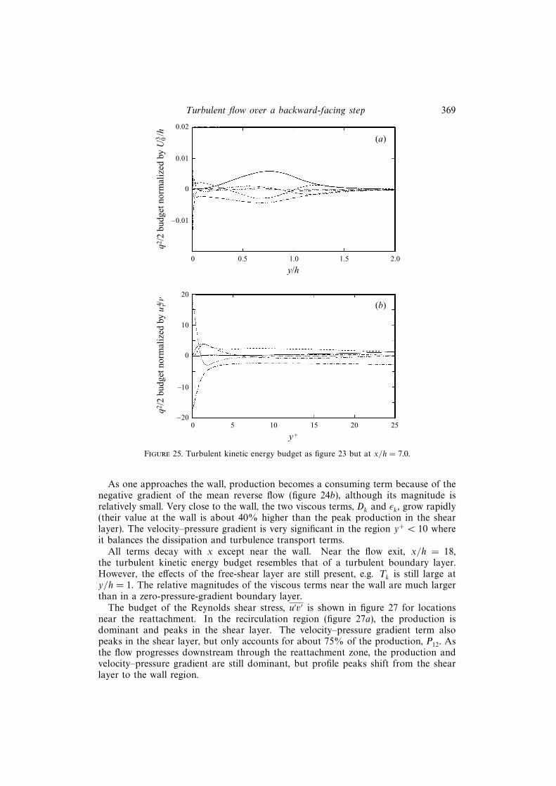
Figure 25. Turbulent kinetic energy budget as figure 23 but at x/h = 7.0.
As one approaches the wall, production becomes a consuming term because of thenegative gradient of the mean reverse flow (figure 24b), although its magnitude isrelatively small. Very close to the wall, the two viscous terms, Dk and εk , grow rapidly(their value at the wall is about 40% higher than the peak production in the shearlayer). The velocity–pressure gradient is very significant in the region y+ < 10 whereit balances the dissipation and turbulence transport terms.
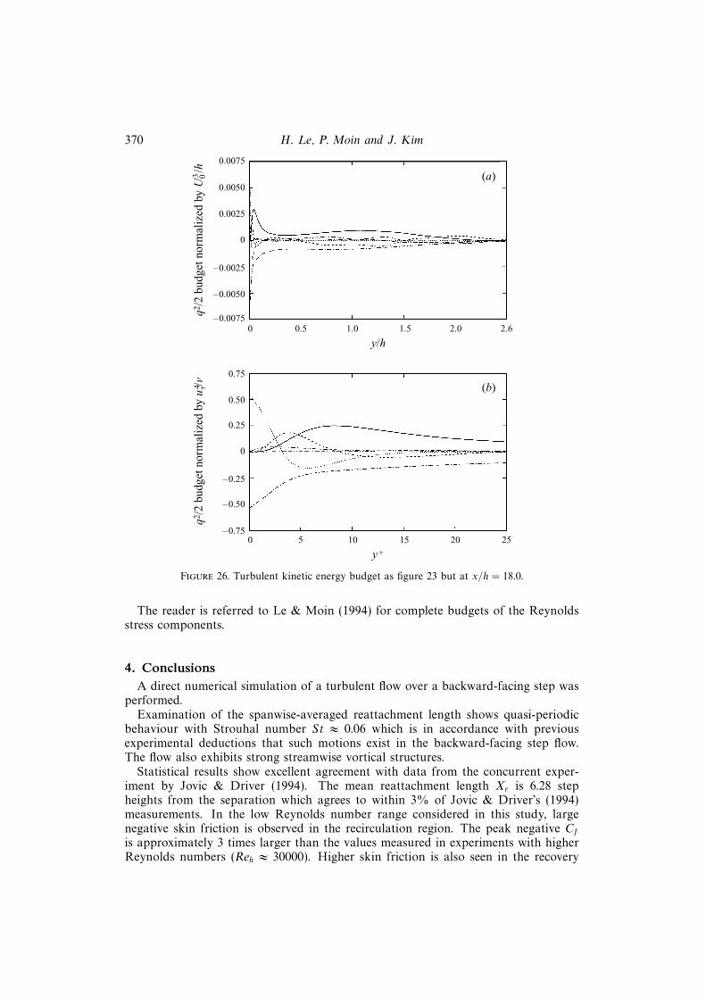
All terms decay with x except near the wall. Near the flow exit, x/h = 18,the turbulent kinetic energy budget resembles that of a turbulent boundary layer.However, the effects of the free-shear layer are still present, e.g. Tk is still large aty/h = 1. The relative magnitudes of the viscous terms near the wall are much largerthan in a zero-pressure-gradient boundary layer.
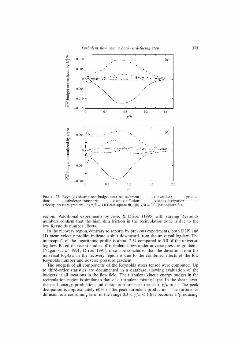
The budget of the Reynolds shear stress, u′v′ is shown in figure 27 for locationsnear the reattachment. In the recirculation region (figure 27a), the production isdominant and peaks in the shear layer. The velocity–pressure gradient term alsopeaks in the shear layer, but only accounts for about 75% of the production, P12. Asthe flow progresses downstream through the reattachment zone, the production andvelocity–pressure gradient are still dominant, but profile peaks shift from the shearlayer to the wall region.
370 H. Le, P. Moin and J. Kim
q2/2
bud
get n
orm
aliz
ed b
y U
03/h
(a)
0 0.5 1.0 1.5 2.0
0.0075
0.0050
0
–0.0025
y/h
q2/2
bud
get n
orm
aliz
ed b
y u
4 τ/ν
(b)
0 5 10 15 20
0.75
0
y+
25
0.50
–0.25
0.0025
–0.0050
–0.00752.6
0.25
–0.50
–0.75
Figure 26. Turbulent kinetic energy budget as figure 23 but at x/h = 18.0.
The reader is referred to Le & Moin (1994) for complete budgets of the Reynoldsstress components.
4. ConclusionsA direct numerical simulation of a turbulent flow over a backward-facing step was
performed.Examination of the spanwise-averaged reattachment length shows quasi-periodic
behaviour with Strouhal number St ≈ 0.06 which is in accordance with previousexperimental deductions that such motions exist in the backward-facing step flow.The flow also exhibits strong streamwise vortical structures.
Statistical results show excellent agreement with data from the concurrent exper-iment by Jovic & Driver (1994). The mean reattachment length Xr is 6.28 stepheights from the separation which agrees to within 3% of Jovic & Driver’s (1994)measurements. In the low Reynolds number range considered in this study, largenegative skin friction is observed in the recirculation region. The peak negative Cfis approximately 3 times larger than the values measured in experiments with higherReynolds numbers (Reh ≈ 30000). Higher skin friction is also seen in the recovery
Turbulent flow over a backward-facing step 371
v′u′
bud
get n
orm
aliz
ed b
y U
03/h (a)
0 0.4 0.8 1.2
0.010
0
–0.005
y/h
v′u′
bud
get n
orm
aliz
ed b
y U
03/h (b)
0 0.5 1.0 1.5 2.0
0
y+
0.004
–0.004
0.005
–0.010
–0.0151.6
–0.008
Figure 27. Reynolds shear stress budget near reattachment: , convection; , produc-tion; , turbulence transport; , viscous diffusion; , viscous dissipation; ,velocity–pressure gradient. (a) x/h = 4.0 (least-square fit); (b) x/h = 7.0 (least-square fit).
region. Additional experiments by Jovic & Driver (1995) with varying Reynoldsnumbers confirm that the high skin friction in the recirculation zone is due to thelow Reynolds number effects.
In the recovery region, contrary to reports by previous experiments, both DNS andJD mean velocity profiles indicate a shift downward from the universal log-law. Theintercept C of the logarithmic profile is about 2.54 compared to 5.0 of the universallog-law. Based on recent studies of turbulent flows under adverse pressure gradients(Nagano et al. 1991; Driver 1991), it can be concluded that the deviation from theuniversal log-law in the recovery region is due to the combined effects of the lowReynolds number and adverse pressure gradient.
The budgets of all components of the Reynolds stress tensor were computed. Upto third-order statistics are documented in a database allowing evaluation of thebudgets at all locations in the flow field. The turbulent kinetic energy budget in therecirculation region is similar to that of a turbulent mixing layer. In the shear layer,the peak energy production and dissipation are near the step, y/h ≈ 1. The peakdissipation is approximately 60% of the peak turbulent production. The turbulencediffusion is a consuming term in the range 0.3 < y/h < 1 but becomes a ‘producing’
372 H. Le, P. Moin and J. Kim
term outside this range. The velocity–pressure gradient and viscous diffusion arenegligible in the shear layer, but both are significant in the near-wall region. Nearthe domain exit (x/h = 20), the energy budget still shows a strong effect of the shearlayer near y/h = 1, indicating that the flow has not fully recovered.
This work was supported by the Center for Turbulence Research at NASA-Amesand Stanford University, by the Office of Naval Research and by the National ScienceFoundation.
REFERENCES
Adams, E. W. & Johnston, J. P. 1985 Experimental studies of high Reynolds number backward-facing step flow. In Proc. Fifth Intl Symp. on Turbulent Shear Flows, Cornell University,pp. 5.1–5.6.
Adams, E. W., Johnston, J. P. & Eaton, J. K. 1984 Experiments on the structure of turbulentreattaching flow. Rep. MD-43. Thermosciences Division, Dept. of Mech. Engng, StanfordUniversity.
Akselvoll, K. & Moin, P. 1996 Large-eddy simulation of turbulent confined coannular jets. J. FluidMech. 315, 387–411.
Armaly, B. F., Durst, F., Pereira, J. C. F. & Schonung, B. 1983 Experimental and theoreticalinvestigation of backward-facing step. J. Fluid Mech. 127, 473–496.
Bradshaw, P. & Ferriss, D. H. 1965 The spectral energy balance in a turbulent mixing layer.AERO Rep. 1144. National Physical Laboratory, England.
Bradshaw, P. & Wong, F. Y. F. 1972 The reattachment and relaxation of a turbulent shear layer.J. Fluid Mech. 52, 113–135.
Chandrsuda, C. & Bradshaw, P. 1981 Turbulence structure of a reattaching mixing layer. J. FluidMech. 110, 171–194.
Driver, D. M. 1991 Reynolds shear stress measurements in a separated boundary layer flow. AIAAPaper 91-1787.
Driver, D. M. & Seegmiller, H. L. 1985 Features of a reattaching turbulent shear layer indivergent channel flow. AIAA J. 23, 163–171.
Driver, D. M., Seegmiller, H. L. & Marvin, J. 1983 Unsteady behavior of a reattaching shearlayer. AIAA Paper 83-1712.
Driver, D. M., Seegmiller, H. L. & Marvin, J. 1987 Time-dependent behavior of a reattachingshear layer. AIAA J. 25, 914–919.
Durst, F. & Pereira, J. C. F. 1988 Time-dependent laminar backward-facing step flow in atwo-dimensional duct. Trans. ASME J. Fluids Engng 110, 289–296.
Durst, F. & Tropea, C. 1981 Turbulent, backward-facing step flows in two-dimensional ducts andchannels. In Proc. Third Intl Symp. on Turbulent Shear Flows, University of California, Davis,pp. 18.1–18.5.
Eaton, J. K. & Johnston, J. P. 1980 Turbulent flow reattachment: An experimental study of theflow and structure behind a backward-facing step. Rep. MD-39. Thermosciences Division,Dept. of Mech. Engng, Stanford University.
Farabee, T. M. & Casarella, M. J. 1988 Wall pressure fluctuations beneath a disturbed tur-bulent boundary layer. Intl Symp. on Flow Induced Vibration and Noise: Acoustic Phenomenaand Interaction in Shear Flows over Compliant and Vibrating Surfaces, New York (ed. M. P.Paidoussis), pp. 121–135. ASME.
Friedrich, R. & Arnal, M. 1990 Analysing turbulent backward-facing step flow with the lowpass-filtered Navier–Stokes equations. J. Wind Engng Indust. Aerodyn 35, 101–128.
Gresho, P. M., Gartling, D. K., Cliffe, K. A., Garratt, T. J., Spence, A., Winters, K. H.,
Goodrich, J. W. & Torczynski, J. R. 1993 Is the steady viscous incompressible two-dimensional flow over a backward-facing step at Re = 800 stable? Intl J. Numer. Meth.Fluids 17, 501–541.
Harlow, F. H. & Welch, J. E. 1965 Numerical calculation of time-dependent viscous incompressibleflow of fluid with free surface. Phys. Fluids 8, 2182–2189.
Turbulent flow over a backward-facing step 373
Hunt, J. C. R. 1990 Numerical simulation of unsteady flows and transition to turbulence. Proc.ERCOFTAC Workshop held at EPFL, March 26–28, Lausanne, Switzerland (ed. O. Pironneau,W. Rodi, I. L. Ryhming, A. M. Savill & T. V. Truong). Cambridge University Press.
Isomoto, K. & Honami, S. 1989 The effect of inlet turbulence intensity on the reattachment processover a backward-facing step. Trans. ASME J. Fluids Engng 111, 87–92.
Jovic, S. & Driver, D. M. 1994 Backward-facing step measurement at low Reynolds number,Reh = 5000. NASA Tech. Mem. 108807.
Jovic, S. & Driver, D. M. 1995 Reynolds number effects on the skin friction in separated flowsbehind a backward facing step. Exps. Fluids 18, 464–467.
Kaiktsis, L., Karniadakis, G. E. & Orszag, S. A. 1991 Onset of three-dimensionality, equilibria,and early transition in flow over a backward-facing step. J. Fluid Mech. 231, 501–528.
Kim, J., Kline, S. J. & Johnston, J. P. 1978 Investigation of separation and reattachment ofa turbulent shear layer: Flow over a backward-facing step. Rep. MD-37. ThermosciencesDivision, Dept. of Mech. Engng, Stanford University.
Kim, J. & Moin, P. 1985 Application of a fractional-step method to incompressible Navier-Stokesequations. J. Comput. Phys. 59, 308–323.
Kuehn, D. M. 1980 Some effects of adverse pressure gradient on the incompressible reattachingflow over a rearward-facing step. AIAA J. 18, 343–344.
Le, H. & Moin, P. 1991 An improvement of fractional step methods for the incompressibleNavier-Stokes equations. J. Comput. Phys. 92, 369–379.
Le, H. & Moin, P. 1994 Direct numerical simulation of turbulent flow over a backward-facing step.Rep. TF-58. Thermosciences Division, Dept. of Mech. Engng, Stanford University.
Le, H., Moin, P. & Kim, J. 1993 Direct simulations of turbulent flow over a backward-facing step.Proc. Ninth Symp. on Turbulent Shear Flows, Kyoto University, pp. 13-2-1–13-2-5.
Lee, S., Lele, S. K. & Moin, P. 1992 Simulation of spatially evolving turbulence and the applicabilityof Taylor’s hypothesis in compressible flow. Phys. Fluids A 4, 1521–1530.
Lowery, P. S. & Reynolds, W. C. 1986 Numerical simulation of a spatially-developing, forced,plane mixing layer. Rep. TF-26. Thermosciences Division, Dept. of Mech. Engng, StanfordUniversity.
Moffatt, M. K. 1964 Viscous and resistive eddies near a sharp corner. J. Fluid Mech. 18, 1–18.
Nagano, Y., Tagawa, M. & Tsuji, T. 1991 Effects of adverse pressure gradients on mean flowsand turbulence statistics in a boundary layer. Proc. Eighth Symp. on Turbulent Shear Flows,Technical University of Munich, pp. 2-3-1–2-3-6.
Otugen, M. V. 1991 Expansion ratio effects on the separated shear layer and reattachmentdownstream of a backward-facing step. Exps. Fluids 10, 273–280.
Pauley, L. L., Moin, P. & Reynolds, W. C. 1988 A numerical study of unsteady laminar boundarylayer separation. Rep. TF-34. Thermosciences Division, Dept. of Mech. Engng, StanfordUniversity.
Ra, S. H. & Chang, P. K. 1990 Effects of pressure gradient on reattaching flow downstream of arearward-facing step. J. Aircraft 27, 93–95.
Rogers, M. & Moser, R. 1993 Direct simulations of a self similar turbulent mixing layer. Phys.Fluids A 6, 903–923.
Roshko, A. & Lau, J. C. 1965 Some observations on transition and reattachment of a freeshear layer in incompressible flow. Proc. 1965 Heat Transfer and Fluid Mechanics Institute,pp. 157–167. Stanford University Press.
Schumann, U. & Sweet, R. A. 1988 Fast Fourier transforms for direct solution of Poisson’s equationwith staggered boundary conditions. J. Comput. Phys. 75, 123–137.
Silveira Neto, A., Grand, D., Metais, O. & Lesieur, M. 1993 A numerical investigation of thecoherent vortices in turbulence behind a backward-facing step. J. Fluid Mech. 256, 1–25.
Simpson, R. L. 1983 A model for the backflow mean velocity profile. AIAA J. 21, 142–143.
Simpson, R. L., Agarwal, N. K., Nagabushana, K. A. & Olcmen, S. 1990 Spectral measurementsand other features of separating turbulent flows. AIAA J. 28, 446–452.
Sinha, S. N., Gupta, A. K. & Oberai, M. M. 1981 Laminar separating flow over backsteps andcavities part I: backsteps. AIAA J. 19, 1527–1530.
Spalart, P. R. 1987 Hybrid RKW3 + Crank-Nicolson scheme. Private communication, NASA-Ames Research Center, Moffett Field, CA.
374 H. Le, P. Moin and J. Kim
Spalart, P. R. 1988 Direct simulation of a turbulent boundary layer up to Rθ = 1410. J. FluidMech. 187, 61–98.
Spalart, P. R., Moser, R. D. & Rogers, M. M. 1991 Spectral methods for the Navier–Stokesequations with one infinite and two periodic directions. J. Comput. Phys. 96, 297–324.
Westphal, R. V., Johnston, J. P. & Eaton, J. K. 1984 Experimental study of flow reattachmentin a single-sided sudden expansion. Rep. MD-41. Thermosciences Division, Dept. of Mech.Engng, Stanford University.