Embed Size (px)
Citation preview
A Banana Republic? Trust in Electoral Institutions in Western Democracies – Evidence from a
Presidential Election in Austria
Niklas Potrafke Felix Roesel
CESIFO WORKING PAPER NO. 6254 CATEGORY 2: PUBLIC CHOICE
DECEMBER 2016
An electronic version of the paper may be downloaded • from the SSRN website: www.SSRN.com • from the RePEc website: www.RePEc.org
• from the CESifo website: Twww.CESifo-group.org/wp T
ISSN 2364-1428
CESifo Working Paper No. 6254 A Banana Republic? Trust in Electoral Institutions
in Western Democracies – Evidence from a Presidential Election in Austria
Abstract We examine the extent to which political scandals influence trust in electoral institutions in established Western democracies. The second ballot of the 2016 Presidential election in Austria needed to be repeated because of inconsistencies in individual electoral districts (scandal districts). In particular, postal votes were counted carelessly. We use a difference-indifferences approach comparing the regular and the repeated round of the second ballot, and examine whether voter turnout, postal voting, invalid voting and the vote shares of the candidates changed in scandal districts. Postal voting declined, but the results do not show that districts with inconsistencies differ regarding voter turnout, postal voting, invalid voting, and vote shares of the candidates. Voters’ trust in electoral institutions does not seem to depend on individual failing local administrations.
JEL-Codes: D720, D020, Z180, P160.
Keywords: presidential elections, political scandals, trust, voter turnout, candidate vote share, natural experiment.
Niklas Potrafke Ifo Institute – Leibniz Institute for
Economic Research at the University of Munich
Poschingerstrasse 5 Germany – 81679 Munich
Felix Roesel Ifo Institute – Leibniz Institute for
Economic Research Dresden Branch Einsteinstrasse 3
Germany – 01069 Dresden [email protected]
We thank Clemens Fuest for helpful comments and Lisa Giani-Contini for proofreading.
2
1. Introduction
Western democracies enjoy established political institutions. Elections are free, secret, and
equal (one man, one vote). Elections are usually not manipulated. By contrast, the second
ballot of the 2016 presidential election in Austria needed to be repeated because there were
inconsistencies in individual electoral districts (scandal districts). The constitutional court did
not confirm manipulations, but manipulations were possible. The public discourse portrayed
that citizens’ trust in political institutions declined. The Austrian media and even the Austrian
Chancellor, Christian Kern, described Austria as seeming like a “banana republic”2. Regional
differences in inconsistencies in the Austrian presidential election in 2016 are a natural
experiment for investigating whether political scandals influence trust in electoral institutions
in established Western democracies. Previous studies examine the extent to which voters
punish parties and politicians involved in political scandals and the extent to which political
scandals influence voter turnout (see, e.g., Ferraz and Finan 2008, Chang et al. 2010, Costas-
Pérez et al. 2012, Hirano and Snyder 2012, Pattie and Johnston 2012, Vivyan et al. 2012,
Eggers 2014, Kauder and Potrafke 2015, Ceron and Mainenti 2016, Fernández-Vázquez et al.
2016, Rudolph and Däubler 2016, Sulitzeanu-Kenan et al. 2016, Larcinese and Sircar 2017).
Yet scholars did not investigate how inconsistencies in the counting of votes influence
participation in subsequent elections.
We use a difference-in-differences approach to examine whether voter behaviour in
scandal districts changed in the repeated ballot of the Austrian Presidential election. The
hypothesis to be investigated is crystal clear: “If voters fear that polls are corrupt, they have
less incentive to bother casting a vote; participating in a process in which they do not have
confidence will be less attractive, and they may well perceive the outcome of the election to
2 See, e.g., the comment of Anneliese Rohrer in the newspaper Die Presse, 18.06.2016, or the interview with Chancellor Christian Kern in OE24, 11.06.2016, http://www.oe24.at/oesterreich/politik/Christian-Kern-Wir-haben-eine-Chance-vergeben/239273674.
3
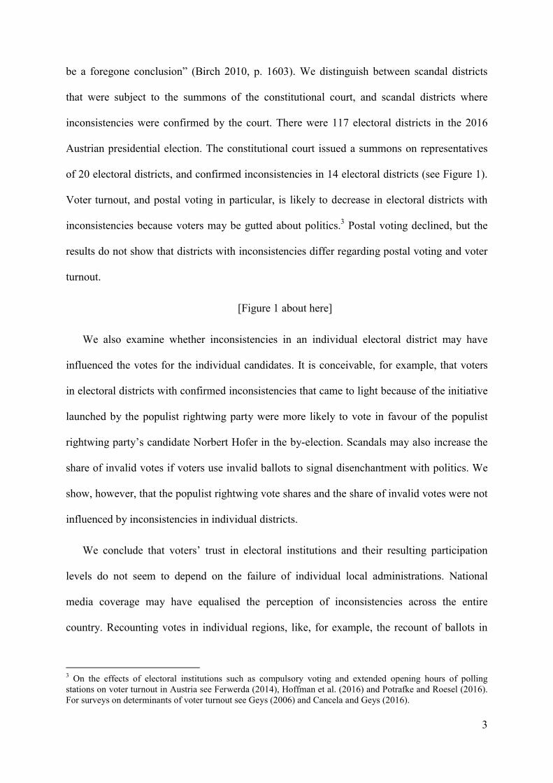
be a foregone conclusion” (Birch 2010, p. 1603). We distinguish between scandal districts
that were subject to the summons of the constitutional court, and scandal districts where
inconsistencies were confirmed by the court. There were 117 electoral districts in the 2016
Austrian presidential election. The constitutional court issued a summons on representatives
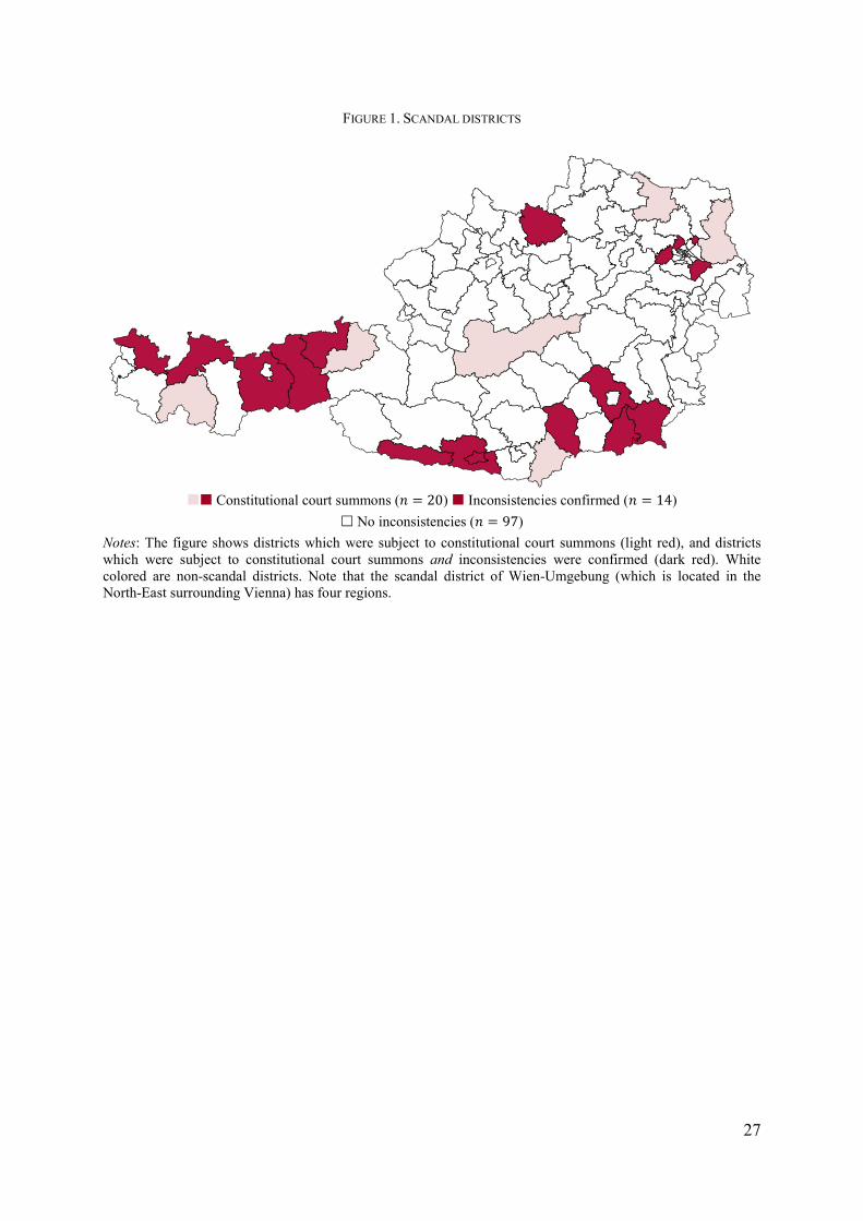
of 20 electoral districts, and confirmed inconsistencies in 14 electoral districts (see Figure 1).
Voter turnout, and postal voting in particular, is likely to decrease in electoral districts with
inconsistencies because voters may be gutted about politics.3 Postal voting declined, but the
results do not show that districts with inconsistencies differ regarding postal voting and voter
turnout.
[Figure 1 about here]
We also examine whether inconsistencies in an individual electoral district may have
influenced the votes for the individual candidates. It is conceivable, for example, that voters
in electoral districts with confirmed inconsistencies that came to light because of the initiative
launched by the populist rightwing party were more likely to vote in favour of the populist
rightwing party’s candidate Norbert Hofer in the by-election. Scandals may also increase the
share of invalid votes if voters use invalid ballots to signal disenchantment with politics. We
show, however, that the populist rightwing vote shares and the share of invalid votes were not
influenced by inconsistencies in individual districts.
We conclude that voters’ trust in electoral institutions and their resulting participation
levels do not seem to depend on the failure of individual local administrations. National
media coverage may have equalised the perception of inconsistencies across the entire
country. Recounting votes in individual regions, like, for example, the recount of ballots in
3 On the effects of electoral institutions such as compulsory voting and extended opening hours of polling stations on voter turnout in Austria see Ferwerda (2014), Hoffman et al. (2016) and Potrafke and Roesel (2016). For surveys on determinants of voter turnout see Geys (2006) and Cancela and Geys (2016).
4
Wisconsin in the course of the US presidential election 2016, are likely to impact national,
rather than specific regional voting behaviour.
2. Related Literature
2.1 Political trust and electoral outcomes
Some studies elaborate on the correlation between trust such as in international organisations
and voter turnout. Cox (2003) uses cross-sectional data on trust and voter turnout in 13
European countries. Voter turnout is for national elections and elections to the European
Parliament in the year 1999. Parliamentary trust is measured by 1999 Eurobarometer data in
which participants were asked: “For each of the following European institutions, please tell
me if you tend to trust it or tend to not trust it”. In particular, the author also uses the
percentage of respondents that expressed their trust in the European parliament. Interpersonal
trust is measured by the 1990-1993 and 1995-1997 World Values Surveys (WVS) questions:
“Generally speaking, would you say that most people can be trusted or that you can’t be too
careful in dealing with people?” The results show that interpersonal trust was not correlated
with voter turnout in elections to the national and European parliament. By contrast, political
institution trust, and especially trust in the European Parliament was significantly positively
correlated with voter turnout in elections to the European Parliament.
In Latin America, distrust in elections was huge: Carrerras and İrepoğlu (2013) use
survey data and report that about 33.2 % of Latin American respondents did not trust in
(domestic) electoral processes compared to 5 % in North American and Western Europe. The
authors also use data from the 2010 Americas Barometer, a survey “administered by the Latin
American Public Opinion Project (LAPOP) at Vanderbuilt University” (p. 614). The survey
includes respondents from 18 Latin American countries. The authors estimate a micro-
5
econometric model using a binary dependent variable measuring whether respondents voted
in the last Presidential elections. The main explanatory variable is based on the answers to the
question “To what extent to you trust elections?” This variable is categorical assuming values
between 1 and 7. The results show that respondents with low trust in elections (1) were some
3.8 percentage points less likely to participate in elections than respondents with high trust in
elections (7).
In US presidential elections over the period 1968-1996, declining political trust increased
support for the non-incumbent party, when two candidates were running. When three
candidates were running for office, however, distrustful voters were inclined to vote for the
third-party candidate, at the expense of the Republican and Democratic candidates.
Hetherington (1999) arrived at these results using micro data of the National Election Surveys
(NES). Political trust is measured by the respondents’ mean score on a four item trust index.
Political trust in government – as measured by the NES-data – was hardly correlated with
voter turnout in US presidential elections over the period 1964–1972 (Citrin 1974), and
especially in the 1972 election (Knack 1992). By contrast, trust in people was positively
correlated with voter turnout in the 1972 presidential elections (Knack 1992).
2.2 Scandals and electoral outcomes
Political scandals are expected to have electoral consequences. Voters may, for example, vote
incumbents out of office if the incumbents are accused of having violated the law or ethical
rules. Scholars examine the electoral consequences of individual political scandals such as the
MP’s 2009 expenses scandal in the United Kingdom. The research design often used is to
estimate a difference-in-differences model exploiting being involved in a scandal as
treatment. Studies compare party vote shares or voter turnout in the pre-scandal and post-
scandal elections.
6
Since 1988 MP’s in the United Kingdom have been allowed to make expenses claims to
cover, for example, the costs of running their offices or of running a second household (one
household in London and one in the home constituency). “Some seemed bizarrely out of
touch (as with the senior MP who claimed against the cost of having someone replace faulty
light bulbs)” (Pattie and Johnston 2012: 733). The scandal leaked out in May 2009 when the
newspaper the Daily Telegraph began to report about the issue, one year before the
parliamentary elections in 2010. Four studies investigate issues of electoral accountability in
the course of the scandal: Eggers (2014), Larcinese and Sircar (2017), Pattie and Johnston
(2012) and Vivyan et al. (2012).
The vote share of MPs who were implicated in the scandal was by about 2.6 percentage
points lower than the vote share of MPs who were not involved, compared to the previous
2005 parliamentary election (Eggers 2014).4 Partisanship in the electoral districts, however,
had a major impact on the extent to which voters punished MPs. Eggers (2014) exploits
variance across constituencies considering whether an individual constituency had a strong
Labour-Conservative-battleground (high partisanship); or whether a Liberal Democrat was
the main challenger to a labour or conservative politician (low partisanship) in an individual
constituency. The results show that in constituencies with low partisanship, the vote share of
MPs who were implicated in the scandal was by about 6 percentage points lower than the vote
share of MPs who were not involved. Politicians in constituencies with low partisanship were
hence relatively less punished, but were also more likely to be implicated in the scandal in the
first place.
4 The authors measure “implication in the expenses scandal based on the proportion of news stories in the Google News archive mentioning an MP and her constituency during the period between the beginning of the scandal and the 2010 election that also mention the word “expensens”” (p. 449). The author computes a continuous variable for “sinners” and “saints,” which he translates into a binary variable indicating whether an MP was implicated in the scandal.
7
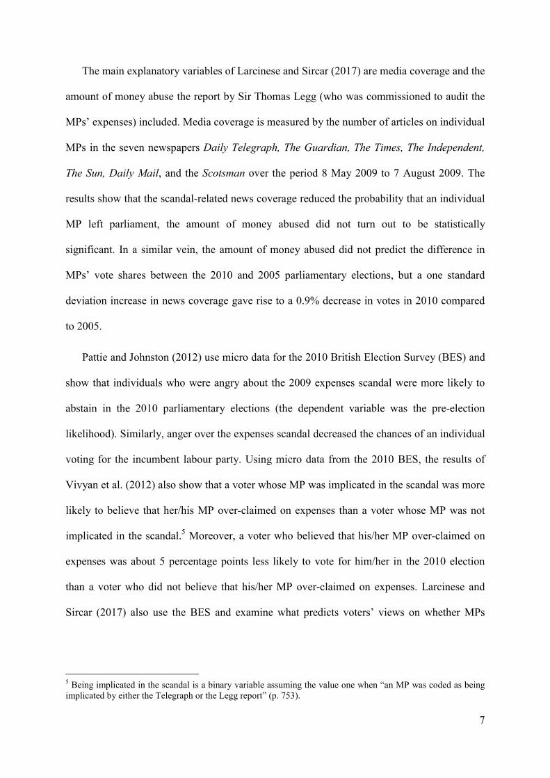
The main explanatory variables of Larcinese and Sircar (2017) are media coverage and the
amount of money abuse the report by Sir Thomas Legg (who was commissioned to audit the
MPs’ expenses) included. Media coverage is measured by the number of articles on individual
MPs in the seven newspapers Daily Telegraph, The Guardian, The Times, The Independent,
The Sun, Daily Mail, and the Scotsman over the period 8 May 2009 to 7 August 2009. The
results show that the scandal-related news coverage reduced the probability that an individual
MP left parliament, the amount of money abused did not turn out to be statistically
significant. In a similar vein, the amount of money abused did not predict the difference in
MPs’ vote shares between the 2010 and 2005 parliamentary elections, but a one standard
deviation increase in news coverage gave rise to a 0.9% decrease in votes in 2010 compared
to 2005.
Pattie and Johnston (2012) use micro data for the 2010 British Election Survey (BES) and
show that individuals who were angry about the 2009 expenses scandal were more likely to
abstain in the 2010 parliamentary elections (the dependent variable was the pre-election
likelihood). Similarly, anger over the expenses scandal decreased the chances of an individual
voting for the incumbent labour party. Using micro data from the 2010 BES, the results of
Vivyan et al. (2012) also show that a voter whose MP was implicated in the scandal was more
likely to believe that her/his MP over-claimed on expenses than a voter whose MP was not
implicated in the scandal.5 Moreover, a voter who believed that his/her MP over-claimed on
expenses was about 5 percentage points less likely to vote for him/her in the 2010 election
than a voter who did not believe that his/her MP over-claimed on expenses. Larcinese and
Sircar (2017) also use the BES and examine what predicts voters’ views on whether MPs
5 Being implicated in the scandal is a binary variable assuming the value one when “an MP was coded as being implicated by either the Telegraph or the Legg report” (p. 753).
8
over-claimed on expenses. The results show that perceived involvement of an MP increased
by about 0.07% when the money MPs were accused to have over-claimed increased by 1%.
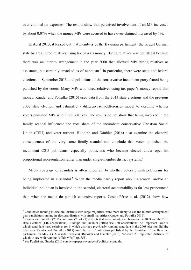
In April 2013, it leaked out that members of the Bavarian parliament (the largest German
state by area) hired relatives using tax payer’s money. Hiring relatives was not illegal because
there was an interim arrangement in the year 2000 that allowed MPs hiring relatives as
assistants, but certainly smacked as of nepotism.6 In particular, there were state and federal
elections in September 2013, and politicians of the conservative incumbent party feared being
punished by the voters. Many MPs who hired relatives using tax paper’s money repaid that
money. Kauder and Potrafke (2015) used data from the 2013 state elections and the previous
2008 state election and estimated a differences-in-differences model to examine whether
voters punished MPs who hired relatives. The results do not show that being involved in the
family scandal influenced the vote share of the incumbent conservative Christian Social
Union (CSU) and voter turnout. Rudolph and Däubler (2016) also examine the electoral
consequences of the very same family scandal and conclude that voters punished the
incumbent CSU politicians, especially politicians who became elected under open-list
proportional representation rather than under single-member district systems.7
Media coverage of scandals is often important to whether voters punish politicians for
being implicated in a scandal.8 When the media hardly report about a scandal and/or an
individual politician is involved in the scandal, electoral accountability is far less pronounced
than when the media do publish extensive reports. Costas-Pérez et al. (2012) show how
6 Candidates running in electoral districts with large majorities were more likely to use the interim arrangement than candidates running in electoral districts with small majorities (Kauder and Potrafke 2016). 7 Kauder and Potrafke (2015) use those (73 of 91) districts that were not adjusted between the 2008 and the 2013 state elections (146 observations). Rudolph and Däubler (2016) use 180 observations. An important issue is which candidate hired relatives (or in which district a previously running candidate in the 2008 election did hire relatives). Kauder and Potrafke (2015) used the list of politicians published by the President of the Bavarian parliament on May 3 (16 scandal districts). Rudolph and Däubler (2016) “observe 23 implicated districts, of which 14 are with running “affair MPs”” (p. 755). 8 See Puglisi and Snyder (2011) on newspaper coverage of political scandals.
9
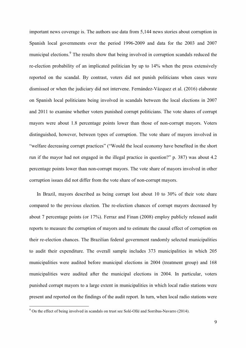
important news coverage is. The authors use data from 5,144 news stories about corruption in
Spanish local governments over the period 1996-2009 and data for the 2003 and 2007
municipal elections.9 The results show that being involved in corruption scandals reduced the
re-election probability of an implicated politician by up to 14% when the press extensively
reported on the scandal. By contrast, voters did not punish politicians when cases were
dismissed or when the judiciary did not intervene. Fernández-Vázquez et al. (2016) elaborate
on Spanish local politicians being involved in scandals between the local elections in 2007
and 2011 to examine whether voters punished corrupt politicians. The vote shares of corrupt
mayors were about 1.8 percentage points lower than those of non-corrupt mayors. Voters
distinguished, however, between types of corruption. The vote share of mayors involved in
“welfare decreasing corrupt practices” (“Would the local economy have benefited in the short
run if the mayor had not engaged in the illegal practice in question?” p. 387) was about 4.2
percentage points lower than non-corrupt mayors. The vote share of mayors involved in other
corruption issues did not differ from the vote share of non-corrupt mayors.
In Brazil, mayors described as being corrupt lost about 10 to 30% of their vote share
compared to the previous election. The re-election chances of corrupt mayors decreased by
about 7 percentage points (or 17%). Ferraz and Finan (2008) employ publicly released audit
reports to measure the corruption of mayors and to estimate the causal effect of corruption on
their re-election chances. The Brazilian federal government randomly selected municipalities
to audit their expenditure. The overall sample includes 373 municipalities in which 205
municipalities were audited before municipal elections in 2004 (treatment group) and 168
municipalities were audited after the municipal elections in 2004. In particular, voters
punished corrupt mayors to a large extent in municipalities in which local radio stations were
present and reported on the findings of the audit report. In turn, when local radio stations were
9 On the effect of being involved in scandals on trust see Solé-Ollé and Sorribas-Navarro (2014).
10
present and reported on the findings of the audit report, the re-election prospects of non-
corrupt incumbents increased.
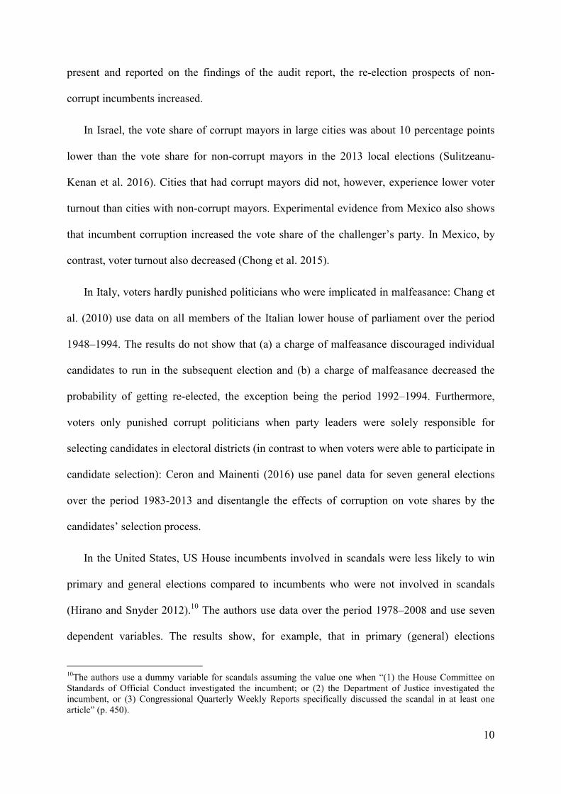
In Israel, the vote share of corrupt mayors in large cities was about 10 percentage points
lower than the vote share for non-corrupt mayors in the 2013 local elections (Sulitzeanu-
Kenan et al. 2016). Cities that had corrupt mayors did not, however, experience lower voter
turnout than cities with non-corrupt mayors. Experimental evidence from Mexico also shows
that incumbent corruption increased the vote share of the challenger’s party. In Mexico, by
contrast, voter turnout also decreased (Chong et al. 2015).
In Italy, voters hardly punished politicians who were implicated in malfeasance: Chang et
al. (2010) use data on all members of the Italian lower house of parliament over the period
1948–1994. The results do not show that (a) a charge of malfeasance discouraged individual
candidates to run in the subsequent election and (b) a charge of malfeasance decreased the
probability of getting re-elected, the exception being the period 1992–1994. Furthermore,
voters only punished corrupt politicians when party leaders were solely responsible for
selecting candidates in electoral districts (in contrast to when voters were able to participate in
candidate selection): Ceron and Mainenti (2016) use panel data for seven general elections
over the period 1983-2013 and disentangle the effects of corruption on vote shares by the
candidates’ selection process.
In the United States, US House incumbents involved in scandals were less likely to win
primary and general elections compared to incumbents who were not involved in scandals
(Hirano and Snyder 2012).10 The authors use data over the period 1978–2008 and use seven
dependent variables. The results show, for example, that in primary (general) elections
10The authors use a dummy variable for scandals assuming the value one when “(1) the House Committee on Standards of Official Conduct investigated the incumbent; or (2) the Department of Justice investigated the incumbent, or (3) Congressional Quarterly Weekly Reports specifically discussed the scandal in at least one article” (p. 450).
11
incumbents involved in scandals received about 16 (11) percent fewer votes than incumbents
who were not involved in scandals.
3. Institutional background
Austrian presidents have been elected in direct elections since 1951. The duration of their
term-in-office is six years. The president is the federal head of the state of Austria and
theoretically enjoys a great deal of power. In practice, however, the Austrian president
administrates ceremonial events such as receptions and addresses of welcome. In contrast to
the indirect presidential elections in the United States (system of electors), for example, the
Austrian president is proportionally and directly elected. A candidate needs over 50% of the
valid ballots casted nationwide to win. There are two rounds. If no candidate receives more
than 50% in the first ballot, a second (run-off) ballot is held among the two candidates that
received the most votes in the first round. Votes cast at the “regular” ballot box are collected
at the local level (Gemeinde); postal votes, by contrast, are counted at the (electoral) district
level (Bezirk), which is the upper-local administrative level. There is no information on postal
voting at the local level.
The 2016 presidential election in Austria was unique in many ways. Austrian presidents
since World War II were either members of the Social Democratic Party (SPÖ) or the
Conservative Party (ÖVP), and one president, Rudolf Kirchschläger, was crossbench (in
office over the period 1974–1986). In the first ballot of the 2016 presidential election on 24
April, however, neither a candidate of the SPÖ nor the ÖVP made it to the second ballot, but
a candidate from the populist rightwing Freedom Party (FPÖ), Norbert Hofer, and of the
Green Party (Greens), Alexander van der Bellen did. The Austrian party system has changed
dramatically as in many other western democracies in recent years. In the second ballot on 22
May 2016, the Green candidate van der Bellen won the election against the populist rightwing
12
candidate Norbert Hofer with a marginal lead of 30,863 votes (van der Bellen received 50.35
% of the votes, Hofer received 49.65%). Postal votes turned the balance in favour of van der
Bellen. Voter turnout was 72.7%.
The defeated FPÖ was concerned about inconsistencies, especially in dealing with postal
votes. As a result, the chairman of the populist rightwing FPÖ, Hans-Christian Strache, went
to the constitutional court to contest the second ballot. The constitutional court scrutinized the
constitutional complaint for about a month. On 1 July 2016, the constitutional court acceded
to the constitutional complaint because of inconsistencies. For example, postal votes must be
counted on the Monday after the election (which takes place on a Sunday) at 9 a.m. In
Bregenz, campaign workers started to count postal votes at 8 a.m. In Innsbruck-Land,
campaign workers started to count the postal votes at 9 a.m., but already opened the envelopes
of postal votes on Sunday.11 The constitutional court made clear that there was no concern
over manipulation, but the rules were broken. The inconsistencies affected 77,926 votes; an
amount of votes which may well have changed the outcome of the election, because
Alexander van der Bellen won by 30,863 votes against Norbert Hofer. The constitutional
court called for a repetition of the second ballot.
The by-election of the second ballot was scheduled to take place on 2 October 2016.
There were, however, inconsistencies with the papers for the postal votes (some of the
envelopes that were sent out to the citizens who wanted to use postal voting could not be
sealed). On 12 September 2016, the government therefore decided to postpone the by-election
of the second ballot. The by-election of the second ballot thus took place on 4 December
2016. Alexander van der Bellen won the by-election of the second ballot with 53%. Voter
turnout was 74.1%. The register of eligible voters was updated to account for mortality,
naturalization, and population passing the voting age of 16 between February 2016 and
11 See Frankfurter Allgemeine Zeitung, 02.07.2016, “Wenigstens der österreichische Wein taugt noch was”.
13
September 2016. The total electorate, however, increased only by 0.27% from 6,382,507 to
6,399,572. We do not believe that this update of the eligible voters influences our inferences.
In any event, we will also control for changes in the district electorate.
4. Empirical analysis
4.1 Identification strategy
We use a difference-in-difference approach to identify the causal effect of being a scandal
district on voter behaviour (postal voting, voter turnout, invalid voting, and candidate vote
shares). Our key identifying assumption is that scandal and non-scandal districts follow a
common trend, which would have applied in the absence of the scandal. We describe why we
believe that the common trend assumption holds.
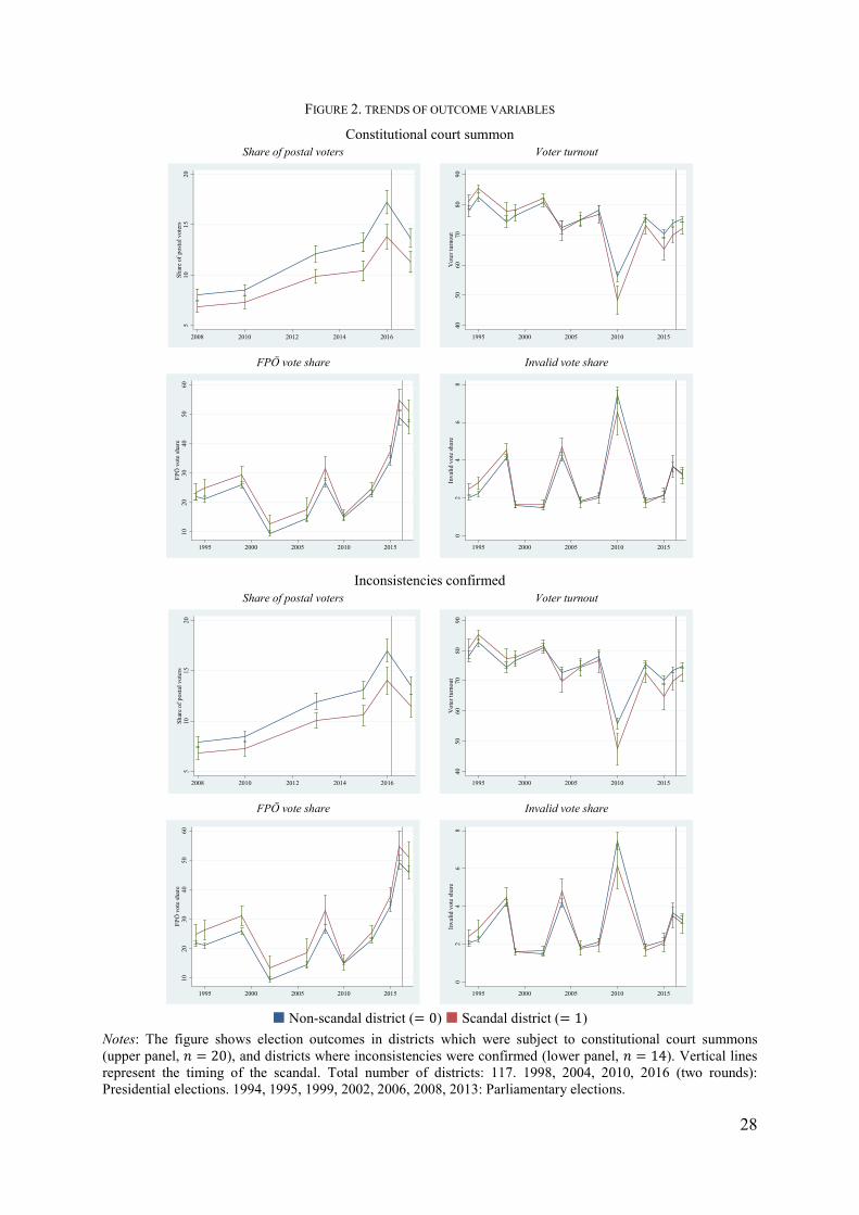
Firstly, Figure 2 suggests that there are parallel pre-scandal trends in postal voting,
voter turnout, FPÖ vote shares and invalid vote shares in the scandal and non-scandal
districts. Vertical lines describe the timing of the scandal. The upper panel compares districts
that were subject to constitutional court summons to the remaining districts, the lower panel
compares districts with confirmed inconsistencies to all other districts. Postal voting was
introduced in 2007, data are therefore available since the national election of 2008. In both
scandal and non-scandal districts, the share of voters using postal voting increased to around
15% in the first round of the 2016 presidential election. Voter turnout in nationwide elections
decreased from around 80% in the early 1990s to around 70% in 2016. The vote share of the
populist rightwing FPÖ was usually between 10% and 30% and has not differed significantly
in scandal and non-scandal districts over the last ten years. The same holds true for invalid
votes. The share of invalid votes was substantially larger in presidential elections (1998, 2004,
2010, and 2016), but did not differ among scandal and non-scandal districts. As a result, both
14
groups of districts seemed to have followed a common trend. Group mean differences are
small and even diminish when the 23 electoral districts of Vienna are excluded (see
Appendix, Figure A.1).
[Figure 2 about here]
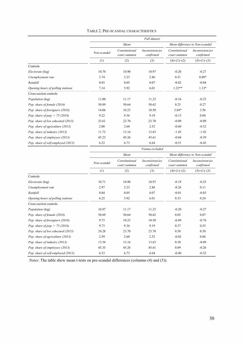
Secondly, we test whether observable pre-scandal characteristics differ across scandal
and non-scandal districts. Table 2 indicates that there were no significant differences between
non-scandal districts and districts where inconsistencies were subject to court summons
(column (4)), or where inconsistencies were confirmed (column (5)). Neither pre-scandal
electorate, rainfall nor other socio-demographic variables, e.g., the population share of female,
foreigners, elderly people, differ across district groups. The exceptions are the opening hours
of polling stations, unemployment, and the share of foreigners that are somewhat larger in
non-scandal districts. If we exclude the districts of Vienna (lower panel of Table 2), however,
these differences also lack statistical significance.
[Table 2 about here]
Thirdly, there seems to be no spatial clustering of scandal districts. Figure 1 shows that
many scandal districts are in the West (Tyrol, Vorarlberg), in the South (Carinthia, Styria),
and in the North (Upper Austria, Lower Austria) of Austria. Inconsistencies were widespread;
the FPÖ accused 97 out of 117 districts of possible manipulations.
Fourthly, the education and skills of the civil servants in the districts may have
influenced the selection into treatment. The less educated the civil servants are, the more
likely inconsistencies may be. However, differences in education between scandal and non-
scandal district administrations are unlikely. The education of civil servants is standardised in
Austria. We also do not find any evidence that failing district officials resigned in the course
of the scandals. Quite on the contrary, the district authority of Bregenz (state of Vorarlberg)
15
complained that their failing civil servants were somehow subject to “witch hunting” which
“they do not deserve”.12 Administrative abilities thus do not predict selection into treatment.
Fifthly, we examine whether the detection of inconsistencies may have been
manipulated, and consequently, have given rise to a selection into treatment. We do not
believe that there was such selection into treatment for two reasons. Members of the three
main parties (the social-democratic SPÖ, the conservative ÖVP, and the populist rightwing
FPÖ) were allowed to join the committees counting postal votes in all districts. Thus, FPÖ
district branches had the same chance in all districts to detect inconsistencies. Moreover, the
broad media coverage encouraged many advocates and party members of the FPÖ to report
inconsistencies via Facebook. FPÖ officials collected, analysed and conjoined all reports. The
complaint of the FPÖ explicitly referred to Facebook sources. Therefore, even a small number
of voters per district (e.g., in districts in which citizens hardly vote for the FPÖ) were
sufficient to enter the document for the investigation by the constitutional court.
Altogether, we believe in common trends and a selection mechanism that is orthogonal to
observable, but also to unobservable characteristics. The nationwide repetition of an election
is a unique event in Austrian history; in 1970 and 1995, national elections only had to be
repeated in individual municipalities where minor inconsistencies occurred.
4.2 Data
We use data at the level of the 117 electoral districts of Austria for the original and the
repeated second ballot of the Austrian presidential election in May and December 2016.13
Electoral districts are administrative entities for structuring the counting of votes, and of
postal votes in particular. Election data and data on the opening hours of polling stations are
12 See, Der Standard, 14.07.2016, http://derstandard.at/2000041085212/Disziplinarstellen-ermitteln-gegen-Beamte. 13 Vienna accounts for 23 of the 117 electoral districts of Austria.
16
obtained from the Austrian Federal Ministry of the Interior. We compile data on rain from the
weather website wetteronline.de. All other variables are collected from the publications of
Statistics Austria. We code scandal districts accordingly to the twitter postings and press
releases of the constitutional court.14
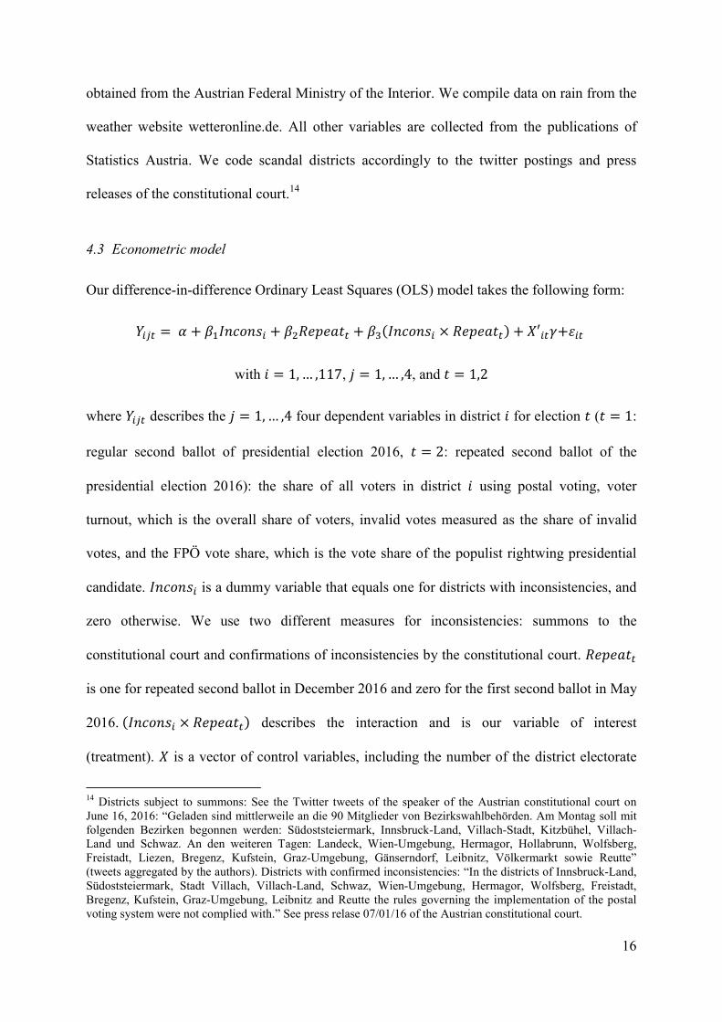
4.3 Econometric model
Our difference-in-difference Ordinary Least Squares (OLS) model takes the following form:
���� = � + ��������� + ��������� + ��(������� × �������) + �′���+���
with � = 1, … ,117, � = 1, … ,4, and � = 1,2
where ���� describes the � = 1, … ,4 four dependent variables in district � for election � (� = 1:
regular second ballot of presidential election 2016, � = 2: repeated second ballot of the
presidential election 2016): the share of all voters in district � using postal voting, voter
turnout, which is the overall share of voters, invalid votes measured as the share of invalid
votes, and the FPÖ vote share, which is the vote share of the populist rightwing presidential
candidate. ������� is a dummy variable that equals one for districts with inconsistencies, and
zero otherwise. We use two different measures for inconsistencies: summons to the
constitutional court and confirmations of inconsistencies by the constitutional court. �������
is one for repeated second ballot in December 2016 and zero for the first second ballot in May
2016. (������� × �������) describes the interaction and is our variable of interest
(treatment). � is a vector of control variables, including the number of the district electorate
14 Districts subject to summons: See the Twitter tweets of the speaker of the Austrian constitutional court on June 16, 2016: “Geladen sind mittlerweile an die 90 Mitglieder von Bezirkswahlbehörden. Am Montag soll mit folgenden Bezirken begonnen werden: Südoststeiermark, Innsbruck-Land, Villach-Stadt, Kitzbühel, Villach-Land und Schwaz. An den weiteren Tagen: Landeck, Wien-Umgebung, Hermagor, Hollabrunn, Wolfsberg, Freistadt, Liezen, Bregenz, Kufstein, Graz-Umgebung, Gänserndorf, Leibnitz, Völkermarkt sowie Reutte” (tweets aggregated by the authors). Districts with confirmed inconsistencies: “In the districts of Innsbruck-Land, Südoststeiermark, Stadt Villach, Villach-Land, Schwaz, Wien-Umgebung, Hermagor, Wolfsberg, Freistadt, Bregenz, Kufstein, Graz-Umgebung, Leibnitz and Reutte the rules governing the implementation of the postal voting system were not complied with.” See press relase 07/01/16 of the Austrian constitutional court.
17
(log), the amount of rain in the district capital city at the election day, the district average in
the opening hours of polling stations that differ substantially across Austria, and the
unemployment rate. We estimate the difference-in-differences model with standard errors
robust to heteroskedasticity (Huber-White sandwich standard errors – see Huber 1967, White
1980).
5. Results
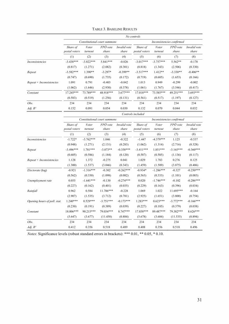
5.1 Baseline
The baseline results do not show that voting behaviour changed across scandal and non-
scandal districts in the repeated ballot. The upper panel of Table 3 shows the difference-in-
differences results for a specification excluding control variables. Columns (1) to (4) refer to
districts that were subject to summons to the constitutional court, columns (5) to (8) refer to
confirmed inconsistencies by the constitutional court. We observe significant differences
across scandal and non-scandal districts in terms of postal voting, voter turnout and FPÖ vote
shares (���������������). We also find that all outcome variables change from the regular to
the repeated ballot. For example, voter turnout increased by about 1.4 percentage points on
average (������), and FPÖ vote shares decreased by about 3.3 percentage points. The
interaction effect of ��������������� and ������ (treatment effect), however, does not turn
out to be statistically significant in any specification.
We include several control variables (lower panel of Table 3). Voter turnout and invalid
voting decrease in the size of the electorate, and in unemployment rates. Rainfall was
associated with a higher FPÖ vote shares, but rain was fairly rare on the election day of the
regular and on the repeated election. The longer opening hours of polling stations were
associated with decreases in populist rightwing and invalid voting, as well as with increases in
18
voter turnout and, somewhat counterintuitively, increases in the share of postal votes.
Including/excluding individual control variables does not change the inferences regarding the
scandal district effects.
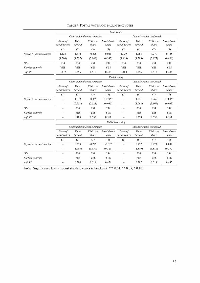
5.2 Postal votes and ballot box votes
We distinguish between different ways to cast the ballot: postal voting and “regular” voting at
the ballot box. The center and lower panel of Table 4 show that effects are similar for postal
votes and ballot box votes. None of the effects turns out to be significant. The sole exception
is invalid postal voting: in scandal districts, the share of invalid postal votes is about 7.6
percentage points higher than in non-scandal districts. It is, however, unclear why postal
voters in scandal districts should be more inclined towards invalid voting than in non-scandal
districts. We believe that this effect is more likely to be a result of behavioural changes in
district administrations. District administrations tainted by scandal may have payed even more
attention to correct ballots in the repeated by-election to avoid future accusations. Thus,
scandal district administrations qualified more questionable votes to be invalid than non-
scandal district administrations. If this is true, more invalid votes may result from the more
careful counting of votes, rather than of from a change in voters’ behaviour.
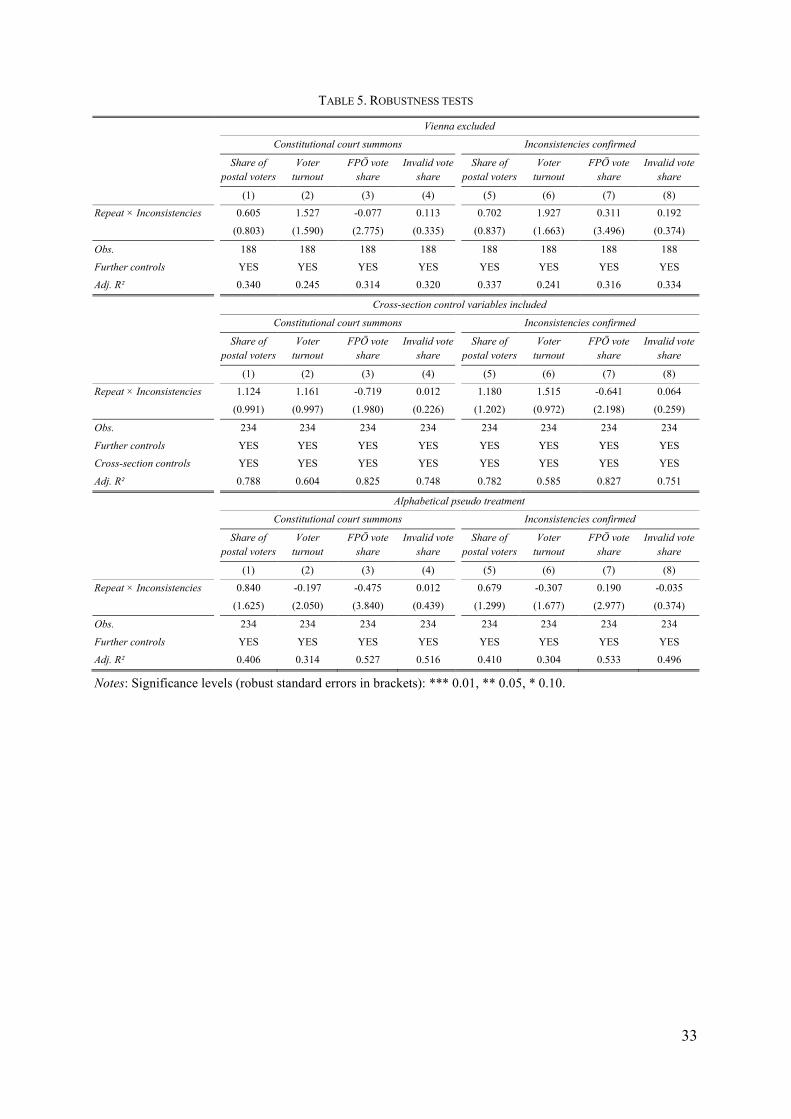
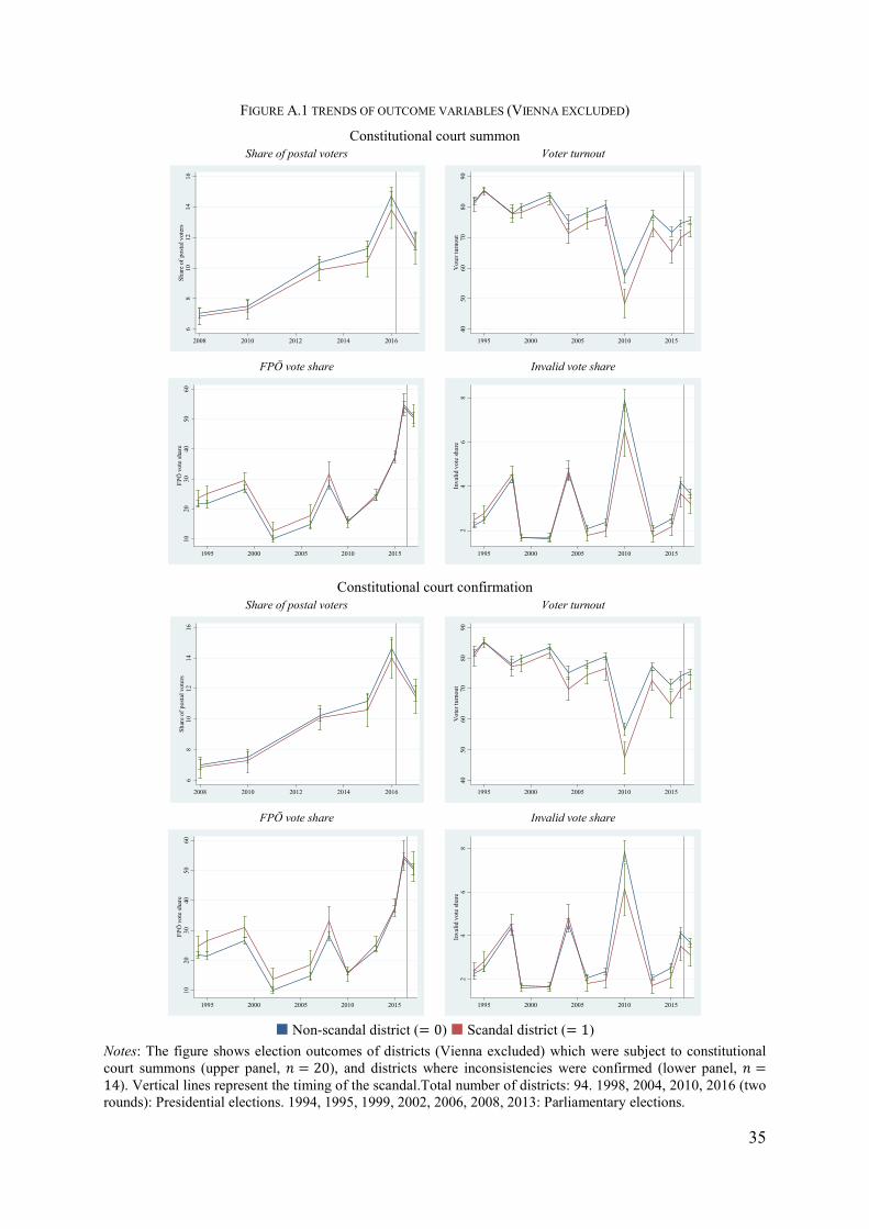
5.3 Robustness tests
We test whether the results are robust in several ways. We exclude the 23 electoral districts of
Vienna. The Austrian capital of Vienna differs from the more rural parts of Austria. For
example, postal voting is more common in Vienna than in the rest of the country. Figure A.1
in the Appendix indicates that the assumption of common trends of scandal and non-scandal
districts is even more likely to be fulfilled when we exclude Vienna. The upper panel in Table
5 shows the results. Again, none of the coefficients of the treatment effect turns out to be
statistically significant.
19
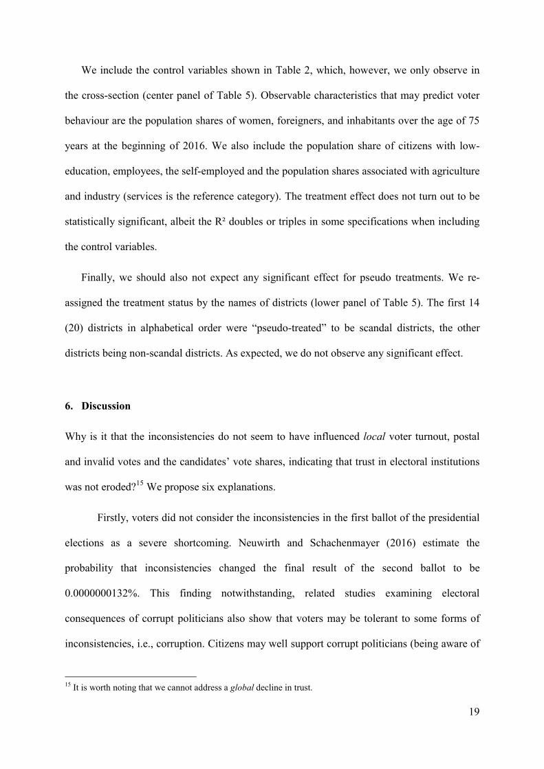
We include the control variables shown in Table 2, which, however, we only observe in
the cross-section (center panel of Table 5). Observable characteristics that may predict voter
behaviour are the population shares of women, foreigners, and inhabitants over the age of 75
years at the beginning of 2016. We also include the population share of citizens with low-
education, employees, the self-employed and the population shares associated with agriculture
and industry (services is the reference category). The treatment effect does not turn out to be
statistically significant, albeit the R² doubles or triples in some specifications when including
the control variables.
Finally, we should also not expect any significant effect for pseudo treatments. We re-
assigned the treatment status by the names of districts (lower panel of Table 5). The first 14
(20) districts in alphabetical order were “pseudo-treated” to be scandal districts, the other
districts being non-scandal districts. As expected, we do not observe any significant effect.
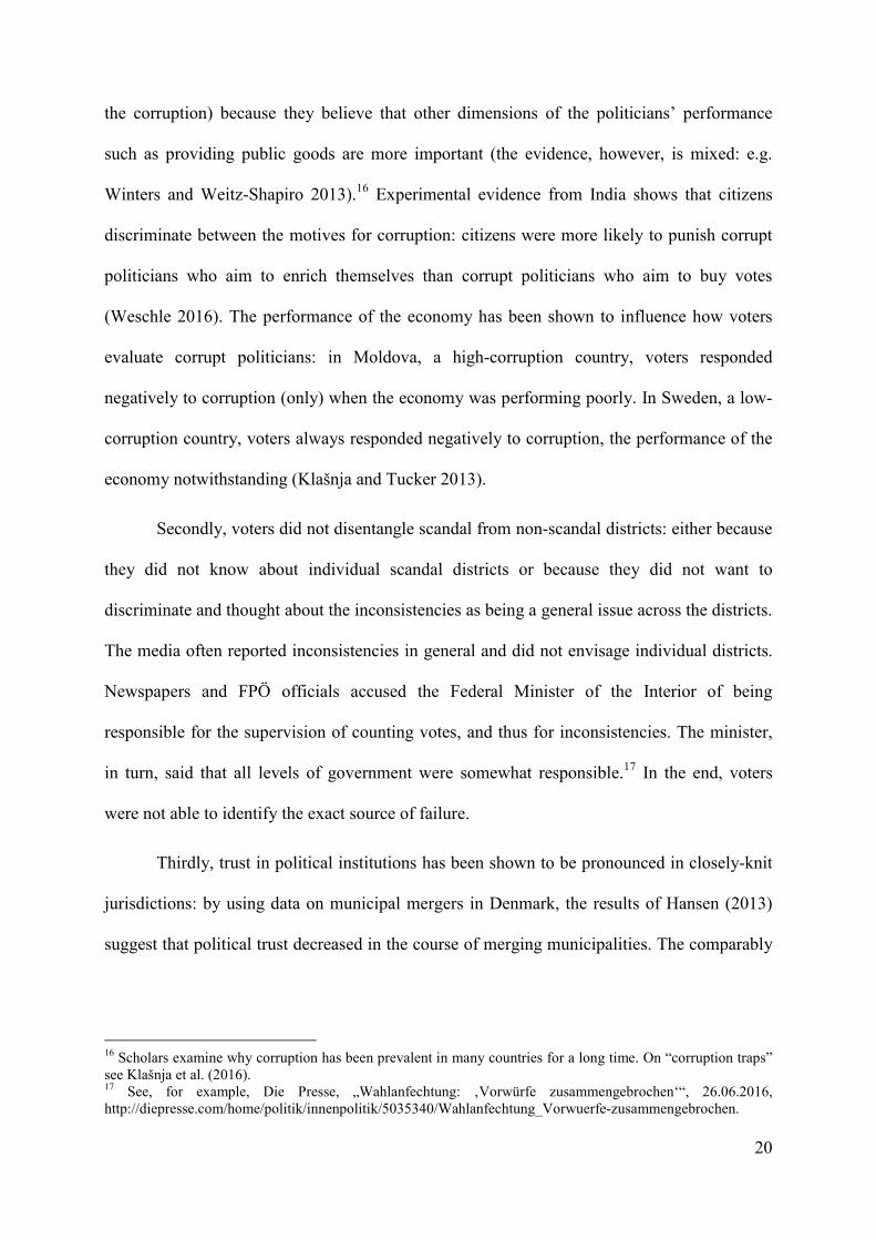
6. Discussion
Why is it that the inconsistencies do not seem to have influenced local voter turnout, postal
and invalid votes and the candidates’ vote shares, indicating that trust in electoral institutions
was not eroded?15 We propose six explanations.
Firstly, voters did not consider the inconsistencies in the first ballot of the presidential
elections as a severe shortcoming. Neuwirth and Schachenmayer (2016) estimate the
probability that inconsistencies changed the final result of the second ballot to be
0.0000000132%. This finding notwithstanding, related studies examining electoral
consequences of corrupt politicians also show that voters may be tolerant to some forms of
inconsistencies, i.e., corruption. Citizens may well support corrupt politicians (being aware of
15 It is worth noting that we cannot address a global decline in trust.
20
the corruption) because they believe that other dimensions of the politicians’ performance
such as providing public goods are more important (the evidence, however, is mixed: e.g.
Winters and Weitz-Shapiro 2013).16 Experimental evidence from India shows that citizens
discriminate between the motives for corruption: citizens were more likely to punish corrupt
politicians who aim to enrich themselves than corrupt politicians who aim to buy votes
(Weschle 2016). The performance of the economy has been shown to influence how voters
evaluate corrupt politicians: in Moldova, a high-corruption country, voters responded
negatively to corruption (only) when the economy was performing poorly. In Sweden, a low-
corruption country, voters always responded negatively to corruption, the performance of the
economy notwithstanding (Klašnja and Tucker 2013).
Secondly, voters did not disentangle scandal from non-scandal districts: either because
they did not know about individual scandal districts or because they did not want to
discriminate and thought about the inconsistencies as being a general issue across the districts.
The media often reported inconsistencies in general and did not envisage individual districts.
Newspapers and FPÖ officials accused the Federal Minister of the Interior of being
responsible for the supervision of counting votes, and thus for inconsistencies. The minister,
in turn, said that all levels of government were somewhat responsible.17 In the end, voters
were not able to identify the exact source of failure.
Thirdly, trust in political institutions has been shown to be pronounced in closely-knit
jurisdictions: by using data on municipal mergers in Denmark, the results of Hansen (2013)
suggest that political trust decreased in the course of merging municipalities. The comparably
16 Scholars examine why corruption has been prevalent in many countries for a long time. On “corruption traps” see Klašnja et al. (2016). 17 See, for example, Die Presse, „Wahlanfechtung: ‚Vorwürfe zusammengebrochen‘“, 26.06.2016, http://diepresse.com/home/politik/innenpolitik/5035340/Wahlanfechtung_Vorwuerfe-zusammengebrochen.
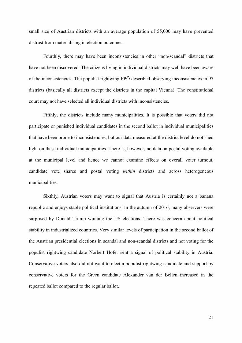
21
small size of Austrian districts with an average population of 55,000 may have prevented
distrust from materialising in election outcomes.
Fourthly, there may have been inconsistencies in other “non-scandal” districts that
have not been discovered. The citizens living in individual districts may well have been aware
of the inconsistencies. The populist rightwing FPÖ described observing inconsistencies in 97
districts (basically all districts except the districts in the capital Vienna). The constitutional
court may not have selected all individual districts with inconsistencies.
Fifthly, the districts include many municipalities. It is possible that voters did not
participate or punished individual candidates in the second ballot in individual municipalities
that have been prone to inconsistencies, but our data measured at the district level do not shed
light on these individual municipalities. There is, however, no data on postal voting available
at the municipal level and hence we cannot examine effects on overall voter turnout,
candidate vote shares and postal voting within districts and across heterogeneous
municipalities.
Sixthly, Austrian voters may want to signal that Austria is certainly not a banana
republic and enjoys stable political institutions. In the autumn of 2016, many observers were
surprised by Donald Trump winning the US elections. There was concern about political
stability in industrialized countries. Very similar levels of participation in the second ballot of
the Austrian presidential elections in scandal and non-scandal districts and not voting for the
populist rightwing candidate Norbert Hofer sent a signal of political stability in Austria.
Conservative voters also did not want to elect a populist rightwing candidate and support by
conservative voters for the Green candidate Alexander van der Bellen increased in the
repeated ballot compared to the regular ballot.
22
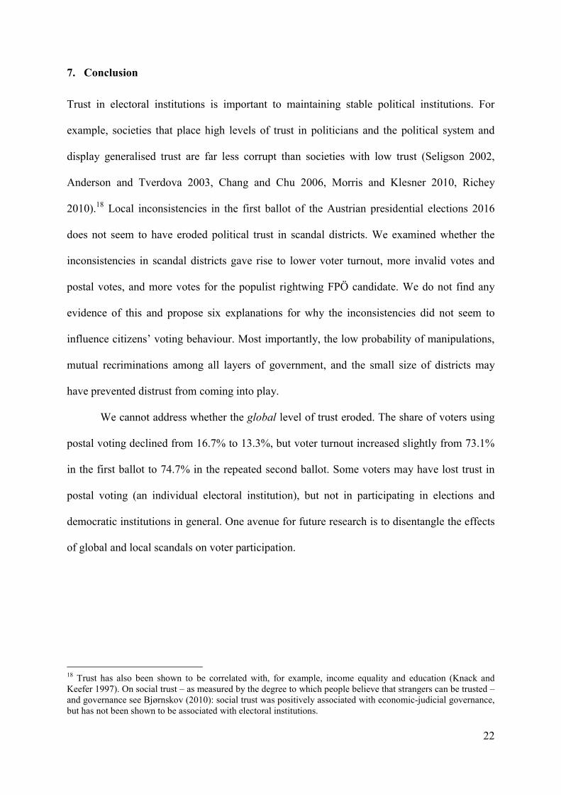
7. Conclusion
Trust in electoral institutions is important to maintaining stable political institutions. For
example, societies that place high levels of trust in politicians and the political system and
display generalised trust are far less corrupt than societies with low trust (Seligson 2002,
Anderson and Tverdova 2003, Chang and Chu 2006, Morris and Klesner 2010, Richey
2010).18 Local inconsistencies in the first ballot of the Austrian presidential elections 2016
does not seem to have eroded political trust in scandal districts. We examined whether the
inconsistencies in scandal districts gave rise to lower voter turnout, more invalid votes and
postal votes, and more votes for the populist rightwing FPÖ candidate. We do not find any
evidence of this and propose six explanations for why the inconsistencies did not seem to
influence citizens’ voting behaviour. Most importantly, the low probability of manipulations,
mutual recriminations among all layers of government, and the small size of districts may
have prevented distrust from coming into play.
We cannot address whether the global level of trust eroded. The share of voters using
postal voting declined from 16.7% to 13.3%, but voter turnout increased slightly from 73.1%
in the first ballot to 74.7% in the repeated second ballot. Some voters may have lost trust in
postal voting (an individual electoral institution), but not in participating in elections and
democratic institutions in general. One avenue for future research is to disentangle the effects
of global and local scandals on voter participation.
18 Trust has also been shown to be correlated with, for example, income equality and education (Knack and Keefer 1997). On social trust – as measured by the degree to which people believe that strangers can be trusted – and governance see Bjørnskov (2010): social trust was positively associated with economic-judicial governance, but has not been shown to be associated with electoral institutions.
23
References
Anderson, C. J., Tverdova, Y. V. 2003. Corruption, political allegiances, and attitudes toward
government in contemporary democracies. American Journal of Political Science 47,
91-109.
Birch, S., 2010. Perceptions of electoral fairness and voter turnout. Comparative Political
Studies 43, 1601-1622.
Bjørnskov, C., 2010. How does social trust lead to better governance? An attempt to separate
electoral and bureaucratic mechanisms. Public Choice 144, 323-346.
Cancela, J., Geys, B., 2016. Explaining voter turnout: A meta-analysis of national and
subnational elections. Electoral Studies 42, 264-275.
Carreras, M., İrepoğlu, Y., 2013. Trust in elections, vote buying, and turnout in Latin
America. Electoral Studies 32, 609-619.
Ceron, A., Mainenti, M.., 2016. When rotten apples spoil the ballot: The conditional effect of
corruption charges on parties’ vote shares. International Political Science Review,
forthcoming.
Chang, E. C. C., Chu, Y. 2006. Corruption and trust: Exceptionalism in Asian democracies?
Journal of Politics 68, 259-271.
Chang, E. C. C., Golden, M. A., Hill, S. J. 2010. Legislative malfeasance and political
accountability. World Politics 62, 177-220.
Chong, A., de la O, A., Karlan, D., Wantchekon. L. 2015. Does corruption information inspire
the fight or quash the hope? A field experiment in Mexico on voter turnout, choice and
party identification. Journal of Politics 77, 55-71.
Citrin, J., 1974. Comment: the political relevance of trust in government. American Political
Science Review 68, 973-988.
Costas-Pérez, E., Solé-Ollé, A., Sorribas-Navarro, P. 2012. Corruption scandals, voter
information, and accountability. European Journal of Political Economy 28, 469-484.
Cox, M., 2003. Partisanship and electoral accountability: Evidence from the UK expenses
scandal. Journal of Common Market Studies 41, 757-770.
Eggers, A., 2014. Partisanship and electoral accountability: Evidence from the UK expenses
scandal. Quarterly Journal of Political Science 9, 441-472.
24
Ferraz, C., Finan, F. 2008. Exposing corrupt politicians: The effects of Brazil’s publicly
released audits on electoral outcomes. Quarterly Journal of Economics 123, 703-745.
Fernández-Vázquez, P., Barberá, P., Rivero, G. 2016. Rooting out corruption or rooting for
corruption? The heterogenous electoral consequences of scandals, Political Science
Research and Methods 4, 379-397.
Ferwerda, J., 2014. Electoral consequences of declining participation: A natural experiment in
Austria. Electoral Studies 35, 242-252.
Geys, B., 2006. Explaining voter turnout: A review of aggregate-level research. Electoral
Studies 25, 637-663.
Hansen, S. W., 2013. Polity size and local political trust: A quasi-experiment using municipal
mergers in Denmark. Scandinavian Political Studies 36, 43-66.
Hetherington, M. J., 1999. The effect of political trust on the Presidential vote, 1986-96.
American Political Science Review 93, 311-326.
Hirano, S., Snyder, J. M. Jr. 2012. What happens to incumbents in scandals? Quarterly
Journal of Political Science 7, 447-456.
Hoffman, M., Léon, G., Lombardi, M., 2016. Compulsory voting, turnout, and government
spending: Evidence from Austria. Journal of Public Economics, forthcoming.
Huber, P. J., 1967. The behavior of maximum likelihood estimates under nonstandard
conditions. Proceedings of the Fifth Berkeley Symposium on Mathematical Statistics
and Probability, 221-233.
Kauder, B., Potrafke, N., 2015. Just hire your spouse! Evidence from a political scandal in
Bavaria. European Journal of Political Economy 38, 42-54.
Kauder, B., Potrafke, N., 2016. Supermajorities and political rent extraction. Kyklos 69, 65-
81.
Klašnja, M., Tucker, J. A. 2013. The economy, corruption, and the vote: Evidence from
experiments in Sweden and Moldova, Electoral Studies 32, 536-543.
Klašnja, M., Little, A. T., Tucker, J. A. 2016. Political corruption traps. Political Science
Research and Methods, forthcoming.
Knack, S., 1992. Civic norms, social sanctions, and voter turnout. Rationality and Society 4,
133-156.
25
Knack, S., Keefer, P. 1997. Does social capital has an economic payoff? A cross-country
investigation. Quarterly Journal of Economics 52, 1251-1287.
Larcinese, V., Sircar, I. 2017. Crime and punishment the British Way: Accountability
channels following the MPs’ expenses scandal, European Journal of Political
Economy, forthcoming.
Morris, S. D., Klesner, J. L., 2010. Corruption and trust: Theoretical considerations and
evidence from Mexico. Comparative Political Studies 43, 1258-1285.
Neuwirth E., Schachenmayer W., 2016. Eine Mathematik-Lektion für den VfGH. Falter
36/16, 14-15.
Pattie, C., Johnston, R. 2012. The electoral impact of the UK 2009 MP’s expenses scandal.
Political Studies 60, 730-750.
Potrafke, N., Roesel, F. 2016. Opening hours of polling stations and voter turnout: Evidence
from a natural experiment, CESifo Working Paper 6036.
Puglisi, R., Snyder, J. M., Jr., 2011. Newspaper coverage of political scandals. Journal of
Politics 73, 931-950.
Richey, S., 2010. The impact of corruption on social trust. American Politics Research 38,
676-690.
Rudolph, L., Däubler, T., 2016. Holding individual representative accountable: the role of
electoral systems. Journal of Politics 78, 746-762.
Seligson, M. A., 2002. The impact of corruption on regime legitimacy: a comparative study of
four Latin American countries. Journal of Politics 64, 408-432.
Solé-Ollé, A., Sorribas-Navarro, P. 2014. Does corruption erode trust in government?
Evidence from a recent surge of local scandals in Spain, CESifo Working Paper 4888.
Sulitzeanu-Kenan, R., Dotan, Y., Yair, O. 2016. Judicial anti-corruption enforcement can
enhance electoral accountability, Hebrew University of Jerusalem Legal Research
Paper No. 16-31.
Vivyan, N., Wagner, M., Tarlov, J. 2012. Representative misconduct, voter perceptions and
accountability: Evidence from the 2009 House of Commons expenses scandal,
Electoral Studies 31, 750-763.
26
Weitz-Shapiro, R. 2012. What wins votes: why some politicians opt out of clientism.
American Journal of Political Science 56, 568-583.
Weschle, S., 2016. Punishing personal and electoral corruption: Experimental evidence from
India. Research and Politics 16, 1-6.
White, H., 1980. A heteroskedasticity-consistent covariance matrix estimator and a direct test
for heteroskedasticity. Econometrica 48, 817-838.
Winters, M. S., Weitz-Shapiro, R. 2013. Corruption as a self-fulfilling prophecy: Evidence
from a survey experiment in Costa Rica. Comparative Politics 45, 418-436.
27
FIGURE 1. SCANDAL DISTRICTS
Constitutional court summons (� = 20) Inconsistencies confirmed (� = 14)
No inconsistencies (� = 97)
Notes: The figure shows districts which were subject to constitutional court summons (light red), and districts which were subject to constitutional court summons and inconsistencies were confirmed (dark red). White colored are non-scandal districts. Note that the scandal district of Wien-Umgebung (which is located in the North-East surrounding Vienna) has four regions.
28
FIGURE 2. TRENDS OF OUTCOME VARIABLES
Constitutional court summon Share of postal voters
Voter turnout
FPÖ vote share
Invalid vote share
Inconsistencies confirmed Share of postal voters
Voter turnout
FPÖ vote share
Invalid vote share
Non-scandal district (= 0) Scandal district (= 1)
Notes: The figure shows election outcomes in districts which were subject to constitutional court summons (upper panel, � = 20), and districts where inconsistencies were confirmed (lower panel, � = 14). Vertical lines represent the timing of the scandal. Total number of districts: 117. 1998, 2004, 2010, 2016 (two rounds): Presidential elections. 1994, 1995, 1999, 2002, 2006, 2008, 2013: Parliamentary elections.
510
1520
Sh
are
of p
osta
l vo
ters
2008 2010 2012 2014 2016
4050
6070
8090
Vo
ter
turn
out
1995 2000 2005 2010 2015
1020
3040
5060
FP
Ö v
ote
shar
e
1995 2000 2005 2010 2015
02
46
8In
val
id v
ote
shar
e
1995 2000 2005 2010 2015
510
1520
Sh
are
of p
osta
l vo
ters
2008 2010 2012 2014 2016
4050
6070
8090
Vo
ter
turn
out
1995 2000 2005 2010 2015
1020
3040
5060
FP
Ö v
ote
shar
e
1995 2000 2005 2010 2015
02
46
8In
val
id v
ote
sh
are
1995 2000 2005 2010 2015
29
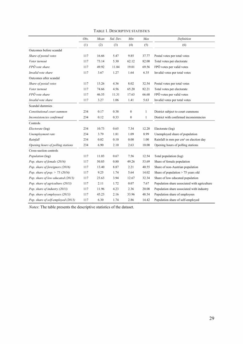
TABLE 1. DESCRIPTIVE STATISTICS
Obs. Mean Std. Dev. Min Max Definition
(1) (2) (3) (4) (5) (6)
Outcomes before scandal
Share of postal votes 117 16.66 5.47 9.85 37.77 Postal votes per total votes
Voter turnout 117 73.14 5.30 62.12 82.00 Total votes per electorate
FPÖ vote share 117 49.92 11.84 19.01 69.56 FPÖ votes per valid votes
Invalid vote share 117 3.67 1.27 1.64 6.35 Invalid votes per total votes
Outcomes after scandal
Share of postal votes 117 13.26 4.36 8.02 32.54 Postal votes per total votes
Voter turnout 117 74.66 4.56 65.20 82.21 Total votes per electorate
FPÖ vote share 117 46.55 11.31 17.63 66.68 FPÖ votes per valid votes
Invalid vote share 117 3.27 1.06 1.41 5.63 Invalid votes per total votes
Scandal dummies
Constitutional court summon 234 0.17 0.38 0 1 District subject to court cummons
Inconsistencies confirmed 234 0.12 0.33 0 1 District with confirmed inconsistencies
Controls
Electorate (log) 234 10.73 0.65 7.34 12.20 Electorate (log)
Unemployment rate 234 3.79 1.81 1.09 8.99 Unemployed share of population
Rainfall 234 0.02 0.10 0.00 1.00 Rainfall in mm per cm² on election day
Opening hours of polling stations 234 6.90 2.10 2.63 10.00 Opening hours of polling stations
Cross-section controls
Population (log) 117 11.03 0.67 7.56 12.54 Total population (log)
Pop. share of female (2016) 117 50.85 0.80 49.26 53.69 Share of female population
Pop. share of foreigners (2016) 117 13.40 8.87 2.21 40.55 Share of non-Austrian population
Pop. share of pop. > 75 (2016) 117 9.25 1.74 5.64 14.02 Share of population > 75 years old
Pop. share of low educated (2013) 117 23.63 3.94 12.67 32.34 Share of low educated population
Pop. share of agriculture (2013) 117 2.11 1.72 0.07 7.67 Population share associated with agriculture
Pop. share of industry (2013) 117 11.96 4.23 2.36 20.08 Population share associated with industry
Pop. share of employees (2013) 117 45.23 2.16 33.96 48.54 Population share of employees
Pop. share of self-employed (2013) 117 6.30 1.74 2.86 14.42 Population share of self-employed
Notes: The table presents the descriptive statistics of the dataset.
30
TABLE 2. PRE-SCANDAL CHARACTERISTICS
Full dataset
Mean Mean difference to Non-scandal
Non-scandal Constitutional
court summon
Inconsistencies
confirmed
Constitutional
court summon
Inconsistencies
confirmed
(1) (2) (3) (4)=(1)–(2) (5)=(1)–(3)
Controls
Electorate (log) 10.70 10.90 10.97 -0.20 -0.27
Unemployment rate 3.74 3.23 2.86 0.51 0.88*
Rainfall 0.03 0.05 0.07 -0.02 -0.04
Opening hours of polling stations 7.14 5.92 6.01 1.22** 1.13*
Cross-section controls
Population (log) 11.00 11.17 11.23 -0.16 -0.23
Pop. share of female (2016) 50.89 50.64 50.62 0.25 0.27
Pop. share of foreigners (2016) 14.06 10.23 10.50 3.84* 3.56
Pop. share of pop. > 75 (2016) 9.22 9.36 9.19 -0.13 0.04
Pop. share of low educated (2013) 23.61 23.70 23.70 -0.09 -0.09
Pop. share of agriculture (2013) 2.00 2.60 2.52 -0.60 -0.52
Pop. share of industry (2013) 11.72 13.16 13.63 -1.45 -1.92
Pop. share of employees (2013) 45.22 45.26 45.61 -0.04 -0.39
Pop. share of self-employed (2013) 6.22 6.73 6.64 -0.51 -0.43
Vienna excluded
Mean Mean difference to Non-scandal
Non-scandal Constitutional
court summon
Inconsistencies
confirmed
Constitutional
court summon
Inconsistencies
confirmed
(1) (2) (3) (4)=(1)–(2) (5)=(1)–(3)
Controls
Electorate (log) 10.71 10.90 10.97 -0.19 -0.25
Unemployment rate 2.97 3.23 2.86 -0.26 0.11
Rainfall 0.04 0.05 0.07 -0.01 -0.03
Opening hours of polling stations 6.25 5.92 6.01 0.33 0.24
Cross-section controls
Population (log) 10.97 11.17 11.23 -0.20 -0.27
Pop. share of female (2016) 50.69 50.64 50.62 0.05 0.07
Pop. share of foreigners (2016) 9.73 10.23 10.50 -0.49 -0.76
Pop. share of pop. > 75 (2016) 9.73 9.36 9.19 0.37 0.55
Pop. share of low educated (2013) 24.28 23.70 23.70 0.58 0.58
Pop. share of agriculture (2013) 2.59 2.60 2.52 -0.02 0.06
Pop. share of industry (2013) 13.54 13.16 13.63 0.38 -0.09
Pop. share of employees (2013) 45.35 45.26 45.61 0.09 -0.26
Pop. share of self-employed (2013) 6.33 6.73 6.64 -0.40 -0.32
Notes: The table show mean t-tests on pre-scandal differences (columns (4) and (5)).
31
TABLE 3. BASELINE RESULTS
No controls
Constitutional court summons Inconsistencies confirmed
Share of
postal voters
Voter
turnout
FPÖ vote
share
Invalid vote
share
Share of
postal voters
Voter
turnout
FPÖ vote
share
Invalid vote
share
(1) (2) (3) (4) (5) (6) (7) (8)
Inconsistencies -3.438*** -3.822*** 5.841*** -0.026 -3.017*** -3.757*** 5.562** -0.178
(0.817) (1.271) (2.082) (0.301) (0.818) (1.343) (2.506) (0.330)
Repeat -3.582*** 1.390** -3.297* -0.399** -3.517*** 1.412** -3.330** -0.406**
(0.747) (0.690) (1.735) (0.172) (0.719) (0.685) (1.653) (0.166)
Repeat × Inconsistencies 1.091 0.791 -0.403 -0.042 1.013 0.949 -0.299 -0.002
(1.062) (1.646) (2.930) (0.378) (1.061) (1.767) (3.546) (0.417)
Constant 17.245*** 73.789*** 48.918*** 3.677*** 17.018*** 73.585*** 49.251*** 3.693***
(0.583) (0.519) (1.256) (0.131) (0.561) (0.517) (1.197) (0.127)
Obs. 234 234 234 234 234 234 234 234
Adj. R² 0.152 0.091 0.054 0.030 0.132 0.070 0.044 0.032
Controls included
Constitutional court summons Inconsistencies confirmed
Share of
postal voters
Voter
turnout
FPÖ vote
share
Invalid vote
share
Share of
postal voters
Voter
turnout
FPÖ vote
share
Invalid vote
share
(1) (2) (3) (4) (5) (6) (7) (8)
Inconsistencies -1.722* -3.762*** 1.046 -0.322 -1.447 -4.379*** 1.125 -0.537
(0.948) (1.271) (2.131) (0.283) (1.062) (1.314) (2.716) (0.328)
Repeat -3.496*** 1.781*** -3.073** -0.358*** -3.411*** 1.851*** -3.165*** -0.360***
(0.605) (0.586) (1.184) (0.120) (0.587) (0.585) (1.136) (0.117)
Repeat × Inconsistencies 1.128 1.372 -0.275 0.041 1.029 1.783 0.276 0.125
(1.300) (1.537) (3.046) (0.343) (1.459) (1.589) (3.875) (0.406)
Electorate (log) -0.921 -1.316*** -0.302 -0.262*** -0.934* -1.286*** -0.327 -0.250***
(0.562) (0.330) (1.098) (0.082) (0.563) (0.333) (1.101) (0.083)
Unemployment rate 0.055 -1.641*** -0.130 -0.274*** 0.020 -1.746*** -0.102 -0.286***
(0.227) (0.162) (0.401) (0.035) (0.229) (0.163) (0.396) (0.034)
Rainfall 0.962 0.584 11.786*** -0.228 1.069 1.022 11.695*** -0.164
(2.907) (1.535) (3.712) (0.781) (2.925) (1.651) (3.800) (0.754)
Opening hours of poll. stat. 1.240*** 0.529*** -3.751*** -0.173*** 1.283*** 0.623*** -3.772*** -0.166***
(0.230) (0.191) (0.389) (0.039) (0.227) (0.185) (0.379) (0.038)
Constant 18.006*** 90.215*** 79.034*** 8.747*** 17.858*** 89.487*** 79.382*** 8.626***
(5.647) (3.677) (11.450) (0.884) (5.678) (3.684) (11.535) (0.894)
Obs. 234 234 234 234 234 234 234 234
Adj. R² 0.412 0.356 0.518 0.489 0.408 0.356 0.518 0.496
Notes: Significance levels (robust standard errors in brackets): *** 0.01, ** 0.05, * 0.10.
32
TABLE 4. POSTAL VOTES AND BALLOT BOX VOTES
Total voting
Constitutional court summons Inconsistencies confirmed
Share of
postal voters
Voter
turnout
FPÖ vote
share
Invalid vote
share
Share of
postal voters
Voter
turnout
FPÖ vote
share
Invalid vote
share
(1) (2) (3) (4) (5) (6) (7) (8)
Repeat × Inconsistencies 1.128 1.372 -0.275 0.041 1.029 1.783 0.276 0.125
(1.300) (1.537) (3.046) (0.343) (1.459) (1.589) (3.875) (0.406)
Obs. 234 234 234 234 234 234 234 234
Further controls YES YES YES YES YES YES YES YES
Adj. R² 0.412 0.356 0.518 0.489 0.408 0.356 0.518 0.496
Postal voting
Constitutional court summons Inconsistencies confirmed
Share of
postal voters
Voter
turnout
FPÖ vote
share
Invalid vote
share
Share of
postal voters
Voter
turnout
FPÖ vote
share
Invalid vote
share
(1) (2) (3) (4) (5) (6) (7) (8)
Repeat × Inconsistencies – 1.019 -0.369 0.079** – 1.011 0.265 0.088**
– (0.951) (2.521) (0.035) – (1.068) (3.167) (0.039)
Obs. – 234 234 234 – 234 234 234
Further controls – YES YES YES – YES YES YES
Adj. R² – 0.403 0.535 0.561 – 0.398 0.536 0.561
Ballot box voting
Constitutional court summons Inconsistencies confirmed
Share of
postal voters
Voter
turnout
FPÖ vote
share
Invalid vote
share
Share of
postal voters
Voter
turnout
FPÖ vote
share
Invalid vote
share
(1) (2) (3) (4) (5) (6) (7) (8)
Repeat × Inconsistencies – 0.353 -0.279 -0.037 – 0.772 0.273 0.037
– (1.705) (3.059) (0.329) – (1.819) (3.880) (0.392)
Obs. – 234 234 234 – 234 234 234
Further controls – YES YES YES – YES YES YES
Adj. R² – 0.384 0.518 0.476 – 0.387 0.518 0.483
Notes: Significance levels (robust standard errors in brackets): *** 0.01, ** 0.05, * 0.10.
33
TABLE 5. ROBUSTNESS TESTS
Vienna excluded
Constitutional court summons Inconsistencies confirmed
Share of
postal voters
Voter
turnout
FPÖ vote
share
Invalid vote
share
Share of
postal voters
Voter
turnout
FPÖ vote
share
Invalid vote
share
(1) (2) (3) (4) (5) (6) (7) (8)
Repeat × Inconsistencies 0.605 1.527 -0.077 0.113 0.702 1.927 0.311 0.192
(0.803) (1.590) (2.775) (0.335) (0.837) (1.663) (3.496) (0.374)
Obs. 188 188 188 188 188 188 188 188
Further controls YES YES YES YES YES YES YES YES
Adj. R² 0.340 0.245 0.314 0.320 0.337 0.241 0.316 0.334
Cross-section control variables included
Constitutional court summons Inconsistencies confirmed
Share of
postal voters
Voter
turnout
FPÖ vote
share
Invalid vote
share
Share of
postal voters
Voter
turnout
FPÖ vote
share
Invalid vote
share
(1) (2) (3) (4) (5) (6) (7) (8)
Repeat × Inconsistencies 1.124 1.161 -0.719 0.012 1.180 1.515 -0.641 0.064
(0.991) (0.997) (1.980) (0.226) (1.202) (0.972) (2.198) (0.259)
Obs. 234 234 234 234 234 234 234 234
Further controls YES YES YES YES YES YES YES YES
Cross-section controls YES YES YES YES YES YES YES YES
Adj. R² 0.788 0.604 0.825 0.748 0.782 0.585 0.827 0.751
Alphabetical pseudo treatment
Constitutional court summons Inconsistencies confirmed
Share of
postal voters
Voter
turnout
FPÖ vote
share
Invalid vote
share
Share of
postal voters
Voter
turnout
FPÖ vote
share
Invalid vote
share
(1) (2) (3) (4) (5) (6) (7) (8)
Repeat × Inconsistencies 0.840 -0.197 -0.475 0.012 0.679 -0.307 0.190 -0.035
(1.625) (2.050) (3.840) (0.439) (1.299) (1.677) (2.977) (0.374)
Obs. 234 234 234 234 234 234 234 234
Further controls YES YES YES YES YES YES YES YES
Adj. R² 0.406 0.314 0.527 0.516 0.410 0.304 0.533 0.496
Notes: Significance levels (robust standard errors in brackets): *** 0.01, ** 0.05, * 0.10.

34
Appendix
35
FIGURE A.1 TRENDS OF OUTCOME VARIABLES (VIENNA EXCLUDED)
Constitutional court summon Share of postal voters
Voter turnout
FPÖ vote share
Invalid vote share
Constitutional court confirmation Share of postal voters
Voter turnout
FPÖ vote share
Invalid vote share
Non-scandal district (= 0) Scandal district (= 1)
Notes: The figure shows election outcomes of districts (Vienna excluded) which were subject to constitutional court summons (upper panel, � = 20), and districts where inconsistencies were confirmed (lower panel, � =14). Vertical lines represent the timing of the scandal.Total number of districts: 94. 1998, 2004, 2010, 2016 (two rounds): Presidential elections. 1994, 1995, 1999, 2002, 2006, 2008, 2013: Parliamentary elections.
68
1012
1416
Sh
are
of p
osta
l vo
ters
2008 2010 2012 2014 2016
4050
6070
8090
Vo
ter
turn
out
1995 2000 2005 2010 2015
1020
3040
5060
FP
Ö v
ote
shar
e
1995 2000 2005 2010 2015
24
68
Inv
alid
vot
e sh
are
1995 2000 2005 2010 2015
68
10
12
14
16
Sh
are
of
post
al v
ote
rs
2008 2010 2012 2014 2016
4050
60
70
80
90
Vo
ter
turn
out
1995 2000 2005 2010 2015
10
2030
40
50
60
FP
Ö v
ote
shar
e
1995 2000 2005 2010 2015
24
68
Inval
id v
ote
sh
are
1995 2000 2005 2010 2015