A benchmark of kriging-based infill criteria for noisy optimization

Victor Picheny Tobias Wagner David Ginsbourger

December 2012

Abstract

Responses of many real-world problems can only be eval-uated perturbed by noise. In order to make an efficientoptimization of these problems possible, intelligent opti-mization strategies successfully coping with noisy evalua-tions are required. In this article, a comprehensive reviewof existing kriging-based methods for the optimization ofnoisy functions is provided. In summary, ten methodsfor choosing the sequential samples are described usinga unified formalism. They are compared on analyticalbenchmark problems, whereby the usual assumption of ho-moscedastic Gaussian noise made in the underlying mod-els is meet. Different problem configurations (noise level,maximum number of observations, initial number of obser-vations) and setups (covariance functions, budget, initialsample size) are considered. It is found that the choices ofthe initial sample size and the covariance function are notcritical. The choice of the method, however, can result insignificant differences in the performance. In particular,the three most intuitive criteria are found as poor alter-natives. Although no criterion is found consistently moreefficient than the others, two specialized methods appearmore robust on average.

1 Introduction

The use of kriging for modeling and optimizing determin-istic computer simulations has a long and successful tra-dition [30, 20, 37, 21]. In recent years, there has beenan increasing interest in the study of “stochastic” simula-tors, whose outputs can only be observed in the presenceof noise. Examples of such simulators can be found ina wide range of applications, including nuclear safety as-sessment [9], discrete event simulation [1], acoustic wavepropagation in turbulent fluids [17], airfoil optimization[23], design of composite materials [32, 31] and experi-mental measurements in mechanical engineering [4].

The variety of applications has resulted in differentapproaches for Noisy Kriging-based Optimization (NKO)over the last years [10, 15, 39, 25, 26, 38, 35]. Thereby,most NKO algorithms use the same formulation of thekriging model. Consequently, their differences mainly baseon different variants of the criterion for selecting the nextevaluation point(s) – the so-called infill sampling criterion.The ideas behind these criteria range from a pure explo-ration of the design space to an intensive reevaluation of

the currently best solution(s). Since these approaches havebeen developed within different disciplines, they have beenonly compared to state-of-the-art approaches in their re-spective fields, but not between them.The class of optimization problem addressed by most

NKO algorithms usually takes the form of a deterministicobjective function y : x ∈ D ⊂ R

d → y(x) ∈ R with box-constrained decision space, where experiments can onlyprovide noisy observations yi = y(xi) + ǫi of the true re-sponses y(xi) (1 ≤ i ≤ n). Such a general formulationcovers a wide variety of scenarii that can be encounteredin real-world applications. A complete coverage of all pos-sible subdomains is thus not possible. For instance, theperformances of NKO strategies depends on the natureof the noise (Gaussian or not, homo- or heteroskedastic,autocorrelated, correlated or not with the response), thenature of the objective function (regularity, uni- and multi-modality, search space dimensions) or on the cost of ob-servation restricting the experimental budget.In this paper, we focus on a comprehensive review and

benchmark of the different NKO algorithms consideringthe nature of the objective function and the effect of theexperimental budget. This is accomplished based on aset of analytical test functions covering important prob-lem properties, such as uni- and multi-modality, low andmoderate search space dimensions, and different noise lev-els (variances). In order to keep the experiments within arealistic amount, we restrict our investigation to a partic-ular noise model. The ǫi’s are considered as being randomrealizations of i.i.d Gaussian noise variables. The observedvalues might hence differ for different measurements of yat the same x. As kriging models rely on Gaussian pro-cesses, this noise model perfectly copes with the modelassumptions. The approaches are thus evaluated underoptimal conditions. In this context, it has been shown thatmany practical problems can be reduced to this particu-lar case by applying suitable transformations [41]. Basedon these assumptions, a comparison to non kriging-basedapproaches would be unfair and is thus out of the scopeof the present article. A review of alternative approachesis performed in [3].Based on the benchmark, the relative strengths and

drawbacks of the different NKO approaches are disclosed.Since all NKO approaches are based on a kriging modelwhich is sequentially refined by new observations, theyshare important parameters, such as the size of the ini-tial design of experiments and the choice of the covari-ance kernel. A systematic analysis of these parameters

1

source: https://doi.org/10.7892/boris.41521 | downloaded: 17.4.2020

can thus assist in finding suitable settings and in iden-tifying interactions between them and the correspondingNKO approach. This is the basis for a fair comparison ofthe NKO algorithms. The computational amount requiredfor allowing all these parameters to be considered in orderto obtain reliable and (relatively) case-independent con-clusions in a noisy context is only possible due to the useof fast-to-evaluate test functions. An artificial perturba-tion of a more complex deterministic simulator is thus notconsidered.Before the design and the results of the benchmark are

presented, the kriging model is described. Then, the dif-ferent infill criteria of the NKO algorithms are presentedand formally compared. The implementation of the bench-mark and solutions to some subproblems are explained insection 4.3. Finally, the experiments are described andthe results are discussed. The paper is concluded with asummary of the results and an outlook on further researchtopics in NKO.

2 The Kriging model

Kriging [24] is a functional approximation method origi-nally coming from geosciences [22], and having been pop-ularized in the computer experiments [30] and machinelearning [28] communities. In such frameworks, Kriging isoften build upon the assumption that the objective func-tion y is one realization of a Gaussian random field Y .Here, we particularly focus on Ordinary Kriging (OK),which is described in the following.

2.1 Ordinary kriging

In the OK framework, the random field Y is commonlyassumed to be of the form:

Y (x) = µ+ Z(x) (1)

where µ ∈ R is an unknown constant trend, and Zis a centered Gaussian field (or process) with station-ary (translation-invariant) covariance kernel k : (x,x′) ∈D2 → k(x,x′) = σ2r(x − x′;ψ), where r is an admissiblecorrelation function with parameters ψ.Under such hypotheses 1, the Kriging model can be writ-

ten in terms of conditional expectation and variance of Yknowing the observations:

m(x) = E[Y (x)|Y (xi) = yi, 1 ≤ i ≤ n] (2)

s2(x) = Var[Y (x)|Y (xi) = yi, 1 ≤ i ≤ n] (3)

The function m is called the Kriging mean. It providesan interpolator for each observation xi by enhancing theconstant trend based on the correlation to the existingobservations. s2(x) denotes the Kriging variance, whichcan be seen as a pointwise quantification of the predictionuncertainty. After conditioning on n observations, the OK

1Assuming further that µ is independent of Z and follows an

improper uniform distribution over R.

mean and variance functions are given by the followingequations:

mn(x) = µn + kn(x)TK−1

n (yn − µn1n), (4)

s2n(x) = σ2 − kn(x)TK−1

n kn(x) +

(1− 1T

nK−1n kn(x)

)2

1TnK

−1n 1n

,

(5)with:

• yn = (y1, . . . , yn)T ,

• Kn =(k(xi,xj)

)1≤i,j≤n

,

• kn(x) = (k(x,x1), . . . , k(x,xn))T ,

• 1n is a n× 1 vector of ones, and

• µn = 1TnK

−1n yn/1T

nK−1n 1n is the best linear unbiased

estimate of µ.

The Kriging mean is a weighted sum of the yi’s:

mn(x) = λn(x)yn, (6)

with λn(x) =

(kn(x)

T +(1−kn(x)

TK

−1

n1n)

1TnK

−1

n 1n

1Tn

)K−1

n . Fur-

thermore, kriging can be characterized in terms of its es-tablished properties as best linear unbiased predictor.

2.2 Kriging with noisy observations

In the framework of noisy observations, the yi can be con-sidered as realizations of random variables Yi := Y (xi)+εi,and Kriging amounts to conditioning Y on the noisy ob-servations yi (1 ≤ i ≤ n). As shown earlier in [11], pro-vided that Y and the Gaussian measurement errors εi arestochastically independent, the process Y is still Gaussianconditionally on the noisy observations yi (1 ≤ i ≤ n). Itsconditional mean and variance functions are given by sim-ilar OK equations, with the difference that Kn is replacedby Kn := Kn+τ

2In at every occurrence in themn, s2n and

µn fomula, where τ2 is the variance of the noise variablesεi.In computer experiments, the alternative formulation

Rn = (σ2 + τ2)−1Kn is often used in order to write thekriging equations in terms of correlations. In this case,Rij = 1 if i = j, and (1 − ν)r(xi,xj) otherwise, where

τ2 is commonly called nugget and ν = τ2

σ2+τ2 scaling fac-

tor [34]. Note that an equivalent formulation, using vari-ograms, was called ns-kriging in [31].In the case of heterogeneous noise variances, i.e. when

the τ2i := var(Yi) are not all equal, τ2In is replaced bydiag(

[τ21 . . . τ

2n

]) [11, 42]. In our framework, the obser-

vation noise is homoscedastic, but a generalized model isused for the EQI criterion computation (see 3.5). Notethat heterogeneous noise variances could be used to han-dle repetitions and reduce the size of the covariance matrixof the model. For the sake of brevity, we consider here thatwe have one observation for each input set, but the xi arenot necessarily all distinct.

2

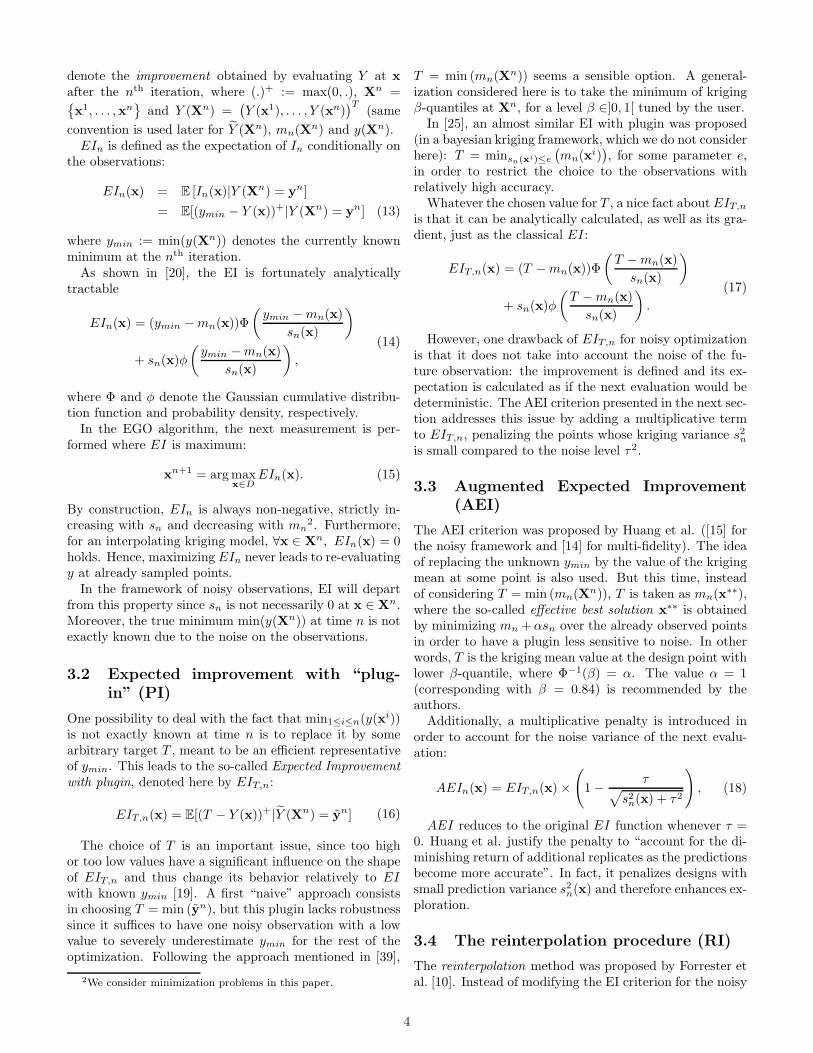
Contrarily to the noiseless case, mn(.) is not interpo-lating noisy measurements and s2n(.) does not vanish atthat points. Figure 1 shows an example of Kriging basedon noisy observations. Therewith, the model presentedin the paper slightly differs from the so-called kriging withnugget effect of the geostatistics literature [24, 6], where τ2

also appears in the covariance vector kn(x) (when x = xi),which makes it a discontinuous, interpolating model.

0 0.2 0.4 0.6 0.8 1−1

−0.5

0

0.5

1

1.5

2

2.5

3

Figure 1: Actual function (bold gray), Kriging mean (boldblack) and 90% confidence intervals (mixed line); the cir-cles are the observation values yi, the bars show the noiseamplitude (±2τ).

2.3 Covariance functions

A large variety of covariance kernels are available in theliterature (see , e. g., [33] or [28] for a detailed summary).The choice of the kernel and the value of its parametersdetermine the shape (smoothness, amplitude of the pre-diction variance, ...) of the kriging model. In this work,two kernels are considered:

• the Gaussian anisotropic kernel:

k(x,x′) = σ2 exp

−

d∑

j=1

(xj − x′jθj

)2 (7)

• the Matern tensor-product kernel with ν = 3/2:

k(x,x′) = σ2

1 +

√3

d∑

j=1

∣∣xj − x′j∣∣

θj

× exp

−

d∑

j=1

∣∣xj − x′j∣∣

θj

(8)

with x = [x1 . . . xd]. Both kernels depend on a set ofparameters, σ2 and {θ1, . . . , θd}, which are often referredto respectively as process variance and ranges.

2.4 Covariance parameter estimation

Covariance parameters are usually estimated based on theobservation vector yn. To accomplish this, several meth-ods are available, e. g., maximum-likelihood approaches,variogram estimation, or cross-validation. Here, we focuson maximum-likelihood estimation (MLE): σ2 and the θi’sare estimated by maximizing the probability density of yn

seen as a function of the covariance parameters, under aGaussian assumption on Yn:

L = (2π)−n

2 det[Kn

]− 1

2

exp

(−1

2(yn − µn1n)

TK−1

n (yn − µn1n)

)(9)

or equivalently by minimizing a negative multiple of thelog-likelihood (omitting constants):

l = log(det[Kn

])+ (yn − µn1n)

TK−1

n (yn − µn1n)

(10)In the noiseless case, there exists an explicit expression

for the optimal σ2 as a function of the θi, which allowsthe problem to be simplified to the optimization of theθi (”concentrated” or ”profile” log-likelihood). Unfortu-nately, the superimposed noise variance τ2 prevents usfrom doing so here, so the optimization of equation 10needs to be performed with respect to the whole vector ofparameters:

[σ2, θ1, . . . , θn] = argmin l(σ2, θ1, . . . , θn) (11)

where the dependency of l on the parameters appearsthrough Kn and µn. If τ

2 is unknown, it can also be con-sidered as a variable in the likelihood maximization. Here,we set it to the known variance of the superimposed ho-moscedastic noise according to the idea of benchmarkingthe approaches under ideal conditions.

3 Infill criteria

In the sequential procedure of most kriging-based optimiz-ers, the design point to be evaluated next is determinedbased on the optimization of a so-called infill criterion.This infill criterion uses information of the current meta-model in order to assess the utility of evaluating any can-didate design on the actual problem. In this section, wepresent the definitions of and the ideas behind the infillcriteria analyzed in our benchmark.

3.1 The classical (noiseless) Expected Im-provement

The Expected Improvement (EI) has probably become themost popular infill sampling criterion for kriging-basedglobal optimization of expensive-to-evaluate deterministicfunctions following the seminal paper of Jones et al. [20].Let

In(x) := (min(Y (Xn))− Y (x))+

(12)

3

denote the improvement obtained by evaluating Y at x

after the nth iteration, where (.)+ := max(0, .), Xn ={x1, . . . ,xn

}and Y (Xn) =

(Y (x1), . . . , Y (xn)

)T(same

convention is used later for Y (Xn), mn(Xn) and y(Xn).

EIn is defined as the expectation of In conditionally onthe observations:

EIn(x) = E [In(x)|Y (Xn) = yn]

= E[(ymin − Y (x))+|Y (Xn) = yn] (13)

where ymin := min(y(Xn)) denotes the currently knownminimum at the nth iteration.As shown in [20], the EI is fortunately analytically

tractable

EIn(x) = (ymin −mn(x))Φ

(ymin −mn(x)

sn(x)

)

+ sn(x)φ

(ymin −mn(x)

sn(x)

),

(14)

where Φ and φ denote the Gaussian cumulative distribu-tion function and probability density, respectively.In the EGO algorithm, the next measurement is per-

formed where EI is maximum:

xn+1 = argmaxx∈D

EIn(x). (15)

By construction, EIn is always non-negative, strictly in-creasing with sn and decreasing with mn

2. Furthermore,for an interpolating kriging model, ∀x ∈ Xn, EIn(x) = 0holds. Hence, maximizing EIn never leads to re-evaluatingy at already sampled points.In the framework of noisy observations, EI will depart

from this property since sn is not necessarily 0 at x ∈ Xn.Moreover, the true minimum min(y(Xn)) at time n is notexactly known due to the noise on the observations.

3.2 Expected improvement with “plug-in” (PI)

One possibility to deal with the fact that min1≤i≤n(y(xi))

is not exactly known at time n is to replace it by somearbitrary target T , meant to be an efficient representativeof ymin. This leads to the so-called Expected Improvement

with plugin, denoted here by EIT,n:

EIT,n(x) = E[(T − Y (x))+|Y (Xn) = yn] (16)

The choice of T is an important issue, since too highor too low values have a significant influence on the shapeof EIT,n and thus change its behavior relatively to EIwith known ymin [19]. A first “naive” approach consistsin choosing T = min (yn), but this plugin lacks robustnesssince it suffices to have one noisy observation with a lowvalue to severely underestimate ymin for the rest of theoptimization. Following the approach mentioned in [39],

2We consider minimization problems in this paper.

T = min (mn(Xn)) seems a sensible option. A general-

ization considered here is to take the minimum of krigingβ-quantiles at Xn, for a level β ∈]0, 1[ tuned by the user.In [25], an almost similar EI with plugin was proposed

(in a bayesian kriging framework, which we do not considerhere): T = minsn(xi)≤e

(mn(x

i)), for some parameter e,

in order to restrict the choice to the observations withrelatively high accuracy.Whatever the chosen value for T , a nice fact aboutEIT,n

is that it can be analytically calculated, as well as its gra-dient, just as the classical EI:

EIT,n(x) = (T −mn(x))Φ

(T −mn(x)

sn(x)

)

+ sn(x)φ

(T −mn(x)

sn(x)

).

(17)

However, one drawback of EIT,n for noisy optimizationis that it does not take into account the noise of the fu-ture observation: the improvement is defined and its ex-pectation is calculated as if the next evaluation would bedeterministic. The AEI criterion presented in the next sec-tion addresses this issue by adding a multiplicative termto EIT,n, penalizing the points whose kriging variance s2nis small compared to the noise level τ2.

3.3 Augmented Expected Improvement(AEI)

The AEI criterion was proposed by Huang et al. ([15] forthe noisy framework and [14] for multi-fidelity). The ideaof replacing the unknown ymin by the value of the krigingmean at some point is also used. But this time, insteadof considering T = min (mn(X

n)), T is taken as mn(x∗∗),

where the so-called effective best solution x∗∗ is obtainedby minimizing mn +αsn over the already observed pointsin order to have a plugin less sensitive to noise. In otherwords, T is the kriging mean value at the design point withlower β-quantile, where Φ−1(β) = α. The value α = 1(corresponding with β = 0.84) is recommended by theauthors.Additionally, a multiplicative penalty is introduced in

order to account for the noise variance of the next evalu-ation:

AEIn(x) = EIT,n(x)×(1− τ√

s2n(x) + τ2

), (18)

AEI reduces to the original EI function whenever τ =0. Huang et al. justify the penalty to “account for the di-minishing return of additional replicates as the predictionsbecome more accurate”. In fact, it penalizes designs withsmall prediction variance s2n(x) and therefore enhances ex-ploration.

3.4 The reinterpolation procedure (RI)

The reinterpolation method was proposed by Forrester etal. [10]. Instead of modifying the EI criterion for the noisy

4

case, the authors propose to use simultaneously a krigingwith noisy observations (as defined in equations 4 and 5)-called the regressing model- and an interpolating kriging,which is built as follows: The covariance structure and pa-rameters of the regressing model, as well as the design ofexperiments (DOE), are inherited, but the kriging meanpredictions of the regressing kriging at the DOE pointsare used as observation vector. Since this latter model isnoise-free, the classical EI can be used as an infill crite-rion. Summarizing, the reinterpolation procedure consistsof four steps:

1. Build a kriging based on the noisy observations yn

2. Compute the kriging predictor at the DOE pointsmn(x

1), . . . ,mn(xn)

3. Build an interpolating kriging model using Xn andyn = [mn(x

1), . . . ,mn(xn)]T

4. Solve x∗ = argmaxEIn(x) using the interpolatingmodel.

Note that this procedure was initially designed for “de-terministic” noise, due to numerical instabilities and ill-posedness of the simulated system. In that case, two veryclose designs would return different results, but repeat-ing the same experiment would return the same output.Hence, the reinterpolating procedure does not allow repe-titions since EI

(xi)= 0, 1 ≤ i ≤ n.

3.5 Expected Quantile Improvement(EQI)

The main idea behind the EQI criterion, as detailed in[26], is that in a noisy situation, the model predictormay be closer to the actual value than the original data;hence, an improvement should refer to the effect of a newobservation on the model. Taking the kriging quantileqn(x) = mn(x) + Φ−1(β)sn(x) (with β ∈ [0.5, 1[) as ameasure of reference, an improvement between steps n andn+ 1 is defined, similarly to the noiseless case, as:

In(x) :=

(min

1≤i≤n(Qn(x

i))−Qn+1(x)

)+

(19)

where Qn+1 is the quantile of the kriging updated witha new measurement at xn+1 = x. EQI is defined asE[In(x)|Y (Xn) = yn], the expectation being taken con-ditionally on the n current measurements and on the factthat a new measurement is made at xn+1, the new mea-surement Y (xn+1) being (at step n) a Gaussian randomvariable with mean mn(x

n+1) and variance s2n(xn+1) +

τ2n+1. It has been shown that the conditional distributionof Qn+1(x) is Gaussian and analytically derivable, whichleads to the following formula for the EQI:

EQIn(x) = (qmin −mQ(x))Φ

(qmin −mQ(x)

sQ(x)

)

+ sQ(x)φ

(qmin −mQ(x)

sQ(x)

),

(20)

where qmin := min1≤i≤n(qn(xi)) is the current best quan-

tile and mQ and sQ denote the mean and standard devia-tion of the future quantile Qn+1(x), respectively.In practice, mQ and sQ take the simple following form:

mQ(x) = mn(x) + Φ−1(β)

√τ2news

2n(x)

τ2new + s2n(x)(21)

s2Q(x) =

[s2n(x)

]2

τ2new + s2n(x)(22)

The future noise τ2new accounts for the limited optimiza-tion budget, and is set to τ2/(N − n), where N is themaximum number of observations. It is thus assumed thatthe remaining budget is completely spent for this solution,which is actually not desired. The above-defined rule canbe seen as a heuristic in order to slightly shift the focusof the optimization from exploration to exploitation alongthe iterations.

3.6 Approximate knowledge gradient(AKG)

The knowledge-gradient policy that has been proposed in[35] aims at measuring the global effect of a new mea-surement on the kriging mean. The knowledge improve-

ment is defined as the difference between the minima overD of the functions mn and mn+1. Since it requires twoglobal searches over D, no closed-form equation for con-tinuous optimization exists, but an efficient approximationhas been proposed, termed approximated knowledge gra-dient (AKG). The knowledge improvement is then definedas:

In(x) = min[Mn

(Xn+1

)]−min

[Mn+1

(Xn+1

)](23)

where Xn+1 = {Xn,x}, and Mn+1 denotes the mean ofthe kriging updated with a measurement at xn+1 = x.Note that Mn+1 = Qn+1 for β = 0.5, so conditionally forthe n first observations Mn+1 is a Gaussian process withknown distribution.In other words, an improvement is obtained if the mini-

mum of the new kriging mean is smaller that the minimumof the old kriging mean, both minima being taken over then+ 1 sample points. In contrast, EQI considers the min-imum of the old kriging quantile over the n past samplepoints, and the new kriging quantile at the new samplepoint only.AKG is defined as E[In(x)|Y (Xn) = yn;xn+1 = x].

The difficulty here lies in the computation of the condi-tional expectation of min

[Mn+1

(Xn+1

)], since it is the

minimum of a Gaussian vector. However, the problemcan be reformulated as

min[Mn+1

(Xn+1

)]= min

i∈{1,...,n+1}

[mn(x

i) + sM (xi)Z]

(24)where Z is standard normal (scalar), and:

sM (xi) =cn(x

i,x)√s2n(x) + τ2

(25)

5

with

cn(x,y) = k(x,y)− kn(y)TK−1

n kn(x)

+

(1− kn(y)K

−1n 1n

) (1− 1T

nK−1n kn(x)

)

1TnK

−1n 1n

(26)

Then, the expectation of the maximum takes the follow-ing form:

E

[minMn+1

(Xn+1

)|Y (Xn) = yn;xn+1 = x

]=

n∑

i=1

ai (Φ (ci+1)− Φ (ci)) + bi (φ (ci)− φ (ci+1)) (27)

where a, b and c are determined by running a small algo-rithm (see Table 1 in [35]).

3.7 Minimal quantile criteria (MQ)

The last method considered in this benchmark is perhapsthe most natural of the metamodel-based procedures andacts as a baseline for the other criteria. It consists of per-forming the next measurement where the current krigingmean or quantile is minimum:

xn+1 = argminx∈D

mn(x) + Φ(β)−1 × sn(x) (28)

This criterion can be found in [5] or [38]. In [38], Φ(β)−1 isan increasing function of the number of iterations in orderto ensure asymptotic convergence.Although recognized as less efficient compared to the

EI in the case of deterministic experiments [19], thismethod seems worth studying in this benchmark becauseit does not need any modification to handle noise. It alsohas shown successful applications in kriging-based multi-objective optimization [8, 27].

3.8 Integral criteria

Alternatively to pointwise-based criteria, two strategieshave been proposed that rely on global measures of im-provement: the Informational Approach to Global Opti-mization (IAGO) [40] and the Integrated Expected Con-ditional Improvement (IECI) [12]. The IAGO strategymaximizes the gain of information, i.e. selects for the nextevaluation the point that minimizes the expected condi-tional entropy of the minimizer; the IECI evaluates by howmuch a candidate measurement at a given point would af-fect the expected improvement over the design space. Bothstrategies can handle noise naturally. The major draw-back of such criteria is that they cannot be computed inclosed form and rely on numerical integration (contrarilyto the other criteria presented here, for which the value,and also the derivatives, can be calculated in an exactway, whatever the dimension). Comparing pointwise andintegral criteria brings up additional questions about thechoice of the integration method in moderate/high dimen-sion (which can become very expensive rapidly). For thosereasons, we did not include these two criteria into the cur-rent benchmark.

4 Design of the benchmark

4.1 Analytical test functions

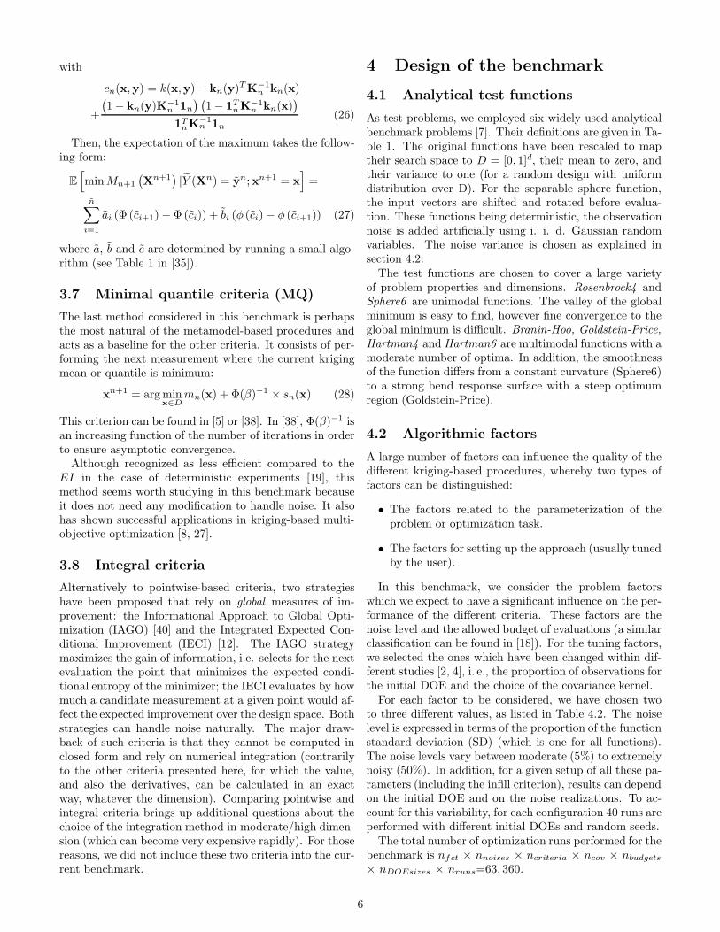
As test problems, we employed six widely used analyticalbenchmark problems [7]. Their definitions are given in Ta-ble 1. The original functions have been rescaled to maptheir search space to D = [0, 1]d, their mean to zero, andtheir variance to one (for a random design with uniformdistribution over D). For the separable sphere function,the input vectors are shifted and rotated before evalua-tion. These functions being deterministic, the observationnoise is added artificially using i. i. d. Gaussian randomvariables. The noise variance is chosen as explained insection 4.2.The test functions are chosen to cover a large variety

of problem properties and dimensions. Rosenbrock4 andSphere6 are unimodal functions. The valley of the globalminimum is easy to find, however fine convergence to theglobal minimum is difficult. Branin-Hoo, Goldstein-Price,Hartman4 and Hartman6 are multimodal functions with amoderate number of optima. In addition, the smoothnessof the function differs from a constant curvature (Sphere6)to a strong bend response surface with a steep optimumregion (Goldstein-Price).

4.2 Algorithmic factors

A large number of factors can influence the quality of thedifferent kriging-based procedures, whereby two types offactors can be distinguished:

• The factors related to the parameterization of theproblem or optimization task.

• The factors for setting up the approach (usually tunedby the user).

In this benchmark, we consider the problem factorswhich we expect to have a significant influence on the per-formance of the different criteria. These factors are thenoise level and the allowed budget of evaluations (a similarclassification can be found in [18]). For the tuning factors,we selected the ones which have been changed within dif-ferent studies [2, 4], i. e., the proportion of observations forthe initial DOE and the choice of the covariance kernel.For each factor to be considered, we have chosen two

to three different values, as listed in Table 4.2. The noiselevel is expressed in terms of the proportion of the functionstandard deviation (SD) (which is one for all functions).The noise levels vary between moderate (5%) to extremelynoisy (50%). In addition, for a given setup of all these pa-rameters (including the infill criterion), results can dependon the initial DOE and on the noise realizations. To ac-count for this variability, for each configuration 40 runs areperformed with different initial DOEs and random seeds.The total number of optimization runs performed for the

benchmark is nfct × nnoises × ncriteria × ncov × nbudgets

× nDOEsizes × nruns=63, 360.

6

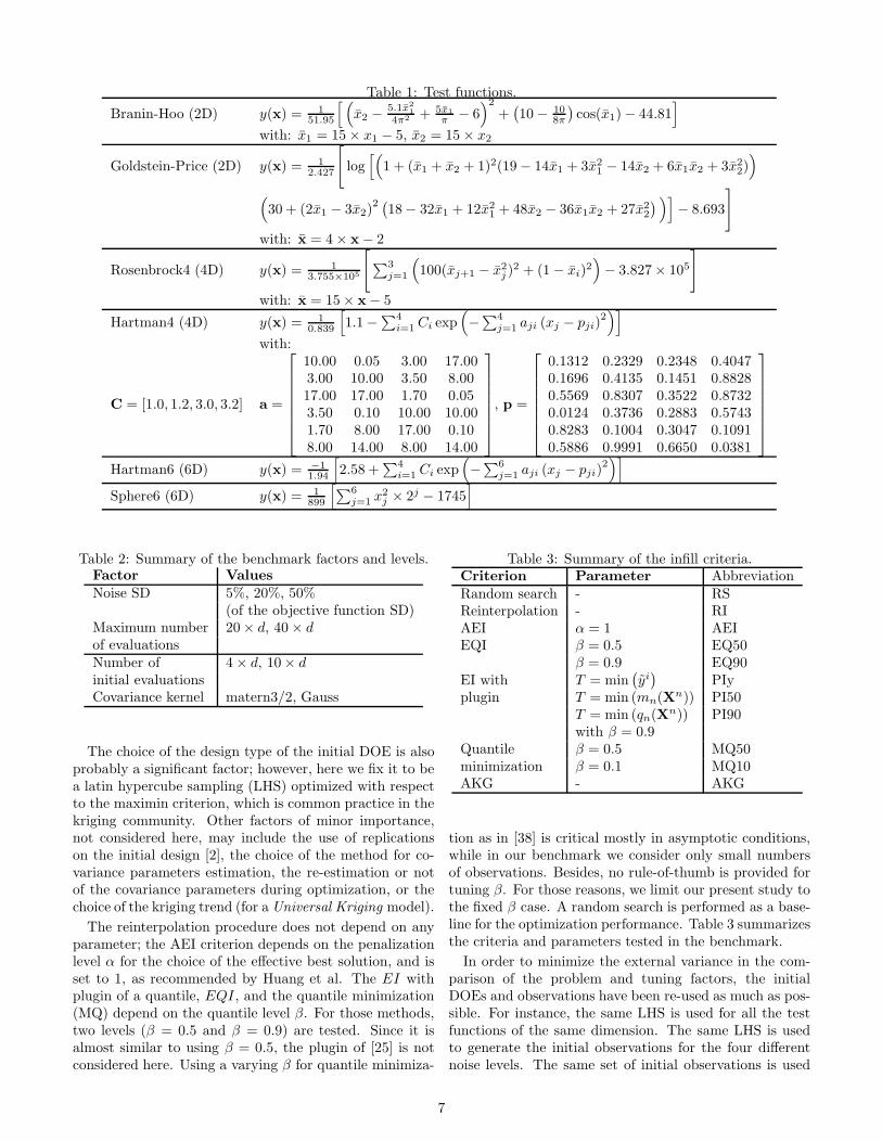
Table 1: Test functions.

Branin-Hoo (2D) y(x) = 151.95

[ (x2 − 5.1x2

1

4π2 + 5x1

π− 6)2

+(10− 10

8π

)cos(x1)− 44.81

]

with: x1 = 15× x1 − 5, x2 = 15× x2

Goldstein-Price (2D) y(x) = 12.427

[log[(

1 + (x1 + x2 + 1)2(19− 14x1 + 3x21 − 14x2 + 6x1x2 + 3x22))

(30 + (2x1 − 3x2)

2 (18− 32x1 + 12x21 + 48x2 − 36x1x2 + 27x22

) )]− 8.693

]

with: x = 4× x− 2

Rosenbrock4 (4D) y(x) = 13.755×105

[∑3

j=1

(100(xj+1 − x2j )

2 + (1− xi)2)− 3.827× 105

]

with: x = 15× x− 5

Hartman4 (4D) y(x) = 10.839

[1.1−∑4

i=1 Ci exp(−∑4

j=1 aji (xj − pji)2)]

with:

C = [1.0, 1.2, 3.0, 3.2] a =

10.00 0.05 3.00 17.003.00 10.00 3.50 8.0017.00 17.00 1.70 0.053.50 0.10 10.00 10.001.70 8.00 17.00 0.108.00 14.00 8.00 14.00

, p =

0.1312 0.2329 0.2348 0.40470.1696 0.4135 0.1451 0.88280.5569 0.8307 0.3522 0.87320.0124 0.3736 0.2883 0.57430.8283 0.1004 0.3047 0.10910.5886 0.9991 0.6650 0.0381

Hartman6 (6D) y(x) = −11.94

[2.58 +

∑4i=1 Ci exp

(−∑6

j=1 aji (xj − pji)2)]

Sphere6 (6D) y(x) = 1899

[∑6j=1 x

2j × 2j − 1745

]

Table 2: Summary of the benchmark factors and levels.Factor Values

Noise SD 5%, 20%, 50%(of the objective function SD)

Maximum number 20× d, 40× dof evaluationsNumber of 4× d, 10× dinitial evaluationsCovariance kernel matern3/2, Gauss

The choice of the design type of the initial DOE is alsoprobably a significant factor; however, here we fix it to bea latin hypercube sampling (LHS) optimized with respectto the maximin criterion, which is common practice in thekriging community. Other factors of minor importance,not considered here, may include the use of replicationson the initial design [2], the choice of the method for co-variance parameters estimation, the re-estimation or notof the covariance parameters during optimization, or thechoice of the kriging trend (for aUniversal Kriging model).

The reinterpolation procedure does not depend on anyparameter; the AEI criterion depends on the penalizationlevel α for the choice of the effective best solution, and isset to 1, as recommended by Huang et al. The EI withplugin of a quantile, EQI, and the quantile minimization(MQ) depend on the quantile level β. For those methods,two levels (β = 0.5 and β = 0.9) are tested. Since it isalmost similar to using β = 0.5, the plugin of [25] is notconsidered here. Using a varying β for quantile minimiza-

Table 3: Summary of the infill criteria.Criterion Parameter AbbreviationRandom search - RSReinterpolation - RIAEI α = 1 AEIEQI β = 0.5 EQ50

β = 0.9 EQ90EI with T = min

(yi)

PIyplugin T = min (mn(X

n)) PI50T = min (qn(X

n)) PI90with β = 0.9

Quantile β = 0.5 MQ50minimization β = 0.1 MQ10AKG - AKG

tion as in [38] is critical mostly in asymptotic conditions,while in our benchmark we consider only small numbersof observations. Besides, no rule-of-thumb is provided fortuning β. For those reasons, we limit our present study tothe fixed β case. A random search is performed as a base-line for the optimization performance. Table 3 summarizesthe criteria and parameters tested in the benchmark.

In order to minimize the external variance in the com-parison of the problem and tuning factors, the initialDOEs and observations have been re-used as much as pos-sible. For instance, the same LHS is used for all the testfunctions of the same dimension. The same LHS is usedto generate the initial observations for the four differentnoise levels. The same set of initial observations is used

7

for all the infill criteria.

4.3 Implementation issues and solutions

4.3.1 Optimization of the kriging parameters

In all kriging-based procedures, providing accurate covari-ance parameters is a crucial point. In particular, the rangeparameters (θj in eqs. 7 and 8) reflect the predicted activ-ity (or smoothness) of the objective function, which havea great effect on the shape of the infill criteria.The parameter estimation is here done by maximum

likelihood, as defined in section 2.4, using the R packageDiceKriging [29]. Since the likelihood is known to oftenhave local maxima for values corresponding to either verysmall range (white noise) or very large range (constantresponse), the covariance parameters are bounded to sen-sible intervals. These intervals have been found by per-forming pre-experiments on the chosen test functions andare wide enough to cover the requirements of the differentcriteria.Since Rosenbrock4 and Sphere6 have a very low activity,

the covariance bounds for the range parameters are cho-sen as [0.5, 5], which allows to have a very smooth krigingmodel. For Branin-Hoo, Goldstein-Price, Hartman4 andHartman6, the range bounds are set to [0.1, 1], which al-lows to model high activity responses.In our setup, the parameters are estimated first using

the initial DOE, and re-estimated after each additionalmeasurement. The old parameters are included as poten-tial candidates for the likelihood optimization, so the newparameters cannot be worse (in terms of likelihood) thanthe old ones. Nevertheless, it has been found that forsome criteria, the parameter re-estimation may fail due tonumerical instability in the inversion of the covariance ma-trix. When this occurs, the model is updated based the oldcovariance parameters. In particular, the reinterpolationtechnique is sensitive to these problems since it uses aninterpolating kriging on smoothed data. In case of failure,a small nugget is added to the interpolating model (in or-der to ease the covariance matrix inversion). If the modelcomputation is still not possible, the run is terminated andthe results for the last feasible iteration are used.

4.3.2 Optimization of the infill criteria

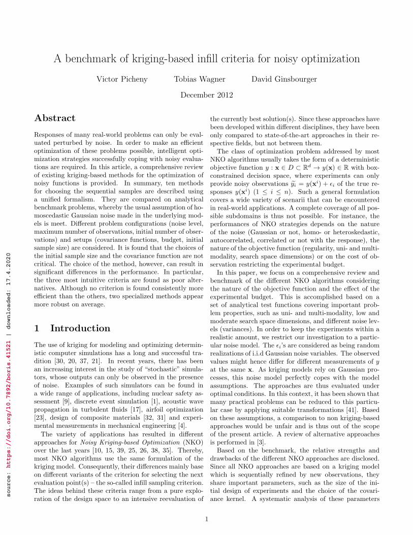
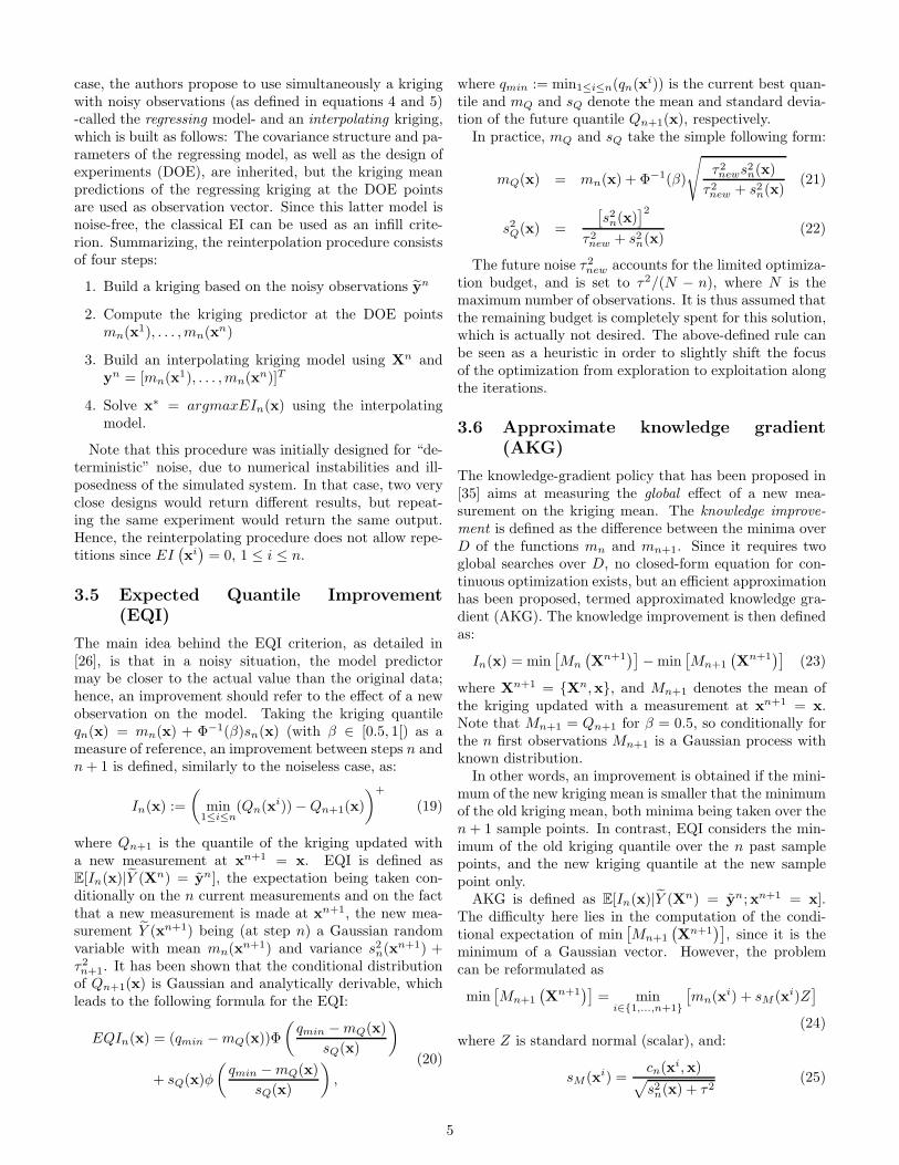
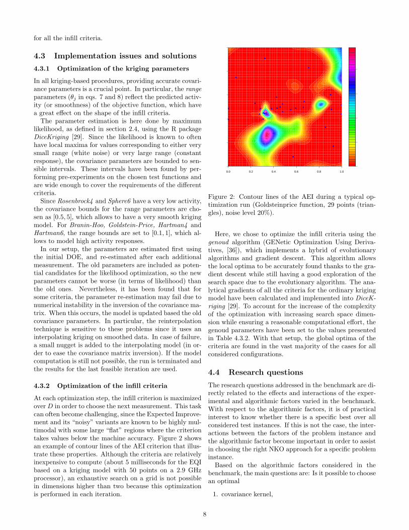
At each optimization step, the infill criterion is maximizedoverD in order to choose the next measurement. This taskcan often become challenging, since the Expected Improve-ment and its “noisy” variants are known to be highly mul-timodal with some large “flat” regions where the criteriontakes values below the machine accuracy. Figure 2 showsan example of contour lines of the AEI criterion that illus-trate these properties. Although the criteria are relativelyinexpensive to compute (about 5 milliseconds for the EQIbased on a kriging model with 50 points on a 2.9 GHzprocessor), an exhaustive search on a grid is not possiblein dimensions higher than two because this optimizationis performed in each iteration.

0.0000

0.0005

0.0010

0.0015

0.0020

0.0 0.2 0.4 0.6 0.8 1.0

0.0

0.2

0.4

0.6

0.8

1.0

Figure 2: Contour lines of the AEI during a typical op-timization run (Goldsteinprice function, 29 points (trian-gles), noise level 20%).

Here, we chose to optimize the infill criteria using thegenoud algorithm (GENetic Optimization Using Deriva-tives, [36]), which implements a hybrid of evolutionaryalgorithms and gradient descent. This algorithm allowsthe local optima to be accurately found thanks to the gra-dient descent while still having a good exploration of thesearch space due to the evolutionary algorithm. The ana-lytical gradients of all the criteria for the ordinary krigingmodel have been calculated and implemented into DiceK-

riging [29]. To account for the increase of the complexityof the optimization with increasing search space dimen-sion while ensuring a reasonable computational effort, thegenoud parameters have been set to the values presentedin Table 4.3.2. With that setup, the global optima of thecriteria are found in the vast majority of the cases for allconsidered configurations.

4.4 Research questions

The research questions addressed in the benchmark are di-rectly related to the effects and interactions of the exper-imental and algorithmic factors varied in the benchmark.With respect to the algorithmic factors, it is of practicalinterest to know whether there is a specific best over allconsidered test instances. If this is not the case, the inter-actions between the factors of the problem instance andthe algorithmic factor become important in order to assistin choosing the right NKO approach for a specific probleminstance.Based on the algorithmic factors considered in the

benchmark, the main questions are: Is it possible to choosean optimal

1. covariance kernel,

8

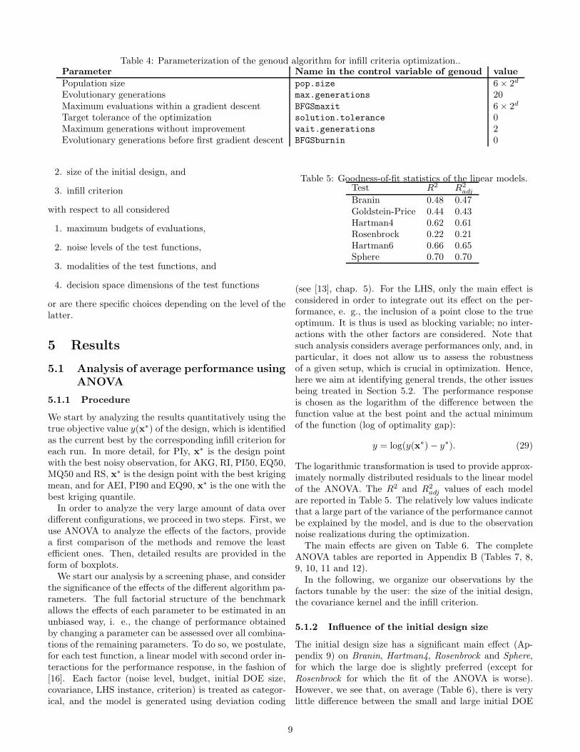
Table 4: Parameterization of the genoud algorithm for infill criteria optimization..Parameter Name in the control variable of genoud value

Population size pop.size 6× 2d

Evolutionary generations max.generations 20Maximum evaluations within a gradient descent BFGSmaxit 6× 2d

Target tolerance of the optimization solution.tolerance 0Maximum generations without improvement wait.generations 2Evolutionary generations before first gradient descent BFGSburnin 0

2. size of the initial design, and

3. infill criterion

with respect to all considered

1. maximum budgets of evaluations,

2. noise levels of the test functions,

3. modalities of the test functions, and

4. decision space dimensions of the test functions

or are there specific choices depending on the level of thelatter.

5 Results

5.1 Analysis of average performance usingANOVA

5.1.1 Procedure

We start by analyzing the results quantitatively using thetrue objective value y(x∗) of the design, which is identifiedas the current best by the corresponding infill criterion foreach run. In more detail, for PIy, x∗ is the design pointwith the best noisy observation, for AKG, RI, PI50, EQ50,MQ50 and RS, x∗ is the design point with the best krigingmean, and for AEI, PI90 and EQ90, x∗ is the one with thebest kriging quantile.In order to analyze the very large amount of data over

different configurations, we proceed in two steps. First, weuse ANOVA to analyze the effects of the factors, providea first comparison of the methods and remove the leastefficient ones. Then, detailed results are provided in theform of boxplots.We start our analysis by a screening phase, and consider

the significance of the effects of the different algorithm pa-rameters. The full factorial structure of the benchmarkallows the effects of each parameter to be estimated in anunbiased way, i. e., the change of performance obtainedby changing a parameter can be assessed over all combina-tions of the remaining parameters. To do so, we postulate,for each test function, a linear model with second order in-teractions for the performance response, in the fashion of[16]. Each factor (noise level, budget, initial DOE size,covariance, LHS instance, criterion) is treated as categor-ical, and the model is generated using deviation coding

Table 5: Goodness-of-fit statistics of the linear models.Test R2 R2

adj

Branin 0.48 0.47Goldstein-Price 0.44 0.43Hartman4 0.62 0.61Rosenbrock 0.22 0.21Hartman6 0.66 0.65Sphere 0.70 0.70

(see [13], chap. 5). For the LHS, only the main effect isconsidered in order to integrate out its effect on the per-formance, e. g., the inclusion of a point close to the trueoptimum. It is thus is used as blocking variable; no inter-actions with the other factors are considered. Note thatsuch analysis considers average performances only, and, inparticular, it does not allow us to assess the robustnessof a given setup, which is crucial in optimization. Hence,here we aim at identifying general trends, the other issuesbeing treated in Section 5.2. The performance responseis chosen as the logarithm of the difference between thefunction value at the best point and the actual minimumof the function (log of optimality gap):

y = log(y(x∗)− y∗). (29)

The logarithmic transformation is used to provide approx-imately normally distributed residuals to the linear modelof the ANOVA. The R2 and R2

adj values of each modelare reported in Table 5. The relatively low values indicatethat a large part of the variance of the performance cannotbe explained by the model, and is due to the observationnoise realizations during the optimization.The main effects are given on Table 6. The complete

ANOVA tables are reported in Appendix B (Tables 7, 8,9, 10, 11 and 12).In the following, we organize our observations by the

factors tunable by the user: the size of the initial design,the covariance kernel and the infill criterion.

5.1.2 Influence of the initial design size

The initial design size has a significant main effect (Ap-pendix 9) on Branin, Hartman4, Rosenbrock and Sphere,for which the large doe is slightly preferred (except forRosenbrock for which the fit of the ANOVA is worse).However, we see that, on average (Table 6), there is verylittle difference between the small and large initial DOE

9

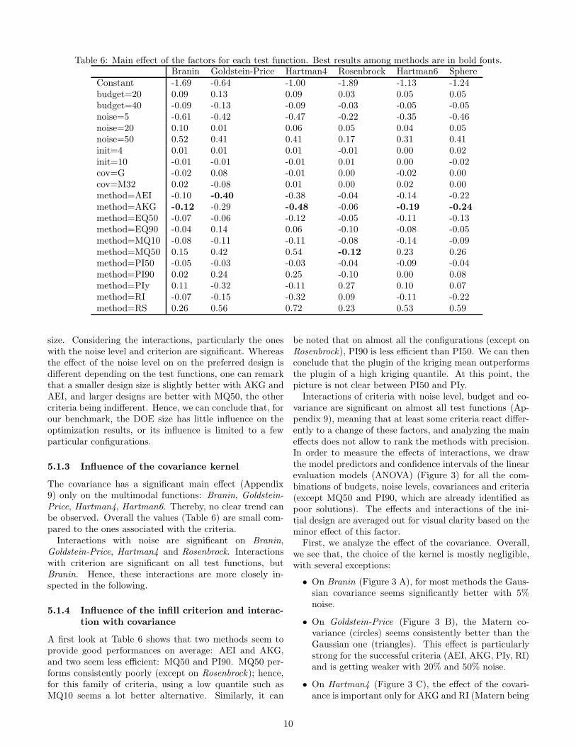
Table 6: Main effect of the factors for each test function. Best results among methods are in bold fonts.Branin Goldstein-Price Hartman4 Rosenbrock Hartman6 Sphere

Constant -1.69 -0.64 -1.00 -1.89 -1.13 -1.24budget=20 0.09 0.13 0.09 0.03 0.05 0.05budget=40 -0.09 -0.13 -0.09 -0.03 -0.05 -0.05noise=5 -0.61 -0.42 -0.47 -0.22 -0.35 -0.46noise=20 0.10 0.01 0.06 0.05 0.04 0.05noise=50 0.52 0.41 0.41 0.17 0.31 0.41init=4 0.01 0.01 0.01 -0.01 0.00 0.02init=10 -0.01 -0.01 -0.01 0.01 0.00 -0.02cov=G -0.02 0.08 -0.01 0.00 -0.02 0.00cov=M32 0.02 -0.08 0.01 0.00 0.02 0.00method=AEI -0.10 -0.40 -0.38 -0.04 -0.14 -0.22method=AKG -0.12 -0.29 -0.48 -0.06 -0.19 -0.24

method=EQ50 -0.07 -0.06 -0.12 -0.05 -0.11 -0.13method=EQ90 -0.04 0.14 0.06 -0.10 -0.08 -0.05method=MQ10 -0.08 -0.11 -0.11 -0.08 -0.14 -0.09method=MQ50 0.15 0.42 0.54 -0.12 0.23 0.26method=PI50 -0.05 -0.03 -0.03 -0.04 -0.09 -0.04method=PI90 0.02 0.24 0.25 -0.10 0.00 0.08method=PIy 0.11 -0.32 -0.11 0.27 0.10 0.07method=RI -0.07 -0.15 -0.32 0.09 -0.11 -0.22method=RS 0.26 0.56 0.72 0.23 0.53 0.59

size. Considering the interactions, particularly the oneswith the noise level and criterion are significant. Whereasthe effect of the noise level on on the preferred design isdifferent depending on the test functions, one can remarkthat a smaller design size is slightly better with AKG andAEI, and larger designs are better with MQ50, the othercriteria being indifferent. Hence, we can conclude that, forour benchmark, the DOE size has little influence on theoptimization results, or its influence is limited to a fewparticular configurations.

5.1.3 Influence of the covariance kernel

The covariance has a significant main effect (Appendix9) only on the multimodal functions: Branin, Goldstein-

Price, Hartman4, Hartman6. Thereby, no clear trend canbe observed. Overall the values (Table 6) are small com-pared to the ones associated with the criteria.Interactions with noise are significant on Branin,

Goldstein-Price, Hartman4 and Rosenbrock. Interactionswith criterion are significant on all test functions, butBranin. Hence, these interactions are more closely in-spected in the following.

5.1.4 Influence of the infill criterion and interac-

tion with covariance

A first look at Table 6 shows that two methods seem toprovide good performances on average: AEI and AKG,and two seem less efficient: MQ50 and PI90. MQ50 per-forms consistently poorly (except on Rosenbrock); hence,for this family of criteria, using a low quantile such asMQ10 seems a lot better alternative. Similarly, it can

be noted that on almost all the configurations (except onRosenbrock), PI90 is less efficient than PI50. We can thenconclude that the plugin of the kriging mean outperformsthe plugin of a high kriging quantile. At this point, thepicture is not clear between PI50 and PIy.Interactions of criteria with noise level, budget and co-

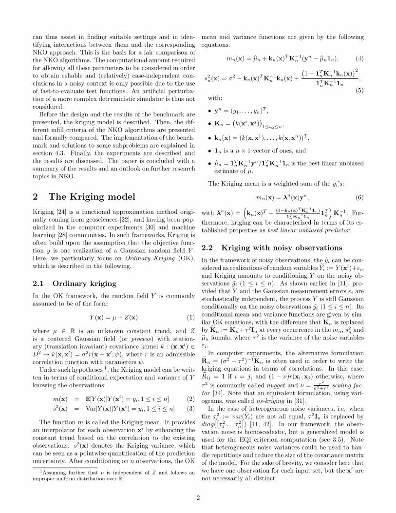
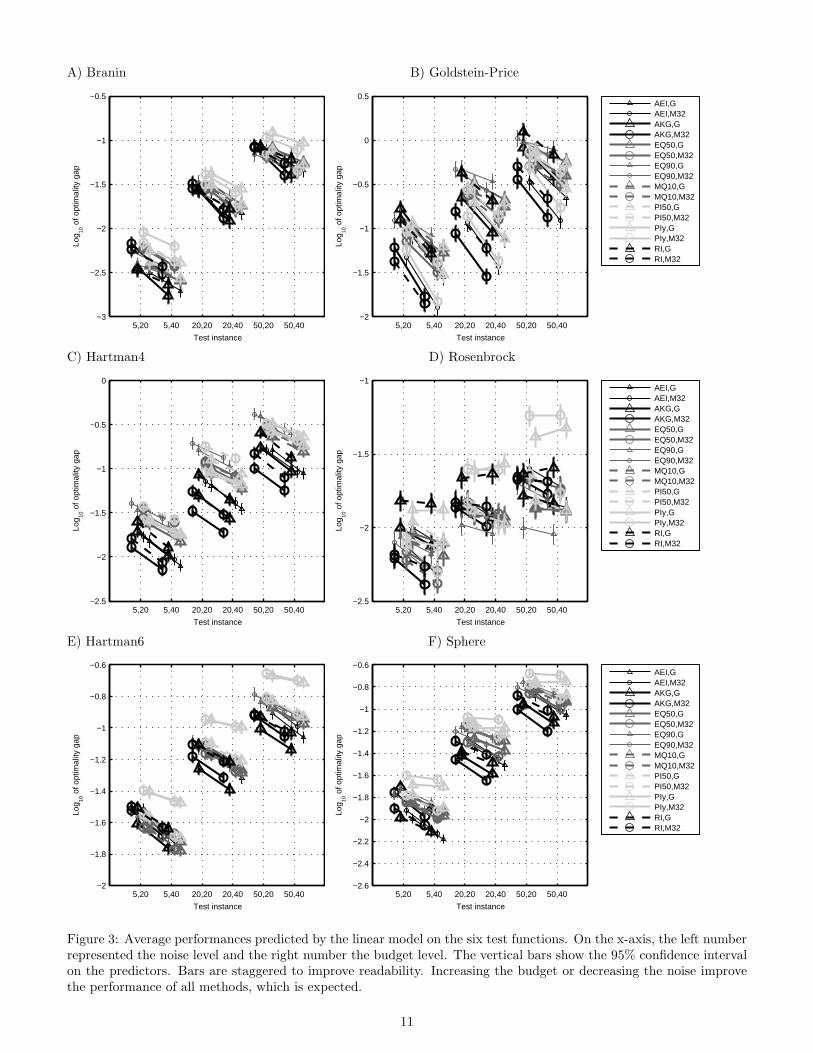
variance are significant on almost all test functions (Ap-pendix 9), meaning that at least some criteria react differ-ently to a change of these factors, and analyzing the maineffects does not allow to rank the methods with precision.In order to measure the effects of interactions, we drawthe model predictors and confidence intervals of the linearevaluation models (ANOVA) (Figure 3) for all the com-binations of budgets, noise levels, covariances and criteria(except MQ50 and PI90, which are already identified aspoor solutions). The effects and interactions of the ini-tial design are averaged out for visual clarity based on theminor effect of this factor.First, we analyze the effect of the covariance. Overall,

we see that, the choice of the kernel is mostly negligible,with several exceptions:

• On Branin (Figure 3 A), for most methods the Gaus-sian covariance seems significantly better with 5%noise.

• On Goldstein-Price (Figure 3 B), the Matern co-variance (circles) seems consistently better than theGaussian one (triangles). This effect is particularlystrong for the successful criteria (AEI, AKG, PIy, RI)and is getting weaker with 20% and 50% noise.

• On Hartman4 (Figure 3 C), the effect of the covari-ance is important only for AKG and RI (Matern being

10

A) Branin B) Goldstein-Price

5,20 5,40 20,20 20,40 50,20 50,40−3

−2.5

−2

−1.5

−1

−0.5

Test instance

Log 10

of o

ptim

ality

gap

5,20 5,40 20,20 20,40 50,20 50,40−2

−1.5

−1

−0.5

0

0.5

Test instanceLo

g 10 o

f opt

imal

ity g

ap

AEI,GAEI,M32AKG,GAKG,M32EQ50,GEQ50,M32EQ90,GEQ90,M32MQ10,GMQ10,M32PI50,GPI50,M32PIy,GPIy,M32RI,GRI,M32

C) Hartman4 D) Rosenbrock

5,20 5,40 20,20 20,40 50,20 50,40−2.5

−2

−1.5

−1

−0.5

0

Test instance

Log 10

of o

ptim

ality

gap

5,20 5,40 20,20 20,40 50,20 50,40−2.5

−2

−1.5

−1

Test instance

Log 10

of o

ptim

ality

gap

AEI,GAEI,M32AKG,GAKG,M32EQ50,GEQ50,M32EQ90,GEQ90,M32MQ10,GMQ10,M32PI50,GPI50,M32PIy,GPIy,M32RI,GRI,M32

E) Hartman6 F) Sphere

5,20 5,40 20,20 20,40 50,20 50,40−2

−1.8

−1.6

−1.4

−1.2

−1

−0.8

−0.6

Test instance

Log 10

of o

ptim

ality

gap

5,20 5,40 20,20 20,40 50,20 50,40−2.6

−2.4

−2.2

−2

−1.8

−1.6

−1.4

−1.2

−1

−0.8

−0.6

Test instance

Log 10

of o

ptim

ality

gap

AEI,GAEI,M32AKG,GAKG,M32EQ50,GEQ50,M32EQ90,GEQ90,M32MQ10,GMQ10,M32PI50,GPI50,M32PIy,GPIy,M32RI,GRI,M32

Figure 3: Average performances predicted by the linear model on the six test functions. On the x-axis, the left numberrepresented the noise level and the right number the budget level. The vertical bars show the 95% confidence intervalon the predictors. Bars are staggered to improve readability. Increasing the budget or decreasing the noise improvethe performance of all methods, which is expected.

11

slightly better) and PI50 and MQ10, where Gauss issuperior.

• On Hartman6 (Figure 3 E), the Matern covariance isslightly better for AKG with 20% and 50% noise.

• On Sphere (Figure 3 F), the Gauss covariance isslightly better for AKG with 20% and 50% noise.

Ranking between the methods is configuration depen-dent, and no method clearly appears as best here. How-ever, we can observe that:

• AKG, AEI, RI and PIy form a group of more effi-cient methods on Goldstein-Price, especially with theMatern covariance.

• AKG is best on Hartman4, regardless of the budgetor noise level, and on Hartman6 and Sphere for the20% and 50% noise levels.

• EQ90 is best on Rosenbrock for the 20% and 50%noise levels.

Inversely, some methods are significantly less efficienton some configurations:

• EQ90 and PI50 work poorly on Goldstein-Price withhigh noise and on Hartman4.

• With Gaussian covariance, RI works poorly on Rosen-

brock.

• PIy is the worst method on Branin, Rosenbrock, Hart-

man6 and Sphere, regardless of the configuration.

Interaction between method and budget is limited toa few configurations. Indeed, the slope between budgets20 and 40 is almost independent of the noise level and themethod, except for the worst and best methods. The effectis particularly strong on Rosenbrock, where the slope evenbecomes positive for PIy and RI, implying that a higherbudget results in a worse solution. Inversely, on Goldstein-

Price, it appears clearly that the best methods tend tomake a better use of the additional budget.

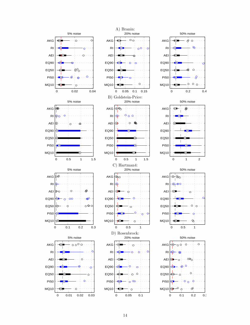
5.2 Detailed analysis of infill criteria us-ing boxplots

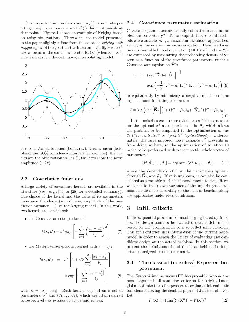
In this section, we propose a detailed comparison of themethods. Based on the previous observations, we limitnow our analysis to the following criteria: AKG, RI, AEI,EQ50, EQ90, PI50 and MQ10. The performance measureis the absolute difference between the function value at thebest point (y(x∗) and the actual minimum of the function(y∗) rescaled by the function standard deviation (σy , herealways equal to one):

D =|y(x∗)− y∗|

σy(30)

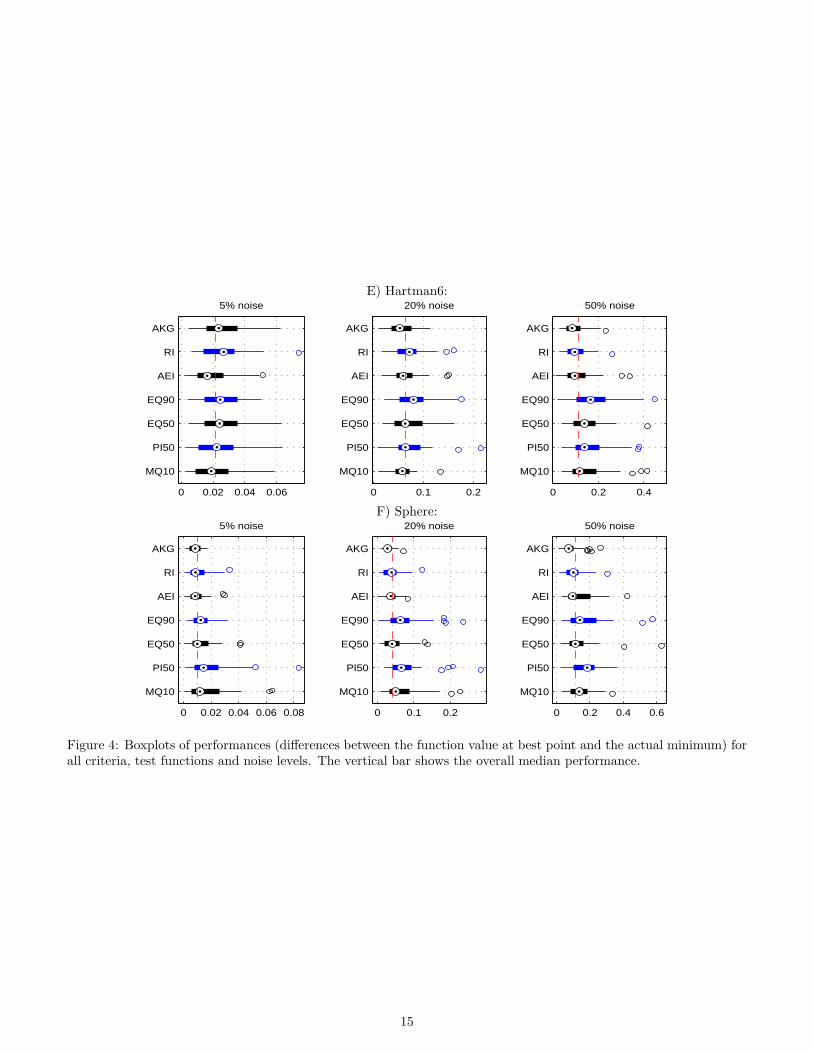
We represent the results in the form of boxplots for eachmethod, test function and noise level. To limit the amount

of figures, we show the results for the high budget only,since from Figure 3 it can be seen that the contrasts areslightly higher. We show the results with the Matern co-variance and the small initial DOE, which have been foundto have little influence of the results, but which providesuperior numerical stability and have a small beneficialinteraction with the appropriate methods.

On Branin (A), with 5% noise, all the criteria accu-rately identify one of the minima, which is expected sincethis function is very easy to optimize. With 20% noise, allthe median performances are very good, although someoutliers can be observed. With 50% noise, all the crite-ria fail at identifying one of the minima with precision,although with such a high noise the performances can beconsidered as quite satisfactory. While AKG and AEI wereidentified as slightly better than the other criteria by thelinear model (Table 6) on this function, no differences aremeasurable by the boxplots in the high noise case. In par-ticular, the performance of AEI improves with increasingnoise.

On Goldstein-Price (B), with 5% noise, we see that allthe median performances but MQ10 and PI50’s are verygood, but heavy tails can also be observed for EQ50 andEQ90. Indeed the basin of the global minimum is rela-tively small and was not found for several runs. With 20%noise, the difference is clear between AKG, RI and AEI,which almost always capture the global minimum, and theother criteria, which capture it approximately 25% of thetime. With 50% noise, results show a high variability, al-though the criteria identified as best by the linear model(Table 6 and Figure 3 B) perform globally better than theothers (AKG and AEI). For this function, the more ex-ploratory criteria are clearly superior, which is expectedsince the function is multimodal and the optimal region isnarrow. One may notice that this effect is much strongerthan on the main effect table, as only the results for theMatern covariance are considered.

On Hartman4 (C), again with 5% noise all the medianresults are very close to the actual optimum, but onlyAKG and RI do not have outliers. MQ10 and PI50 per-form worst in terms of upper quartile. With 20% and 50%noise, AKG, AEI and RI are globally better than the othermethods, and EQ90 and PI50 are slightly worse, whichconfirms the main effect values.

On Rosenbrock (D), differences are difficult to distin-guish, as expected from the main effect table. For allmethods, the optimum region is identified for more than75% of the runs for all noise levels. Note that the betterperformance of EQI detected on Figure 3 D) does not ap-pear, as the results with the Gaussian covariance are notused here.

On Hartman6 (E), only PIy appears as a poor alter-native. The medians are relatively close to the optimumvalue for all noise levels. With 50% noise, several runsfailed at providing a good solution. The global better per-formance of AKG, indicated by the linear model, is visiblein this graph, but also AEI and RI provide satisfactory

12

results.On Sphere (F), with 5% noise only PI50 and MQ10 are

slightly worse than the other methods. With 20% noise,EQ90, PI50 and MQ10 show larger variation. With 50%noise, AKG and RI are slightly better than the other meth-ods with respect to robustness as measured by their upperquartile.

6 Discussion

The first conclusion of this benchmark analysis is the lim-ited influence of the initial design size on the optimizationresults compared to other parameters. Using smaller ini-tial DOEs results in more optimization steps, which seemsintuitively more efficient. However, using larger initialDOEs ensures a good initial exploration, which reducesthe risk of converging to a local optimum, and tends toproduce more accurate models. These effects seem to bal-ance out each other regarding the optimization efficiency.For the user, this choice is thus not a critical one, re-gardless of the budget, noise, function modality or spacedimension.Another parameter of limited influence is the choice of

the covariance kernel, which is surprising since the twokernels considered here imply very different assumptionson the shape of the objective function (C1 for Matern3/2, C∞ for Gauss). Here it seems to be non-critical,except for one specific function (Goldstein-Price). Signif-icant interactions appear only with criteria, but tend tobe configuration-dependent (e.g., the better performanceof EQI and Gauss on Rosenbrock. The strongest influenceis detected with RI, as the reinterpolation step tends tolack robustness with Gauss, particularly on the smoothfunctions. In general, Matern may be preferred, as it mayprovide a better numerical stability for smooth functionsand allows a better detection of narrow optimal regions.The third parameter to be set up by the user is the infill

criterion. We found that no criterion outperforms the oth-ers on all configurations. However, out of the 10 criteriatested here, three can be considered as poor alternatives:PI90, PIy andMQ50. The criterionMQ50 was proposedessentially because it is relatively common practice in sur-rogate modeling to sequentially sampling at the minimumof the best predictor. Although known as a bad solutionfor deterministic functions [19], the question was left openin the noisy case. It is found that theMQ50 performancesare also poor in presence of noise so this solution is notcompetitive with other criteria.The poor performances of PI90 and PIy can be ex-

plained by looking at the EI equation 17. For PI90, byplugin a high quantile for T , the quantity T −mn is likelyto be positive and large: we indeed replace ymin by a tar-get that is very easy to reach, which makes the existingpoints look more interesting that they actually are andhinders exploration.With PIy, we also use a biased estimate (min(y)) of

ymin. With high noise in particular, ymin is likely to be

strongly underestimated, which results in increased explo-ration. Forcing exploration seems beneficial on Goldstein-Price, for which the minimum is indeed in a small valley,but for most of the configurations it was found inefficient.Note that similar results may be obtained with a low quan-tile plugin, PI10 for instance. Overall the criterion PI50(with an unbiased plugin) appears as a better alternative.This becomes particularly obvious on Rosenbrock wherethe predicted performance of PIy deteriorates with largerbudget, which can be caused by an increased probabilityof observing an extreme positively biased outlier withinmore iterations.

The RI and EQ90 criteria show contrasted perfor-mances depending on the configurations. By construction,the RI criterion is quite exploratory (in particular, it doesnot allow replications), which can be beneficial for opti-mization and eases the covariance parameter estimationstep (at least for the smoothed model), which explains thevery good performances in some cases. However, one canobserve that the RI performances decrease with higherbudget and higher noise. This can be imputed to the sub-sequent reinterpolation step, which may lack robustness inthose cases.

The relatively disappointing performances of EQ90(with regard to its complexity) can be explained by thefact that it is designed to return a solution with smallerror, which may favor repetitions or clustering instead ofexploration, and this benefit is not apparent in an analysisbased on the actual response values only. An illustrationof this characteristic is proposed in Appendix A.

The criteria MQ10, EQ50, AEI and AKG proved inour context to be competitive; the differences betweenthem depending on the configurations, although no par-ticular pattern regarding the problem parameters (noise,budget, dimension or modality) could be identified by thelinear model or the boxplots. The most contrasted resultswere obtained on Goldstein-Price with low and moderatenoise, in favor of the most exploratory criteria, as the op-timal region is narrow and difficult to detect.

On average, the AEI criterion seems a good option forour benchmark, since it is several times the best method,and is rarely very bad. As discussed, the plugin of the krig-ing mean, also used in AEI, is a sensible option, and theexploration enhancement due to the penalization function(see equation 18) seems also beneficial.

The AKG criterion provided the best performances onseveral configurations, and is also a sensible choice on av-erage. Two relatively poor performances with small noise(on Goldstein-Price and Sphere) might indicate that it ismore efficient with large noise. Indeed, contrarily to PI50,RI, EQ90 or AEI, AKG does not reduce to the classicalEI in absence of noise.

Overall, one important practical result of this bench-mark is that on many configurations, seven of the differentmethods provide relatively similar results. Hence, if AEIand AKG are identified as slightly better, another choicecan be made based on the user preference, in order to

13

A) Branin:

0 0.02 0.04

MQ10

PI50

EQ50

EQ90

AEI

RI

AKG

5% noise

0 0.05 0.1 0.15

MQ10

PI50

EQ50

EQ90

AEI

RI

AKG

20% noise

0 0.2 0.4

MQ10

PI50

EQ50

EQ90

AEI

RI

AKG

50% noise

B) Goldstein-Price:

0 0.5 1 1.5

MQ10

PI50

EQ50

EQ90

AEI

RI

AKG

5% noise

0 0.5 1 1.5

MQ10

PI50

EQ50

EQ90

AEI

RI

AKG

20% noise

0 1 2

MQ10

PI50

EQ50

EQ90

AEI

RI

AKG

50% noise

C) Hartman4:

0 0.1 0.2 0.3

MQ10

PI50

EQ50

EQ90

AEI

RI

AKG

5% noise

0 0.5 1

MQ10

PI50

EQ50

EQ90

AEI

RI

AKG

20% noise

0 0.5 1

MQ10

PI50

EQ50

EQ90

AEI

RI

AKG

50% noise

D) Rosenbrock:

0 0.01 0.02 0.03

MQ10

PI50

EQ50

EQ90

AEI

RI

AKG

5% noise

0 0.05 0.1

MQ10

PI50

EQ50

EQ90

AEI

RI

AKG

20% noise

0 0.1 0.2 0.3

MQ10

PI50

EQ50

EQ90

AEI

RI

AKG

50% noise

14

E) Hartman6:

0 0.02 0.04 0.06

MQ10

PI50

EQ50

EQ90

AEI

RI

AKG

5% noise

0 0.1 0.2

MQ10

PI50

EQ50

EQ90

AEI

RI

AKG

20% noise

0 0.2 0.4

MQ10

PI50

EQ50

EQ90

AEI

RI

AKG

50% noise

F) Sphere:

0 0.02 0.04 0.06 0.08

MQ10

PI50

EQ50

EQ90

AEI

RI

AKG

5% noise

0 0.1 0.2

MQ10

PI50

EQ50

EQ90

AEI

RI

AKG

20% noise

0 0.2 0.4 0.6

MQ10

PI50

EQ50

EQ90

AEI

RI

AKG

50% noise

Figure 4: Boxplots of performances (differences between the function value at best point and the actual minimum) forall criteria, test functions and noise levels. The vertical bar shows the overall median performance.

15

avoid replications (RI) or enhance uncertainty reduction(EQ90).For all methods, it seems that the results mainly depend

on the capability of kriging to fit the function based ona very small amount of information (small, noisy DOE).When it is the case (Hartman4, Hartman6, Sphere), allthe criteria lead to satisfying results, which means here,considering the difficulty of the optimization setup, an ap-proximate identification of the optimum region.It should be noted that the discussion proposed here

is specific to our framework (Gaussian, independent noisewith constant known variance), and might vary in a dif-ferent context. In particular, in the case of known het-eroscedastic noise, it is reasonable to conjecture that cri-teria that account for the noise amplitude (EQI, AKG)will have better performances than the other ones. In-versely, when little information is available for the noise,some criteria might prove to be more robust (RI, PI50,MQ10).

7 Conclusion

In this research, a comprehensive review of kriging-basedmethods for the optimization of noisy functions is pro-posed in a unified framework. The different methodsare compared in the case of independent, Gaussian, ho-moscedastic noise, based on a benchmark of analytical testfunctions with a large variety of setups that covers a widerange of potential applications. Variations on factors com-mon to all NKO procedures, such as the size of the initialset of experiments or the choice of the covariance kernel,are included in the analysis in order to assess their in-fluence as well as provide a comparison between methodsindependent of critical arbitrary choices. An extensive ex-perimental design and statistical tools are used to providea robust and unbiased performance analysis.First, we found that, apart from a small number of ex-

ceptions, the size of the initial DOE is not critical, whichmeans that the effect of having less sequential steps (withlarger initial DOE) is counterbalanced by the benefit ofa better initial exploration and surrogate model. Hence,the effect of this factor can be neglected without intro-ducing bias in future work. The covariance function isalso not a very important factor, which implies that, inthe noisy context, the exploration / exploitation trade-off sought for global optimization is achieved regardlessof this choice. The numerical stability of the approaches,however, can be often improved by avoiding the Gaussiankernel. In our benchmark, this particularly holds for theRI criterion. If some prior knowledge about the shapeof the response surface (smooth or rugged, uni- or multi-modal) exists, the kernel should be chosen accordingly, asshown on the Goldstein-Price function in our benchmark.Out of the criteria (and variants) detailed in this paper,

we found that several are either poor alternatives (PI90,MQ50) or lack robustness (PIy). The other criteria haverelatively similar performances, although, on average, the

augmented expected improvement (AEI) and the approx-imate knowledge gradient (AKG) were found as best al-ternatives. In our framework, the practical or statisticalconsiderations that motivated the multiplicity of the cri-teria seem dominated by the kriging modeling error dueto the very small amount of information available. Hence,the choice of the criterion may be based on user preference(to avoid replications, enhance uncertainty reduction, im-prove implementation robustness, etc.) without a criticaldeterioration of the performance.

Future research may address the evaluation of the NKOalgorithms performances for heteroscedastic noise scenarii,such as variance depending on input parameters (indepen-dently of the response), or noise linearly correlated withthe response, which are likely to be found in real wordproblems.

Acknowledgements

The contributions of Tobias Wagner to this paper arebased on investigations of the project D5 of the Col-laborative Research Center SFB/TR TRR 30, which iskindly supported by the Deutsche Forschungsgemeinschaft(DFG).

8 Appendix A: sample results for

four infill criteria

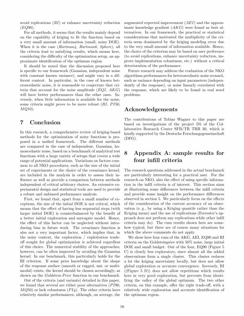
The research questions addressed in the actual benchmarkare particularly interesting for a practical user. For theresearch on NKO, also the effect of using specific informa-tion in the infill criteria is of interest. This section aimsat illustrating some differences between the infill criteriaand provide some insight on the performance differencesobserved in section 5. We particularly focus on the effectsof the consideration of the current accuracy of an obser-vation (e. g., by using a Kriging quantile rather than theKriging mean) and the use of replications (Forrester’s ap-proach does not perform any replications while other infillcriteria may do). The runs results shown here are some-how typical, but there are of course many situations forwhich the above comments do not apply.

We show here four runs of the AKG, AEI, EQ90 and RIcriteria on the Goldsteinprice with 50% noise, large initialDOE and small budget. Out of the four, EQ90 (Figure 5C) is clearly less exploratory, since almost all the addedobservations form a single cluster. This cluster reducesa lot the kriging uncertainty locally, but does not allowglobal exploration or accurate convergence. Inversely, RI((Figure 5 D)) does not allow repetitions which resultshere in very good exploration, but prevents from identi-fying the valley of the global optimum. The two othercriteria, on this example, offer the right trade-off, with arelatively wide exploration and accurate identification ofthe optimum region.

16

A) AKG B) AEI

−3

−2

−1

0

1

2

0.0 0.2 0.4 0.6 0.8 1.0

0.0

0.2

0.4

0.6

0.8

1.0

−3

−2

−1

0

1

2

0.0 0.2 0.4 0.6 0.8 1.0

0.0

0.2

0.4

0.6

0.8

1.0

C) EQ90 D) RI

−3

−2

−1

0

1

2

0.0 0.2 0.4 0.6 0.8 1.0

0.0

0.2

0.4

0.6

0.8

1.0

−3

−2

−1

0

1

2

0.0 0.2 0.4 0.6 0.8 1.0

0.0

0.2

0.4

0.6

0.8

1.0

Figure 5: Sample of optimization results obtained on the Goldsteinprice with 50% noise, large initial DOE and smallbudget. Initial observations are represented with filled triangles. The contour lines represent the actual function.

17

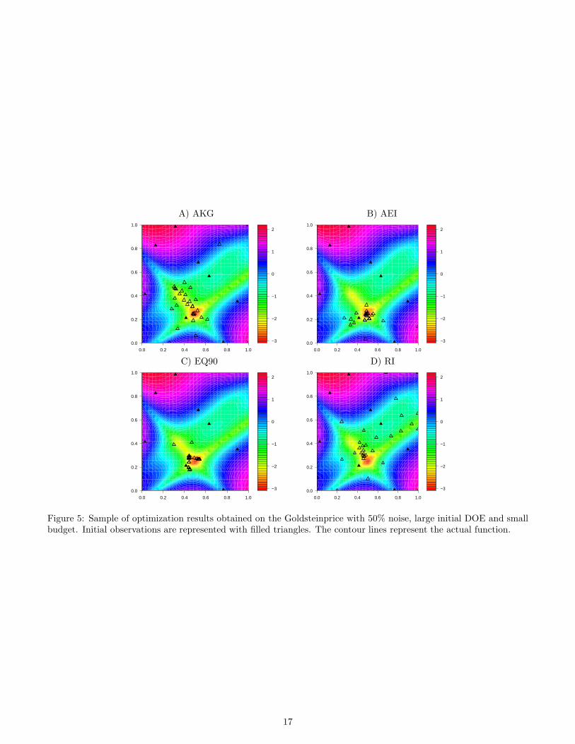
9 Appendix B: ANOVA tables ofthe linear models

Table 7: ANOVA table for the Branin test function.Source Sum Sq. d.f. F p-valbudget 89.6 1 308.79 **noise 2312.42 2 3984.63 **noise*budget 1.76 2 3.03 -init 1.41 1 4.87 *init*budget 0.23 1 0.8 -init*noise 8.56 2 14.75 **cov 4.99 1 17.19 **cov*budget 0.48 1 1.65 -cov*noise 32.82 2 56.55 **cov*init 0.94 1 3.25 -meth 143.31 10 49.39 **meth*budget 11.79 10 4.06 **meth*noise 78.19 20 13.47 **meth*init 13.64 10 4.7 **meth*cov 5.17 10 1.78 -lhs 62.92 39 5.56 **Error 3031.09 10446Total 5799.32 10559

Significance codes: 0 ‘**’ 0.01 ‘*’ 0.05 ‘-’ 1

Table 8: ANOVA table for the Goldstein-Price test func-tion.

Source Sum Sq. d.f. F p-valbudget 182.73 1 467.59 **noise 1194.92 2 1528.86 **noise*budget 7.33 2 9.38 **init 0.41 1 1.04 -init*budget 0.1 1 0.26 -init*noise 15.71 2 20.1 **cov 75.85 1 194.09 **cov*budget 6.39 1 16.35 **cov*noise 2.6 2 3.32 *cov*init 7.03 1 17.98 **meth 913.87 10 233.85 **meth*budget 53.03 10 13.57 **meth*noise 129.96 20 16.63 **meth*init 19.33 10 4.95 **meth*cov 64.51 10 16.51 **lhs 545.58 39 35.8 **Error 4082.16 10446Total 7301.5 10559

References

[1] Ankenman, B., Nelson, B.L., Staum, J.: Stochas-tic kriging for simulation metamodeling. OperationsResearch 58(2), 371–382 (2010). DOI 10.1287/opre.1090.0754

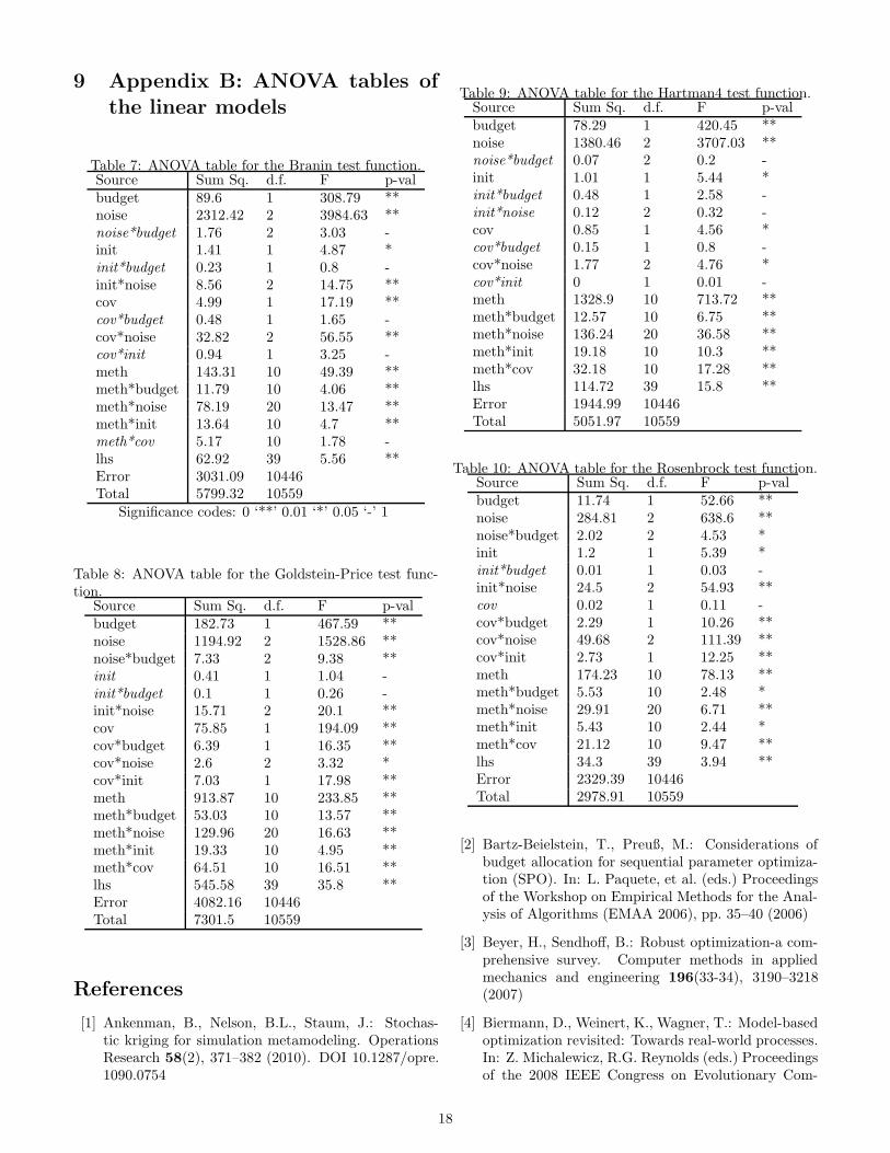
Table 9: ANOVA table for the Hartman4 test function.Source Sum Sq. d.f. F p-valbudget 78.29 1 420.45 **noise 1380.46 2 3707.03 **noise*budget 0.07 2 0.2 -init 1.01 1 5.44 *init*budget 0.48 1 2.58 -init*noise 0.12 2 0.32 -cov 0.85 1 4.56 *cov*budget 0.15 1 0.8 -cov*noise 1.77 2 4.76 *cov*init 0 1 0.01 -meth 1328.9 10 713.72 **meth*budget 12.57 10 6.75 **meth*noise 136.24 20 36.58 **meth*init 19.18 10 10.3 **meth*cov 32.18 10 17.28 **lhs 114.72 39 15.8 **Error 1944.99 10446Total 5051.97 10559

Table 10: ANOVA table for the Rosenbrock test function.Source Sum Sq. d.f. F p-valbudget 11.74 1 52.66 **noise 284.81 2 638.6 **noise*budget 2.02 2 4.53 *init 1.2 1 5.39 *init*budget 0.01 1 0.03 -init*noise 24.5 2 54.93 **cov 0.02 1 0.11 -cov*budget 2.29 1 10.26 **cov*noise 49.68 2 111.39 **cov*init 2.73 1 12.25 **meth 174.23 10 78.13 **meth*budget 5.53 10 2.48 *meth*noise 29.91 20 6.71 **meth*init 5.43 10 2.44 *meth*cov 21.12 10 9.47 **lhs 34.3 39 3.94 **Error 2329.39 10446Total 2978.91 10559

[2] Bartz-Beielstein, T., Preuß, M.: Considerations ofbudget allocation for sequential parameter optimiza-tion (SPO). In: L. Paquete, et al. (eds.) Proceedingsof the Workshop on Empirical Methods for the Anal-ysis of Algorithms (EMAA 2006), pp. 35–40 (2006)

[3] Beyer, H., Sendhoff, B.: Robust optimization-a com-prehensive survey. Computer methods in appliedmechanics and engineering 196(33-34), 3190–3218(2007)

[4] Biermann, D., Weinert, K., Wagner, T.: Model-basedoptimization revisited: Towards real-world processes.In: Z. Michalewicz, R.G. Reynolds (eds.) Proceedingsof the 2008 IEEE Congress on Evolutionary Com-

18

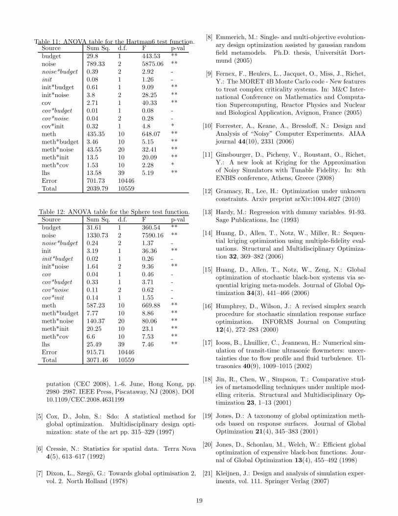
Table 11: ANOVA table for the Hartman6 test function.Source Sum Sq. d.f. F p-valbudget 29.8 1 443.53 **noise 789.33 2 5875.06 **noise*budget 0.39 2 2.92 -init 0.08 1 1.26 -init*budget 0.61 1 9.09 **init*noise 3.8 2 28.25 **cov 2.71 1 40.33 **cov*budget 0.01 1 0.08 -cov*noise 0.04 2 0.28 -cov*init 0.32 1 4.8 *meth 435.35 10 648.07 **meth*budget 3.46 10 5.15 **meth*noise 43.55 20 32.41 **meth*init 13.5 10 20.09 **meth*cov 1.53 10 2.28 *lhs 13.58 39 5.19 **Error 701.73 10446Total 2039.79 10559

Table 12: ANOVA table for the Sphere test function.Source Sum Sq. d.f. F p-valbudget 31.61 1 360.54 **noise 1330.73 2 7590.16 **noise*budget 0.24 2 1.37 -init 3.19 1 36.36 **init*budget 0.02 1 0.26 -init*noise 1.64 2 9.36 **cov 0.04 1 0.46 -cov*budget 0.33 1 3.71 -cov*noise 0.11 2 0.62 -cov*init 0.14 1 1.55 -meth 587.23 10 669.88 **meth*budget 7.77 10 8.86 **meth*noise 140.37 20 80.06 **meth*init 20.25 10 23.1 **meth*cov 6.6 10 7.53 **lhs 25.49 39 7.46 **Error 915.71 10446Total 3071.46 10559

putation (CEC 2008), 1.-6. June, Hong Kong, pp.2980–2987. IEEE Press, Piscataway, NJ (2008). DOI10.1109/CEC.2008.4631199

[5] Cox, D., John, S.: Sdo: A statistical method forglobal optimization. Multidisciplinary design opti-mization: state of the art pp. 315–329 (1997)

[6] Cressie, N.: Statistics for spatial data. Terra Nova4(5), 613–617 (1992)

[7] Dixon, L., Szego, G.: Towards global optimisation 2,vol. 2. North Holland (1978)

[8] Emmerich, M.: Single- and multi-objective evolution-ary design optimization assisted by gaussian randomfield metamodels. Ph.D. thesis, Universitat Dort-mund (2005)

[9] Fernex, F., Heulers, L., Jacquet, O., Miss, J., Richet,Y.: The MORET 4BMonte Carlo code - New featuresto treat complex criticality systems. In: M&C Inter-national Conference on Mathematics and Computa-tion Supercomputing, Reactor Physics and Nuclearand Biological Application, Avignon, France (2005)

[10] Forrester, A., Keane, A., Bressloff, N.: Design andAnalysis of “Noisy” Computer Experiments. AIAAjournal 44(10), 2331 (2006)

[11] Ginsbourger, D., Picheny, V., Roustant, O., Richet,Y.: A new look at Kriging for the Approximationof Noisy Simulators with Tunable Fidelity. In: 8thENBIS conference, Athens, Greece (2008)

[12] Gramacy, R., Lee, H.: Optimization under unknownconstraints. Arxiv preprint arXiv:1004.4027 (2010)

[13] Hardy, M.: Regression with dummy variables. 91-93.Sage Publications, Inc (1993)

[14] Huang, D., Allen, T., Notz, W., Miller, R.: Sequen-tial kriging optimization using multiple-fidelity eval-uations. Structural and Multidisciplinary Optimiza-tion 32, 369–382 (2006)

[15] Huang, D., Allen, T., Notz, W., Zeng, N.: Globaloptimization of stochastic black-box systems via se-quential kriging meta-models. Journal of Global Op-timization 34(3), 441–466 (2006)

[16] Humphrey, D., Wilson, J.: A revised simplex searchprocedure for stochastic simulation response surfaceoptimization. INFORMS Journal on Computing12(4), 272–283 (2000)

[17] Iooss, B., Lhuillier, C., Jeanneau, H.: Numerical sim-ulation of transit-time ultrasonic flowmeters: uncer-tainties due to flow profile and fluid turbulence. Ul-trasonics 40(9), 1009–1015 (2002)

[18] Jin, R., Chen, W., Simpson, T.: Comparative stud-ies of metamodelling techniques under multiple mod-elling criteria. Structural and Multidisciplinary Op-timization 23, 1–13 (2001)

[19] Jones, D.: A taxonomy of global optimization meth-ods based on response surfaces. Journal of GlobalOptimization 21(4), 345–383 (2001)

[20] Jones, D., Schonlau, M., Welch, W.: Efficient globaloptimization of expensive black-box functions. Jour-nal of Global Optimization 13(4), 455–492 (1998)

[21] Kleijnen, J.: Design and analysis of simulation exper-iments, vol. 111. Springer Verlag (2007)

19

[22] Krige, D.: A statistical approach to some basinc minevaluation problems on the witwatersrand. Journal ofthe South African Institute of Mining and Metallurgy52, 141 (1952)

[23] Li, W., Huyse, L., Padula, S.: Robust airfoil opti-mization to achieve drag reduction over a range ofmach numbers. Structural and Multidisciplinary Op-timization 24(1), 38–50 (2002)

[24] Matheron, G.: Le krigeage universel. Cahiers du cen-tre de morphologie mathematique 1 (1969)

[25] Osborne, M., Garnett, R., Roberts, S.: Gaussian pro-cesses for global optimization. In: 3rd InternationalConference on Learning and Intelligent Optimization(LION3), pp. 1–15 (2009)

[26] Picheny, V., Ginsbourger, D., Richet, Y.: Noisy ex-pected improvement and on-line computation time al-location for the optimization of simulators with tun-able fidelity. In: 2nd International Conference on En-gineering Optimization, September 6-9, 2010, Lisbon,Portugal (2010)

[27] Ponweiser, W., Wagner, T., Biermann, D., Vincze,M.: Multiobjective optimization on a limited amountof evaluations using model-assisted S-metric selec-tion. In: G. Rudolph, T. Jansen, S. Lucas, C. Poloni,N. Beume (eds.) Proceedings of the 10th Interna-tional Conference on Parallel Problem Solving fromNature (PPSN), 13.-17. September, Dortmund, no.5199 in Lecture Notes in Computer Science, pp. 784–794. Springer, Berlin (2008)

[28] Rasmussen, C., Williams, C.: Gaussian processes formachine learning. MIT Press (2006)

[29] Roustant, O., Ginsbourger, D., Deville, Y.: TheDiceKriging package: kriging-based metamodelingand optimization for computer experiments. Bookof abstract of the R User Conference (2009)

[30] Sacks, J., Welch, W., Mitchell, T., Wynn, H.: Designand analysis of computer experiments. Statistical sci-ence pp. 409–423 (1989)

[31] Sakata, S., Ashida, F.: Ns-kriging based microstruc-tural optimization applied to minimizing stochasticvariation of homogenized elasticity of fiber reinforcedcomposites. Structural and Multidisciplinary Opti-mization 38, 443–453 (2009)

[32] Sakata, S., Ashida, F., Zako, M.: Microstructural de-sign of composite materials using fixed-grid modelingand noise-resistant smoothed kriging-based approxi-mate optimization. Structural and MultidisciplinaryOptimization 36, 273–287 (2008)

[33] Santner, T., Williams, B., Notz, W.: The design andanalysis of computer experiments. Springer (2003)

[34] Sasena, M.: Flexibility and efficiency enhancementsfor constrained global design optimization with krig-ing approximations. Ph.D. thesis, University of Michi-gan (2002)

[35] Scott, W., Frazier, P., Powell, W.: The correlatedknowledge gradient for simulation optimization ofcontinuous parameters using gaussian process regres-sion. SIAM Journal on Optimization 21, 996 (2011)

[36] Sekhon, J., Mebane, W.: Genetic optimization usingderivatives. Political Analysis 7(1), 187 (1998)

[37] Simpson, T., Booker, A., Ghosh, D., Giunta, A.,Koch, P., Yang, R.J.: Approximation methods inmultidisciplinary analysis and optimization: a paneldiscussion. Structural and Multidisciplinary Opti-mization 27, 302–313 (2004)

[38] Srinivas, N., Krause, A., Kakade, S., Seeger, M.:Gaussian process optimization in the bandit setting:No regret and experimental design. In: 27th Interna-tional Conference on Machine Learning (ICML 2010)(2010)

[39] Vazquez, E., Villemonteix, J., Sidorkiewicz, M., Wal-ter, E.: Global optimization based on noisy eval-uations: an empirical study of two statistical ap-proaches. In: Journal of Physics: Conference Series,vol. 135, p. 012100 (2008)

[40] Villemonteix, J., Vazquez, E., Walter, E.: An in-formational approach to the global optimization ofexpensive-to-evaluate functions. Journal of GlobalOptimization 44(4), 509–534 (2009)

[41] Wagner, T., Wessing, S.: On the effect of responsetransformations in sequential parameter optimiza-tion. Evolutionary Computation 20(2), 229–248(2012). DOI 10.1162/EVCO a 00061

[42] Yin, J., Ng, S., Ng, K.: Kriging metamodel with mod-ified nugget-effect: The heteroscedastic variance case.Computers & Industrial Engineering 61(3), 760–777(2011)

20