Embed Size (px)
Citation preview
A Case Study on Fraud Detection
L. Torgo
Faculdade de Ciências / LIAAD-INESC TEC, LAUniversidade do Porto
Aug, 2017
Problem Description
Problem Description
The Context
Fraud detection is a key activity in many organizationsFrauds are associated with unusual activitiesThese activities can be seen as outliers from a data analysisperspective
The Concrete Application
Transaction reports of salesmen of a companySalesmen free to set the selling price of a series of productsFor each transaction salesmen report back the product, the soldquantity and the overall value of the transaction
© L.Torgo (FCUP - LIAAD / UP) Fraud Detection Aug, 2017 2 / 95
Problem Description The Data
The Available Data
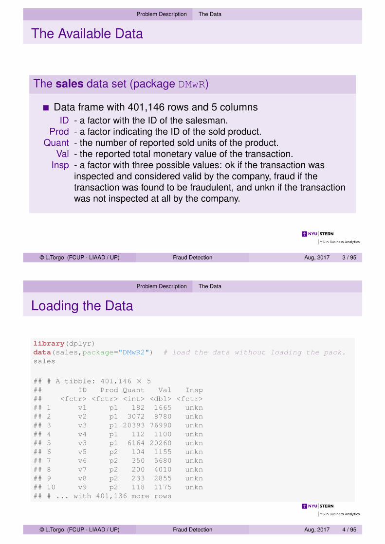
The sales data set (package DMwR)
Data frame with 401,146 rows and 5 columnsID - a factor with the ID of the salesman.
Prod - a factor indicating the ID of the sold product.Quant - the number of reported sold units of the product.
Val - the reported total monetary value of the transaction.Insp - a factor with three possible values: ok if the transaction was
inspected and considered valid by the company, fraud if thetransaction was found to be fraudulent, and unkn if the transactionwas not inspected at all by the company.
© L.Torgo (FCUP - LIAAD / UP) Fraud Detection Aug, 2017 3 / 95
Problem Description The Data
Loading the Data
library(dplyr)data(sales,package="DMwR2") # load the data without loading the pack.sales
## # A tibble: 401,146 × 5## ID Prod Quant Val Insp## <fctr> <fctr> <int> <dbl> <fctr>## 1 v1 p1 182 1665 unkn## 2 v2 p1 3072 8780 unkn## 3 v3 p1 20393 76990 unkn## 4 v4 p1 112 1100 unkn## 5 v3 p1 6164 20260 unkn## 6 v5 p2 104 1155 unkn## 7 v6 p2 350 5680 unkn## 8 v7 p2 200 4010 unkn## 9 v8 p2 233 2855 unkn## 10 v9 p2 118 1175 unkn## # ... with 401,136 more rows
© L.Torgo (FCUP - LIAAD / UP) Fraud Detection Aug, 2017 4 / 95
Exploratory Analysis
Main Data Statistics
summary(sales)
## ID Prod Quant Val## v431 : 10159 p1125 : 3923 Min. : 100 Min. : 1005## v54 : 6017 p3774 : 1824 1st Qu.: 107 1st Qu.: 1345## v426 : 3902 p1437 : 1720 Median : 168 Median : 2675## v1679 : 3016 p1917 : 1702 Mean : 8442 Mean : 14617## v1085 : 3001 p4089 : 1598 3rd Qu.: 738 3rd Qu.: 8680## v1183 : 2642 p2742 : 1519 Max. :473883883 Max. :4642955## (Other):372409 (Other):388860 NA's :13842 NA's :1182## Insp## ok : 14462## unkn :385414## fraud: 1270########
nrow(filter(sales,is.na(Quant), is.na(Val)))
## [1] 888
table(sales$Insp)/nrow(sales)*100
#### ok unkn fraud## 3.605171 96.078236 0.316593
© L.Torgo (FCUP - LIAAD / UP) Fraud Detection Aug, 2017 5 / 95
Exploratory Analysis
Unit Price
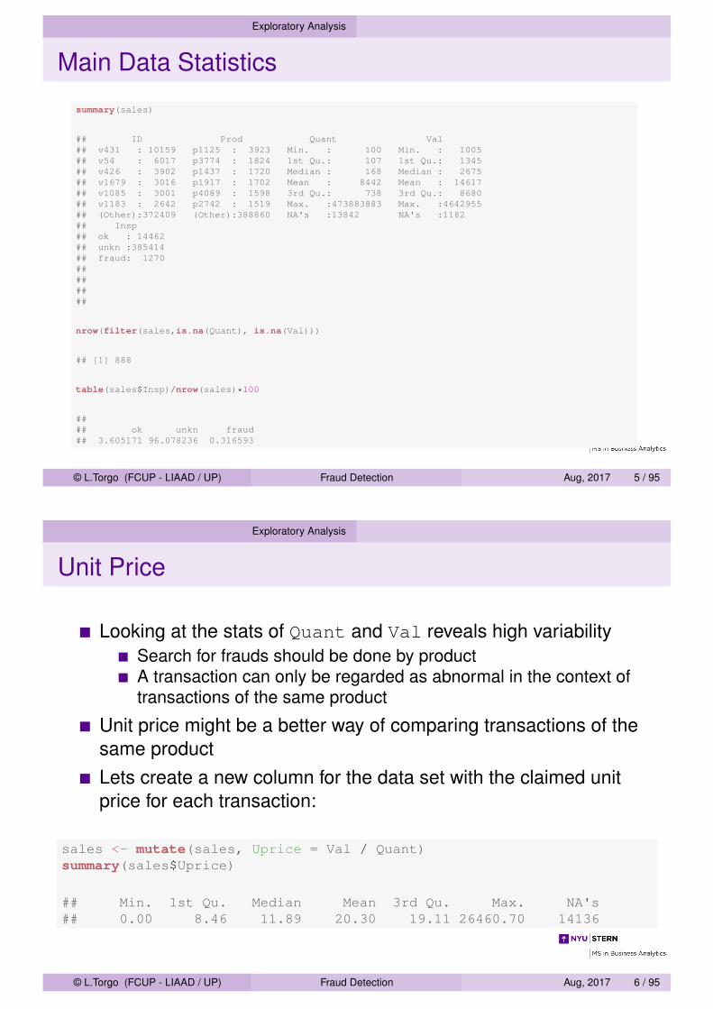
Looking at the stats of Quant and Val reveals high variabilitySearch for frauds should be done by productA transaction can only be regarded as abnormal in the context oftransactions of the same product
Unit price might be a better way of comparing transactions of thesame productLets create a new column for the data set with the claimed unitprice for each transaction:
sales <- mutate(sales, Uprice = Val / Quant)summary(sales$Uprice)
## Min. 1st Qu. Median Mean 3rd Qu. Max. NA's## 0.00 8.46 11.89 20.30 19.11 26460.70 14136
© L.Torgo (FCUP - LIAAD / UP) Fraud Detection Aug, 2017 6 / 95
Exploratory Analysis
Variability Among Salesmen and Products
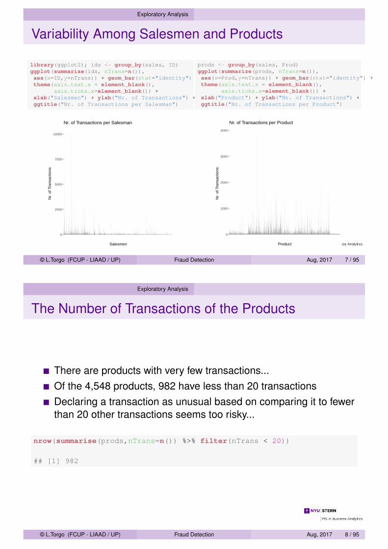
library(ggplot2); ids <- group_by(sales, ID)ggplot(summarize(ids, nTrans=n()),aes(x=ID,y=nTrans)) + geom_bar(stat="identity") +theme(axis.text.x = element_blank(),
axis.ticks.x=element_blank()) +xlab("Salesmen") + ylab("Nr. of Transactions") +ggtitle("Nr. of Transactions per Salesman")
0
2500
5000
7500
10000
Salesmen
Nr.
of T
rans
actio
ns
Nr. of Transactions per Salesman
prods <- group_by(sales, Prod)ggplot(summarize(prods, nTrans=n()),aes(x=Prod,y=nTrans)) + geom_bar(stat="identity") +theme(axis.text.x = element_blank(),
axis.ticks.x=element_blank()) +xlab("Product") + ylab("Nr. of Transactions") +ggtitle("Nr. of Transactions per Product")
0
1000
2000
3000
4000
Product
Nr.
of T
rans
actio
ns
Nr. of Transactions per Product
© L.Torgo (FCUP - LIAAD / UP) Fraud Detection Aug, 2017 7 / 95
Exploratory Analysis
The Number of Transactions of the Products
There are products with very few transactions...Of the 4,548 products, 982 have less than 20 transactionsDeclaring a transaction as unusual based on comparing it to fewerthan 20 other transactions seems too risky...
nrow(summarise(prods,nTrans=n()) %>% filter(nTrans < 20))
## [1] 982
© L.Torgo (FCUP - LIAAD / UP) Fraud Detection Aug, 2017 8 / 95
Exploratory Analysis
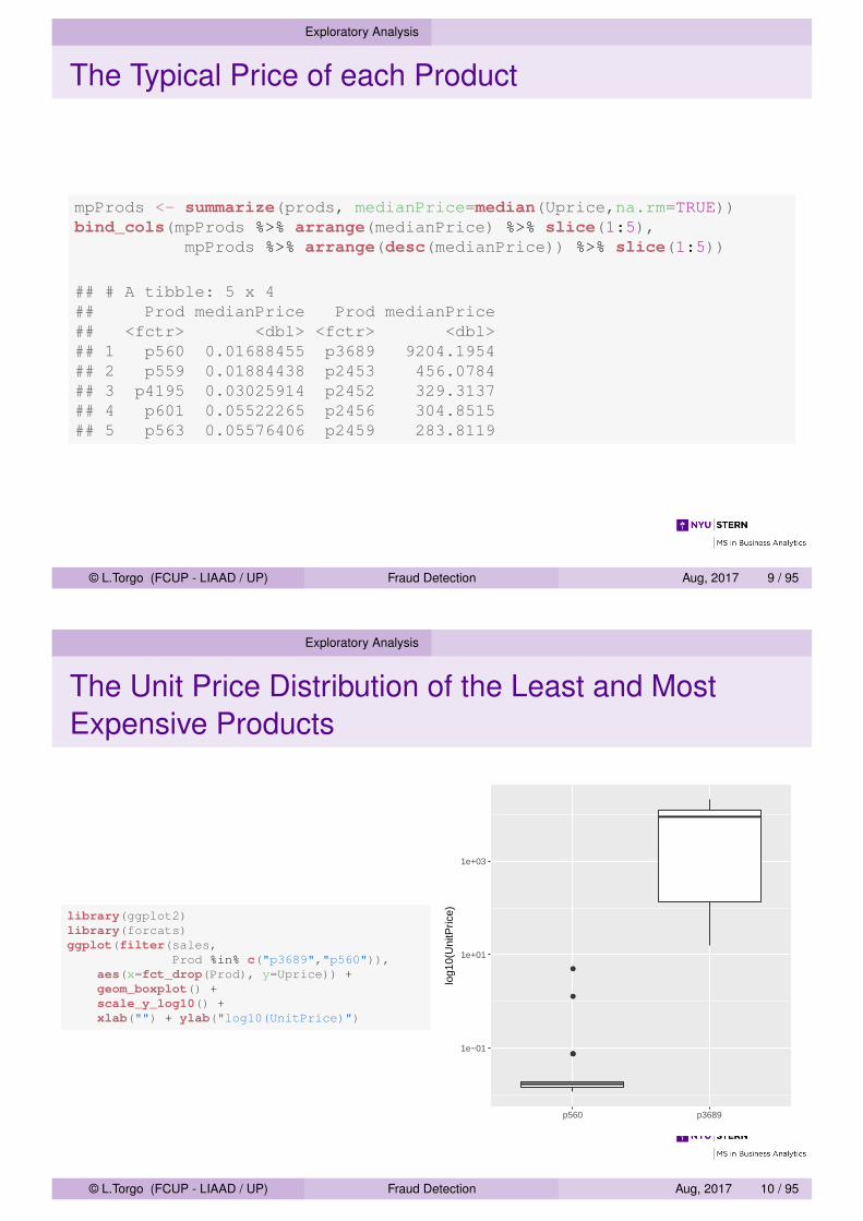
The Typical Price of each Product
mpProds <- summarize(prods, medianPrice=median(Uprice,na.rm=TRUE))bind_cols(mpProds %>% arrange(medianPrice) %>% slice(1:5),
mpProds %>% arrange(desc(medianPrice)) %>% slice(1:5))
## # A tibble: 5 x 4## Prod medianPrice Prod medianPrice## <fctr> <dbl> <fctr> <dbl>## 1 p560 0.01688455 p3689 9204.1954## 2 p559 0.01884438 p2453 456.0784## 3 p4195 0.03025914 p2452 329.3137## 4 p601 0.05522265 p2456 304.8515## 5 p563 0.05576406 p2459 283.8119
© L.Torgo (FCUP - LIAAD / UP) Fraud Detection Aug, 2017 9 / 95
Exploratory Analysis
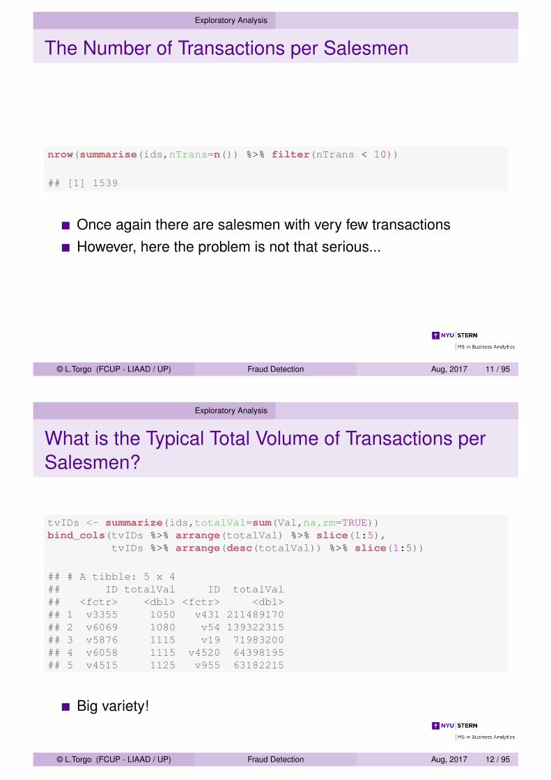
The Unit Price Distribution of the Least and MostExpensive Products
library(ggplot2)library(forcats)ggplot(filter(sales,
Prod %in% c("p3689","p560")),aes(x=fct_drop(Prod), y=Uprice)) +geom_boxplot() +scale_y_log10() +xlab("") + ylab("log10(UnitPrice)")
●
●
●
●
1e−01
1e+01
1e+03
p560 p3689
log1
0(U
nitP
rice)
© L.Torgo (FCUP - LIAAD / UP) Fraud Detection Aug, 2017 10 / 95
Exploratory Analysis
The Number of Transactions per Salesmen
nrow(summarise(ids,nTrans=n()) %>% filter(nTrans < 10))
## [1] 1539
Once again there are salesmen with very few transactionsHowever, here the problem is not that serious...
© L.Torgo (FCUP - LIAAD / UP) Fraud Detection Aug, 2017 11 / 95
Exploratory Analysis
What is the Typical Total Volume of Transactions perSalesmen?
tvIDs <- summarize(ids,totalVal=sum(Val,na.rm=TRUE))bind_cols(tvIDs %>% arrange(totalVal) %>% slice(1:5),
tvIDs %>% arrange(desc(totalVal)) %>% slice(1:5))
## # A tibble: 5 x 4## ID totalVal ID totalVal## <fctr> <dbl> <fctr> <dbl>## 1 v3355 1050 v431 211489170## 2 v6069 1080 v54 139322315## 3 v5876 1115 v19 71983200## 4 v6058 1115 v4520 64398195## 5 v4515 1125 v955 63182215
Big variety!
© L.Torgo (FCUP - LIAAD / UP) Fraud Detection Aug, 2017 12 / 95
Exploratory Analysis
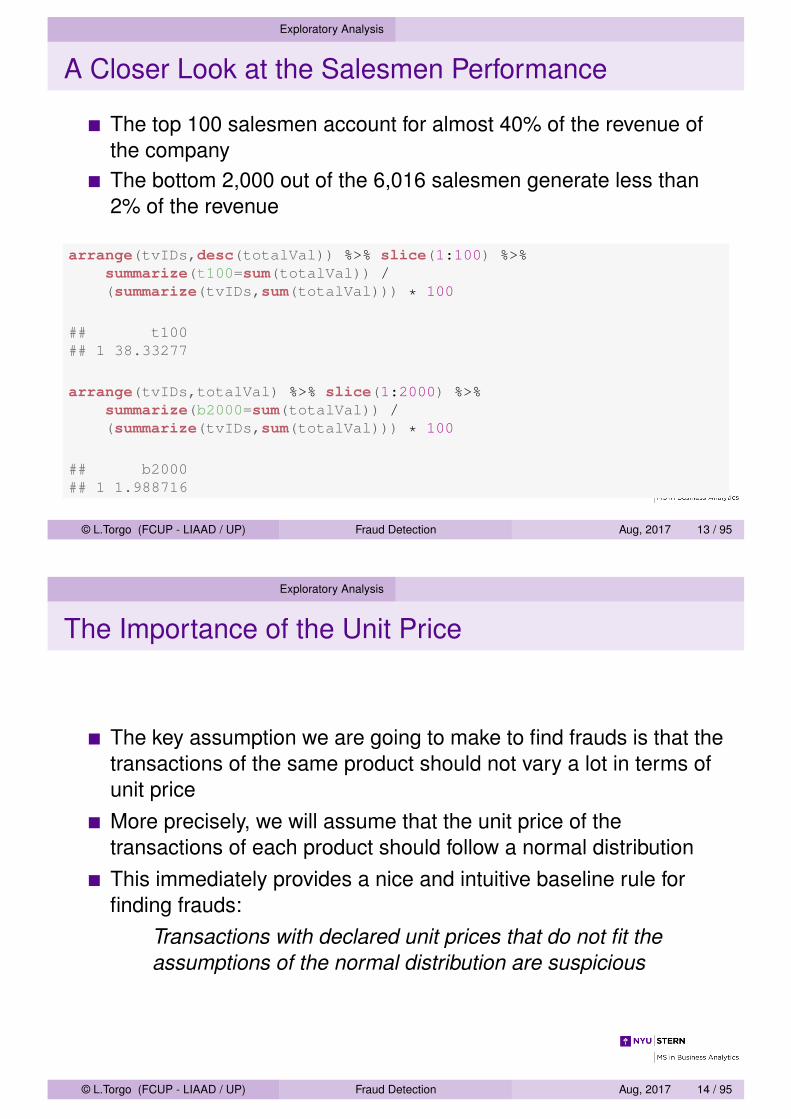
A Closer Look at the Salesmen Performance
The top 100 salesmen account for almost 40% of the revenue ofthe companyThe bottom 2,000 out of the 6,016 salesmen generate less than2% of the revenue
arrange(tvIDs,desc(totalVal)) %>% slice(1:100) %>%summarize(t100=sum(totalVal)) /(summarize(tvIDs,sum(totalVal))) * 100
## t100## 1 38.33277
arrange(tvIDs,totalVal) %>% slice(1:2000) %>%summarize(b2000=sum(totalVal)) /(summarize(tvIDs,sum(totalVal))) * 100
## b2000## 1 1.988716
© L.Torgo (FCUP - LIAAD / UP) Fraud Detection Aug, 2017 13 / 95
Exploratory Analysis
The Importance of the Unit Price
The key assumption we are going to make to find frauds is that thetransactions of the same product should not vary a lot in terms ofunit priceMore precisely, we will assume that the unit price of thetransactions of each product should follow a normal distributionThis immediately provides a nice and intuitive baseline rule forfinding frauds:
Transactions with declared unit prices that do not fit theassumptions of the normal distribution are suspicious
© L.Torgo (FCUP - LIAAD / UP) Fraud Detection Aug, 2017 14 / 95
Exploratory Analysis
The Importance of the Unit Price (2)
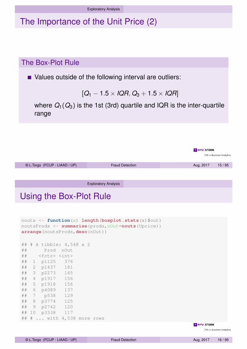
The Box-Plot Rule
Values outside of the following interval are outliers:
[Q1 − 1.5× IQR,Q3 + 1.5× IQR]
where Q1(Q3) is the 1st (3rd) quartile and IQR is the inter-quartilerange
© L.Torgo (FCUP - LIAAD / UP) Fraud Detection Aug, 2017 15 / 95
Exploratory Analysis
Using the Box-Plot Rule
nouts <- function(x) length(boxplot.stats(x)$out)noutsProds <- summarise(prods,nOut=nouts(Uprice))arrange(noutsProds,desc(nOut))
## # A tibble: 4,548 x 2## Prod nOut## <fctr> <int>## 1 p1125 376## 2 p1437 181## 3 p2273 165## 4 p1917 156## 5 p1918 156## 6 p4089 137## 7 p538 129## 8 p3774 125## 9 p2742 120## 10 p3338 117## # ... with 4,538 more rows
© L.Torgo (FCUP - LIAAD / UP) Fraud Detection Aug, 2017 16 / 95
Exploratory Analysis
Using the Box-Plot Rule
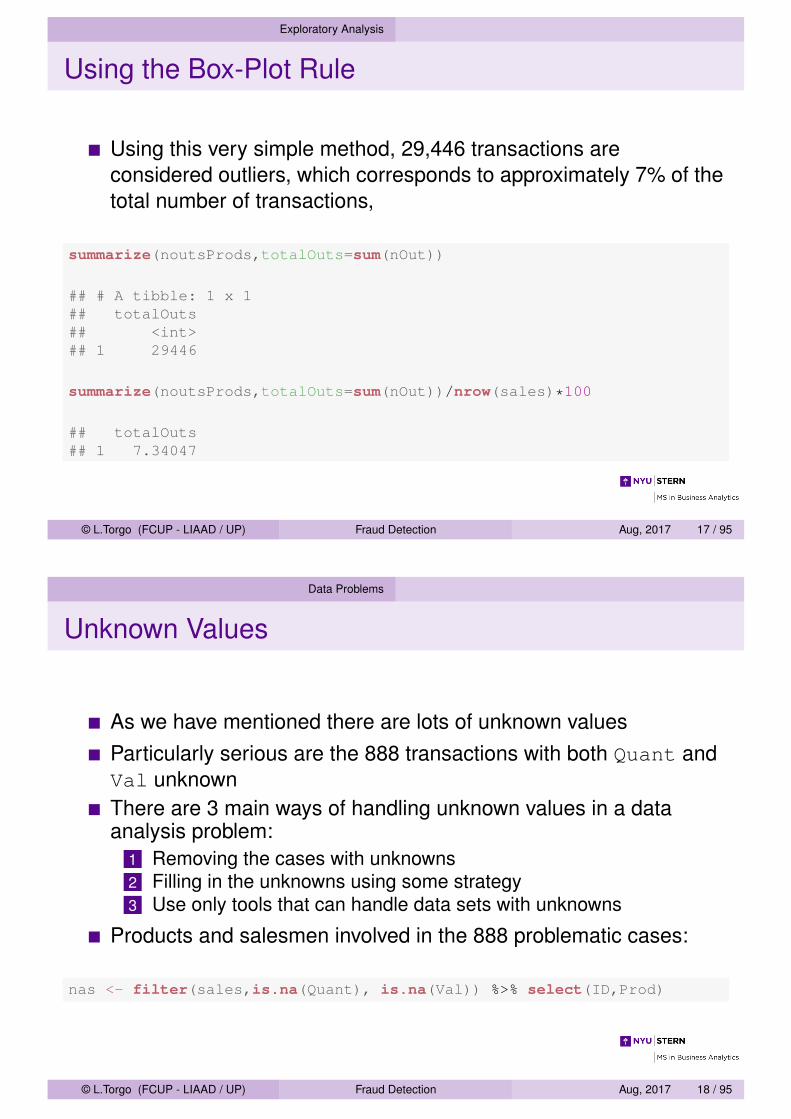
Using this very simple method, 29,446 transactions areconsidered outliers, which corresponds to approximately 7% of thetotal number of transactions,
summarize(noutsProds,totalOuts=sum(nOut))
## # A tibble: 1 x 1## totalOuts## <int>## 1 29446
summarize(noutsProds,totalOuts=sum(nOut))/nrow(sales)*100
## totalOuts## 1 7.34047
© L.Torgo (FCUP - LIAAD / UP) Fraud Detection Aug, 2017 17 / 95
Data Problems
Unknown Values
As we have mentioned there are lots of unknown valuesParticularly serious are the 888 transactions with both Quant andVal unknownThere are 3 main ways of handling unknown values in a dataanalysis problem:
1 Removing the cases with unknowns2 Filling in the unknowns using some strategy3 Use only tools that can handle data sets with unknowns
Products and salesmen involved in the 888 problematic cases:
nas <- filter(sales,is.na(Quant), is.na(Val)) %>% select(ID,Prod)
© L.Torgo (FCUP - LIAAD / UP) Fraud Detection Aug, 2017 18 / 95
Data Problems
The Problematic Products and Salesmen
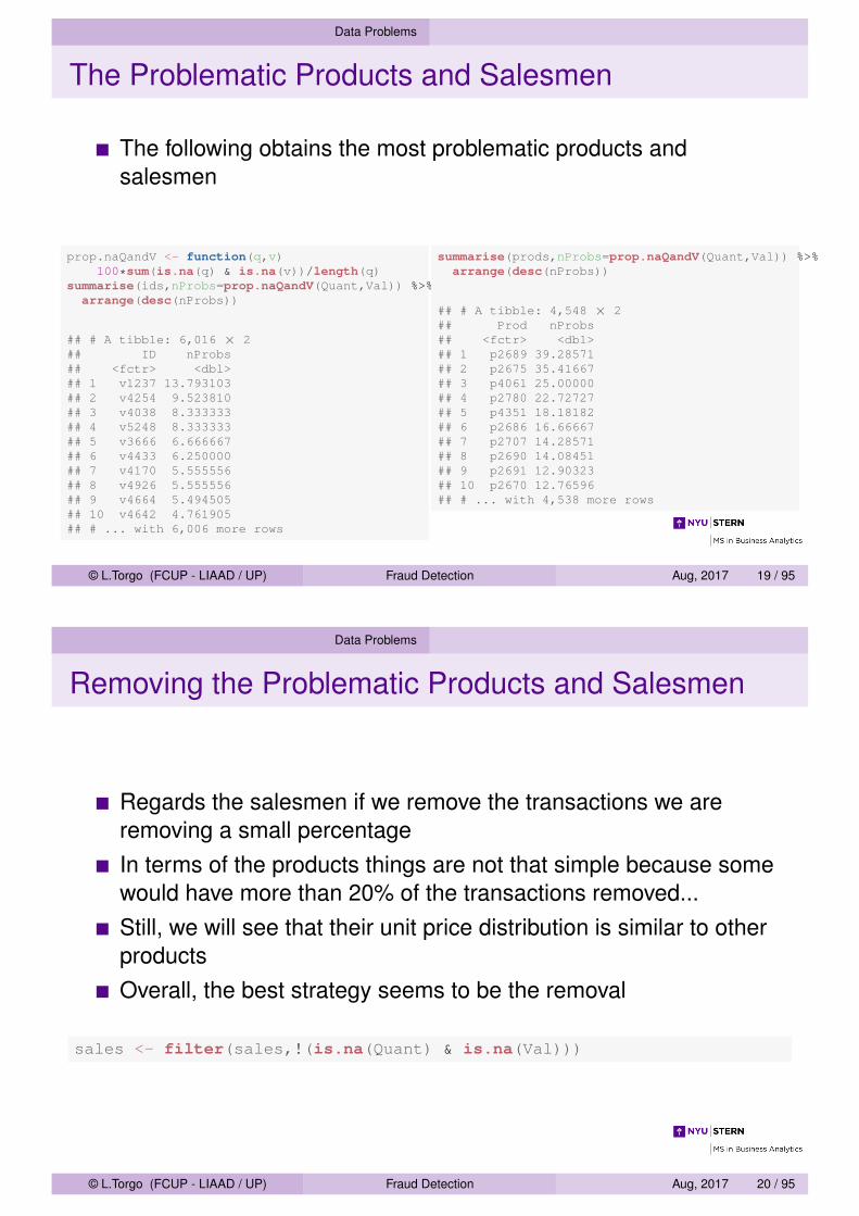
The following obtains the most problematic products andsalesmen
prop.naQandV <- function(q,v)100*sum(is.na(q) & is.na(v))/length(q)
summarise(ids,nProbs=prop.naQandV(Quant,Val)) %>%arrange(desc(nProbs))
## # A tibble: 6,016 × 2## ID nProbs## <fctr> <dbl>## 1 v1237 13.793103## 2 v4254 9.523810## 3 v4038 8.333333## 4 v5248 8.333333## 5 v3666 6.666667## 6 v4433 6.250000## 7 v4170 5.555556## 8 v4926 5.555556## 9 v4664 5.494505## 10 v4642 4.761905## # ... with 6,006 more rows
summarise(prods,nProbs=prop.naQandV(Quant,Val)) %>%arrange(desc(nProbs))
## # A tibble: 4,548 × 2## Prod nProbs## <fctr> <dbl>## 1 p2689 39.28571## 2 p2675 35.41667## 3 p4061 25.00000## 4 p2780 22.72727## 5 p4351 18.18182## 6 p2686 16.66667## 7 p2707 14.28571## 8 p2690 14.08451## 9 p2691 12.90323## 10 p2670 12.76596## # ... with 4,538 more rows
© L.Torgo (FCUP - LIAAD / UP) Fraud Detection Aug, 2017 19 / 95
Data Problems
Removing the Problematic Products and Salesmen
Regards the salesmen if we remove the transactions we areremoving a small percentageIn terms of the products things are not that simple because somewould have more than 20% of the transactions removed...Still, we will see that their unit price distribution is similar to otherproductsOverall, the best strategy seems to be the removal
sales <- filter(sales,!(is.na(Quant) & is.na(Val)))
© L.Torgo (FCUP - LIAAD / UP) Fraud Detection Aug, 2017 20 / 95
Data Problems
Handling the Remaining Unknowns
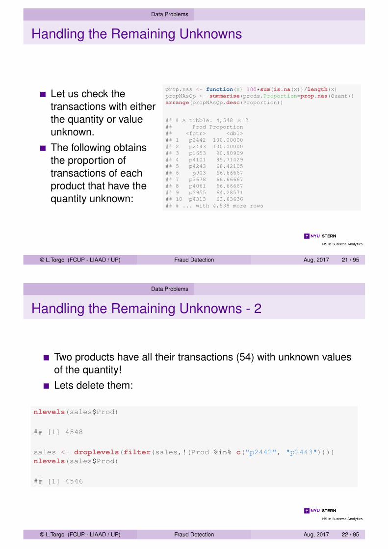
Let us check thetransactions with eitherthe quantity or valueunknown.The following obtainsthe proportion oftransactions of eachproduct that have thequantity unknown:
prop.nas <- function(x) 100*sum(is.na(x))/length(x)propNAsQp <- summarise(prods,Proportion=prop.nas(Quant))arrange(propNAsQp,desc(Proportion))
## # A tibble: 4,548 × 2## Prod Proportion## <fctr> <dbl>## 1 p2442 100.00000## 2 p2443 100.00000## 3 p1653 90.90909## 4 p4101 85.71429## 5 p4243 68.42105## 6 p903 66.66667## 7 p3678 66.66667## 8 p4061 66.66667## 9 p3955 64.28571## 10 p4313 63.63636## # ... with 4,538 more rows
© L.Torgo (FCUP - LIAAD / UP) Fraud Detection Aug, 2017 21 / 95
Data Problems
Handling the Remaining Unknowns - 2
Two products have all their transactions (54) with unknown valuesof the quantity!Lets delete them:
nlevels(sales$Prod)
## [1] 4548
sales <- droplevels(filter(sales,!(Prod %in% c("p2442", "p2443"))))nlevels(sales$Prod)
## [1] 4546
© L.Torgo (FCUP - LIAAD / UP) Fraud Detection Aug, 2017 22 / 95
Data Problems
Handling the Remaining Unknowns - 3
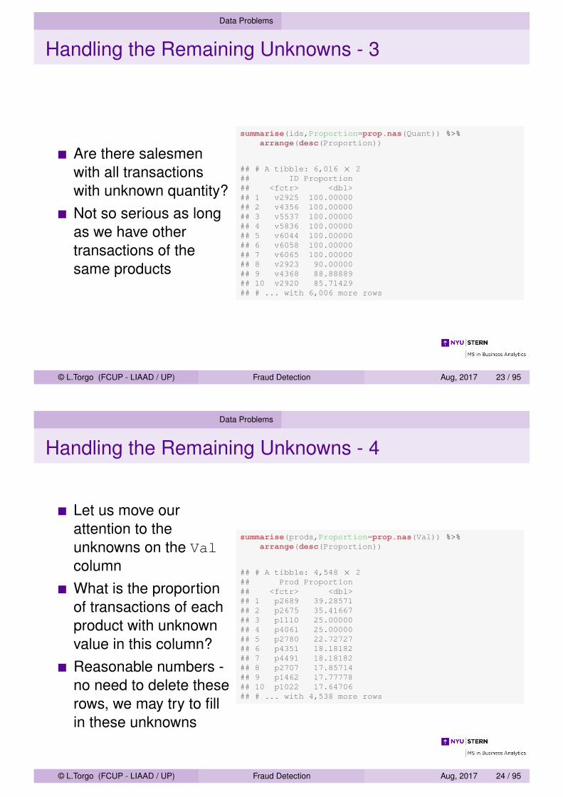
Are there salesmenwith all transactionswith unknown quantity?Not so serious as longas we have othertransactions of thesame products
summarise(ids,Proportion=prop.nas(Quant)) %>%arrange(desc(Proportion))
## # A tibble: 6,016 × 2## ID Proportion## <fctr> <dbl>## 1 v2925 100.00000## 2 v4356 100.00000## 3 v5537 100.00000## 4 v5836 100.00000## 5 v6044 100.00000## 6 v6058 100.00000## 7 v6065 100.00000## 8 v2923 90.00000## 9 v4368 88.88889## 10 v2920 85.71429## # ... with 6,006 more rows
© L.Torgo (FCUP - LIAAD / UP) Fraud Detection Aug, 2017 23 / 95
Data Problems
Handling the Remaining Unknowns - 4
Let us move ourattention to theunknowns on the ValcolumnWhat is the proportionof transactions of eachproduct with unknownvalue in this column?Reasonable numbers -no need to delete theserows, we may try to fillin these unknowns
summarise(prods,Proportion=prop.nas(Val)) %>%arrange(desc(Proportion))
## # A tibble: 4,548 × 2## Prod Proportion## <fctr> <dbl>## 1 p2689 39.28571## 2 p2675 35.41667## 3 p1110 25.00000## 4 p4061 25.00000## 5 p2780 22.72727## 6 p4351 18.18182## 7 p4491 18.18182## 8 p2707 17.85714## 9 p1462 17.77778## 10 p1022 17.64706## # ... with 4,538 more rows
© L.Torgo (FCUP - LIAAD / UP) Fraud Detection Aug, 2017 24 / 95
Data Problems
Handling the Remaining Unknowns - 5
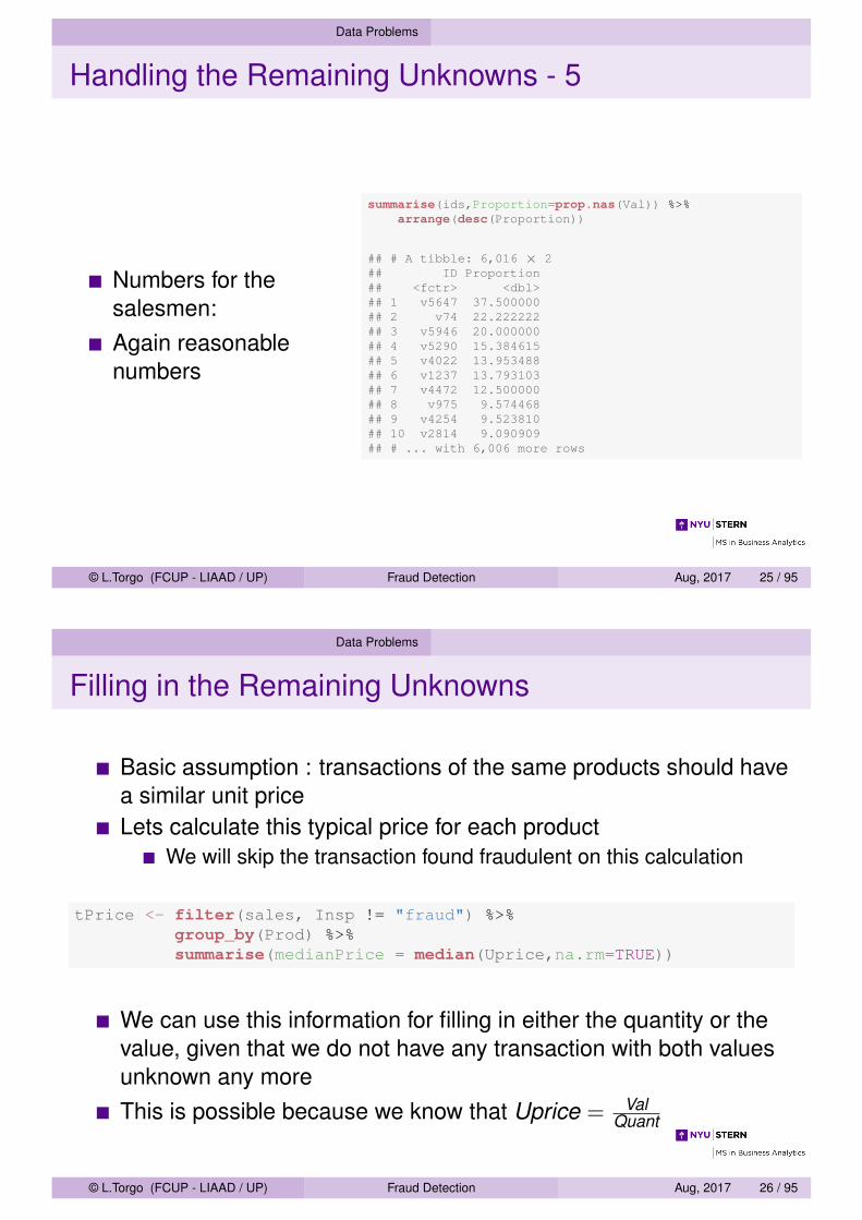
Numbers for thesalesmen:Again reasonablenumbers
summarise(ids,Proportion=prop.nas(Val)) %>%arrange(desc(Proportion))
## # A tibble: 6,016 × 2## ID Proportion## <fctr> <dbl>## 1 v5647 37.500000## 2 v74 22.222222## 3 v5946 20.000000## 4 v5290 15.384615## 5 v4022 13.953488## 6 v1237 13.793103## 7 v4472 12.500000## 8 v975 9.574468## 9 v4254 9.523810## 10 v2814 9.090909## # ... with 6,006 more rows
© L.Torgo (FCUP - LIAAD / UP) Fraud Detection Aug, 2017 25 / 95
Data Problems
Filling in the Remaining Unknowns
Basic assumption : transactions of the same products should havea similar unit priceLets calculate this typical price for each product
We will skip the transaction found fraudulent on this calculation
tPrice <- filter(sales, Insp != "fraud") %>%group_by(Prod) %>%summarise(medianPrice = median(Uprice,na.rm=TRUE))
We can use this information for filling in either the quantity or thevalue, given that we do not have any transaction with both valuesunknown any moreThis is possible because we know that Uprice = Val
Quant
© L.Torgo (FCUP - LIAAD / UP) Fraud Detection Aug, 2017 26 / 95

Data Problems
Filling in the Remaining Unknowns - 2
The following code fills in the remaining unknowns
noQuantMedPrices <- filter(sales, is.na(Quant)) %>%inner_join(tPrice) %>% select(medianPrice)
noValMedPrices <- filter(sales, is.na(Val)) %>%inner_join(tPrice) %>% select(medianPrice)
noQuant <- which(is.na(sales$Quant))noVal <- which(is.na(sales$Val))sales[noQuant,'Quant'] <- ceiling(sales[noQuant,'Val']/noQuantMedPrices)sales[noVal,'Val'] <- sales[noVal,'Quant'] * noValMedPrices
sales$Uprice <- sales$Val/sales$Quant
© L.Torgo (FCUP - LIAAD / UP) Fraud Detection Aug, 2017 27 / 95
Hands On Exploratory Analysis
Hands On Exploratory Analysis
Get your hands on this case study by carrying out most of thesteps that were illustrated and by trying alternative pathsTry to tick these objectives:
1 Explore the data and understand it2 Understand how dplyr works3 Take care of the unknown values4 In the end of your steps save the resulting object in a file for later
usagesave(sales,file="mySalesObj.Rdata")
Note: you should produce a report from your analysis using Rmarkdown Notebooks in RStudio
© L.Torgo (FCUP - LIAAD / UP) Fraud Detection Aug, 2017 28 / 95
Possible Approaches
Different Approaches to the Data Mining Task
The target variable (the Insp column) has three values: ok,fraud and unkn
The value unkn means that those transactions were not inspectedand thus may be either frauds or normal transactions (OK)In a way this represents an unknown value of the target variableIn these contexts there are essentially 3 ways of addressing thesetasks:
Using unsupervised techniquesUsing supervised techniquesUsing semi-supervised techniques
© L.Torgo (FCUP - LIAAD / UP) Fraud Detection Aug, 2017 29 / 95
Possible Approaches
Unsupervised Techniques
Assume complete ignorance of the target variable valuesTry to find the natural groupings of the dataThe reasoning is that fraudulent transactions should be differentfrom normal transactions, i.e. should belong to different groups ofdataUsing them would mean to throw away all information contained incolumn Insp
© L.Torgo (FCUP - LIAAD / UP) Fraud Detection Aug, 2017 30 / 95
Possible Approaches
Supervised Techniques
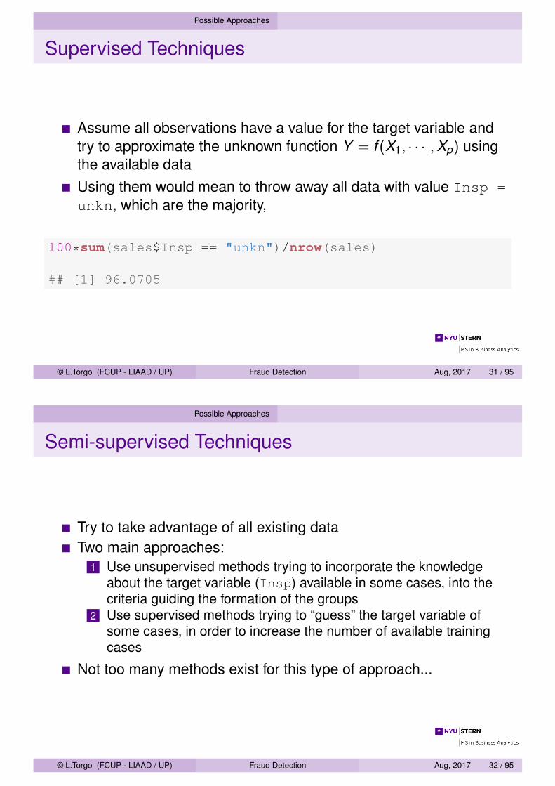
Assume all observations have a value for the target variable andtry to approximate the unknown function Y = f (X1, · · · ,Xp) usingthe available dataUsing them would mean to throw away all data with value Insp =unkn, which are the majority,
100*sum(sales$Insp == "unkn")/nrow(sales)
## [1] 96.0705
© L.Torgo (FCUP - LIAAD / UP) Fraud Detection Aug, 2017 31 / 95
Possible Approaches
Semi-supervised Techniques
Try to take advantage of all existing dataTwo main approaches:
1 Use unsupervised methods trying to incorporate the knowledgeabout the target variable (Insp) available in some cases, into thecriteria guiding the formation of the groups
2 Use supervised methods trying to “guess” the target variable ofsome cases, in order to increase the number of available trainingcases
Not too many methods exist for this type of approach...
© L.Torgo (FCUP - LIAAD / UP) Fraud Detection Aug, 2017 32 / 95
Evaluation Criteria
Goals of the Data Mining Task
Inspection/auditing activities are typically constrained by limitedresourcesInspecting all cases is usually not possibleIn this context, the best outcome from a data mining tool is aninspection rankingThis type of result allows users to allocate their (limited) resourcesto the most promising cases and stop when necessary
© L.Torgo (FCUP - LIAAD / UP) Fraud Detection Aug, 2017 33 / 95
Evaluation Criteria
How to Evaluate the Results?
Before checking how to obtain inspection rankings let us see howto evaluate this type of outputOur application has an additional difficulty - labeled and unlabeledcasesIf an unlabeled case appears in the top positions of the inspectionranking how to know if this is correct?
© L.Torgo (FCUP - LIAAD / UP) Fraud Detection Aug, 2017 34 / 95
Evaluation Criteria Precision/Recall
Precision/Recall
Frauds are rare eventsThe Precision/Recall evaluation setting allows us to focus on theperformance of a model on a specific class (in this case thefrauds)Precision will be measured as the proportion of cases the modelssay are fraudulent that are effectively fraudsRecall will be measured as the proportion of frauds that aresignaled by the models as such
© L.Torgo (FCUP - LIAAD / UP) Fraud Detection Aug, 2017 35 / 95
Evaluation Criteria Precision/Recall
Precision/Recall
Usually there is a trade-off between precision and recall - it is easyto get 100% recall by forecasting all cases as fraudsIn a setting with limited inspection resources what we really aim atis to maximize the use of these resourcesRecall is the key issue on this application - we want to capture asmany frauds as possible with our limited inspection resources
© L.Torgo (FCUP - LIAAD / UP) Fraud Detection Aug, 2017 36 / 95
Evaluation Criteria Precision/Recall
Precision/Recall Curves
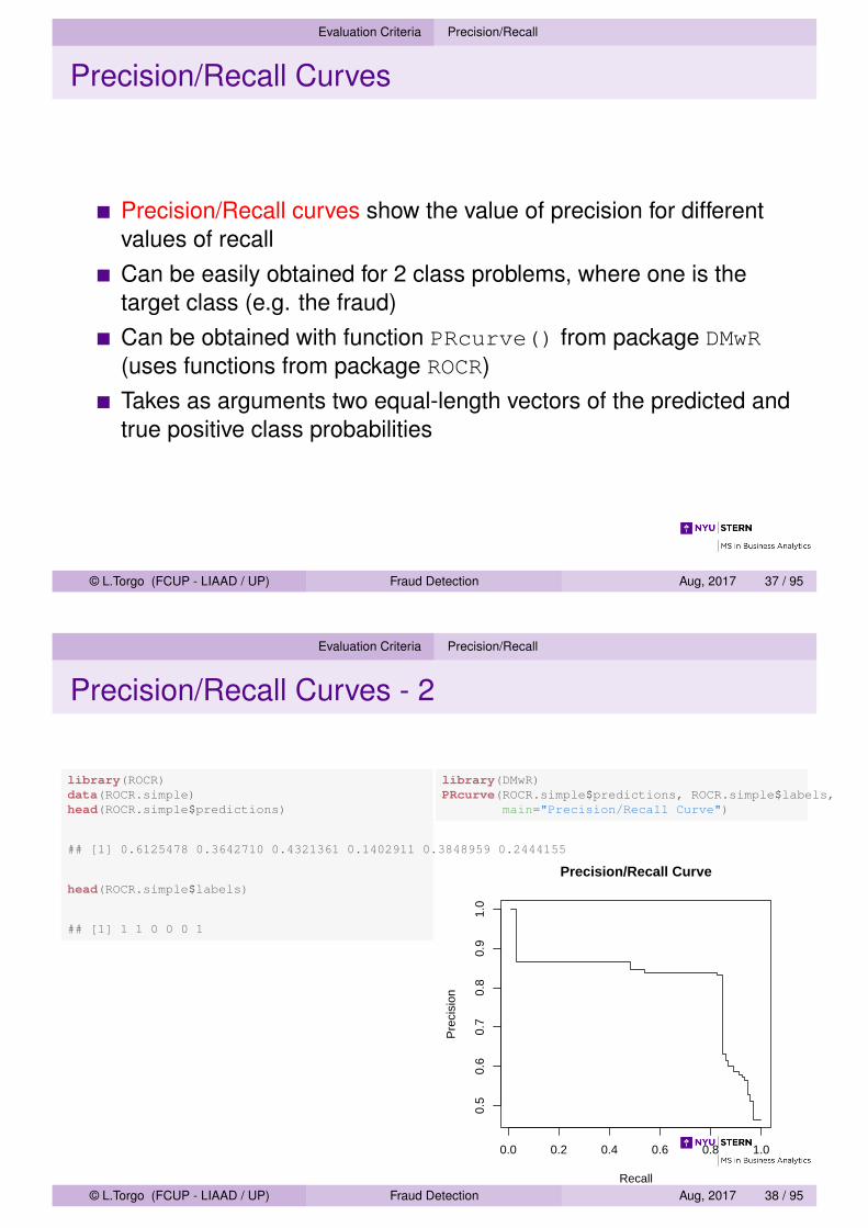
Precision/Recall curves show the value of precision for differentvalues of recallCan be easily obtained for 2 class problems, where one is thetarget class (e.g. the fraud)Can be obtained with function PRcurve() from package DMwR(uses functions from package ROCR)Takes as arguments two equal-length vectors of the predicted andtrue positive class probabilities
© L.Torgo (FCUP - LIAAD / UP) Fraud Detection Aug, 2017 37 / 95
Evaluation Criteria Precision/Recall
Precision/Recall Curves - 2
library(ROCR)data(ROCR.simple)head(ROCR.simple$predictions)
## [1] 0.6125478 0.3642710 0.4321361 0.1402911 0.3848959 0.2444155
head(ROCR.simple$labels)
## [1] 1 1 0 0 0 1
library(DMwR)PRcurve(ROCR.simple$predictions, ROCR.simple$labels,
main="Precision/Recall Curve")
Precision/Recall Curve
Recall
Pre
cisi
on
0.0 0.2 0.4 0.6 0.8 1.0
0.5
0.6
0.7
0.8
0.9
1.0
© L.Torgo (FCUP - LIAAD / UP) Fraud Detection Aug, 2017 38 / 95
Evaluation Criteria Precision/Recall
Lift Charts
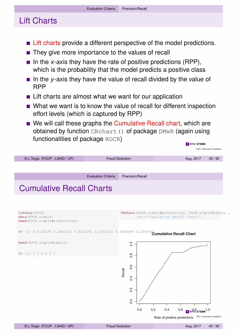
Lift charts provide a different perspective of the model predictions.They give more importance to the values of recallIn the x-axis they have the rate of positive predictions (RPP),which is the probability that the model predicts a positive classIn the y -axis they have the value of recall divided by the value ofRPPLift charts are almost what we want for our applicationWhat we want is to know the value of recall for different inspectioneffort levels (which is captured by RPP)We will call these graphs the Cumulative Recall chart, which areobtained by function CRchart() of package DMwR (again usingfunctionalities of package ROCR)
© L.Torgo (FCUP - LIAAD / UP) Fraud Detection Aug, 2017 39 / 95
Evaluation Criteria Precision/Recall
Cumulative Recall Charts
library(ROCR)data(ROCR.simple)head(ROCR.simple$predictions)
## [1] 0.6125478 0.3642710 0.4321361 0.1402911 0.3848959 0.2444155
head(ROCR.simple$labels)
## [1] 1 1 0 0 0 1
CRchart(ROCR.simple$predictions, ROCR.simple$labels ,main='Cumulative Recall Chart')
Cumulative Recall Chart
Rate of positive predictions
Rec
all
0.0 0.2 0.4 0.6 0.8 1.0
0.0
0.2
0.4
0.6
0.8
1.0
© L.Torgo (FCUP - LIAAD / UP) Fraud Detection Aug, 2017 40 / 95
Evaluation Criteria Normalized Distance to Typical Price
Normalized Distance to Typical Price
Previous measures only evaluate the quality of rankings in termsof the labeled transactions - supervised metricsThe obtained rankings will surely contain unlabeled transactionreports - are these good inspection recommendations?We can compare their unit price with the typical price of thereports of the same productWe would expect that the difference between these prices is high,as this is an indication that something is wrong with the report
© L.Torgo (FCUP - LIAAD / UP) Fraud Detection Aug, 2017 41 / 95
Evaluation Criteria Normalized Distance to Typical Price
Normalized Distance to Typical Price
We propose to use the Normalized Distance to Typical Price (NDTPp)to measure this difference
NDTPp(u) =|u − Up|
IQRp
where Up is the typical price of product p (measured by the median),and IQRp is the respective inter-quartile rangeThe higher the value of NDTP the stranger is the unit price of atransaction, and thus the better the recommendation for inspection.
© L.Torgo (FCUP - LIAAD / UP) Fraud Detection Aug, 2017 42 / 95
Evaluation Criteria Normalized Distance to Typical Price
Normalized Distance to Typical Price - 2
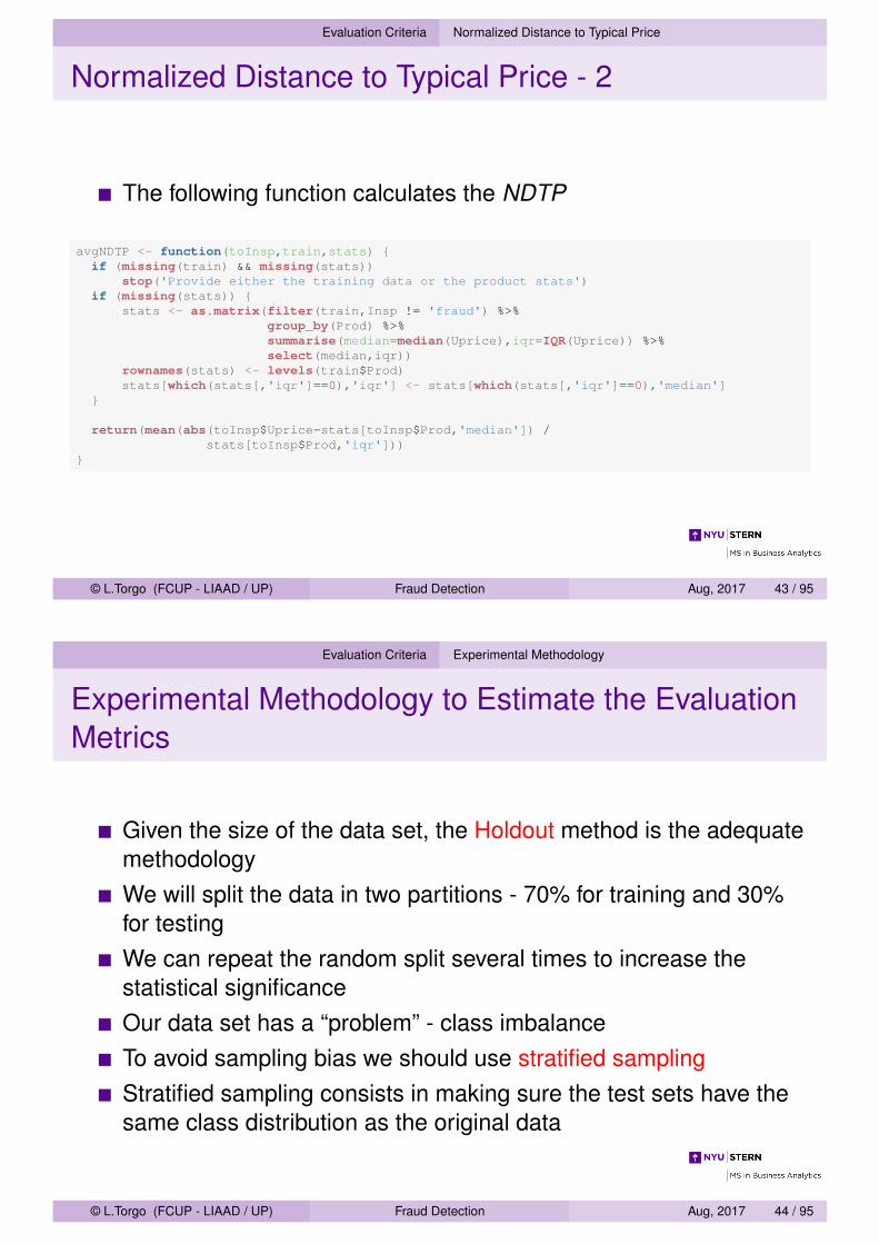
The following function calculates the NDTP
avgNDTP <- function(toInsp,train,stats) {if (missing(train) && missing(stats))
stop('Provide either the training data or the product stats')if (missing(stats)) {
stats <- as.matrix(filter(train,Insp != 'fraud') %>%group_by(Prod) %>%summarise(median=median(Uprice),iqr=IQR(Uprice)) %>%select(median,iqr))
rownames(stats) <- levels(train$Prod)stats[which(stats[,'iqr']==0),'iqr'] <- stats[which(stats[,'iqr']==0),'median']
}
return(mean(abs(toInsp$Uprice-stats[toInsp$Prod,'median']) /stats[toInsp$Prod,'iqr']))
}
© L.Torgo (FCUP - LIAAD / UP) Fraud Detection Aug, 2017 43 / 95
Evaluation Criteria Experimental Methodology
Experimental Methodology to Estimate the EvaluationMetrics
Given the size of the data set, the Holdout method is the adequatemethodologyWe will split the data in two partitions - 70% for training and 30%for testingWe can repeat the random split several times to increase thestatistical significanceOur data set has a “problem” - class imbalanceTo avoid sampling bias we should use stratified samplingStratified sampling consists in making sure the test sets have thesame class distribution as the original data
© L.Torgo (FCUP - LIAAD / UP) Fraud Detection Aug, 2017 44 / 95
Evaluation Criteria Experimental Methodology
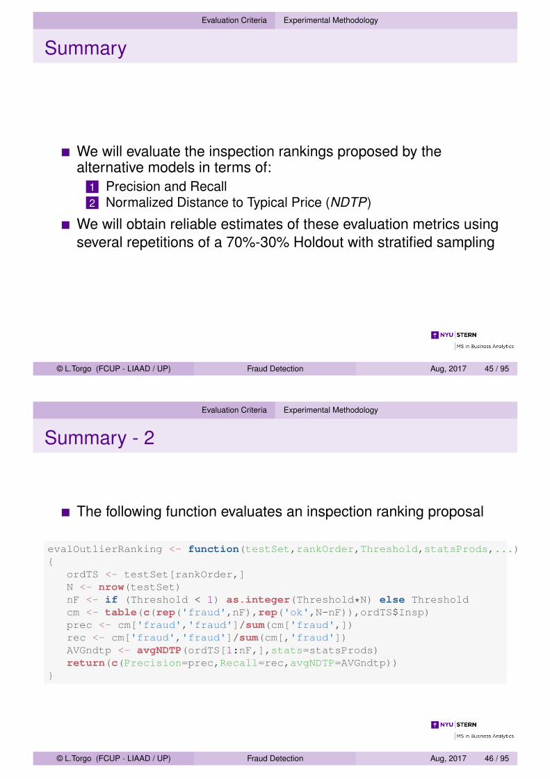
Summary
We will evaluate the inspection rankings proposed by thealternative models in terms of:
1 Precision and Recall2 Normalized Distance to Typical Price (NDTP)
We will obtain reliable estimates of these evaluation metrics usingseveral repetitions of a 70%-30% Holdout with stratified sampling
© L.Torgo (FCUP - LIAAD / UP) Fraud Detection Aug, 2017 45 / 95
Evaluation Criteria Experimental Methodology
Summary - 2
The following function evaluates an inspection ranking proposal
evalOutlierRanking <- function(testSet,rankOrder,Threshold,statsProds,...){
ordTS <- testSet[rankOrder,]N <- nrow(testSet)nF <- if (Threshold < 1) as.integer(Threshold*N) else Thresholdcm <- table(c(rep('fraud',nF),rep('ok',N-nF)),ordTS$Insp)prec <- cm['fraud','fraud']/sum(cm['fraud',])rec <- cm['fraud','fraud']/sum(cm[,'fraud'])AVGndtp <- avgNDTP(ordTS[1:nF,],stats=statsProds)return(c(Precision=prec,Recall=rec,avgNDTP=AVGndtp))
}
© L.Torgo (FCUP - LIAAD / UP) Fraud Detection Aug, 2017 46 / 95
Evaluation Criteria Experimental Methodology
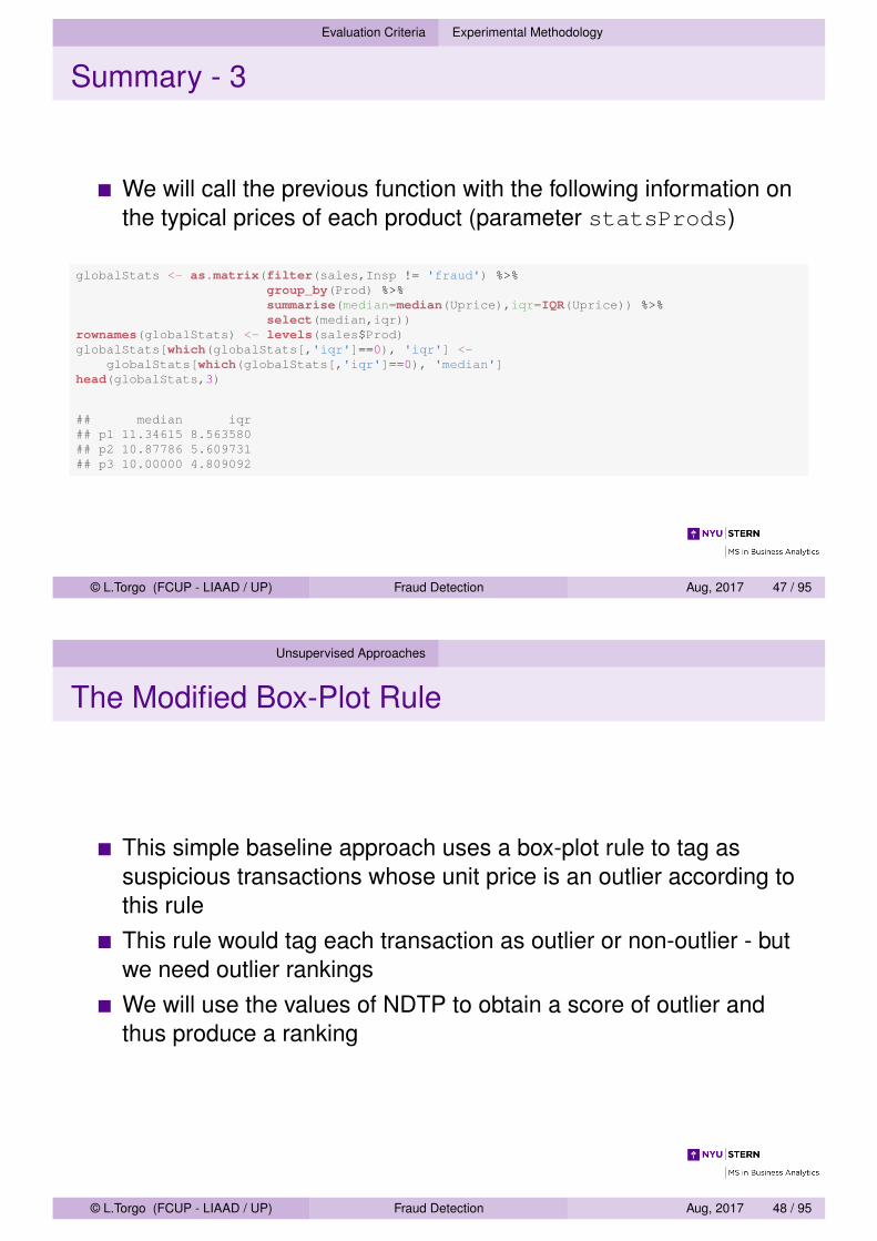
Summary - 3
We will call the previous function with the following information onthe typical prices of each product (parameter statsProds)
globalStats <- as.matrix(filter(sales,Insp != 'fraud') %>%group_by(Prod) %>%summarise(median=median(Uprice),iqr=IQR(Uprice)) %>%select(median,iqr))
rownames(globalStats) <- levels(sales$Prod)globalStats[which(globalStats[,'iqr']==0), 'iqr'] <-
globalStats[which(globalStats[,'iqr']==0), 'median']head(globalStats,3)
## median iqr## p1 11.34615 8.563580## p2 10.87786 5.609731## p3 10.00000 4.809092
© L.Torgo (FCUP - LIAAD / UP) Fraud Detection Aug, 2017 47 / 95
Unsupervised Approaches
The Modified Box-Plot Rule
This simple baseline approach uses a box-plot rule to tag assuspicious transactions whose unit price is an outlier according tothis ruleThis rule would tag each transaction as outlier or non-outlier - butwe need outlier rankingsWe will use the values of NDTP to obtain a score of outlier andthus produce a ranking
© L.Torgo (FCUP - LIAAD / UP) Fraud Detection Aug, 2017 48 / 95

Unsupervised Approaches
Evaluation of the Modified Box-Plot Rule
We will use the performanceEstimation package to estimatethe scores of the selected metrics (precision, recall and NDTP)Estimates will be obtained using an Holdout experiment leaving30% of the cases as test setWe will repeat the (random) train+test split 3 times to increase thesignificance of our estimatesWe will calculate our metrics assuming that we can only audit 10%of the test set
© L.Torgo (FCUP - LIAAD / UP) Fraud Detection Aug, 2017 49 / 95
Unsupervised Approaches
The Workflow implementing the modified Box-PlotRule
BPrule.wf <- function(form,train,test,...) {require(dplyr, quietly=TRUE)ms <- as.matrix(filter(train,Insp != 'fraud') %>%
group_by(Prod) %>%summarise(median=median(Uprice),iqr=IQR(Uprice)) %>%select(median,iqr))
rownames(ms) <- levels(train$Prod)ms[which(ms[,'iqr']==0),'iqr'] <- ms[which(ms[,'iqr']==0),'median']ORscore <- abs(test$Uprice-ms[test$Prod,'median']) /
ms[test$Prod,'iqr']rankOrder <- order(ORscore,decreasing=T)res <- list(testSet=test,rankOrder=rankOrder,
probs=matrix(c(ORscore,ifelse(test$Insp=='fraud',1,0)),ncol=2))
res}
© L.Torgo (FCUP - LIAAD / UP) Fraud Detection Aug, 2017 50 / 95
Unsupervised Approaches
Evaluating the Modified Box-Plot Rule
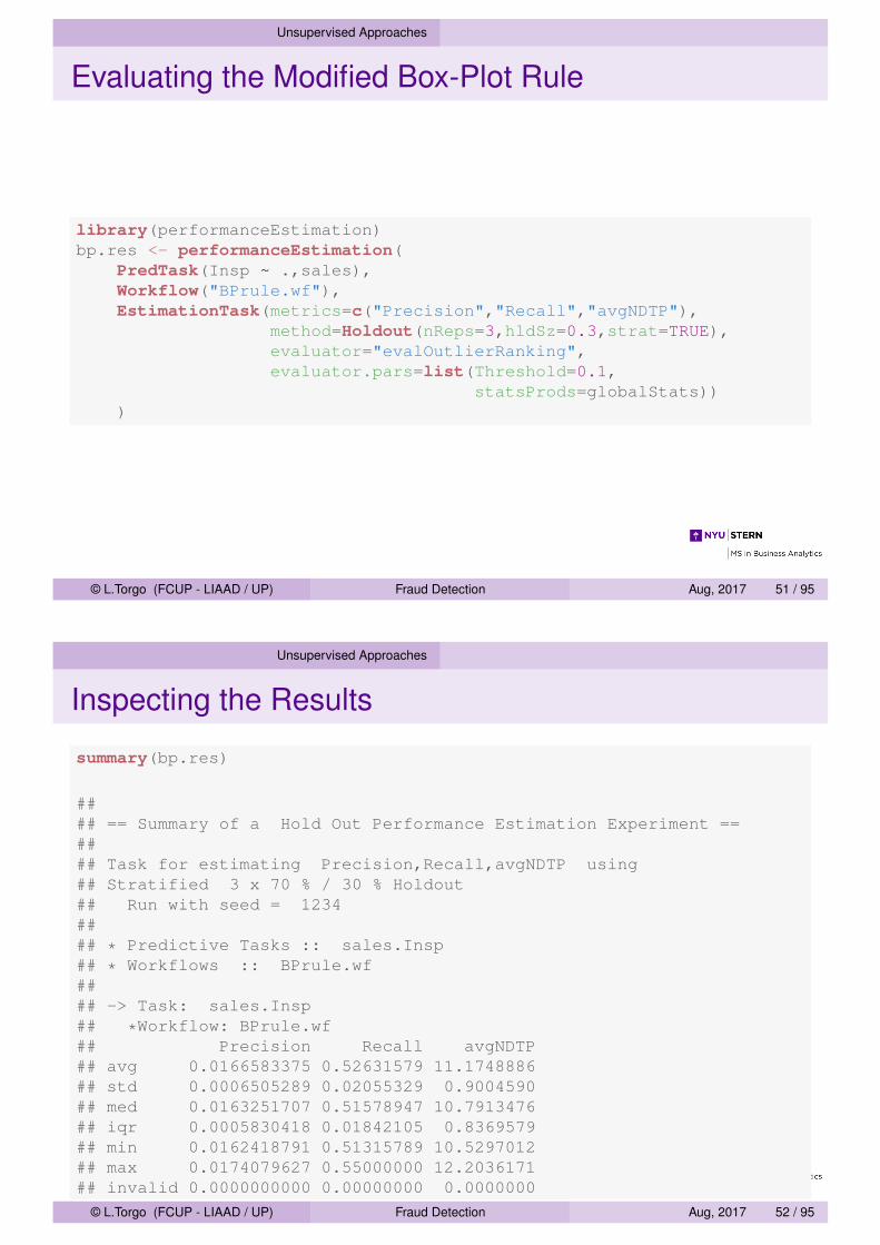
library(performanceEstimation)bp.res <- performanceEstimation(
PredTask(Insp ~ .,sales),Workflow("BPrule.wf"),EstimationTask(metrics=c("Precision","Recall","avgNDTP"),
method=Holdout(nReps=3,hldSz=0.3,strat=TRUE),evaluator="evalOutlierRanking",evaluator.pars=list(Threshold=0.1,
statsProds=globalStats)))
© L.Torgo (FCUP - LIAAD / UP) Fraud Detection Aug, 2017 51 / 95
Unsupervised Approaches
Inspecting the Results
summary(bp.res)
#### == Summary of a Hold Out Performance Estimation Experiment ==#### Task for estimating Precision,Recall,avgNDTP using## Stratified 3 x 70 % / 30 % Holdout## Run with seed = 1234#### * Predictive Tasks :: sales.Insp## * Workflows :: BPrule.wf#### -> Task: sales.Insp## *Workflow: BPrule.wf## Precision Recall avgNDTP## avg 0.0166583375 0.52631579 11.1748886## std 0.0006505289 0.02055329 0.9004590## med 0.0163251707 0.51578947 10.7913476## iqr 0.0005830418 0.01842105 0.8369579## min 0.0162418791 0.51315789 10.5297012## max 0.0174079627 0.55000000 12.2036171## invalid 0.0000000000 0.00000000 0.0000000
© L.Torgo (FCUP - LIAAD / UP) Fraud Detection Aug, 2017 52 / 95
Unsupervised Approaches
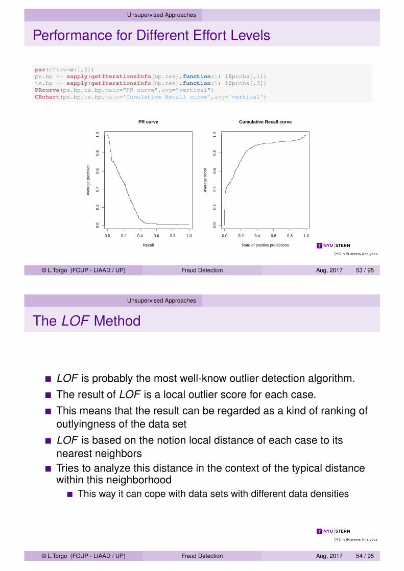
Performance for Different Effort Levels
par(mfrow=c(1,2))ps.bp <- sapply(getIterationsInfo(bp.res),function(i) i$probs[,1])ts.bp <- sapply(getIterationsInfo(bp.res),function(i) i$probs[,2])PRcurve(ps.bp,ts.bp,main="PR curve",avg="vertical")CRchart(ps.bp,ts.bp,main='Cumulative Recall curve',avg='vertical')
PR curve
Recall
Ave
rage
pre
cisi
on
0.0 0.2 0.4 0.6 0.8 1.0
0.0
0.2
0.4
0.6
0.8
1.0
Cumulative Recall curve
Rate of positive predictions
Ave
rage
rec
all
0.0 0.2 0.4 0.6 0.8 1.0
0.0
0.2
0.4
0.6
0.8
1.0
© L.Torgo (FCUP - LIAAD / UP) Fraud Detection Aug, 2017 53 / 95
Unsupervised Approaches
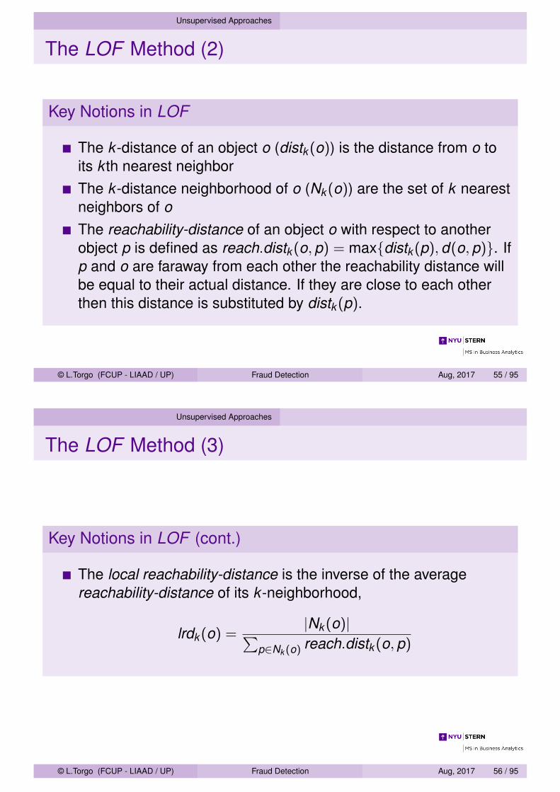
The LOF Method
LOF is probably the most well-know outlier detection algorithm.The result of LOF is a local outlier score for each case.This means that the result can be regarded as a kind of ranking ofoutlyingness of the data setLOF is based on the notion local distance of each case to itsnearest neighborsTries to analyze this distance in the context of the typical distancewithin this neighborhood
This way it can cope with data sets with different data densities
© L.Torgo (FCUP - LIAAD / UP) Fraud Detection Aug, 2017 54 / 95
Unsupervised Approaches
The LOF Method (2)
Key Notions in LOF
The k -distance of an object o (distk (o)) is the distance from o toits k th nearest neighborThe k -distance neighborhood of o (Nk (o)) are the set of k nearestneighbors of oThe reachability-distance of an object o with respect to anotherobject p is defined as reach.distk (o,p) = max{distk (p),d(o,p)}. Ifp and o are faraway from each other the reachability distance willbe equal to their actual distance. If they are close to each otherthen this distance is substituted by distk (p).
© L.Torgo (FCUP - LIAAD / UP) Fraud Detection Aug, 2017 55 / 95
Unsupervised Approaches
The LOF Method (3)
Key Notions in LOF (cont.)
The local reachability-distance is the inverse of the averagereachability-distance of its k -neighborhood,
lrdk (o) =|Nk (o)|∑
p∈Nk (o) reach.distk (o,p)
© L.Torgo (FCUP - LIAAD / UP) Fraud Detection Aug, 2017 56 / 95
Unsupervised Approaches
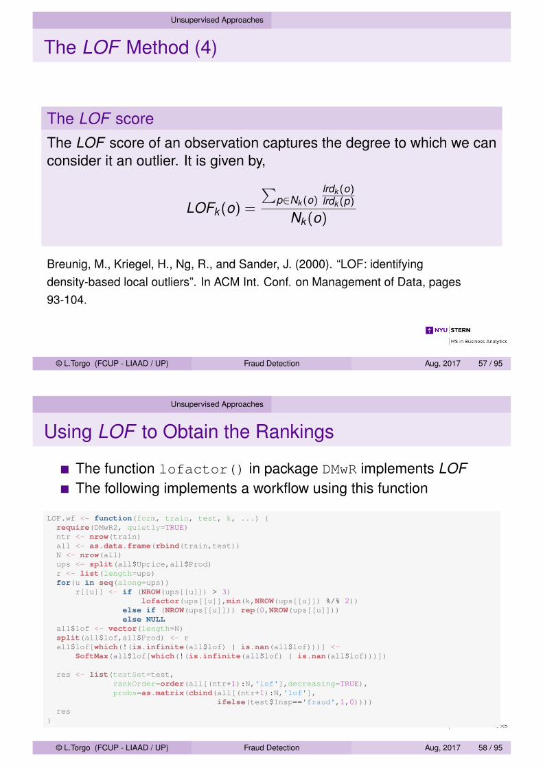
The LOF Method (4)
The LOF scoreThe LOF score of an observation captures the degree to which we canconsider it an outlier. It is given by,
LOFk (o) =
∑p∈Nk (o)
lrdk (o)lrdk (p)
Nk (o)
Breunig, M., Kriegel, H., Ng, R., and Sander, J. (2000). “LOF: identifyingdensity-based local outliers”. In ACM Int. Conf. on Management of Data, pages93-104.
© L.Torgo (FCUP - LIAAD / UP) Fraud Detection Aug, 2017 57 / 95
Unsupervised Approaches
Using LOF to Obtain the Rankings
The function lofactor() in package DMwR implements LOFThe following implements a workflow using this function
LOF.wf <- function(form, train, test, k, ...) {require(DMwR2, quietly=TRUE)ntr <- nrow(train)all <- as.data.frame(rbind(train,test))N <- nrow(all)ups <- split(all$Uprice,all$Prod)r <- list(length=ups)for(u in seq(along=ups))
r[[u]] <- if (NROW(ups[[u]]) > 3)lofactor(ups[[u]],min(k,NROW(ups[[u]]) %/% 2))
else if (NROW(ups[[u]])) rep(0,NROW(ups[[u]]))else NULL
all$lof <- vector(length=N)split(all$lof,all$Prod) <- rall$lof[which(!(is.infinite(all$lof) | is.nan(all$lof)))] <-
SoftMax(all$lof[which(!(is.infinite(all$lof) | is.nan(all$lof)))])
res <- list(testSet=test,rankOrder=order(all[(ntr+1):N,'lof'],decreasing=TRUE),probs=as.matrix(cbind(all[(ntr+1):N,'lof'],
ifelse(test$Insp=='fraud',1,0))))res
}
© L.Torgo (FCUP - LIAAD / UP) Fraud Detection Aug, 2017 58 / 95
Unsupervised Approaches
Evaluating the LOF Method
lof.res <- performanceEstimation(PredTask(Insp ~ .,sales),Workflow("LOF.wf",k=7),EstimationTask(metrics=c("Precision","Recall","avgNDTP"),
method=Holdout(nReps=3,hldSz=0.3,strat=TRUE),evaluator="evalOutlierRanking",evaluator.pars=list(Threshold=0.1,
statsProds=globalStats)))
© L.Torgo (FCUP - LIAAD / UP) Fraud Detection Aug, 2017 59 / 95
Unsupervised Approaches
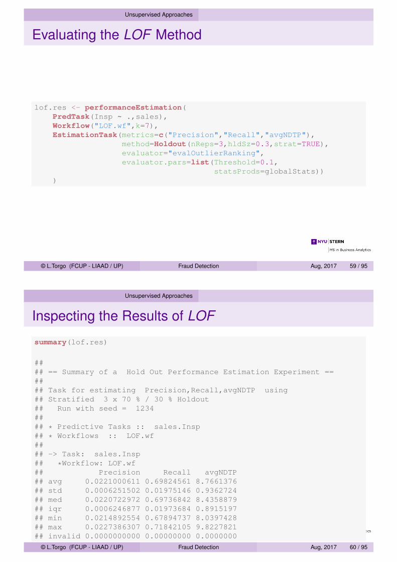
Inspecting the Results of LOF
summary(lof.res)
#### == Summary of a Hold Out Performance Estimation Experiment ==#### Task for estimating Precision,Recall,avgNDTP using## Stratified 3 x 70 % / 30 % Holdout## Run with seed = 1234#### * Predictive Tasks :: sales.Insp## * Workflows :: LOF.wf#### -> Task: sales.Insp## *Workflow: LOF.wf## Precision Recall avgNDTP## avg 0.0221000611 0.69824561 8.7661376## std 0.0006251502 0.01975146 0.9362724## med 0.0220722972 0.69736842 8.4358879## iqr 0.0006246877 0.01973684 0.8915197## min 0.0214892554 0.67894737 8.0397428## max 0.0227386307 0.71842105 9.8227821## invalid 0.0000000000 0.00000000 0.0000000
© L.Torgo (FCUP - LIAAD / UP) Fraud Detection Aug, 2017 60 / 95
Unsupervised Approaches
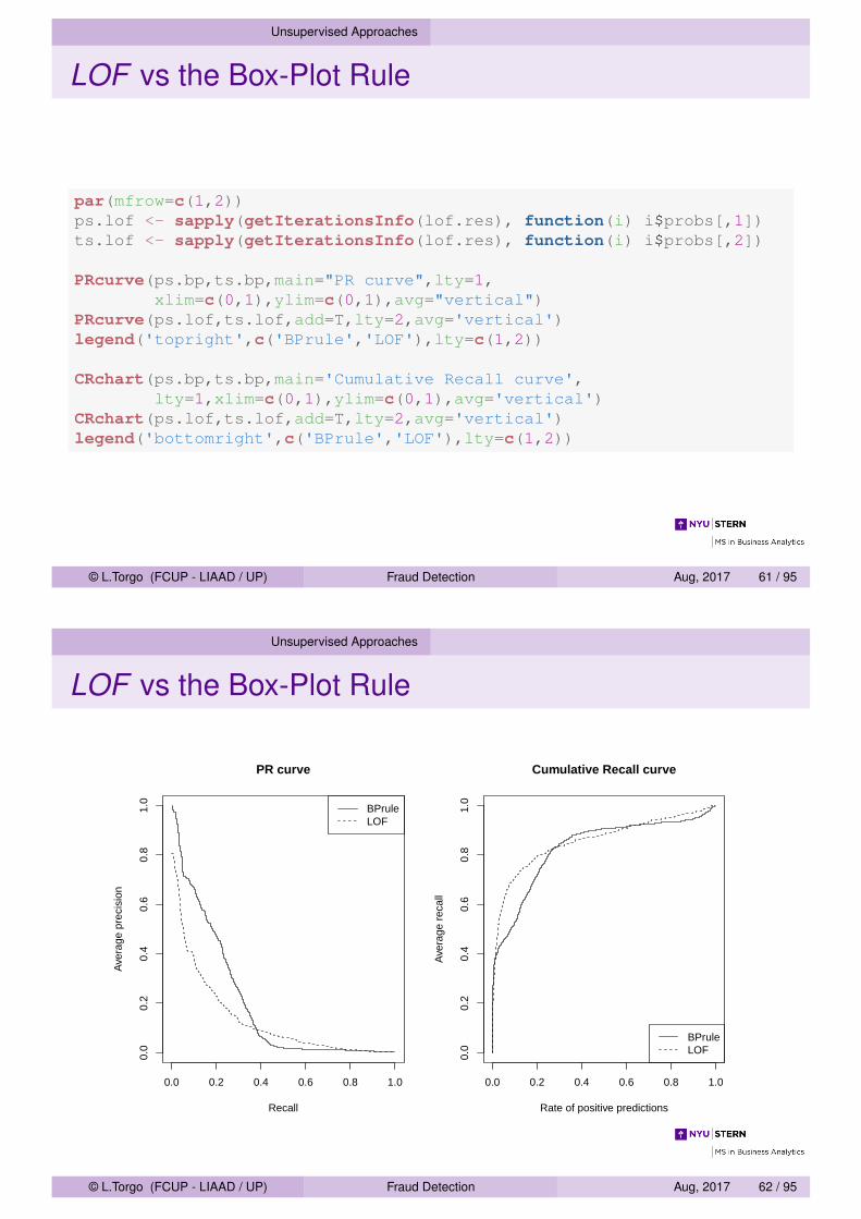
LOF vs the Box-Plot Rule
par(mfrow=c(1,2))ps.lof <- sapply(getIterationsInfo(lof.res), function(i) i$probs[,1])ts.lof <- sapply(getIterationsInfo(lof.res), function(i) i$probs[,2])
PRcurve(ps.bp,ts.bp,main="PR curve",lty=1,xlim=c(0,1),ylim=c(0,1),avg="vertical")
PRcurve(ps.lof,ts.lof,add=T,lty=2,avg='vertical')legend('topright',c('BPrule','LOF'),lty=c(1,2))
CRchart(ps.bp,ts.bp,main='Cumulative Recall curve',lty=1,xlim=c(0,1),ylim=c(0,1),avg='vertical')
CRchart(ps.lof,ts.lof,add=T,lty=2,avg='vertical')legend('bottomright',c('BPrule','LOF'),lty=c(1,2))
© L.Torgo (FCUP - LIAAD / UP) Fraud Detection Aug, 2017 61 / 95
Unsupervised Approaches
LOF vs the Box-Plot Rule
PR curve
Recall
Ave
rage
pre
cisi
on
0.0 0.2 0.4 0.6 0.8 1.0
0.0
0.2
0.4
0.6
0.8
1.0
BPruleLOF
Cumulative Recall curve
Rate of positive predictions
Ave
rage
rec
all
0.0 0.2 0.4 0.6 0.8 1.0
0.0
0.2
0.4
0.6
0.8
1.0
BPruleLOF
© L.Torgo (FCUP - LIAAD / UP) Fraud Detection Aug, 2017 62 / 95
Hands On Unsupervised Approaches
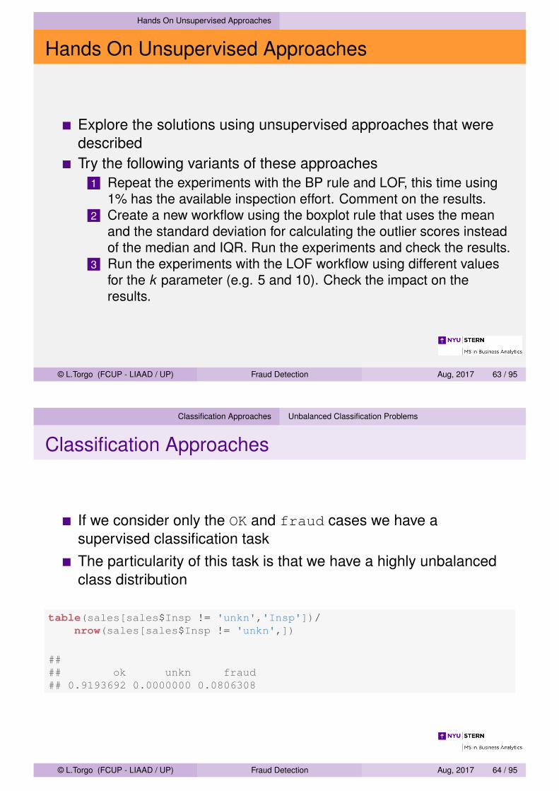
Hands On Unsupervised Approaches
Explore the solutions using unsupervised approaches that weredescribedTry the following variants of these approaches
1 Repeat the experiments with the BP rule and LOF, this time using1% has the available inspection effort. Comment on the results.
2 Create a new workflow using the boxplot rule that uses the meanand the standard deviation for calculating the outlier scores insteadof the median and IQR. Run the experiments and check the results.
3 Run the experiments with the LOF workflow using different valuesfor the k parameter (e.g. 5 and 10). Check the impact on theresults.
© L.Torgo (FCUP - LIAAD / UP) Fraud Detection Aug, 2017 63 / 95
Classification Approaches Unbalanced Classification Problems
Classification Approaches
If we consider only the OK and fraud cases we have asupervised classification taskThe particularity of this task is that we have a highly unbalancedclass distribution
table(sales[sales$Insp != 'unkn','Insp'])/nrow(sales[sales$Insp != 'unkn',])
#### ok unkn fraud## 0.9193692 0.0000000 0.0806308
© L.Torgo (FCUP - LIAAD / UP) Fraud Detection Aug, 2017 64 / 95
Classification Approaches Unbalanced Classification Problems
Classification Approaches (2)
This type of problems creates serious difficulties to mostclassification algorithmsThey will tend to focus on the prevailing class valueThe problem is that this class is the least important on thisapplication !The are essentially 2 ways of addressing these problems
1 Change the learning algorithms, namely their preference biascriteria
2 Change the distribution of the data to balance it
© L.Torgo (FCUP - LIAAD / UP) Fraud Detection Aug, 2017 65 / 95
Classification Approaches SMOTE
Sampling MethodsSMOTE
Sampling methods change the distribution of the data by samplingover the available data setThe goal is to make the training sample more adequate for ourobjectivesSMOTE is amongst the most successful sampling methods
SMOTE under-samples the majority classSMOTE also over-samples the minority class creating several newcases by clever interpolation on the provided casesThe result is a less unbalanced data set
Package UBL implements several sampling approaches includingSMOTE, through function SmoteClassifThe result of this function is a new (more balanced) data set
Chawla, N. V., Bowyer, K. W., Hall, L. O., and Kegelmeyer, W. P. (2002). Smote: Synthetic minority over-sampling technique. JAIR,16:321-357.P. Branco, L. Torgo and R. Ribeiro (2016). A Survey of Predictive Modeling on Imbalanced Domains. ACM Computing Surveys, 49 (2),31.
P. Branco, R. Ribeiro and L. Torgo (2016). A UBL: an R package for Utility-based Learning. CoRR abs/1604.08079.
© L.Torgo (FCUP - LIAAD / UP) Fraud Detection Aug, 2017 66 / 95
Classification Approaches The Naive Bayes Classification Algorithm
Bayesian Classification
Bayesian classifiers are statistical classifiers - they predict theprobability that a case belongs to a certain classBayesian classification is based on the Bayes Theorem (nextslide)A particular class of Bayesian classifiers - the Naive BayesClassifier - has shown rather competitive performance on severalproblems even when compared to more “sophisticated” methodsNaive Bayes is available in R on package e1071, through functionnaiveBayes()
© L.Torgo (FCUP - LIAAD / UP) Fraud Detection Aug, 2017 67 / 95
Classification Approaches The Naive Bayes Classification Algorithm
The Bayes Theorem (1)
Let D be a data set formed by n cases {〈x, y〉}ni=1, where x is avector of p variable values and y is the value on a target nominalvariable Y ∈ YLet H be a hypothesis that states that a certain test cases belongsto a class c ∈ YGiven a new test case x the goal of classification is to estimateP(H|x), i.e. the probability that H holds given the evidence xMore specifically, if Y is the domain of the target variable Y wewant to estimate the probability of each of the possible valuesgiven the test case (evidence) x
© L.Torgo (FCUP - LIAAD / UP) Fraud Detection Aug, 2017 68 / 95
Classification Approaches The Naive Bayes Classification Algorithm
The Bayes Theorem (2)
P(H|x) is called the posterior probability, or a posterioriprobability, of H conditioned on xWe can also talk about P(H), the prior probability, or a prioriprobability, of the hypothesis HNotice that P(H|x) is based on more information than P(H), whichis independent of the observation xFinally, we can also talk about P(x|H) as the posterior probabilityof x conditioned on H
Bayes’ Theorem
P(H|x) = P(x|H)P(H)
P(x)
© L.Torgo (FCUP - LIAAD / UP) Fraud Detection Aug, 2017 69 / 95
Classification Approaches The Naive Bayes Classification Algorithm
The Naive Bayes Classifier
How it works?
We have a data set D with cases belonging to one of m classesc1, c2, · · · , cm
Given a new test case x this classifier produces as prediction theclass that has the highest estimated probability, i.e.maxi∈{1,2,··· ,m} P(ci |x)Given that P(x) is constant for all classes, according to the BayesTheorem the class with the highest probability is the onemaximizing the quantity P(x|ci)P(ci)
© L.Torgo (FCUP - LIAAD / UP) Fraud Detection Aug, 2017 70 / 95
Classification Approaches The Naive Bayes Classification Algorithm
The Naive Bayes Classifier (2)
How it works? (cont.)
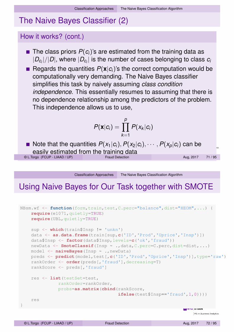
The class priors P(ci)’s are estimated from the training data as|Dci |/|D|, where |Dci | is the number of cases belonging to class ci
Regards the quantities P(x|ci)’s the correct computation would becomputationally very demanding. The Naive Bayes classifiersimplifies this task by naively assuming class conditionindependence. This essentially resumes to assuming that there isno dependence relationship among the predictors of the problem.This independence allows us to use,
P(x|ci) =
p∏k=1
P(xk |ci)
Note that the quantities P(x1|ci),P(x2|ci), · · · ,P(xp|ci) can beeasily estimated from the training data
© L.Torgo (FCUP - LIAAD / UP) Fraud Detection Aug, 2017 71 / 95
Classification Approaches The Naive Bayes Classification Algorithm
Using Naive Bayes for Our Task together with SMOTE
NBsm.wf <- function(form,train,test,C.perc="balance",dist="HEOM",...) {require(e1071,quietly=TRUE)require(UBL,quietly=TRUE)
sup <- which(train$Insp != 'unkn')data <- as.data.frame(train[sup,c('ID','Prod','Uprice','Insp')])data$Insp <- factor(data$Insp,levels=c('ok','fraud'))newData <- SmoteClassif(Insp ~ .,data,C.perc=C.perc,dist=dist,...)model <- naiveBayes(Insp ~ .,newData)preds <- predict(model,test[,c('ID','Prod','Uprice','Insp')],type='raw')rankOrder <- order(preds[,'fraud'],decreasing=T)rankScore <- preds[,'fraud']
res <- list(testSet=test,rankOrder=rankOrder,probs=as.matrix(cbind(rankScore,
ifelse(test$Insp=='fraud',1,0))))res
}
© L.Torgo (FCUP - LIAAD / UP) Fraud Detection Aug, 2017 72 / 95
Classification Approaches The Naive Bayes Classification Algorithm
Evaluating the Naive Bayes model
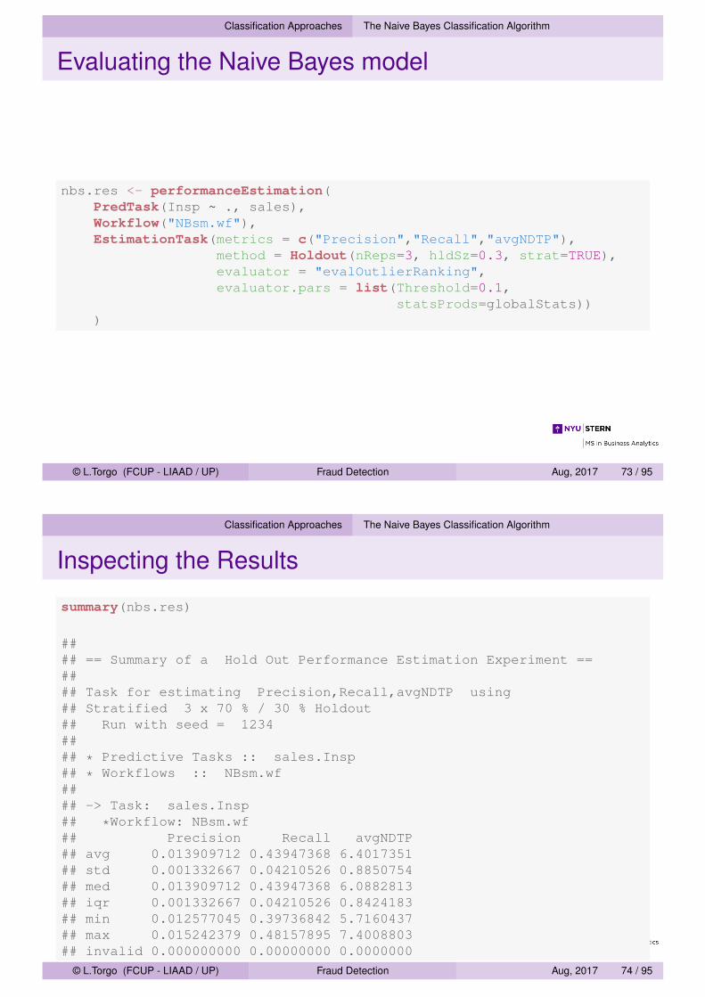
nbs.res <- performanceEstimation(PredTask(Insp ~ ., sales),Workflow("NBsm.wf"),EstimationTask(metrics = c("Precision","Recall","avgNDTP"),
method = Holdout(nReps=3, hldSz=0.3, strat=TRUE),evaluator = "evalOutlierRanking",evaluator.pars = list(Threshold=0.1,
statsProds=globalStats)))
© L.Torgo (FCUP - LIAAD / UP) Fraud Detection Aug, 2017 73 / 95
Classification Approaches The Naive Bayes Classification Algorithm
Inspecting the Results
summary(nbs.res)
#### == Summary of a Hold Out Performance Estimation Experiment ==#### Task for estimating Precision,Recall,avgNDTP using## Stratified 3 x 70 % / 30 % Holdout## Run with seed = 1234#### * Predictive Tasks :: sales.Insp## * Workflows :: NBsm.wf#### -> Task: sales.Insp## *Workflow: NBsm.wf## Precision Recall avgNDTP## avg 0.013909712 0.43947368 6.4017351## std 0.001332667 0.04210526 0.8850754## med 0.013909712 0.43947368 6.0882813## iqr 0.001332667 0.04210526 0.8424183## min 0.012577045 0.39736842 5.7160437## max 0.015242379 0.48157895 7.4008803## invalid 0.000000000 0.00000000 0.0000000
© L.Torgo (FCUP - LIAAD / UP) Fraud Detection Aug, 2017 74 / 95
Classification Approaches The Naive Bayes Classification Algorithm
Performance for Different Effort Levels
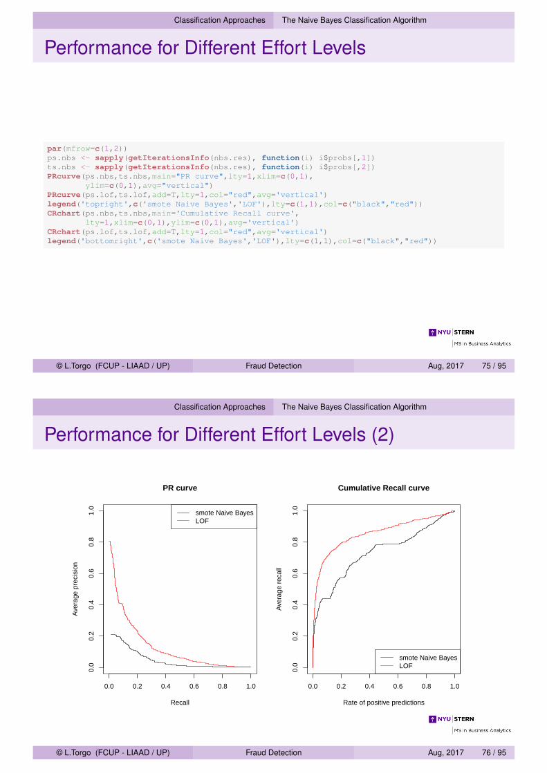
par(mfrow=c(1,2))ps.nbs <- sapply(getIterationsInfo(nbs.res), function(i) i$probs[,1])ts.nbs <- sapply(getIterationsInfo(nbs.res), function(i) i$probs[,2])PRcurve(ps.nbs,ts.nbs,main="PR curve",lty=1,xlim=c(0,1),
ylim=c(0,1),avg="vertical")PRcurve(ps.lof,ts.lof,add=T,lty=1,col="red",avg='vertical')legend('topright',c('smote Naive Bayes','LOF'),lty=c(1,1),col=c("black","red"))CRchart(ps.nbs,ts.nbs,main='Cumulative Recall curve',
lty=1,xlim=c(0,1),ylim=c(0,1),avg='vertical')CRchart(ps.lof,ts.lof,add=T,lty=1,col="red",avg='vertical')legend('bottomright',c('smote Naive Bayes','LOF'),lty=c(1,1),col=c("black","red"))
© L.Torgo (FCUP - LIAAD / UP) Fraud Detection Aug, 2017 75 / 95
Classification Approaches The Naive Bayes Classification Algorithm
Performance for Different Effort Levels (2)
PR curve
Recall
Ave
rage
pre
cisi
on
0.0 0.2 0.4 0.6 0.8 1.0
0.0
0.2
0.4
0.6
0.8
1.0
smote Naive BayesLOF
Cumulative Recall curve
Rate of positive predictions
Ave
rage
rec
all
0.0 0.2 0.4 0.6 0.8 1.0
0.0
0.2
0.4
0.6
0.8
1.0
smote Naive BayesLOF
© L.Torgo (FCUP - LIAAD / UP) Fraud Detection Aug, 2017 76 / 95

Classification Approaches The AdaBoost Algorithm
The AdaBoost Algorithm
The AdaBoost method is a boosting algorithm that belongs to theclass of Ensemble methodsBoosting was developed with the goal of answering the question:Can a set of weak learners create a single strong learner?In the above question a “weak” learner is a model that alone hasvery poor predictive performance
Rob Schapire (1990). Strength of Weak Learnability. Machine Learning Vol. 5, pages197–227.
© L.Torgo (FCUP - LIAAD / UP) Fraud Detection Aug, 2017 77 / 95
Classification Approaches The AdaBoost Algorithm
The AdaBoost Algorithm (2)
Boosting algorithms work by iteratively creating a strong learner byadding at each iteration a new weak learner to make the ensembleWeak learners are added with weights that reflect the learner’saccuracyAfter each addition the data is re-weighted such that cases thatare still poorly predicted gain more weight for the next iterationThis means that each new weak learner will focus on the errors ofthe previous ones
Rob Schapire (1990). Strength of Weak Learnability. Machine Learning Vol. 5, pages197–227.
© L.Torgo (FCUP - LIAAD / UP) Fraud Detection Aug, 2017 78 / 95
Classification Approaches The AdaBoost Algorithm
The AdaBoost Algorithm (3)
AdaBoost (Adaptive Boosting) is an ensemble algorithm that canbe used to improve the performance of a base algorithmIt consists of an iterative process where new models are added toform an ensembleIt is adaptive in the sense that at each new iteration of thealgorithm the new models are built to try to overcome the errorsmade in the previous iterationsAt each iteration the weights of the training cases are adjusted sothat cases that were wrongly predicted get their weight increasedto make new models focus on accurately predicting themAdaBoost was created for classification although variants forregression exist
Y. Freund and R. Schapire (1996). Experiments with a new boosting algorithm, inProc. of 13th International Conference on Machine Learning
© L.Torgo (FCUP - LIAAD / UP) Fraud Detection Aug, 2017 79 / 95
Classification Approaches The AdaBoost Algorithm
The AdaBoost Algorithm
The goal of the algorithm is to reach a form of additive modelcomposed of k weak models
H(xi) =∑
k
wkhk (xi)
where wk is the weight of the weak model hk (xi)
All training cases start with a weight equal to d1(xi) = 1/n, wheren is the training set size
© L.Torgo (FCUP - LIAAD / UP) Fraud Detection Aug, 2017 80 / 95

Classification Approaches The AdaBoost Algorithm
The AdaBoost Algorithm
AdaBoost is available in several R packagesThe package adabag is an example with the functionboosting()
The packages gbm and xgboost include implementations ofboosting for regression tasksWe will use the package RWeka that provides the functionAdaBoost.M1()
© L.Torgo (FCUP - LIAAD / UP) Fraud Detection Aug, 2017 81 / 95
Classification Approaches The AdaBoost Algorithm
Using AdaBoost for Our Task
ab.wf <- function(form,train,test,ntrees=100,...) {require(RWeka,quietly=TRUE)sup <- which(train$Insp != 'unkn')data <- as.data.frame(train[sup,c('ID','Prod','Uprice','Insp')])data$Insp <- factor(data$Insp,levels=c('ok','fraud'))model <- AdaBoostM1(Insp ~ .,data,
control=Weka_control(I=ntrees))preds <- predict(model,test[,c('ID','Prod','Uprice','Insp')],
type='probability')rankOrder <- order(preds[,"fraud"],decreasing=TRUE)rankScore <- preds[,"fraud"]
res <- list(testSet=test,rankOrder=rankOrder,probs=as.matrix(cbind(rankScore,
ifelse(test$Insp=='fraud',1,0))))res
}
© L.Torgo (FCUP - LIAAD / UP) Fraud Detection Aug, 2017 82 / 95
Classification Approaches The AdaBoost Algorithm
Evaluating the AdaBoost model
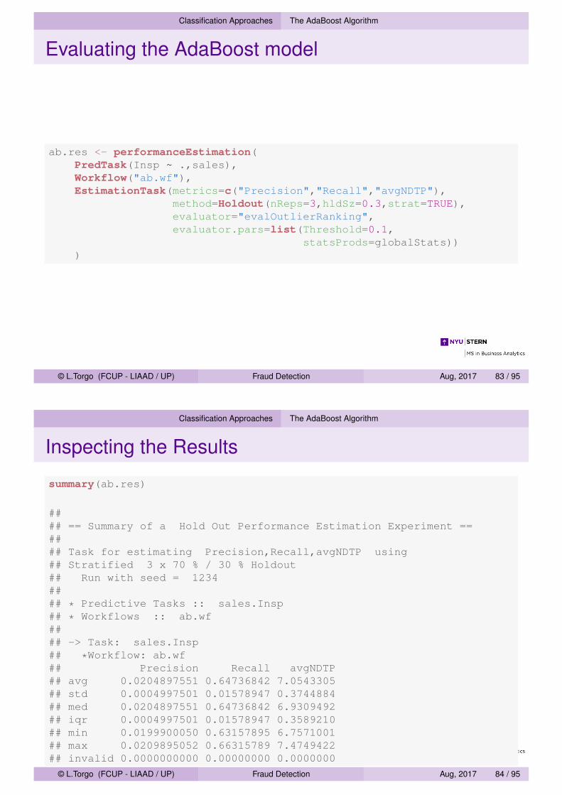
ab.res <- performanceEstimation(PredTask(Insp ~ .,sales),Workflow("ab.wf"),EstimationTask(metrics=c("Precision","Recall","avgNDTP"),
method=Holdout(nReps=3,hldSz=0.3,strat=TRUE),evaluator="evalOutlierRanking",evaluator.pars=list(Threshold=0.1,
statsProds=globalStats)))
© L.Torgo (FCUP - LIAAD / UP) Fraud Detection Aug, 2017 83 / 95
Classification Approaches The AdaBoost Algorithm
Inspecting the Results
summary(ab.res)
#### == Summary of a Hold Out Performance Estimation Experiment ==#### Task for estimating Precision,Recall,avgNDTP using## Stratified 3 x 70 % / 30 % Holdout## Run with seed = 1234#### * Predictive Tasks :: sales.Insp## * Workflows :: ab.wf#### -> Task: sales.Insp## *Workflow: ab.wf## Precision Recall avgNDTP## avg 0.0204897551 0.64736842 7.0543305## std 0.0004997501 0.01578947 0.3744884## med 0.0204897551 0.64736842 6.9309492## iqr 0.0004997501 0.01578947 0.3589210## min 0.0199900050 0.63157895 6.7571001## max 0.0209895052 0.66315789 7.4749422## invalid 0.0000000000 0.00000000 0.0000000
© L.Torgo (FCUP - LIAAD / UP) Fraud Detection Aug, 2017 84 / 95
Classification Approaches The AdaBoost Algorithm
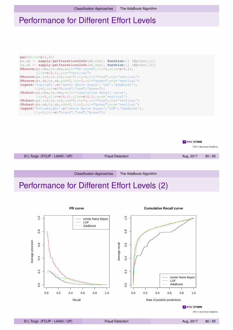
Performance for Different Effort Levels
par(mfrow=c(1,2))ps.ab <- sapply(getIterationsInfo(ab.res), function(i) i$probs[,1])ts.ab <- sapply(getIterationsInfo(ab.res), function(i) i$probs[,2])PRcurve(ps.nbs,ts.nbs,main="PR curve",lty=1,xlim=c(0,1),
ylim=c(0,1),avg="vertical")PRcurve(ps.lof,ts.lof,add=T,lty=1,col="red",avg='vertical')PRcurve(ps.ab,ts.ab,add=T,lty=1,col="green",avg='vertical')legend('topright',c('smote Naive Bayes','LOF','AdaBoost'),
lty=1,col=c("black","red","green"))CRchart(ps.nbs,ts.nbs,main='Cumulative Recall curve',
lty=1,xlim=c(0,1),ylim=c(0,1),avg='vertical')CRchart(ps.lof,ts.lof,add=T,lty=1,col="red",avg='vertical')CRchart(ps.ab,ts.ab,add=T,lty=1,col="green",avg='vertical')legend('bottomright',c('smote Naive Bayes','LOF','AdaBoost'),
lty=1,col=c("black","red","green"))
© L.Torgo (FCUP - LIAAD / UP) Fraud Detection Aug, 2017 85 / 95
Classification Approaches The AdaBoost Algorithm
Performance for Different Effort Levels (2)
PR curve
Recall
Ave
rage
pre
cisi
on
0.0 0.2 0.4 0.6 0.8 1.0
0.0
0.2
0.4
0.6
0.8
1.0
smote Naive BayesLOFAdaBoost
Cumulative Recall curve
Rate of positive predictions
Ave
rage
rec
all
0.0 0.2 0.4 0.6 0.8 1.0
0.0
0.2
0.4
0.6
0.8
1.0
smote Naive BayesLOFAdaBoost
© L.Torgo (FCUP - LIAAD / UP) Fraud Detection Aug, 2017 86 / 95
Hands On Classification Approaches
Hands On Classification Approaches
Explore the solutions using classification approaches that weredescribedTry the following variants of these approaches
1 The workflow using Naive Bayes generates a more balanceddistribution through SMOTE. Explore different settings of SMOTEand check the impact on the results. Suggestion: check the helppage of the function SmoteClassif()
2 Modify the Naive Bayes workflow to completely eliminate SMOTE,i.e. use the original unbalanced data. Check and comment on theresults.
3 Change the number of trees used in the ensemble obtained withthe adaboost workflow. Check the results. Tip: try a large number!
© L.Torgo (FCUP - LIAAD / UP) Fraud Detection Aug, 2017 87 / 95
Semi-supervised Approaches
Semi-Supervised ApproachesSelf Training
Self training is a generic semi-supervised method that can beapplied to any classification methodIt is an iterative process consisting of the following main steps:
1 Build a classifier with the current labeled data2 Use the model to classify the unlabeled data3 Select the highest confidence classifications and add the respective
cases with that classification to the labeled data4 Repeat the process until some criteria are met
The last classifier of this iterative process is the result of thesemi-supervised processFunction SelfTrain() on package DMwR2 implements theseideas for any probabilistic classifier
© L.Torgo (FCUP - LIAAD / UP) Fraud Detection Aug, 2017 88 / 95
Semi-supervised Approaches
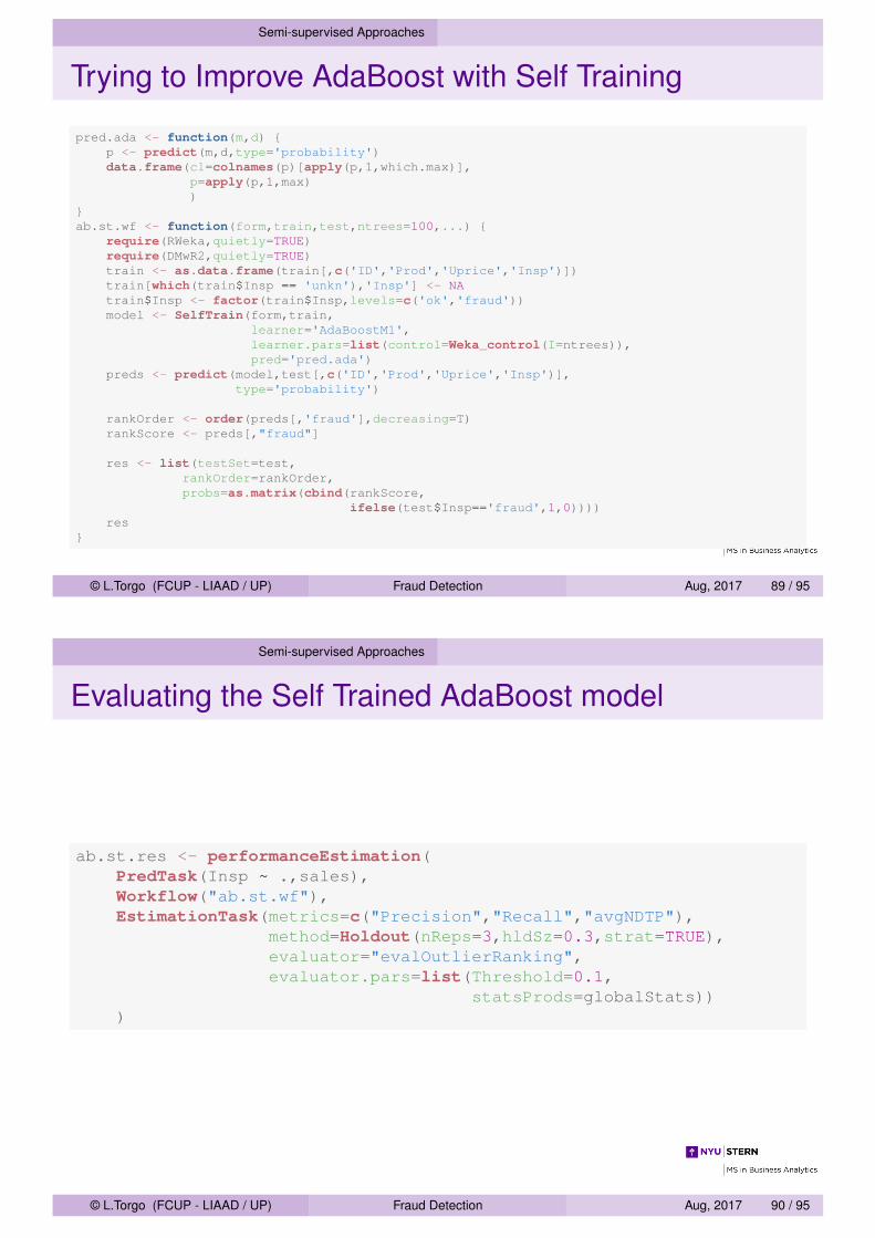
Trying to Improve AdaBoost with Self Training
pred.ada <- function(m,d) {p <- predict(m,d,type='probability')data.frame(cl=colnames(p)[apply(p,1,which.max)],
p=apply(p,1,max))
}ab.st.wf <- function(form,train,test,ntrees=100,...) {
require(RWeka,quietly=TRUE)require(DMwR2,quietly=TRUE)train <- as.data.frame(train[,c('ID','Prod','Uprice','Insp')])train[which(train$Insp == 'unkn'),'Insp'] <- NAtrain$Insp <- factor(train$Insp,levels=c('ok','fraud'))model <- SelfTrain(form,train,
learner='AdaBoostM1',learner.pars=list(control=Weka_control(I=ntrees)),pred='pred.ada')
preds <- predict(model,test[,c('ID','Prod','Uprice','Insp')],type='probability')
rankOrder <- order(preds[,'fraud'],decreasing=T)rankScore <- preds[,"fraud"]
res <- list(testSet=test,rankOrder=rankOrder,probs=as.matrix(cbind(rankScore,
ifelse(test$Insp=='fraud',1,0))))res
}
© L.Torgo (FCUP - LIAAD / UP) Fraud Detection Aug, 2017 89 / 95
Semi-supervised Approaches
Evaluating the Self Trained AdaBoost model
ab.st.res <- performanceEstimation(PredTask(Insp ~ .,sales),Workflow("ab.st.wf"),EstimationTask(metrics=c("Precision","Recall","avgNDTP"),
method=Holdout(nReps=3,hldSz=0.3,strat=TRUE),evaluator="evalOutlierRanking",evaluator.pars=list(Threshold=0.1,
statsProds=globalStats)))
© L.Torgo (FCUP - LIAAD / UP) Fraud Detection Aug, 2017 90 / 95
Semi-supervised Approaches
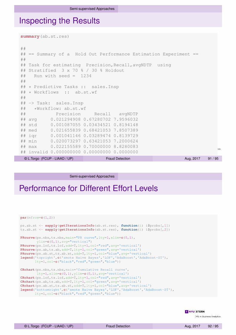
Inspecting the Results
summary(ab.st.res)
#### == Summary of a Hold Out Performance Estimation Experiment ==#### Task for estimating Precision,Recall,avgNDTP using## Stratified 3 x 70 % / 30 % Holdout## Run with seed = 1234#### * Predictive Tasks :: sales.Insp## * Workflows :: ab.st.wf#### -> Task: sales.Insp## *Workflow: ab.st.wf## Precision Recall avgNDTP## avg 0.021294908 0.67280702 7.9596032## std 0.001087055 0.03434521 0.8194148## med 0.021655839 0.68421053 7.8507389## iqr 0.001041146 0.03289474 0.8139729## min 0.020073297 0.63421053 7.2000624## max 0.022155589 0.70000000 8.8280083## invalid 0.000000000 0.00000000 0.0000000
© L.Torgo (FCUP - LIAAD / UP) Fraud Detection Aug, 2017 91 / 95
Semi-supervised Approaches
Performance for Different Effort Levels
par(mfrow=c(1,2))
ps.ab.st <- sapply(getIterationsInfo(ab.st.res), function(i) i$probs[,1])ts.ab.st <- sapply(getIterationsInfo(ab.st.res), function(i) i$probs[,2])
PRcurve(ps.nbs,ts.nbs,main="PR curve",lty=1,xlim=c(0,1),ylim=c(0,1),avg="vertical")
PRcurve(ps.lof,ts.lof,add=T,lty=1,col="red",avg='vertical')PRcurve(ps.ab,ts.ab,add=T,lty=1,col="green",avg='vertical')PRcurve(ps.ab.st,ts.ab.st,add=T,lty=1,col="blue",avg='vertical')legend('topright',c('smote Naive Bayes','LOF','AdaBoost','AdaBoost-ST'),
lty=1,col=c("black","red","green","blue"))
CRchart(ps.nbs,ts.nbs,main='Cumulative Recall curve',lty=1,xlim=c(0,1),ylim=c(0,1),avg='vertical')
CRchart(ps.lof,ts.lof,add=T,lty=1,col="red",avg='vertical')CRchart(ps.ab,ts.ab,add=T,lty=1,col="green",avg='vertical')CRchart(ps.ab.st,ts.ab.st,add=T,lty=1,col="blue",avg='vertical')legend('bottomright',c('smote Naive Bayes','LOF','AdaBoost','AdaBoost-ST'),
lty=1,col=c("black","red","green","blue"))
© L.Torgo (FCUP - LIAAD / UP) Fraud Detection Aug, 2017 92 / 95
Semi-supervised Approaches
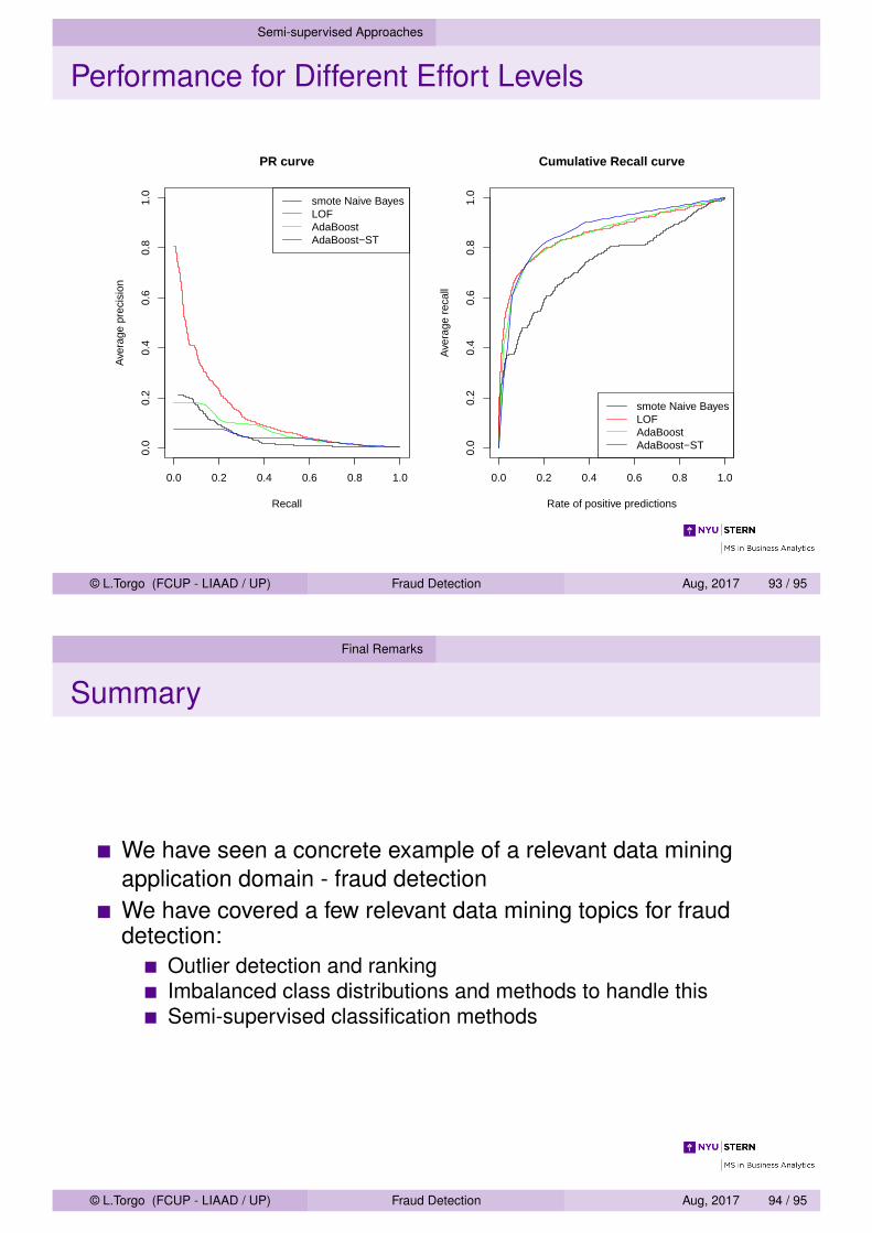
Performance for Different Effort Levels
PR curve
Recall
Ave
rage
pre
cisi
on
0.0 0.2 0.4 0.6 0.8 1.0
0.0
0.2
0.4
0.6
0.8
1.0
smote Naive BayesLOFAdaBoostAdaBoost−ST
Cumulative Recall curve
Rate of positive predictions
Ave
rage
rec
all
0.0 0.2 0.4 0.6 0.8 1.00.
00.
20.
40.
60.
81.
0
smote Naive BayesLOFAdaBoostAdaBoost−ST
© L.Torgo (FCUP - LIAAD / UP) Fraud Detection Aug, 2017 93 / 95
Final Remarks
Summary
We have seen a concrete example of a relevant data miningapplication domain - fraud detectionWe have covered a few relevant data mining topics for frauddetection:
Outlier detection and rankingImbalanced class distributions and methods to handle thisSemi-supervised classification methods
© L.Torgo (FCUP - LIAAD / UP) Fraud Detection Aug, 2017 94 / 95

Hands On Semi-Supervised Approaches
Hands On Semi-Supervised Approaches
Explore the solutions using the self trained AdaBoost modelTry the following variants
1 Explore the help page of function SelfTrain() and try differentsettings on the workflow of AdaBoost
© L.Torgo (FCUP - LIAAD / UP) Fraud Detection Aug, 2017 95 / 95