A Collection of Exercises in Advanced Probability …josic/old_website/myweb/teaching...Hence, Pis the desired probability measure, proving the su ciency. Exercise 1.3.4. Suppose that

A Collection of Exercisesin

Advanced Probability Theory

The Solutions Manualof

All Even-Numbered Exercisesfrom

“A First Look at Rigorous Probability Theory”(Second Edition, 2006)

Mohsen SoltanifarUniversity of Saskatchewan, Canada

[email protected]

Longhai LiUniversity of Saskatchewan, Canada

[email protected]

Jeffrey S. RosenthalUniversity of Toronto, Canada

[email protected]

(July 17, 2010.)

Copyright c© 2010 by World Scientific Publishing Co. Pte. Ltd.

ii

Published by

World Scientific Publishing Co. Pte. Ltd.5 Toh Tuck Link, Singapor 596224

USA office: 27 Warren Street, Suite 401-402, Hackensack, NJ 07601

UK office: 57 Shelton Street, Covent Garden, London WC2H 9HE

Web site: www.WorldScientific.com

A Collection of Exercises in Advanced Probability Theory

Copyright c© 2010 by World Scientific Publishing Co. Pte. Ltd.

Preface

I am very pleased that, thanks to the hard work of Mohsen Soltanifar and Longhai Li, this solutionsmanual for my book1 is now available. I hope readers will find these solutions helpful as you strugglewith learning the foundations of measure-theoretic probability. Of course, you will learn best if youfirst attempt to solve the exercises on your own, and only consult this manual when you are reallystuck (or to check your solution after you think you have it right).

For course instructors, I hope that these solutions will assist you in teaching students, by offeringthem some extra guidance and information.

My book has been widely used for self-study, in addition to its use as a course textbook, allowing avariety of students and professionals to learn the foundations of measure-theoretic probability theoryon their own time. Many self-study students have written to me requesting solutions to help assesstheir progress, so I am pleased that this manual will fill that need as well.

Solutions manuals always present a dilemma: providing solutions can be very helpful to studentsand self-studiers, but make it difficult for course instructors to assign exercises from the book for coursecredit. To balance these competing demands, we considered maintaining a confidential “instructorsand self-study students only” solutions manual, but decided that would be problematic and ultimatelyinfeasible. Instead, we settled on the compromise of providing a publicly-available solutions manual,but to even-numbered exercises only. In this way, it is hoped that readers can use the even-numberedexercise solutions to learn and assess their progress, while instructors can still assign odd-numberedexercises for course credit as desired.

Of course, this solutions manual may well contain errors, perhaps significant ones. If you find some,then please e-mail me and I will try to correct them promptly. (I also maintain an errata list for thebook itself, on my web site, and will add book corrections there.)

Happy studying!

Jeffrey S. RosenthalToronto, Canada, 2010

[email protected]

http://probability.ca/jeff/

1J.S. Rosenthal, A First Look at Rigourous Probability Theory, 2nd ed. World Scientific Publishing, Singapore, 2006.219 pages. ISBN: 981-270-371-5 / 981-270-371-3 (paperback).

iv

Contents

1 The need for measure theory 1

2 Probability triples 3

3 Further probabilistic foundations 9

4 Expected values 15

5 Inequalities and convergence 21

6 Distributions of random variables 25

7 Stochastic processes and gambling games 29

8 Discrete Markov chains 33

9 More probability theorems 41

10 Weak convergence 45

11 Characteristic functions 51

12 Decompositions of probability laws 55

13 Conditional probability and expectation 59

14 Martingales 63

15 General stochastic processes 71

vi

Chapter 1

The need for measure theory

Exercise 1.3.2. Suppose Ω = 1, 2, 3 and F is a collection of all subsets of Ω. Find (with proof)necessary and sufficient conditions on the real numbers x, y, and z such that there exists a countablyadditive probability measure P on F , with x = P1, 2, y = P2, 3, and z = P1, 3.

Solution. The necessary and sufficient conditions are: 0 ≤ x ≤ 1, 0 ≤ y ≤ 1, 0 ≤ z ≤ 1, andx+ y + z = 2.

To prove necessity, let P be a probability measure on Ω. Then, for

x = P1, 2 = P1+ P2,

y = P2, 3 = P2+ P3,

and

z = P1, 3 = P1+ P3

we have by definition that 0 ≤ x ≤ 1, 0 ≤ y ≤ 1, and 0 ≤ z ≤ 1, and furthermore we compute that

x+ y + z = 2(P1+ P2+ P3) = 2P (Ω) = 2,

thus proving the necessity.

Conversely, assume that 0 ≤ x ≤ 1, 0 ≤ y ≤ 1, 0 ≤ z ≤ 1, and x + y + z = 2. Then, define thedesired countably additive probability measure P as follows:

P (φ) = 0,

P1 = 1− y,P2 = 1− z,P3 = 1− x,

P1, 2 = x,

P1, 3 = z,

P2, 3 = y,

P1, 2, 3 = 1.

2 Chapter 1: The need for measure theory

It is easily checked directly that for any two disjoint sets A,B ⊆ Ω, we have

P (A ∪B) = P (A) + P (B)

For example, if A = 1 and B = 2, then since x + y + z = 2, P (A ∪ B) = P1, 2 = x whileP (A) + P (B) = P1+ P2 = (1− y) + (1− z) = 2− y − z = (x+ y + z)− y − z = x = P (A ∪B).Hence, P is the desired probability measure, proving the sufficiency.

Exercise 1.3.4. Suppose that Ω = N, and P is defined for all A ⊆ Ω by P (A) = |A| if A is finite(where |A| is the number of elements in the subset A), and P (A) = ∞ if A is infinite. This P is ofcourse not a probability measure(in fact it is counting measure), however we can still ask the following.(By convention, ∞+∞ =∞.)(a) Is P finitely additive?(b) Is P countably additive?

Solution.(a) Yes. Let A,B ⊆ Ω be disjoint. We consider two different cases.

Case 1: At least one of A or B is infinite. Then A ∪ B is infinite. Consequently, P (A ∪ B) and atleast one of P (A) or P (B) will be infinite. Hence, P (A ∪ B) = ∞ and P (A) + P (B) = ∞, implyingP (A ∪B) =∞ = P (A) + P (B).

Case 2: Both of A and B are finite. Then P (A ∪B) = |A ∪B| = |A|+ |B| = P (A) + P (B).

Accordingly, P is finitely additive.

(b) Yes. Let A1, A2, · · · be a sequence of disjoint subsets of Ω. We consider two different cases.

Case 1: At least one of An’s is infinite. Then ∪∞n=1An is infinite. Consequently, P (∪∞n=1An) andat least one of P (An)’s will be infinite. Hence, P (∪∞n=1An) = ∞ and

∑∞n=1 P (An) = ∞, implying

P (∪∞n=1An) =∞ =∑∞

n=1 P (An).

Case 2: All of An’s are finite. Then depending on finiteness of ∪∞n=1An we consider two cases. First,let ∪∞n=1An be infinite, then, P (∪∞n=1An) = ∞ =

∑∞n=1 |An| =

∑∞n=1 P (An). Second, let ∪∞n=1An be

finite, then,

P (∪∞n=1An) = | ∪∞n=1 An| =∞∑n=1

|An| =∞∑n=1

P (An).

Accordingly, P is countably additive.

Chapter 2

Probability triples

Exercise 2.7.2. Let Ω = 1, 2, 3, 4, and let J = 1, 2. Describe explicitly the σ-algebra σ(J )generated by J .

Solution.

σ(J ) = φ, 1, 2, 1, 2, 3, 4, 1, 3, 4, 2, 3, 4,Ω.

Exercise 2.7.4. Let F1,F2, · · · be a sequence of collections of subsets of Ω, such that Fn ⊆ Fn+1 foreach n.(a) Suppose that each Fi is an algebra. Prove that ∪∞i=1Fiis also an algebra.(b) Suppose that each Fi is a σ-algebra. Show (by counterexample) that ∪∞i=1Fi might not be a σ-algebra.

Solution.(a) First, since φ,Ω ∈ F1 andF1 ⊆ ∪∞i=1Fi, we have φ,Ω ∈ ∪∞i=1Fi. Second, let A ∈ ∪∞i=1Fi,then A ∈ Fi for some i. On the other hand, Ac ∈ Fi and Fi ⊆ ∪∞i=1Fi, implying Ac ∈ ∪∞i=1Fi.Third, let A,B ∈ ∪∞i=1Fi, then A ∈ Fi and B ∈ Fj , for some i, j. However, A,B ∈ Fmax(i,j) yieldingA ∪B ∈ Fmax(i,j). On the other had, Fmax(i,j) ⊆ ∪∞i=1Fi implying A ∪B ∈ ∪∞i=1Fi.

(b) Put Ωi = jij=1, and let Fi be the σ-algebra of the collection of all subsets of Ωi for i ∈ N. Supposethat ∪∞i=1Fi is also a σ-algebra. Since, for each i, i ∈ Fi and Fi ⊆ ∪∞i=1Fi we have i ∈ ∪∞i=1Fi.Thus, by our primary assumption, N = ∪∞i=1i ∈ ∪∞i=1Fi and, therefore, N ∈ Fi for some i, whichimplies N ⊆ Ωi , a contradiction. Hence, ∪∞i=1Fi is not a σ-algebra.

Exercise 2.7.6. Suppose that Ω = [0, 1] is the unit interval, and F is the set of all subsets A suchthat either A or Ac is finite, and P is defined by P (A) = 0 if A is finite, and P (A) = 1 if Ac is finite.(a) Is F an algebra?(b) Is F a σ-algebra?(c) Is P finitely additive?(d) Is P countably additive on F (as the previous exercise)?

4 Chapter 2: Probability triples

Solution. (a) Yes. First, since φ is finite and Ωc = φ is finite, we have φ,Ω ∈ F . Second, let A ∈ F ,then either A or Ac is finite implying either Ac or A is finite, hence, Ac ∈ F . Third, let A,B ∈ F .Then, we have several cases:(i) A finite (Ac infinite):(i-i) B finite (Bc infinite): A ∪B finite , (A ∪B)c = Ac ∩Bc infinite(i-ii) Bc finite (B infinite): A ∪B infinite , (A ∪B)c = Ac ∩Bc finite(ii) Ac finite (A infinite):(ii-i) B finite (Bc infinite): A ∪B infinite , (A ∪B)c = Ac ∩Bc finite(ii-ii) Bc finite (B infinite): A ∪B infinite , (A ∪B)c = Ac ∩Bc finite.Hence, A ∪B ∈ F .

(b) No. For any n ∈ N, 1n ∈ F . But, 1n∞n=1 /∈ F .

(c) Yes. let A,B ∈ F be disjoint. Then, we have several cases:(i) A finite (Ac infinite):(i-i) B finite (Bc infinite): P (A ∪B) = 0 = 0 + 0 = P (A) + P (B)(i-ii) Bc finite (B infinite): P (A ∪B) = 1 = 0 + 1 = P (A) + P (B)(ii) Ac finite (A infinite):(ii-i) B finite (Bc infinite): P (A ∪B) = 1 = 1 + 0 = P (A) + P (B)(ii-ii) Bc finite (B infinite): Since Ac ∪Bc is finite, Ac ∪Bc 6= Ω implying A ∩B 6= φ.Hence, P (A ∪B) = P (A) + P (B).

(d) Yes. Let A1, A2, · · · ∈ F be disjoint such that ∪∞n=1An ∈ F . Then, there are two cases:(i) ∪∞n=1An finite:In this case, for each n ∈ N , An is finite. Therefore, P (∪∞n=1An) = 0 =

∑∞n=1 0 =

∑∞n=1 P (An).

(ii) (∪∞n=1An)c finite ( ∪∞n=1An infinite):In this case, there is some n0 ∈ N such that An0 is infinite.

(In fact, if all An’s are finite, then ∪∞n=1An will be countable. Hence it has Lebesgue measure zeroimplying that its complement has Lebesgue measure one. On the other hand, its complement is finitehaving Lebesgue measure zero, a contradiction.)

Now, let n 6= n0, then An ∩ An0 = φ yields An ⊆ Acn0. But Acn0

is finite, implying that An is finite.Therefore:

P (∪∞n=1An) = 1 = 1 + 0 = P (An0) +∑n6=n0

0 = P (An0) +∑n6=n0

P (An0) =∞∑n=1

P (An).

Accordingly, P is countably additive on F .

Exercise 2.7.8. For the example of Exercise 2.7.7, is P uncountably additive (cf. page 2)?

Chapter 2: Probability triples 5

Solution. No, if it is uncountably additive, then:

1 = P ([0, 1]) = P (∪x∈[0,1]x) =∑x∈[0,1]

P (x) =∑x∈[0,1]

0 = 0,

a contradiction.

Exercise 2.7.10. Prove that the collection J of (2.5.10) is a semi-algebra.

Solution. First, by definition φ,R ∈ J . Second, let A1, A2 ∈ J . If Ai = φ(Ω), then A1 ∩ A2 =φ(Aj) ∈ J . Assume, A1, A2 6= φ,Ω, then we have the following cases:(i) A1 = (−∞, x1]:(i-i) A2 = (−∞, x2]: A1 ∩A2 = (−∞,min(x1, x2)] ∈ J(i-ii) A2 = (y2,∞): A1 ∩A2 = (y2, x1] ∈ J(i-iii) A2 = (x2, y2]: A1 ∩A2 = (x2,min(x1, y2)] ∈ J(ii) A1 = (y1,∞):(ii-i) A2 = (−∞, x2]: A1 ∩A2 = (y1, x2] ∈ J(ii-ii) A2 = (y2,∞): A1 ∩A2 = (max(y1, y2),∞) ∈ J(ii-iii) A2 = (x2, y2]: A1 ∩A2 = (max(x2, y1), y2] ∈ J(iii) A1 = (x1, y1]:(iii-i) A2 = (−∞, x2]: A1 ∩A2 = (x1,min(x2, y1)] ∈ J(iii-ii) A2 = (y2,∞): A1 ∩A2 = (max(y2, x1), y1] ∈ J(iii-iii) A2 = (x2, y2]: A1 ∩A2 = (max(x1, x2),min(y1, y2)] ∈ J .Accordingly, A1 ∩A2 ∈ J . Now, the general case is easily proved by induction (Check!).

Third, let A ∈ J . If A = φ(Ω), then Ac = Ω(φ) ∈ J . If A = (−∞, x], then Ac = (x,∞) ∈ J . IfA = (y,∞), then Ac = (−∞, y] ∈ J . Finally, if A = (x, y], then Ac = (−∞, x] ∪ (y,∞) where bothdisjoint components are in J .

Exercise 2.7.12. Let K be the Cantor set as defined in Subsection 2.4. Let Dn = K⊕ 1n where K⊕ 1

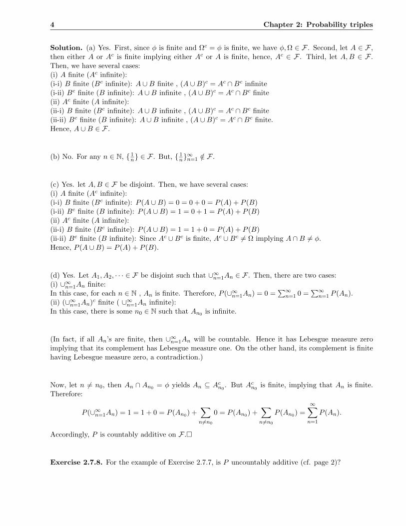
nis defined as in (1.2.4). Let B = ∪∞n=1Dn.(a) Draw a rough sketch of D3.(b) What is λ(D3)?(c) Draw a rough sketch of B.(d) What is λ(B)?

Solution.(a)

Figure 1: Constructing the sketch of the set D3 = K ⊕ 13

(b) λ(D3) = λ(k ⊕ 13) = λ(K) = 0.


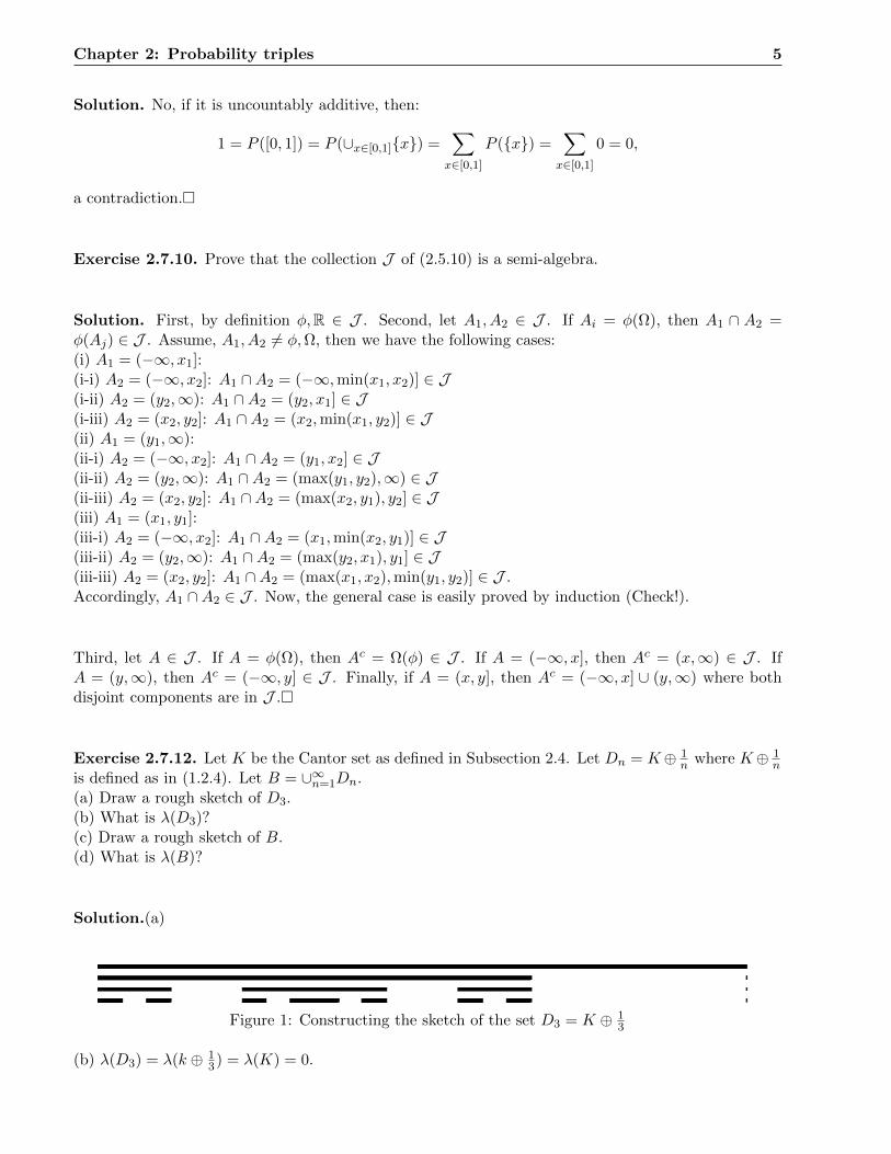
(c)

Figure 2: Constructing the sketch of the set B = ∪∞n=1Dn

In Figure 2, the line one illustrates a rough sketch of the set D1, the line two illustrates a rough sketchof ∪2n=1Dn, the line three illustrates a rough sketch of ∪3n=1Dn, and so on.

(d) From λ(Dn) = λ(k ⊕ 1n) = λ(K) = 0 for all n ∈ N,and λ(B) ≤

∑∞n=1 λ(Dn) it follows that

λ(B) = 0.

Exercise. 2.7.14. Let Ω = 1, 2, 3, 4, with F the collection of all subsets of Ω. Let P and Q betwo probability measures onF , such that P1 = P2 = P3 = P4 = 1

4 , and Q2 = Q4 = 12 ,

extended to F by linearity. Finally, let J = φ,Ω, 1, 2, 2, 3, 3, 4, 1, 4.(a) Prove that P (A) = Q(A) for all A ∈ J .(b) Prove that there is A ∈ σ(J ) with P (A) 6= Q(A).(c) Why does this not contradict Proposition 2.5.8?

Solution. (a)

P (φ) = 0 = Q(φ),

P (Ω) = 1 = Q(Ω),

Pa, b = Pa+ Pb =1

4+

1

4=

1

2= Qa+Qb = Qa, bfor alla 6= b.

(b) Take A = 1, 2, 3 = 1, 2 ∪ 2, 3 ∈ σ(J ). Then:

P (A) =3∑i=1

P (i) =3

46= 1

2=

3∑i=1

Q(i) = Q(A).

(c) Since 1, 2, 2, 3 ∈ J and 1, 2 ∩ 2, 3 = 2 /∈ J , the set J is not a semi-algebra. Thus, thehypothesis of the proposition 2.5.8. is not satisfied by J .

Exercise 2.7.16. (a) Where in the proof of Theorem 2.3.1. was assumption (2.3.3) used?(b) How would the conclusion of Theorem 2.3.1 be modified if assumption (2.3.3) were dropped(butall other assumptions remained the same)?

Solution.(a) It was used in the proof of Lemma 2.3.5.

(b) In the assertion of the Theorem 2.3.1, the equality P ∗(A) = P (A) will be replaced by P ∗(A) ≤ P (A)for all A ∈ J .

Chapter 2: Probability triples 7

Exercise 2.7.18. Let Ω = 1, 2, J = φ,Ω, 1, P (φ) = 0, P (Ω) = 1, and P1 = 13 .

(a) Can Theorem 2.3.1, Corollary 2.5.1, or Corollary 2.5.4 be applied in this case? Why or why not?(b) Can this P be extended to a valid probability measure? Explain.

Solution.(a) No. Because J is not a semi-algebra (in fact 1 ∈ J but 1c = 2 cannot be writtenas a union of disjoint elements of J .

(b) Yes. It is sufficient to put M = φ,Ω, 1, 2 and P †(A) = P (A) if A ∈ J ,23 if A = 2.

Exercise 2.7.20. Let P and Q be two probability measures defined on the same sample space Ω andσ-algebra F .(a) Suppose that P (A) = Q(A) for all A ∈ F with P (A) ≤ 1

2 . Prove that P = Q. i.e. that P (A) = Q(A)for all A ∈ F .(b) Give an example where P (A) = Q(A) for all A ∈ F with P (A) < 1

2 , but such that P 6= Q. i.e. thatP (A) 6= Q(A) for some A ∈ F .

Solution.(a) Let A ∈ F . If P (A) ≤ 12 , then P (A) = Q(A), by assumption. If P (A) > 1

2 , thenP (Ac) < 1

2 . Therefore, 1− P (A) = P (Ac) = Q(Ac) = 1−Q(A) implying P (A) = Q(A).

(b) Take Ω = 1, 2 and F = φ, 1, 2, 1, 2. Define P,Q respectively as follows:

P (φ) = 0, P1 =1

2, P2 =

1

2, andP (Ω) = 1.

Q(φ) = 0, Q1 =1

3, Q2 =

2

3, andP (Ω) = 1.

Exercise 2.7.22. Let (Ω1,F1, P1) be Lebesgue measure on [0, 1]. Consider a second probability triple(Ω2,F2, P2), defined as follows: Ω2 = 1, 2, F2 consists of all subsets of Ω2, and P2 is defined byP21 = 1

3 , P22 = 23 , and additivity. Let (Ω,F , P ) be the product measure of (Ω1,F1, P1) and

(Ω2,F2, P2).(a) Express each of Ω,F , and P as explicitly as possible.(b) Find a set A ∈ F such that P (A) = 3

4 .

Solution.(a) HereF = A× φ,A× 1, A× 2, A× 1, 2 : A ∈ F1.

Then

P (A×B) = 0 if B = φ,λ(A)

3if B = 1, 2λ(A)

3if B = 2, and λ(A) if B = 1, 2.

(b) Take A = [0, 34 ]× 1, 2, then P (A) = λ[0, 34 ] = 3/4.


Chapter 3

Further probabilistic foundations

Exercise 3.6.2. Let (Ω,F , P ) be Lebesgue measure on [0, 1]. Let A = (12 ,34) and B = (0, 23). Are A

and B independent events?

Solution. Yes. In this case, P (A) = 14 , P (B) = 2

3 , and P (A ∩B) = P ((12 ,23)) = 1

6 . Hence:

P (A ∩B) =1

6=

1

4

2

3= P (A)P (B).

Exercise 3.6.4. Suppose An A. Let f : Ω→ R be any function. Prove that limn→∞ infw∈An f(w) =infw∈A f(w).

Solution. Given ε > 0. Using the definition of infimum, there exists wε ∈ A such that f(wε) ≤infw∈A f(w) + ε. On the other hand, A = ∪∞n=1An and An A, therefor, there exists N ∈ N such thatfor any n ∈ N with n ≥ N we have wε ∈ An, implying infw∈An f(w) ≤ f(wε). Combining two recentresults yields:

infw∈An

f(w) < infw∈A

f(w) + ε n = N,N + 1, ....(?)

Next, since AN ⊆ AN+1 ⊆ · · · ⊆ A, for any n ∈ N with n ≥ N we have infw∈A f(w)−ε < infw∈A f(w) ≤infw∈An f(w). Accordingly:

infw∈A

f(w)− ε < infw∈An

f(w) n = N,N + 1, ....(??)

Finally, by (?) and (??):

| infw∈An

f(w)− infw∈A

f(w)| < ε n = N,N + 1, ...,

proving the assertion.

Exercise 3.6.6. Let X,Y, and Z be three independent random variables, and set W = X + Y . Let

10 Chapter 3: Further probabilistic foundations

Bk,n = (n− 1)2−k ≤ X < n2−k and let Ck,m = (m− 1)2−k ≤ Y < m2−k. Let

Ak =⋃

n,m∈Z:(n+m)2−k<x

(Bk,n ∩ Ck,m).

Fix x, z ∈ R, and let A = X + Y < x = W < x and D = Z < z.(a) Prove that Ak A.(b) Prove that Ak and D are independent.(c) By continuity of probabilities, prove that A and D are independent.(d) Use this to prove that W and Z are independent.

Solution.(a) We have:

Ak =⋃

n,m∈Z: (n+m)

2k<x

(Bk,n ∩ Ck,m)

=⋃

n,m∈Z: (n+m)

2k<x

(m+ n− 2)

2k≤ X + Y <

(m+ n)

2k

=⋃

n,m∈Z: (n+m)

2k<x

m+n:(m+n)

2k<x⋃

m+n=−∞(m+ n− 2)

2k≤ X + Y <

(m+ n)

2k

=⋃

n,m∈Z: (n+m)

2k<x

X + Y <(m+ n)

2k.

On the other hand, using base 2 digit expansion of x yields (m+n)2k↑ x as k →∞. Hence, Ak A.

(b)For any k ∈ N we have that:

P (Ak ∩D) = P (⋃

n,m∈Z: (n+m)

2k<x

(Bk,n ∩ Ck,m ∩D))

=∑

n,m∈Z: (n+m)

2k<x

P (Bk,n ∩ Ck,m ∩D)

=∑

n,m∈Z: (n+m)

2k<x

P (Bk,n ∩ Ck,m)P (D)

= P (Ak)P (D).

(c) Using part (b):

P (A ∩D) = limkP (Ak ∩D) = lim

k(P (Ak)P (D)) = P (A)P (D).

(d) This is the consequence of part (c) and Proposition 3.2.4.

Chapter 3: Further probabilistic foundations 11

Exercise 3.6.8. Let λ be Lebesgue measure on [0, 1], and let 0 ≤ a ≤ b ≤ c ≤ d ≤ 1 be arbitrary realnumbers with d ≥ b+ c− a. Give an example of a sequence A1, A2, · · · of intervals in [0, 1], such thatλ(lim infnAn) = a, lim infn λ(An) = b, lim supn λ(An) = c, and λ(lim supnAn) = d. For bonus points,solve the question when d < b+ c− a, with each An a finite union of intervals.

Solution. Let e = (d+ a)− (b+ c), and consider:

A3n = (0, b+ e),

A3n−1 = (e, b+ e),

A3n−2 = (b− a+ e, c+ b− a+ e),

for all n ∈ N. Then:

λ(lim infn

An) = λ(b− a+ e, b+ e) = a,

lim infn

λ(An) = λ(e, b+ e) = b,

lim supn

λ(An) = λ(b− a+ e, c+ b− a+ e) = c,

λ(lim supn

An) = λ(0, d) = d,

where b+ e ≤ c or d ≤ 2c− a.

Exercise 3.6.10. Let A1, A2, · · · be a sequence of events, and let N ∈ N. Suppose there are events Band C such that B ⊆ An ⊆ C for all n ≥ N , and such that P (B) = P (C). Prove that P (lim infnAn) =P (lim supnAn) = P (B) = P (C).

Solution. Since:

B ⊆ ∩∞n=NAn ⊆ ∪∞m=1 ∩∞n=m An ⊆ ∩∞m=1 ∪∞n=m An ⊆ ∪∞n=NAn ⊆ C,

P (B) ≤ P (lim infnAn) ≤ P (lim supnAn) ≤ P (C). Now, using the condition P (B) = P (C), yields thedesired result.

Exercise 3.6.12. Let X be a random variable with P (X > 0) > 0. Prove that there is a δ > 0 suchthat P (X ≥ δ) > 0.[Hint: Don’t forget continuity of probabilities.]

Solution. Method (1):Put A = X > 0 and An = X ≥ 1

n for all n ∈ N. Then, An A and using proposition 3.3.1,limn P (An) = P (A). But, P (A) > 0, therefore , there is N ∈ N such that for all n ∈ N with n ≥ N wehave P (An) > 0. In particular, P (AN ) > 0. Take, δ = 1

N .Method (2):Put A = X > 0 and An = X ≥ 1

n for all n ∈ N. Then, A = ∪∞n=1An and P (A) ≤∑∞

n=1 P (An). Iffor any n ∈ N, P (An) = 0, then using recent result, P (A) = 0, a contradiction. Therefore, there is at


least one N ∈ N such that P (AN ) > 0. Take, δ = 1N .

Exercise 3.6.14. Let δ, ε > 0, and let X1, X2, · · · be a sequence of non-negative independent randomvariables such that P (Xi ≥ δ) ≥ ε for all i. Prove that with probability one,

∑∞i=1Xi =∞.

Solution. Since P (Xi ≥ δ) ≥ ε for all i,∑∞

i=1 P (Xi ≥ δ) =∞, and by Borel-Cantelli Lemma:

P (lim supi

(Xi ≥ δ)) = 1.(?)

On the other hand,

lim supi

(Xi ≥ δ) ⊆ (∞∑i=1

Xi =∞)

(in fact, let w ∈ lim supi(Xi ≥ δ), then there exists a sequence ij∞j=1 such that Xij ≥ δ for all j ∈ N,yielding

∑∞j=1Xij (w) =∞, and consequently,

∑∞i=1Xi(w) =∞. This implies w ∈ (

∑∞i=1Xi =∞)).

Consequently:

P (lim supi

(Xi ≥ δ)) ≤ P (∞∑i=1

Xi =∞).(??)

Now, by (?) and (??) it follows P (∑∞

i=1Xi =∞) = 1.

Exercise 3.6.16. Consider infinite, independent, fair coin tossing as in subsection 2.6, and let Hn bethe event that the nth coin is heads. Determine the following probabilities.(a) P (∩9i=1Hn+i i.o.).(b) P (∩ni=1Hn+i i.o.).

(c) P (∩[2 log2 n]i=1 Hn+i i.o.).

(d)Prove that P (∩[log2 n]i=1 Hn+i i.o.) must equal either 0 or1.

(e) Determine P (∩[log2 n]i=1 Hn+i i.o.).[Hint: Find the right subsequence of indices.]

Solution.(a) First of all, put An = ∩9i=1Hn+i, (n ≥ 1), then :

∞∑n=1

P (An) =∞∑n=1

(1

2)9 =∞.

But the events An, (n ≥ 1) are not independent. Consider the independent subsequence Bn =Af(n), (n ≥ 1) where the function f is given by f(n) = 10n, (n ≥ 1). Besides,

∞∑n=1

P (Bn) =∞∑n=1

P (∩9i=1H10n+i) =∞∑n=1

(1

2)9 =∞.

Now,using Borel-Cantelli Lemma, P (Bn i.o.) = 1 implying P (An i.o.) = 1.

Chapter 3: Further probabilistic foundations 13

(b) Put An = ∩ni=1Hn+i, (n ≥ 1). Since

∞∑n=1

P (An) =∞∑n=1

(1

2)n = 1 <∞,

the Borel-Cantelli Lemma implies P (Ani.o.) = 0.

(c) Put An = ∩[2 log2 n]i=1 Hn+i, (n ≥ 1). Since

∞∑n=1

P (An) =∞∑n=1

(1

2)[2 log2 n] ≤

∞∑n=1

(1

n)2 <∞,

Borel-Cantelli Lemma implies P (An i.o.) = 0.

(d),(e) Put An = ∩[log2 n]i=1 Hn+i, (n ≥ 1), then :

∞∑n=1

P (An) =

∞∑n=1

(1

2)[log2 n] =∞.

But the events An, (n ≥ 1) are not independent. Consider the independent subsequence Bn =Af(n), (n ≥ 1) where the function f is given by f(n) = [n log2(n

2)], (n ≥ 1). In addition,

∞∑n=1

P (Bn) =

∞∑n=1

P (∩[log2 f(n)]i=1 Hf(n)+i) =

∞∑n=1

(1

2)log2 f(n) =∞.

Using Borel-Cantelli Lemma, P (Bn i.o.) = 1 implying P (An i.o.) = 1.

Exercise. 3.6.18. LetA1, A2, · · · be any independent sequence of events, and let Sx = limn→∞1n

∑ni=1 1Ai ≤

x. Prove that for each x ∈ R we have P (Sx) = 0 or 1.

Solution. For a fixed (m ≥ 1), we have:

Sx = limn→∞

1

n

n∑i=m

1Ai ≤ x = ∩∞s=1 ∪∞N=m ∩∞n=N1

n

n∑i=m

1Ai ≤ x+1

s,

and

1

n

n∑i=m

1Ai ≤ x+1

s ∈ σ(1Am , 1Am+1 , · · · ),

which imply thatSx ∈ σ(1Am , 1Am+1 , · · · ),

yielding:Sx ∈ ∩∞m=1σ(1Am , 1Am+1 , · · · ). Consequently, by Theorem (3.5.1), P (Sx) = 0 or 1.


Chapter 4

Expected values

Exercise 4.5.2. Let X be a random variable with finite mean, and let a ∈ R be any real number.Prove that E(max(X, a)) ≥ max(E(X), a).

Solution. Since E(.) is order preserving, from

max(X, a) ≥ X

it follows E(max(X, a)) ≥ E(X). Similarly, from

max(X, a) ≥ a

it follows that E(max(X, a)) ≥ E(a) = a.Combining the recent result yields,

E(max(X, a)) ≥ max(E(X), a).

Exercise 4.5.4. Let (Ω,F , P ) be the uniform distribution on Ω = 1, 2, 3, as in Example 2.2.2.Find random variables X,Y , and Z on (Ω,F , P ) such that P (X > Y )P (Y > Z)P (Z > X) > 0, andE(X) = E(Y ) = E(Z).

Solution. Put:

X = 11, Y = 12, Z = 13.

Then,

E(X) = E(Y ) = E(Z) =1

3.

Besides, P (X > Y ) = P (Y > Z) = P (Z > X) = 13 , implying:

P (X > Y )P (Y > Z)P (Z > X) = (1

3)3 > 0.

16 Chapter 4: Expected values

Exercise 4.5.6. Let X be a random variable defined on Lebesgue measure on [0, 1], and suppose thatX is a one to one function, i.e. that if w1 = w2 then X(w1) 6= X(w2). Prove that X is not a simplerandom variable.

Solution. Suppose X be a simple random variable. Since |X([0, 1])| < ℵ0 < c = |[0, 1]| (where || refersto the cardinality of the considered sets), we conclude that there is at least one y ∈ X([0, 1]) such thatfor at least two elements w1, w2 ∈ [0, 1] we have X(w1) = y = X(w2), contradicting injectivity of X.

Exercise 4.5.8. Let f(x) = ax2 + bx + c be a second degree polynomial function (where a, b, c ∈ Rare constants).(a) Find necessary and sufficient conditions on a, b, and c such that the equation E(f(αX)) =α2E(f(X)) holds for all α ∈ R and all random variables X.(b) Find necessary and sufficient conditions on a, b, and c such that the equation E(f(X − β)) =E(f(X)) holds for all β ∈ R and all random variables X.(c) Do parts (a) and (b) account for the properties of the variance function? Why or why not?

Solution. (a) Let for f(x) = ax2 + bx+ c we have E(f(αX)) = α2E(f(X)) for all α ∈ R and all ran-dom variables X. Then, a straightforward computation shows that the recent condition is equivalentto :

∀α∀X : (bα− α2b)E(X) + (1− α2)E(c) = 0.

Consider a random variable X with E(X) 6= 0. Put α = −1 , we obtain b = 0. Moreover, put α = 0we obtain c = 0. Hence,

f(x) = ax2.

Conversely, if f(x) = ax2 then a simple calculation shows that E(f(αX)) = α2E(f(X)) for all α ∈ Rand all random variables X (Check!).

(b) Let for f(x) = ax2 + bx+ c we have E(f(X−β)) = E(f(X)) for all β ∈ R and all random variablesX. Then, a straightforward computation shows that the recent condition is equivalent to :

∀β∀X : (−2aβ)E(X) + (aβ2 − bβ) = 0.

Consider a random variable X with E(X) = 0. Then, for any β ∈ R we have (aβ2 − bβ) = 0, implyinga = b = 0. Hence,

f(x) = c.

Conversely, if f(x) = c then a simple calculation shows that E(f(X−β)) = E(f(X)) for all β ∈ R andall random variables X (Check!).

(c) No. Assume, to reach a contradiction, that V ar(X) can be written in the form E(f(X)) for somef(x) = ax2 + bx+ c. Then:

∀X : E(X2)− E2(X) = aE(X2) + bE(X) + c.(?)

Consider a random variable X with E(X) = E(X2) = 0. Substituting it in (?) implies c = 0. Second,consider a random variable X with E(X) = 0 and E(X2) 6= 0. Substituting it in (?) implies a = 1.

Chapter 4: Expected values 17

Now consider two random variables X1, and X2 with E(X1) = 1 and E(X2) = −1, respectively.Substituting them in (?) implies b = 1 and b = −1, respectively. Thus, 1=-1, a contradiction.

Exercise 4.5.10. Let X1, X2, · · · be i.i.d. with mean µ and variance σ2, and let N be an integer-valued random variable with mean m and variance ν, with N independent of all the Xi. Let S =X1 + · · ·+XN =

∑∞i=1Xi1N≥i. Compute V ar(S) in terms of µ, σ2,m, and ν.

Solution. We compute the components of

V ar(S) = E(S2)− E(S)2

as follows:

E(S2) = E((

∞∑i=1

Xi1N≥i)2)

= E(

∞∑i=1

X2i 12N≥i + 2

∑i 6=j

Xi1N≥iXj1N≥j)

=∞∑i=1

E(X2i )E(12N≥i) + 2

∑i 6=j

E(Xi)E(1N≥i)E(Xj)E(1N≥j),

and,

E(S)2 = (E(∞∑i=1

Xi1N≥i))2

= (∞∑i=1

E(Xi)E(1N≥i))2

=∞∑i=1

E(Xi)2E(1N≥i)

2 + 2∑i 6=j

E(Xi)E(1N≥i)E(Xj)E(1N≥j).

Hence:

V ar(S) =∞∑i=1

E(X2i )E(12N≥i)−

∞∑i=1

E(Xi)2E(1N≥i)

2

= (σ2 + µ2)∞∑i=1

E(1N≥i)− µ2∞∑i=1

E(1N≥i)2

= σ2∞∑i=1

E(1N≥i) + µ2∞∑i=1

(E(1N≥i)− E(1N≥i)2)

= σ2∞∑i=1

E(1N≥i) + µ2∞∑i=1

V ar(1N≥i)

= σ2E(N) + µ2V ar(N)

= σ2.m+ µ2.ν.


Exercise. 4.5.12. Let X and Y be independent general nonnegative random variables, and letXn = Ψn(X), where Ψn(x) = min(n, 2−nb2nxc) as in proposition 4.2.5.(a) Give an example of a sequence of functions Φn : [0,∞) → [0,∞), other that Φn(x) = Ψn(x), suchthat for all x, 0 ≤ Φn(x) ≤ x and Φn(x) x as n→∞.(b) Suppose Yn = Φn(Y ) with Φn as in part (a). Must Xn and Yn be independent?(c) Suppose Yn is an arbitrary collection of non-negative simple random variables such that Yn Y .Must Xn and Yn be independent?(d) Under the assumptions of part (c), determine(with proof) which quantities in equation (4.2.7) arenecessarily equal.

Solution. (a) Put:

Φn(x) =

∞∑m=0

(fn(x−m) +m)1[m,m+1)(x),

where

fn(x) =

2n−1−1∑k=0

(2n−1(x− k

2n−1)2 +

k

2n−1)1[ k

2n−1 ,k+1

2n−1 )(x)

for all 0 ≤ x < 1,and n = 1, 2, · · · .Then, Φn has all the required properties (Check!).

(b) Since Φn(Y ) is a Borel measurable function, by proposition 3.2.3, Xn = Ψn(X) and Yn = Φn(Y )are independent random variables.

(c) No. It is sufficient to consider:

Yn = max(Ψn(Y )− 1

n2Xn, 0),

for all n ∈ N.

(d) Since Xn X, Yn Y and XnYn XY , using Theorem 4.2.2., limnE(Xn) = E(X),limnE(Yn) =E(Y ) and limnE(XnYn) = E(XY ). Hence:

limnE(Xn)E(Yn) = E(X)E(Y )

andlimnE(XnYn) = E(XY ).

Exercise. 4.5.14. Let Z1, Z2, · · · be general random variables with E(|Zi|) < ∞, and let Z =Z1 + Z2 + · · · .

Chapter 4: Expected values 19

(a) Suppose∑

iE(Z+i ) <∞ and

∑iE(Z−i ) <∞. Prove that E(Z) =

∑iE(Zi).

(b) Show that we still have E(Z) =∑

iE(Zi) if we have at least one of∑

iE(Z+i ) <∞ or

∑iE(Z−i ) <

∞.(c) Let Zi be independent, with P (Zi = 1) = P (Zi = −1) = 1

2 for each i. Does E(Z) =∑

iE(Zi) inthis case? How does that relate to (4.2.8)?

Solution.(a)

E(Z) = E(∑i

Zi)

= E(∑i

(Z+i − Z

−i ))

= E(∑i

Z+i −

∑i

Z−i )

= E(∑i

Z+i )− E(

∑i

Z−i )

=∑i

E(Z+i )−

∑i

E(Z−i )

=∑i

(E(Z+i )− E(Z−i ))

=∑i

E(Zi).

(b) We prove the assertion for the case∑

iE(Z+i ) =∞ and

∑iE(Z−i ) <∞ (the proof of other case is

analogous.). Similar to part (a) we have:

E(Z) = E(∑i

Zi)

= E(∑i

(Z+i − Z

−i ))

= E(∑i

Z+i −

∑i

Z−i )

= E(∑i

Z+i )− E(

∑i

Z−i )

=∑i

E(Z+i )−

∑i

E(Z−i )

= ∞=

∑i

(E(Z+i )− E(Z−i ))

=∑i

E(Zi).

(c) Since E(Zi) = 0 for all i,∑

iE(Zi) = 0. On the other hand, E(Z) is undefined, hence E(Z) 6=∑iE(Zi). This example shows if Xn∞n=1 are not non-negative, then the equation (4.2.8) may fail.


Chapter 5

Inequalities and convergence

Exercise. 5.5.2. Give an example of a random variable X and α > 0 such that P (X ≥ α) >E(X)/α.[Hint: Obviously X cannot be non-negative.] Where does the proof of Markov’s inequalitybreak down in this case?

Solution.Part one: Let (Ω,F , P ) be the Lebesgue measure on [0,1]. Define X : [0, 1]→ R by

X(w) = (1[0, 12] − 1( 1

2,1])(w).

Then, by Theorem 4.4, E(X) =∫ 10 X(w)dw = 0. However,

P (X ≥ 1

2) =

1

2> 0 = E(X)/

1

2.

Part two: In the definition of Z we will not have Z ≤ X.

Exercise 5.5.4. Suppose X is a nonnegative random variable with E(X) =∞. What does Markov’sinequality say in this case?

Solution. In this case, it will be reduced to the trivial inequality P (X ≥ α) ≤ ∞.

Exercise 5.5.6. For general jointly defined random variables X and Y , prove that |Corr(X,Y )| ≤1.[Hint: Don’t forget the Cauchy-Schwarz inequality.]

Solution.Method(1):By Cauchy-Schwarz inequality:

|Corr(X,Y )| = | Cov(X,Y )√V ar(X)V ar(Y )

| = | E((X − µX)(Y − µy))√E((X − µX)2)E((Y − µy)2)

| ≤ E(|(X − µX)(Y − µy)|)√E((X − µX)2)E((Y − µy)2)

≤ 1.

Method (2):Since:

0 ≤ V ar( X√V ar(X)

+Y√

V ar(Y )) = 1 + 1 + 2

Cov(X,Y )√V ar(X)

√V ar(Y )

= 2(1 + Corr(X,Y ))

22 Chapter 5: Inequalities and convergence

we conclude:−1 ≤ Corr(X,Y ).(?)

On the other hand, from:

0 ≤ V ar( X√V ar(X)

− Y√V ar(Y )

) = 1 + 1− 2Cov(X,Y )√

V ar(X)√V ar(Y )

= 2(1− Corr(X,Y )),

if follows:Corr(X,Y ) ≤ 1.(??)

Accordingly, by (?) and (??) the desired result follows.

Exercise 5.5.8. Let φ(x) = x2.(a) Prove that φ is a convex function.(b) What does Jensen’s inequality say for this choice of φ?(c) Where in the text have we already seen the result of part (b)?

Solution.(a) Let φ have a second derivative at each point of (a, b). Then φ is convex on (a, b) if andonly if φ′′(x) ≥ 0 for each x ∈ (a, b). Since in this problem φ′′(x) = 2 ≥ 0, using the recent propositionit follows that φ is a convex function.

(b) E(X2) ≥ E2(X).

(c) We have seen it in page 44, as the first property of V ar(X).

Exercise 5.5.10. Let X1, X2, · · · be a sequence of random variables, with E(Xn) = 8 and V ar(Xn) =1/√n for each n. Prove or disprove that Xn must converge to 8 in probability.

Solution. Given ε > 0. Using Proposition 5.1.2:

P (|Xn − 8| ≥ ε) ≤ V ar(Xn)/ε2 = 1/√nε2,

for all n ∈ N. Let n→∞, then:limn→∞

P (|Xn − 8| ≥ ε) = 0.

Hence, Xn must converge to 8 in probability.

Exercise 5.5.12. Give (with proof) an example of two discrete random variables having the samemean and the same variance, but which are not identically distributed.

Solution. As the first example, let

Ω = 1, 2, 3, 4,F = P(Ω), P (X = i) = pi

Chapter 5: Inequalities and convergence 23

and P (Y = i) = qi where

(p1, p2, p3, p4) = (8

96,54

96,12

96,22

96)

and

(q1, q2, q3, q4) = (24

96,

6

96,60

96,

6

96).

Then, E(X) = 24096 = E(Y ) and E(X2) = 684

96 = E(Y 2) but E(X3) = 217296 6=

207696 = E(Y 3) .

As the second example, let

Ω1 = 1, 2,F1 = P(Ω1), P (X = 1) =1

2= P (X = −1),

and

Ω2 = −2, 0, 2,F2 = P(Ω2), P (Y = 2) =1

8= P (Y = −2), P (Y = 0) =

6

8.

Then, E(X) = 0 = E(Y ) and E(X2) = 1 = E(Y 2) but E(X4) = 1 6= 4 = E(Y 4).

Exercise 5.5.14. Prove the converse of Lemma 5.2.1. That is, prove that if Xn converges to Xalmost surely, then for each ε > 0 we have P (|Xn −X| ≥ ε i.o.) = 0.

Solution. From

1 = P (limnXn = X) = P (

⋂ε>0

(lim infn|Xn −X| < ε)) = 1− P (

⋃ε>0

(lim supn|Xn −X| ≥ ε)),

it follows:P (⋃ε>0

(lim supn|Xn −X| ≥ ε)) = 0.

On the other hand:

∀ε > 0 : (lim supn|Xn −X| ≥ ε) ⊆ (

⋃ε>0

(lim supn|Xn −X| ≥ ε)),

hence:∀ε > 0 : P (lim sup

n|Xn −X| ≥ ε) = 0.

24 Chapter 5: Inequalities and convergence

Chapter 6

Distributions of random variables

Exercise 6.3.2. Suppose P (Z = 0) = P (Z = 1) = 12 , that Y ∼ N(0, 1), and that Y and Z are

independent. Set X = Y Z. What is the law of X?

Solution. Using the definition of conditional probability given in Page 84, for any Borel Set B ⊆ Rwe have that:

L(X)(B) = P (X ∈ B)

= P (X ∈ B|Z = 0)P (Z = 0) + P (X ∈ B|Z = 1)P (Z = 1)

= P (0 ∈ B)1

2+ P (Y ∈ B)

1

2

=(δ0 + µN )

2(B).

Therefore, L(X) = (δ0+µN )2 .

Exercise 6.3.4. Compute E(X), E(X2), and V ar(X), where the law of X is given by

(a) L(X) = 12δ1 + 1

2λ, where λ is Lebesgue measure on [0,1].(b) L(X) = 1

3δ2 + 23µN , where µN is the standard normal distribution N(0, 1).

Solution. Let L(X) =∑n

i=1 βiL(Xi) where∑n

i=1 βi = 1, 0 ≤ βi ≤ 1 for all 1 ≤ i ≤ n. Then, for anyBorel measurable function f : R→ R, combining Theorems 6.1.1, and 6.2.1 yields:

Ep(f(X)) =

n∑i=1

βi

∫ ∞−∞

f(t)L(Xi)(dt).

Using the above result and considering I(t) = t, it follows:

(a)

26 Chapter 6: Distributions of random variables

EP (X) = 12

∫∞−∞ I(t)δ1(dt) + 1

2

∫∞−∞ I(t)λ(dt) = 1

2(1) + 12(12) = 3

4 .

EP (X2) = 12

∫∞−∞ I

2(t)δ1(dt) + 12

∫∞−∞ I

2(t)λ(dt) = 12(1) + 1

2(13) = 23 .

V ar(X) = Ep(X2)− E2

p(X) = 548 .

(b)

EP (X) = 13

∫∞−∞ I(t)δ2(dt) + 2

3

∫∞−∞ I(t)µN (dt) = 1

3(2) + 23(0) = 2

3 .

EP (X2) = 13

∫∞−∞ I

2(t)δ2(dt) + 23

∫∞−∞ I

2(t)µN (dt) = 13(4) + 2

3(1) = 2.

V ar(X) = Ep(X2)− E2

p(X) = 149 .

Exercise 6.3.6. Let X and Y be random variables on some probability triple (Ω,F , P ). SupposeE(X4) < ∞, and that P (m ≤ X ≤ z) = P (m ≤ Y ≤ z) for all integers m and all z ∈ R. Prove ordisprove that we necessarily have E(X4) = E(Y 4).

Solution. Yes. First from 0 ≤ P (X < m) ≤ FX(m), (m ∈ Z) and limm→−∞ FX(m) = 0 it followsthat:

limm→−∞

P (X < m) = 0.

Next, using recent result we have:

FX(z) = FX(z)− limm→−∞

P (X < m)

= limm→−∞

(P (X ≤ z)− P (X < m))

= limm→−∞

P (m ≤ X ≤ z)

= limm→−∞

P (m ≤ Y ≤ z)

= FY (z).

for all z ∈ R.Therefore, by Proposition 6.0.2, L(X) = L(Y ) and by Corollary 6.1.3, the desired resultfollows.

Exercise 6.3.8. Consider the statement : f(x) = (f(x))2 for all x ∈ R.(a) Prove that the statement is true for all indicator functions f = 1B.(b) Prove that the statement is not true for the identity function f(x) = x.(c) Why does this fact not contradict the method of proof of Theorem 6.1.1?

Solution. (a) 12B = 1B∩B = 1B, for all Borel measurable sets B ⊆ R.

(b) f(4) = 4 6= 16 = (f(4))2.

(c) The main reason is the fact that the functional equation f(x) = (f(x))2 is not stable when the

Chapter 6: Distributions of random variables 27

satisfying function f is replaced by a linear combination such as∑n

i=1 aifi. Thus, in contrary to themethod of Proof of Theorem 6.1.1, we cannot pass the stability of the given functional equation fromindicator function to the simple function.

28 Chapter 6: Distributions of random variables

Chapter 7

Stochastic processes and gamblinggames

Exercise 7.4.2. For the stochastic process Xn given by (7.0.2), compute (for n, k > 0)(a) P (Xn = k).(b) P (Xn > 0).

Solution. (a) P (Xn = k) = P (∑n

i=1 ri = n+k2 ) = ( n

n+k2

)2−n if n+ k = 2, 4, ..., 2n, 0 etc.

(b) P (Xn > 0) =∑n

k=1 P (Xn = k) =∑

1≤n+k2≤n( n

n+k2

)2−n =∑n

u=bn2c+1(

nu )2−n.

Exercise 7.4.4. For the gambler’s ruin model of Subsection 7.2, with c = 10, 000 and p = 0.49, findthe smallest integer a such that sc,p(a) ≥ 1

2 . Interpret your result in plain English.

Solution. Substituting p = 0.49, q = 0.51, and c = 10, 000 in the equation (7.2.2), and consideringsc,p(a) ≥ 1

2 it follows:

1− (0.510.49)a

1− (0.510.49)10,000≥ 1

2

or

a ≥ln(12((0.510.49)10,000 − 1) + 1)

ln(5149)≈ 9982.67

and the smallest positive integer value for a is 9983.This result means that if we start with $ 9983 (i.e. a = 9983) and our aim is to win $ 10,000 beforegoing broke (i.e. c = 10, 000), then with the winning probability of %49 in each game (i.e.p = 0.49)our success probability, that we achieve our goal, is at least %50.

Exercise 7.4.6. Let Wn be i.i.d. with P (Wn = 1) = P (W = 0) = 14 and P (Wn = −1) = 1

2 , and let abe a positive integer. Let Xn = a + W1 + W2 + ... + Wn, and let τ0 = infn ≥ 0;Xn = 0. ComputeP (τ0 <∞).

30 Chapter 7: Stochastic processes and gambling games

Solution. Let 0 ≤ a ≤ c and τc = infn ≥ 0 : Xn = c. Consider sc(a) = P (τc < τa). Then:

sc(a) = P (τc < τa|Wn = 0)P (Wn = 0) + P (τc < τa|Wn = 1)P (Wn = 1) + P (τc < τa|Wn = −1)P (Wn = −1)

=1

4Sc(a) +

1

4Sc(a+ 1) +

1

2Sc(a− 1),

where 1 ≤ a ≤ c − 1, sc(0) = 0, and sc(c) = 1. Hence, sc(a + 1) − sc(a) = 2(sc(a) − sc(a − 1)) for all1 ≤ a ≤ c− 1. Now, Solving this equation yields:

sc(a) =2a − 1

2c − 10 ≤ a ≤ c.

On the other hand, τ0 < τc τ0 <∞ if and only if τc ≤ τ0 τ0 =∞. Therefore:

P (τ0 <∞) = 1− P (τ0 =∞)

= 1− limc→∞

P (τc ≤ τ0)

= 1− limc→∞

Sc(a)

= 1.

Exercise 7.4.8. In gambler’s ruin, recall that τc < τ0 is the event that the player eventually wins,and τ0 < τc is the event that the player eventually losses.(a) Give a similar plain -English description of the complement of the union of these two events, i.e.(τc < τ0 ∪ τ0 < τc)c.(b) Give three different proofs that the event described in part (a) has probability 0: one using Exercise7.4.7; a second using Exercise 7.4.5; and a third recalling how the probabilities sc,p(a) were computedin the text, and seeing to what extent the computation would have differed if we had instead replacedsc,p(a) by Sc,p(a) = P (τc ≤ τ0).(c) Prove that, if c ≥ 4, then the event described in part (a) contains uncountably many outcomes(i.e.that uncountably many different sequences Z1, Z2, ... correspond to this event, even though it hasprobability zero).

Solution. (a) The event (τc < τ0 ∪ τ0 < τc)c = τ0 = τc is the event that the player is bothwinner (winning a− c dollar) and loser (losing a dollar) at the same time.

(b) Method (1):P (τ0 = τc) = 1− P (τc < τ0 ∪ τ0 < τc) = 1− (rc,p(a) + sc,p(a)) = 0.Method (2):.Method (3):Let Sc,p(a) = P (τc ≤ τ0). Then, for 1 ≤ a ≤ c− 1 we have that:

Sc,p(a) = P (τc ≤ τ0|Z1 = −1)P (Z1 = −1)+P (τc ≤ τ0|Z1 = 1)P (Z1 = 1) = qSc,p(a−1)+pSc,p(a+1)

where Sc,p(0) = 0 and Sc,p(c) = 1. Solving the above equation, it follows Sc,p(a) = sc,p(a) for all0 ≤ a ≤ c. Thus,

P (τc = τ0) = Sc,p(a)− sc,p(a) = 0

Chapter 7: Stochastic processes and gambling games 31

for all 0 ≤ a ≤ c.

(c) We prove the assertion for the case a = 1 and c ≥ 4 (the case a ≥ 2 and c ≥ 4 is an straightforwardgeneralization). Consider all sequences Zn∞n=1 of the form :

Z1 = 1, Z2 = ±1, Z3 = −Z2, Z4 = ±1, Z5 = −Z4, ..., Z2n = ±1, Z2n+1 = −Z2n, ....

Since each Z2n , n = 1, 2, ... is selected in 2 ways, there are uncountably many sequences of this type(In fact there is an onto function f from the set of all of these sequences to the closed unite intervaldefined by

f(Zn∞n=1) =∞∑n=1

(sgn(Z2n) + 1

2)2−n).

In addition, a simple calculation shows that :

X1 = 2, X2 = 1 or 3, X3 = 2, X4 = 1 or 3, X5 = 2, ..., X2n = 1 or 3, X2n+1 = 2, ....

Exercise 7.4.10. Consider the gambling policies model, with p = 13 , a = 6, and c = 8.

(a) Compute the probability sc,p(a) that the player will win (i.e. hit c before hitting 0) if they bet $1each time(i.e. if Wn ≡ 1).(b) Compute the probability that the player will win if they bet $ 2 each time (i.e. if Wn ≡ 2).(c) Compute the probability that the player will win if they employ the strategy of Bold play(i.e., ifWn = min(Xn−1, c−Xn−1)).

Solution.(a) For Wn = 1, p = 13 , a = 6, c = 8, q = 2

3 and qp = 2, it follows:

sc,p(a) =2a − 1

2c − 1≈ 0.247058823.

(b) For Wn = 2, p = 13 , a = 3, c = 4, q = 2

3 and qp = 2, it follows:

sc,p(a) =2a − 1

2c − 1≈ 0.46666666.

(c) For Xn = 6 + W1Z1 + W2Z2 + ... + WnZn , Wn = min(Xn−1, c − Xn−1), Zn = ±1 and c = 8 itfollows:

W1 = min(X0, 8−X0) = min(6, 8− 6) = 2,

W2 = min(X1, 8−X1) = min(6 + 2Z1, 2− 2Z1) = 0 if Z1 = 1, 4 if Z1 = −1,

W3 = min(X2, 8−X2)

= min(6 + 2Z1 +W2Z2, 2− 2Z1 −W2Z2)

= 0if(Z1 = 1,W2 = 0), 0 if (Z1 = −1,W2 = 4, Z2 = 1), 8 if (Z1 = −1,W2 = 4, Z2 = −1),

32 Chapter 7: Stochastic processes and gambling games

W4 = min(X3, 8−X3)

= min(6 + 2Z1 +W2Z2 +W3Z3, 2− 2Z1 −W2Z2 −W3Z3)

= 0 if (Z1 = 1orZ2 = 1), 0 if (Z1 = Z2 = −1, Z3 = 1),−8 if (Z1 = Z2 = Z3 = −1),

When Z1 = Z2 = −1, the event τ0 occurs. Hence:

P (τc < τ0) = P (Z1 = 1) + P (Z1 = −1, Z2 = 1)

= P (Z1 = 1) + P (Z1 = −1)P (Z2 = 1)

=1

3+

2

3

1

3= 0.5555555.

Chapter 8

Discrete Markov chains

Exercise 8.5.2. For any ε > 0, give an example of an irreducible Markov chain on a countably infinitestate space , such that |pij − pik| ≤ ε for all states i, j, and k.

Solution. Given ε > 0. If ε ≥ 1, then put S = N, vi = 2−i(i ∈ N), and pij = 2−j(i, j ∈ N), giving:

P =

12

122

123

. . .12

122

123

. . .12

122

123

. . ....

......

......

...

.

If 0 < ε < 1, then put S = N, vi = 2−i(i ∈ N). Define n0 = maxn ∈ N : nε < 1 and put pij = ε if(i = 1, 2, ..., j = 1, 2, ..., n0), (1− n0ε)2−(j−n0) if (i = 1, 2, ..., j = n0 + 1, ...), giving:

P =

ε · · · ε 1−n0ε

21−n0ε22

1−n0ε23

· · ·ε · · · ε 1−n0ε

21−n0ε22

1−n0ε23

· · ·ε · · · ε 1−n0ε

21−n0ε22

1−n0ε23

· · ·...

......

......

......

.

In both cases, |pij − pik| ≤ ε for all states i, j, and k (Check!). In addition, since Pij > 0 for alli, j ∈ N, it follows that the corresponding Markov chain in the Theorem 8.1.1., is irreducible.

Note: A minor change in above solution shows that, in fact, there are uncountably many Markovchains having this property (Check!).

Exercise 8.5.4. Given Markov chain transition probabilities Piji,j∈S on a state space S, call a subsetC ⊆ S closed if

∑j∈C pij = 1 for each i ∈ C. Prove that a Markov chain is irreducible if and only if it

has no closed subsets (aside from the empty set and S itself).

Solution. First, let the given Markov chain has a proper closed subset C. Since∑

j∈S pij = 1 for each

34 Chapter 8: Discrete Markov chains

i ∈ S and∑

j∈C pij = 1 for each i ∈ C, we conclude that :∑j∈S−C

pij =∑j∈S

pij −∑j∈C

pij = 0, (i ∈ C).

Consequently, pij = 0 for all i ∈ C and j ∈ S−C. Next, consider the Chapman-Kolmogorov equation:

p(n)ij =

∑r∈S

p(k)ir p

(n−k)rj , (1 ≤ k ≤ n, n ∈ N).

Specially, for k = n− 1, j ∈ S − C, and i ∈ C, applying the above result gives:

p(n)ij =

∑r∈S−C

p(n−1)ir prj , (n ∈ N).

Thus, the recent equation, inductively, yields:

p(n)ij = 0(i ∈ C, j ∈ S − C, n ∈ N),

where C 6= ∅ and S − C 6= ∅. Therefore, the given Markov chain is reducible.

Second, assume the given Markov chain is reducible. Hence, there are i0, j0 ∈ S such that p(n)i0j0

= 0for

all n ∈ N. On the other hand, C ⊆ S is closed if and only if for all i ∈ C and j ∈ S if p(n0)ij = 0 for

some n0 ∈ N, then j ∈ C

(Proof. Let C ⊆ S be closed. If i ∈ C and j ∈ S − C with p(n0)ij > 0 for some n0 ∈ N, then∑

k∈C p(n0)ik < 1, a contradiction. Conversely, if the condition is satisfied and C is not closed, then∑

j∈C pij < 1, for some i ∈ C; hence pij > 0 for some i ∈ C and j ∈ S − C, a contradiction. ).

Now, it is sufficient to take C = S − j0.

Exercise 8.5.6. Consider the Markov chain with state space S = 1, 2, 3 and transition probabilitiesp12 = p23 = p31 = 1. Let π1 = π2 = π3 = 1

3 .(a) Determine whether or not the chain is irreducible.(b) Determine whether or not the chain is aperiodic.(c) Determine whether or not the chain is reversible with respect to πi.(d) Determine whether or not πi is a stationary distribution.

(e) Determine whether or not limn→∞ p(n)11 = π1.

Solution. (a) Yes. A simple calculation shows that for any nonempty subset C ( S, there is i ∈ Csuch that

∑j∈C pij < 1, (Check!) . Thus, using Exercise 8.5.4., the given Markov chain is irreducible.

(b) No. Since the given Markov chain is irreducible, by Corollary 8.3.7., all of its states have the same

Chapter 8: Discrete Markov chains 35

period. Hence, period(1) = period(2) = period(3). Let i = 1 and consider the Chapman-Kolmogorovequation in the solution of Exercise 8.5.4. Then:

p(n)11 =

3∑r=1

P(n−1)1r pr1 = p

(n−1)13 ,

p(n)13 =

3∑r=1

P(n−2)1r pr3 = p

(n−2)12 ,

p(n)12 =

3∑r=1

P(n−3)1r pr2 = p

(n−3)11 ,

besides:

p(1)11 = 0,

p(2)11 =

3∑ik+1=1

P1ik+1pik+11 = 0,

p(3)11 =

3∑ik+1=1

3∑ik+2=1

P1ik+1Pik+1ik+2

pik+21 = 1,

implying:

p(n)11 = 1 if 3|n, 0 etc.

Consequently, period(1) = 3 6= 1.

(c) No. Let for all i, j ∈ S, πipij = πjpji. Since, πi = πj = 13 , it follows that for all i, j ∈ S, pij = pji.

On the other hand, p12 = 1 6= 0 = p21, showing that this chain is not reversible with respect to πi3i=1.

(d) Yes. Since∑

i∈S pij = 1 for any i, j ∈ S and πi = πj = 13 , it follows that for any j ∈ S,∑

i∈S πipij = 13

∑i∈S pij = 1

3 = πj .

(e) No. Since p(n)11 = 1 if 3|n, 0 etc., the given limit does not exist.

Exercise 8.5.8. Prove the identity fij = pij +∑

k 6=j pikfkj .


Solution.

fij = f(1)ij +

∞∑n=2

f(n)ij

= pij +

∞∑n=2

∑k 6=j

Pi(X1 = k,X2 6= j, ..., Xn−1 6= j,Xn = j)

= pij +∑k 6=j

∞∑n=2

Pi(X1 = k,X2 6= j, ..., Xn−1 6= j,Xn = j)

= pij +∑k 6=j

∞∑n=2

Pi(X1 = k)Pi(X2 6= j, ..., Xn−1 6= j,Xn = j)

= pij +∑k 6=j

pik

∞∑n=2

Pi(X2 6= j, ..., Xn−1 6= j,Xn = j)

= pij +∑k 6=j

pikfkj .

Exercise 8.5.10. Consider a Markov chain (not necessarily irreducible) on a finite state space.(a) Prove that at least one state must be recurrent.(b) Give an example where exactly one state is recurrent (and all the rest are transient).(c) Show by example that if the state space is countably infinite then part (a) is no longer true.

Solution. (a) Since S is finite, there is at least one i0 ∈ S such that for infinite times Xn = i0. Hence,P (Xn = i0i.o.) = 1, and consequently Pi0(Xn = i0i.o.) > 0. Now, by Theorem 3.5.1. (Kolmogorovzero-one law) Pi0(Xn = i0i.o.) = 1. Therefore, by Theorem 8.2.1., i0 is recurrent.

(b) Let S = 1, 2 and (pij) =

(1 01 0

). Using Chapman-Kolmogorov equation:

p(n)i2 =

2∑r=1

p(n−1)ir pr2 = 0(i = 1, 2, n = 1, 2, 3, ...).

Specially, p(n)22 = 0(n ∈ N), and, hence,

∑∞n=1 p

(n)22 = 0 < ∞. Thus, by Theorem 8.2.1. , it follows that

the state 2 is transient . Eventually, by part (a), the only remaining state, which is 1, is recurrent.

(c) Any state i ∈ Z in the simple asymmetric random walk is not recurrent (see page 87).

Exercise 8.5.12. Let P = (pij) be the matrix of transition probabilities for a Markov chain on a finitestate space.(a) Prove that P always has 1 as an eigenvalue.(b) Suppose that v is a row eigenvector for P corresponding to the eigenvalue 1, so that vP = v. Doesv necessarily correspond to a stationary distribution? Why or why not?

Solution. (a) Let |S| = n and P = (pij). Since |S| < ∞, without loss of generality we can assume


S = 1, 2, ..., n. Consider

[µ(0)]t =

11...1

.

Then:

P [µ(0)]t =

∑n

j=1 p1j .1∑nj=1 p1j .1

...∑nj=1 p1j .1

= [µ(0)]t.

So, λ = 1 is an eigenvalue for P .

(b) Generally No. As a counterexample, we can consider S = 1, 2, ..., n, P = In×n and v = (− 1n)ni=1

which trivially does not correspond to any stationary distribution.

Exercise 8.5.14. Give an example of a Markov chain on a finite state space, such that three of thestates each have a different period.

Solution. Consider the corresponding Markov chain of Theorem 8.1.1. to the state space S =1, 2, ..., 6 and the transition matrix:

(pij) =

1/2 1/2 0 0 0 00 0 1 0 0 00 1 0 0 0 00 0 0 0 1 00 0 0 0 0 1

1/2 0 0 1/2 0 0

.

Then, since p11 > 0, p23p32 > 0, and, p45p56p64 > 0, it follows period(1) = 1, P eriod(2) = Period(3) =2, and Period(4) = Period(5) = Period(6) = 3, respectively .

Exercise 8.5.16. Consider the Markov chain with state space S = 1, 2, 3 and transition probabilitiesgiven by :

(pij) =

0 2/3 1/31/4 0 3/44/5 1/5 0

.

(a) Find an explicit formula for P1(τ1 = n) for each n ∈ N, where τ1 = infn ≥ 1 : Xn = 1.(b) Compute the mean return time m1 = E1(τ1).(c) Prove that this Markov chain has a unique stationary distribution, to be called πi.(d) Compute the stationary probability π1.


Solution. (a) Let an = P1(τ1 = n). Computing an for n = 1, 2, ..., 7 yields:

a1 = 0

a2 = p12p21 + p13p31

a3 = p12p23p31 + p13p32p21

a4 = p12p23p32p21 + p13p32p23p31

a5 = p13p32p23p32p21 + p12p23p32p23p31

a6 = p13p32p23p32p23p31 + p12p23p32p23p32p21

a7 = p13p32p23p32p23p32p21 + p12p23p32p23p32p23p31.

In general, it follows by induction (Check!) that:

a2m = (p23p32)m−1(p12p21 + p13p31) (m ∈ N)

a2m+1 = (p23p32)m−1(p12p23p31 + p13p32p21) (m ∈ N).

(b) Using part (a) we conclude:

m1 = E(τ1)

=∞∑n=1

nP1(τ1 = n)

=

∞∑m=1

2mP1(τ1 = 2m) +

∞∑m=1

(2m+ 1)P1(τ1 = 2m+ 1)

= 2(p12p21 + p13p31)∞∑m=1

m(p23p32)m−1 + 2(p12p23p31 + p13p32p21)

∞∑m=1

(2m+ 1)(p23p32)m−1

=2(p12p21 + p13p31)

(1− p23p32)2+ (p12p23p31 + p13p32p21)(

2

(1− p23p32)2+

1

(1− p23p32)).

(c) First, we show that the given Markov chain is irreducible. Using Chapman-Kolmogorov equation:

p(n)ij =

3∑r=1

pirp(n−1)rj i, j = 1, 2, 3, n = 1, 2, ...,

it follows that for any i, j = 1, 2, 3 , there is n0 ∈ N such that p(n0)ij > 0. In addition, a computation

similar to part (a) shows that mi = E(τi) < ∞ for i = 2, 3. Hence, by Theorem 8.4.1., this Markovchain has a unique distribution πi3i=1 given by πi = 1

mifor i = 1, 2, 3.

(d)

π1 =1

m1=

(1− p23p32)2

2(p12p21 + p13p31) + (p12p23p31 + p13p32p21)(3− p23p32).

Exercise 8.5.18. Prove that if fij > 0 and fji = 0, then i is transient.


Solution. Consider the equation:

fik =n∑

m=1

f(m)ik +

∑j 6=k

Pi(X1 6= k, ...,Xn−1 6= k,Xn = j)fjk.

Let k = i. Then, fij > 0 if and only if Pi(X1 6= i, ...,Xn−1 6= i,Xn = j) > 0 for some n ∈ N.Consequently, if fij > 0 and fji = 0, then fii < 1, showing that the state i is transient.

Exercise 8.5.20. (a) Give an example of a Markov chain on a finite state space which has multiple(i.e. two or more) stationary distributions.(b) Give an example of a reducible Markov chain on a finite state space, which nevertheless has aunique stationary distribution.(c) Suppose that a Markov chain on a finite state space is decomposable, meaning that the state spacecan be partitioned as S = S1 ∪ S2, with Si nonempty, such that fij = fji = 0 whenever i ∈ S1 andj ∈ S2. Prove that the chain has multiple stationary distribution.(d) Prove that for a Markov chain as in part (b) , some states are transient.

Solution. (a) Consider a Markov chain with state space S = ini=1 and transition matrix (pij) = In×nwhere n ≥ 3. Then, any distribution (πi)

ni=1 with

∑ni=1 πi = 1 and πi ≥ 0 is its stationary distribution.

(b) Take S = 1, 2 and:

(pij) =

(0 10 1

).

Applying Chapman-Kolmogorov equation:

p(n)11 =

2∑r=1

p(n−1)1r pr1(n ∈ N),

it follows that p(n)11 = 0 (n ∈ N) yielding that this chain is reducible . Let (πi)

2i=1 with π1 +π2 = 1

and 0 ≤ π1, π2 ≤ 1 be a stationary distribution. Then, π1 = π1p11 + π2p21 = 0 and π2 = 1 − π1 = 1.Thus, this chain has only one stationary distribution.

(c) Let S = S1 ∪ S2 and fij = 0 = fji for any i ∈ S1, j ∈ S2. Hence, fij > 0 if either i, j ∈ S1or i, j ∈ S2. Therefore, the restriction of the given Markov chain on the state spaces Sr(r = 1, 2) isirreducible. Hence, by Proposition 8.4.10, all the states of the state spaces Sr(r = 1, 2) are positive

recurrent. Now, by Theorem 8.4.9, there are unique stationary distributions for Sr(r = 1, 2), say (πi)|S1|i=1

and (πi)|S1|+|S2|i=|S1|+1, respectively. Eventually, pick any 0 < α < 1 and consider the stationary distribution

(πi)|S|i=1 defined by:

πi = απi11,...,|S1|(i) + (1− α)πi1|S1|+1,...,|S|(i).

(d) Consider the solution of part (b). In that example, since p21 = 0 and p(n)21 =

∑2r=1 p

(n−1)2r pr1 =

0 (n ≥ 2), it follows that f21 = 0. On the other hand, p12 > 0 and hence, f12 > 0. Now, byExercise 8.5.18. the state i = 1 is transient.


Chapter 9

More probability theorems

Exercise 9.5.2. Give an example of a sequence of Random variables which is unbounded but stilluniformly integrable. For bonus points, make the sequence also be undominated , i.e. violate thehypothesis of the Dominated Convergence Theorem.

Solution. Let Ω = N, and P (ω) = 2−ω(ω ∈ Ω). For n ∈ N, define:

Xn : Ω→ RXn(ω) = nδωn.

Since limn→∞Xn(n) =∞, there is no K > 0 such that |Xn| < K for all n ∈ N. On the other hand, forany α there exists some Nα = dαe such that :

|Xn|1|Xn|≥α(ω) = Xn(ω) n = Nα, Nα + 1, · · · .

Thus, we have that:

supnE(|Xn|1|Xn|≥α) = sup

n≥NαE(Xn) = sup

n≥Nα(n2−n) = Nα2−Nα ,

implying:

limα

supnE(|Xn|1|Xn|≥α) = lim

αNα2−Nα = 0.

Exercise 9.5.4. Suppose that limn→∞Xn(ω) = 0 for all ω ∈ Ω, but limn→∞E(Xn) 6= 0. Prove thatE(supn |Xn|) =∞.

Solution. Assume E(supn |Xn|) <∞. Take Y = supn |Xn|. Now, according to the Theorem 9.1.2,

limn→∞

E(Xn) = E( limn→∞

Xn) = 0,

a contradiction.

42 Chapter 9: More probability theorems

Exercise 9.5.6. Prove that Theorem 9.1.6. implies Theorem 9.1.2.

Solution. Let the assumptions of the Theorem 9.1.2. hold. Since |Xn| ≤ Y , it follows |Xn|1|Xn|≥α ≤Y 1Y≥α, and consequently , by taking first expectation from both sides of the inequality and then takingsupremum of the result inequality , we have:

supnE(|Xn|1|Xn|≥α) ≤ E(Y 1Y≥α) (α > 0)

On the other hand, limαE(Y 1Y≥α) = 0. Thus, by above inequality it follows

limα

supnE(|Xn|1|Xn|≥α) = 0.

Eventually, by Theorem 9.1.6, limnE(Xn) = E(X).

Exercise 9.5.8. Let Ω = 1, 2, with P (1) = P (2) = 12 , and let Ft(1) = t2, and Ft(2) = t4,for

0 < t < 1.(a) What does Proposition 9.2.1. conclude in this case?(b) In light of the above, what rule from calculus is implied by Proposition 9.2.1?

Solution. (a) Since :

E(Ft) = Ft(1)P (1) + Ft(2)P (2) =t2 + t4

2≤ 1 <∞,

for all0 < t < 1 and, F′t (1) = 2t and F

′t (2) = 4t3 exist for all 0 < t < 1, by Theorem 9.2.1. it

follows that F′t is random variable. Besides, since |F ′t | ≤ 4 for all 0 < t < 1 and E(4) = 4 < ∞,

according to Theorem 9.2.1. φ(t) = E(Ft) is differentiable with finite derivative φ′(t) = E(F

′t ) for all

0 < t < 1. Thus, E(F′t ) = t+ 2t3 for all 0 < t < 1.

(b) ddx

∫ xf(t)dt =

∫ x ddtf(t)dt.

Exercise 9.5.10. Let X1, X2, · · · , be i.i.d., each having the standard normal distribution N(0, 1). UseTheorem 9.3.4. to obtain an exponentially decreasing upper bound on P ( 1

n(X1 + · · ·+Xn) ≥ 0.1).

Solution. In this case, for the assumptions of the Theorem 9.3.4., MXi(s) = exp( s2

2 ) < ∞ for all−a < s < b and all a, b,> 0, m = 0, and ε = 0.1. Thus:

P (1

n(X1 + · · ·+Xn) ≥ 0.1) ≤ ρn

where ρ = inf0<s<b(exp( s2

2 − 0.1s)) for all n ∈ N. Put g(s) = exp( s2

2 − 0.1s) for 0 < s < ∞. Then, asimple calculation shows that for b = 0.1 the function g attains its infimum. Accordingly, ρ = g(b) =0.995012449.

Chapter 9: More probability theorems 43

Exercise 9.5.12. Let α > 2, and let M(t) = exp(−|t|α) for t ∈ R. Prove that M(t) is not acharacteristic function of any probability distribution.

Solution. Calculating the first two derivatives, we have:

M′(t) = −αt|t|α−2 exp(−|t|α) −∞ < t <∞

M′′(t) = −α|t|α−2((α− 1)− α|t|α) exp(−|t|α) −∞ < t <∞,

yielding, M′(0) = 0 and M

′′(0) = 0. Consider the following proposition which is a corollary of

Proposition 11.0.1 on page 125:

Proposition: Let X be a random variable. If for some n ∈ N the characteristic function MX(t) has afinite derivative of order 2n at t = 0, then:

Mk(0) = ikE(Xk) 0 ≤ k ≤ 2n

Now, assume M = MX for some random variable X. Then, applying the above proposition for thecase n = 1 , it follows E(X2) = E(X) = 0, and, therefore, V ar(X) = 0. Next, by Proposition 5.1.2,

P (|X| ≥ α) ≤ V ar(X)α2 = 0 for all α > 0, implying P (X 6= 0) = 0 or equivalently, X ∼ δ0. Accordingly,

MX(t) = 1 for all −∞ < t <∞, a clear contradiction.

Exercise 9.5.14. Let λ be Lebesgue measure on [0, 1], and let f(x, y) = 8xy(x2 − y2)(x2 + y2)−3 for(x, y) 6= (0, 0), with f(0, 0) = 0.(a) Compute

∫ 10 (∫ 10 f(x, y)λ(dy))λ(dx).

(b) Compute∫ 10 (∫ 10 f(x, y)λ(dx))λ(dy).

(c) Why does the result not contradict Fubini’s Theorem.

Solution. (a) Let u = x2+y2, v = x. Then, du = 2ydy, dx = dx, x2−y2 = 2v2−u2 and v2 ≤ u ≤ v2+1.Now, using this change of variable , it follows:

∫ 1

0(

∫ 1

0f(x, y)dy)dx =

∫ 1

0(

∫ 1

08xy(x2 − y2)(x2 + y2)−3dy)dx

=

∫ 1

0(

∫ v2+1

v24v(2v2 − u2)u−3du)dv

=

∫ 1

0(−4v3

(v2 + 1)2+

4

v− 4v ln

v2 + 1

v2)dv

= ∞.

44 Chapter 9: More probability theorems

(b) Using integration by parts for the inside integral, it follows:∫ 1

0(

∫ 1

0f(x, y)dx)dy =

∫ 1

0(

∫ 1

08xy(x2 − y2)(x2 + y2)−3dx)dy

=

∫ 1

0(

∫ 1

04x(x2 − y2)(x2 + y2)−3dx)2ydy

=

∫ 1

0(−2

(y2 + 1)2)2ydy

= −1.

(c) In this case, the hypothesis of the Fubini’s Theorem is violated. In fact, by considering suitableRiemann sums for double integrals, it follows that

∫ ∫f+λ(dx× dy) =

∫ ∫f−λ(dx× dy) =∞.

Exercise 9.5.16. Let X ∼ N(a, v) and Y ∼ N(b, w) be independent. Let Z = X + Y. Use theconvolution formulae to prove that Z ∼ N(a+ b, v + w).

Solution. Let a = b = 0. we claim that if X ∼ N(0, v) and Y ∼ N(0, w), then Z ∼ N(0, v + w). Toprove it, using convolution formulae, it follows:

hZ(z) =

∫ ∞−∞

fX(z − y)gY (y)dy

=1√2πv

1√2πw

∫ ∞−∞

exp(−1

2((z − y)2

v+y2

w))dy

=exp(− z2

v )√

2πv√

2πw

∫ ∞−∞

exp(−1

2((

1

w+

1

v)y2 − 2z

vy))dy

=exp(− z2

v )√

2πv√

2πw

∫ ∞−∞

1√1w + 1

v

exp(−1

2((s2 − 2z

v

1√1w + 1

v

s))ds

=exp(− z2

v )√2π(v + w)

√2π

∫ ∞−∞

exp(−1

2((s− z

v√

1z2w

+ 1v

)2 − (z

v√

1w + 1

v

)2))ds

=1√

2π(v + w)exp(

−z2

2v) exp(

z2

2v2( 1v + 1w )

)1√2π

∫ ∞−∞

exp(−1

2(s− z

v√

1v + 1

w

)2)ds

=1√

2π(v + w)exp(− z2

2(v + w))

where −∞ < z <∞. Now, if X ∼ N(a, v) and Y ∼ N(b, w), then X−a ∼ N(0, v) and Y −b ∼ N(0, w).Hence, applying above result, we have that Z−(a+b) ∼ N(0, v+w), or equivalently , Z ∼ N(a+b, v+w).

Chapter 10

Weak convergence

Exercise 10.3.2. Let X,Y1, Y2, · · · be independent random variables, with P (Yn = 1) = 1n and

P (Yn = 0) = 1 − 1n . Let Zn = X + Yn. Prove that L(Zn) ⇒ L(X), i.e. that the law of Zn converges

weakly to the law of X.

Solution. Given ε > 0. Then, |Zn − X| ≥ ε = φif(ε > 1), 1 if(0 < ε ≤ 1), implying 0 ≤P (|Zn − X| ≥ ε) ≤ 1

n for all n ∈ N. Accordingly, limn P (|Zn − X| ≥ ε) = 0. Hence, limn Zn = X inprobability, and consequently, by Proposition 10.2.1., L(Zn)⇒ L(X).

Exercise 10.3.4. Prove that weak limits, if they exist, are unique. That is, if µ, ν, µ1, µ2, · · · areprobability measures, and µn ⇒ µ and also µn ⇒ ν, then µ = ν.

Solution. Put Fn(x) = µn((−∞, x]) , F (x) = µ((−∞, x]) and G(x) = ν((−∞, x]) for all x ∈ R andn ∈ N. Then, by Theorem 10.1.1., and Exercise 6.3.7. it follows that limn Fn(x) = F (x) except of DF

and limn Fn(x) = G(x) except of DG. Since F and G are increasing, the sets DF and DG are countable,and so is DF ∪DG. Thus, F = G except at most on DF ∪DG. On the other hand, F and G are rightcontinuous everywhere and , in particular, on DF ∪DG, implying F = G on DF ∪DG

(In fact, let x ∈ DF ∪DG and xn∞n=1 be a sequence of (DF ∪DG)c such that xn x. Then, by therecent result it follows that :

F (x) = limnF (xn) = lim

nG(xn) = G(x)).

Accordingly, F = G on (−∞,∞). Eventually, by Proposition 6.0.2., µ = ν.

Exercise 10.3.6. Let A1, a2, · · · be any sequence of non-negative real numbers with∑

i ai = 1. Definethe discrete measure µ by µ(.) =

∑i∈N aiδi(.), where δi(.) is a point mass at the positive integer i.

Construct a sequence µn of probability measures , each having a density with respect to Lebesguemeasure , such that µn ⇒ µ.

46 Chapter 10: Weak convergence

Solution. Define:

µn(.) =∑i∈N

naiλ(. ∩ (i− 1

n, i])

where λ dentes the Lebesgue measure. Then,

µn((−∞,∞)) = 1,

for all n ∈ N. Next, given x ∈ R and ε > 0. Then, for any n ∈ N if n ≥ 11−(x−[x]) , then

|µn((−∞, x]) − µ((−∞, x])| = 0 < ε. Accordingly, limn µn((−∞, x]) = µ((−∞, x]). Eventually, byTheorem 10.1.1, µn ⇒ µ.

Exercise 10.3.8. Prove the following are equivalent:(1) µn ⇒ µ(2)

∫fdµn →

∫fdµ, for all non-negative bounded continuous f : R→ R.

(3)∫fdµn →

∫fdµ, for all non-negative continuous f : R → Rwith compact support, i.e., such that

there are finite a and b with f(x) = 0 for all x < a and all x > b.(4)

∫fdµn →

∫fdµ, for all continuous f : R→ R with compact support.

(5)∫fdµn →

∫fdµ, for all non-negative continuous f : R → R which vanish at infinity, i.e.,

limx→−∞ f(x) = limx→∞ f(x) = 0.(6)

∫fdµn →

∫fdµ, for all continuous f : R→ R which vanish at infinity.

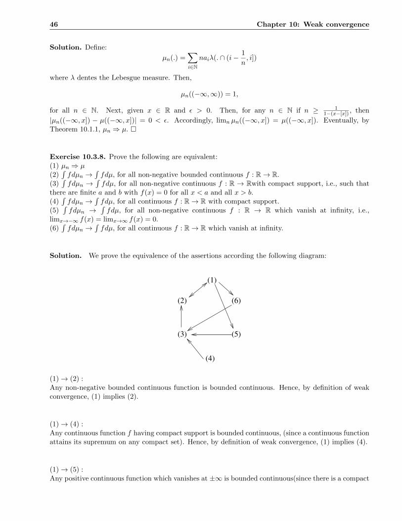
Solution. We prove the equivalence of the assertions according the following diagram:

(1)

(5)

(4)

(3)

(2) (6)

(1)→ (2) :Any non-negative bounded continuous function is bounded continuous. Hence, by definition of weakconvergence, (1) implies (2).

(1)→ (4) :Any continuous function f having compact support is bounded continuous, (since a continuous functionattains its supremum on any compact set). Hence, by definition of weak convergence, (1) implies (4).

(1)→ (5) :Any positive continuous function which vanishes at ±∞ is bounded continuous(since there is a compact

Chapter 10: Weak convergence 47

set [−M,M ] such that |f | ≤ 1 outside of it, implying

|f | ≤ max(1, sup[−M,M ]

|f(x)|) <∞).

Hence, by definition of weak convergence, (1) implies (5).

(1)→ (6) :Any continuous function which vanishes at ±∞ is bounded continuous(since there is a compact set[−M,M ] such that |f | ≤ 1 outside of it, implying

|f | ≤ max(1, sup[−M,M ]

|f(x)|) <∞).

Hence, by definition of weak convergence, (1) implies (5).

(4)→ (3) :Any function satisfying (3) is an special case of (4). Thus, (4) implies (3).



(2)→ (1) :Let f be a bounded continuous function. Then, f+ = max(f, 0) and f− = max(−f, 0) are non-negativebounded continuous functions. Hence, by (2) it follows:

limn

∫fdµn = lim

n

∫f+dµn − lim

n

∫f−dµn =

∫f+dµ−

∫f+dµ =

∫fdµ.

(3)→ (2) :Let f be a non-negative bounded continuous function. Put fM = f1[−M,M ] for M > 0. We claim that:

limn

∫fMdµn =

∫fMdµ for any M > 0.(?)

To prove the assertion, let ε > 0. Then, there are non negative-compact support- continuous functionsgM and hM with hM ≤ fM ≤ gM such that :∫

fMdµ ≤∫gMdµ ≤

∫fMdµ+ ε,∫

fMdµ ≥∫hMdµ ≥

∫fMdµ− ε,


implying: ∫fMdµ− ε ≤

∫hMdµ

= lim infn

∫hMdµn

≤ lim infn

∫fMdµn

≤ lim supn

∫fMdµn

≤ lim supn

∫gMdµn

=

∫gMdµ

≤∫fMdµ+ ε.

Now, since the ε > 0 can be chosen arbitrary, the desired result follows. Next, let (2) does not hold.Therefore, there exist ε0 > 0 and an increasing sequence nk∞k=1 such that |

∫fdµnk −

∫fdµ| > ε0 for

all k ∈ N. On the other hand, using (?) there are large enough M0 > 0 and k0 ∈ N such that :

|∫fdµnk0 −

∫fM0dµnk0 | <

ε04,

|∫fM0dµnk0 −

∫fM0dµ| <

ε04,

|∫fM0dµ−

∫fdµ| <

ε04,

Eventually, an application of triangular inequality shows that:

ε0 < |∫fdµnk0 −

∫fdµ| ≤ |

∫fdµnk0 −

∫fM0dµnk0 |

+ |∫fM0dµnk0 −

∫fM0dµ|

+ |∫fM0dµ−

∫fdµ|

<3ε04,

which is a contradiction.

Exercise 10.3.10. Let f : [0, 1] → (0,∞) be a continuous function such that∫ 10 fdλ = 1 (where λ is

the Lebesgue measure on [0,1]). Define probability measures µ and µn by µ(A) =∫ 10 f1Adλ and

µn(A) =

n∑i=1

f(i/n)1A(i/n)/

n∑i=1

f(i/n).

Chapter 10: Weak convergence 49

(a) Prove that µn ⇒ µ.(b) Explicitly, construct random variables Y and Yn so that L(Y ) = µ, L(Yn) = µn, and Yn → Ywith probability 1.

Solution.(a) Let A be a measurable set with µ(∂A) = 0. Then:

limnµn(A) = lim

n

∑ni=1 f(i/n)1A(i/n)∑n

i=1 f(i/n)

= limn

∑ni=1 f(i/n)1A(i/n)1/n∑n

i=1 f(i/n)1/n

=limn

∑ni=1 f(i/n)1A(i/n)1/n

limn∑n

i=1 f(i/n)1/n

=

∫ 10 f1Adλ∫ 10 fdλ

=

∫ 1

0f1Adλ

= µ(A)

Consequently, by Theorem 10.1.1, µn ⇒ µ.

(b) Let (Ω,F , P ) be Lebesgue measure on [0, 1]. Put

Fn(x) = µn((−∞, x]) = (

∑[nx]i=1 f( in)∑ni=1 f( in)

)1[0,1](x) + 1(1,∞)(x)

and

F (x) = µ((−∞, x]) =

∫ x

0f(t)dt1[0,1](x) + 1(1,∞)(x).

Then, consider :

Yn(w) = infx : Fn(x) ≥ w

= infx ∈ [0, 1] :

[nx]∑i=1

f(i

n) ≥

n∑i=1

f(i

n)w,

and

Y (w) = infx : F (x) ≥ w

= infx ∈ [0, 1] :

∫ x

0f(t)dt ≥ w,

where 0 ≤ w ≤ 1. Now, by the proof of the Theorem 10.1.1, it follows that Yn → Y with probability1.


Chapter 11

Characteristic functions

Exercise 11.5.2. Let µn = δnmod 3 be a point mass at n mod 3.(Thus, µ1 = δ1, µ2 = δ2, µ3 = δ0,µ4 = δ1, µ5 = δ2, µ6 = δ0, etc.)(a) Is µn tight?(b) Does there exist a Borel probability measure µ, such that µn ⇒ µ? (If so, then specify µ.)(c) Does there exist a subsequence µnk , and a Borel probability measure µ , such that µnk ⇒ µ? (Ifso, then specify µnk and µ.)(d) Relate parts (b) and (c) to theorems from this section.

Solution. (a) Yes. Take [a, b] = [0, 3], then, for all ε > 0 and for all n ∈ N :

µn([0, 3]) = δn([0, 3])mod 3 = 1[0,3](n)|n=0,1,2 = 1 > 1− ε.

(b) No. Assume, there exists such a distribution µ. Hence, by Theorem 10.1.1, for any x ∈ R withµ(x) = 0, it follows limn µn((−∞, x]) = µ((−∞, x]). On the other hand, pick x ∈ (0, 1) such thatµ(x) = 0,. Then, µn((−∞, x]) = 1if3|n, 0etc. for all n ∈ N. Therefore, limn µn((−∞, x]) does notexist, a contradiction.

(c) Yes. Put nk = 3k + 1 for k = 0, 1, 2, .... Then, µnk = µ1 = δ1 for k = 0, 1, 2, ..., implying µnk ⇒ δ1.

(d) The sequence µn∞n=1 is a tight sequence of probability measures, satisfying assumptions of theTheorem 11.1.10, and according to that theorem, there exists a subsequence µnk∞k=1 (here, nk = 3k+1for k ∈ N) such that for some probability measure µ (here, µ = δ1), µnk ⇒ µ.

Exercise 11.5.4. Let µ2n = δ0 , and let µ2n+1 = δn, for n = 1, 2, · · · .(a) Does there exist a Borel probability measure µ such that µn ⇒ µ?(b) Suppose for some subsequence µnk∞k=1 and some Borel probability measure ν, we have µnk ⇒ ν.What must ν must be?(c) Relate parts (a) and (b) to Corollary 11.1.11. Why is there no contradiction?

52 Chapter 11: Characteristic functions

Solution. (a) No. Assume, there exists such a distribution µ. Hence, by Theorem 10.1.1, for anyx ∈ R with µ(x) = 0, it follows limn µn((−∞, x]) = µ((−∞, x]). On the other hand, pick x ∈ (0, 1)such that µ(x) = 0 . Then, µn((−∞, x]) = 1if2|n, 0etc. for all n ∈ N. Therefore, limn µn((−∞, x])does not exist, a contradiction.

(b) Since any subsequence µnk∞k=1 including an infinite subsequence of µ2k+1∞k=1 is not weaklyconvergence, we must consider µnk∞k=1 as a subsequence of µ2k∞k=1. In this case, µnk = ν = δ0 forall k ∈ N, implying µnk ⇒ ν.

(c) Since µn∞n=1 is not tight (Take ε = 12 . Then, for any [a, b] ⊆ R and any n ∈ N, if n ≥ bbc+ 1 then

µ2n+1([a, b]) = 0 < 1 − 12 .), the hypothesis of Corollary 11.1.11 is violated. Consequently, there is no

contradiction to the assertion of that Corollary.

Exercise 11.5.6. Suppose µn ⇒ µ. Prove or disprove that µn must be tight.

Solution. First Method:Given ε > 0. Since µ(R) = 1, there is a closed interval [a0, b0] such that:

1− ε

2≤ µ([a0, b0]). (?)

Next, by Theorem 10.1.1(2), there is a positive integer N such that:

|µn([a0, b0])− µ([a0, b0])| ≤ε

2n = N + 1, · · · ,

implying:

µ([a0, b0])−ε

2≤ µn([a0, b0]) n = N + 1, · · · . (??)

Combining (?) and (??) yields:

1− ε ≤ µn([a0, b0]) n = N + 1, · · · . (? ? ?)

Next, for each 1 ≤ n ≤ N, there is a closed interval [an, bn] such that:

1− ε ≤ µn([an, bn]) n = 1, · · · , N. (? ? ??)

Define:

a = min0≤n≤N

(an) b = max0≤n≤N

(bn).

Then, by [an, bn] ⊆ [a, b] for all 0 ≤ n ≤ N , the inequality (? ? ?) and the inequality (? ? ??) we havethat :

1− ε ≤ µn([a, b]) n = 1, 2, · · · .

Second Method:Let φ, φ1, φ2, · · · , be corresponding characteristic functions to the probability measures µ, µ1, µ2, · · · .Then, by Theorem 11.1.14(the continuity theorem) µn ⇒ µ implies, limn φn(t) = φ(t) for all t ∈ R. Onthe other hand, φ is continuous on the R. Thus, according to Lemma 11.1.13, µn is tight.

Chapter 11: Characteristic functions 53

Exercise 11.5.8. Use characteristic functions to provide an alternative solution of Exercise 10.3.2.

Solution. Since X and Yn are independent, it follows:

φZn(t) = φX(t)φYn(t) = φX(t)(exp(it).1

n+ (1− 1

n))for all(n ∈ N).

Therefore, limn φZn(t) = φX(t) for all t ∈ R. Hence, by Theorem 11.1.14 (the continuity theorem),L(Zn)⇒ L(X).

Exercise 11.5.10. Use characteristic functions to provide an alternative solution of Exercise 10.3.4.

Solution. Let µn ⇒ µ and µn ⇒ ν . Then, by Theorem 11.1.14, limn φn(t) = φµ(t) and limn φn(t) =φν(t) for all t ∈ R. Hence, φµ(t) = φν(t) for all t ∈ R. Eventually, by Corollary 11.1.7., µ = ν.

Exercise 11.5.12. Suppose that for n ∈ N, we have P (Xn = 5) = 1n and P (Xn = 6) = 1− 1

n .(a) Compute the characteristic function φXn(t), for all n ∈ N and all t ∈ R.(b) Compute limn→∞ φXn(t).(c) Specify a distribution µ such that limn→∞ φXn(t) =

∫exp(itx)µ(dx) for all t ∈ R.

(d) Determine (with explanation) whether or not L(Xn)⇒ µ.

Solution. (a)

φXn(t) = E(exp(itXn)) = exp(5it)n + (n−1) exp(6it)

n t ∈ R.(b)limn→∞ φXn(t) = exp(6it) t ∈ R.(c)µ = δ6.(d)As a result of the Theorem 11.1.14 (the continuity theorem), L(Xn)⇒ δ6.

Exercise 11.5.14. Let X1, X2, · · · be i.i.d. with mean 4 and variance 9. Find values C(n, x), forn ∈ N and x ∈ R , such that as n→∞, P (X1 +X2 + · · ·+Xn ≤ C(n, x)) ≈ Φ(x).

Solution. As in Corollary 11.2.3:

P (Sn − nm√

nv≤ x) = Φ(x) asn→∞

Thus :

Φ(x) = P (Sn − 4n√

9n≤ C(n, x)− 4n√

9n) = Φ(

C(n, x)− 4n√9n

),

asn→∞, and injectivity of Φ implies :

x =C(n, x)− 4n√

9n,

54 Chapter 11: Characteristic functions

or :C(n, x) =

√9nx+ 4n.

Exercise 11.5.16. Let X be a random variable whose distribution L(X) is infinitely divisible. Leta > 0 and b ∈ R, and set Y = aX + b, prove that L(Y ) is infinitely divisible.

Solution. Given n ∈ N. Since the distribution L(X) is infinitely divisible, there is a distributionνn such that if Xk ∼ νn , 1 ≤ k ≤ n, are independent random variables, then

∑nk=1Xk ∼ L(X) or,

equivalently, there is a distribution νn such that if Xk , 1 ≤ k ≤ n, with FXk(x) = νn((−∞, x]), (x ∈ R)are independent, then F∑n

k=1Xk(x) = FX(x), (x ∈ R). The latest assertion yields that there is a

distribution ωn defined by ωn((−∞, x]) = νn((−∞, x−ba ]), (x ∈ R)such that if Xk , 1 ≤ k ≤ n, withFaXk+b(x) = ωn((−∞, x]), (x ∈ R) are independent, then F∑n

k=1(aXk+b)(x) = FaX+b(x), (x ∈ R).

Accordingly, the distribution L(Y ) is infinitely divisible, as well.

Exercise 11.5.18. Let X,X1, X2, · · · be random variables which are uniformly bounded , i.e. thereis M ∈ R with |X| ≤ M and |Xn| ≤ M for all n. Prove that L(Xn) ⇒ L(X) if and only if E(Xk

n) →E(Xk) for all k ∈ N.

Solution. Let L(Xn) ⇒ L(X). Then, by Theorem 10.1.1, limn

∫fd(L(Xn)) =

∫fd(L(X)) for any

bounded Borel measurable function f with L(X)(Df ) = 0. Put fk(x) = xk(k ∈ N). Then, since|fk| ≤Mk <∞(k ∈ N), it follows that:

limnE(Xk

n) = limn

∫xkd(L(Xn)) =

∫xkd(L(X)) = E(Xk),

for all k ∈ N.

Conversely, let E(Xkn)→ E(Xk) for all k ∈ N. Since |X| ≤M ,

|MX(s)| = |E(esX)| ≤ max(e−M , eM ) <∞

for all |s| < 1. Therefore, by Theorem 11.4.3, L(X) is determined by its moments. Now, the desiredassertion follows from Theorem 11.4.1.

Chapter 12

Decompositions of probability laws

Exercise 12.3.2. Let X and Y be discrete random variables (not necessarily independent), and letZ = X + Y . Prove that L(Z) is discrete.

Solution. Let F be an an uncountable set of positive numbers. Then,∑

x∈F x = +∞. Thus, thesummation in the definition of Borel probability measure of discrete random variable is, in fact, takenover a countable set for which the probability of each of its elements is nonzero. Hence, in the equalities∑

x∈RL(X)(x) = L(X)(R)

and ∑y∈RL(Y )(y) = L(Y )(R),

the sets AX = x ∈ R : L(X)(x) > 0 and BY = y ∈ R : L(Y )(y) > 0 are countable. On theother hand, for any z ∈ R we have L(X + Y )(z) ≥ P (X = x, Y = z − x) > 0for somex ∈ R, and thecorresponding ordered pair (x, z − x) in the recent result is an element of the countable set AX ×BY .Hence, the set CZ = z ∈ R : L(X + Y )(z) > 0 is countable. Thus:∑

z∈RL(X + Y )(z) =

∑z∈CZ

L(X + Y )(z)

= L(X + Y )(CZ) + 0

= L(X + Y )(CZ) + L(X + Y )(CcZ)

= L(X + Y )(R).

Exercise 12.3.4. Let X and Y be random variables, with L(Y ) absolutely continuous, and letZ = X + Y.(a) Assume X and Y are independent. Prove that L(Z) is absolutely continuous, regardless of thenature of L(X).(b) Show that if X and Y are not independent, then L(Z) may fail to be absolutely continuous.

56 Chapter 12: Decompositions of probability laws

Solution. (a) Let for a Borel measurable set A ⊆ R, λ(A) = 0. Hence, λ(A − x) = 0, for all x ∈ R.Then, by Corollary 12.1.2.(Radon-Nikodym Theorem), L(Y )(A−x) = 0 for all x ∈ R. Now, by Theorem9.4.5.:

L(Z)(A) =

∫L(Y )(A− x)L(X)dx = 0.

Eventually, by another application of the Corollary 12.1.2.(Radon-Nikodym Theorem), the desiredresult follows.

(b) First example:Put X = Z and Y = −Z, where Z ∼ N(0, 1). Then, X + Y = 0, which is clearly discrete.

Second example:Similar to Exercise 6.3.5., let X ∼ N(0, 1), Y = XU where X and U are independent and P (U = 1) =P (U = −1) = 1

2 . Then, X and Y are dependent. Put Z = X + Y. Then, for the Borel measurable setA = 0, λ(A) = 0. But, L(Z)(A) = 1

2 6= 0 (Check!).

Exercise 12.3.6. Let A,B,Z1, Z2, · · · be i.i.d., each equal to +1 with probability 2/3, or equal to 0with probability 1/3. Let Y =

∑∞i=1 Zi2

−i as at the beginning of this section (so ν = L(Y ) is singularcontinuous), and let W ∼ N(0, 1). Finally, let X = A(BY + (1 − B)W ), and set µ = L(X). Find adiscrete measure µdisc, an absolutely continuous measure µac, and a singular continuous measure µs,such that µ = µdisc + µac + µs.

Solution. Using conditional probability, for any Borel measurable set U ⊆ R , it follows:

L(X)(U) = P (X ∈ U)

= P (X ∈ U |A = 0)P (A = 0)

+ P (X ∈ U |A = 1)P (A = 1)

=1

3P (0 ∈ U)

+2

3P (BY + (1−B)W ∈ U)

=1

3δ0(U)

+2

3(P (BY + (1−B)W ∈ U |B = 0)P (B = 0)

+ P (BY + (1−B)W ∈ U |B = 1)P (B = 1))

=1

3δ0(U) +

2

3(1

3P (W ∈ U) +

2

3P (Y ∈ U))

=1

3δ0(U) +

2

9L(W )(U) +

4

9L(Y )(U).

Accordingly, L(X) = 13δ0 + 2

9L(W ) + 49L(Y ).

Exercise 12.3.8. Let µ and ν be probability measures with µ ν and ν µ. (This is sometimes

Chapter 12: Decompositions of probability laws 57

written as µ ≡ ν.) Prove that dµdν > 0 with µ-probability 1, and in fact dν

dµ = 1dµdν

.

Solution. By Exercise 12.3.7., dµdρ = dµ

dνdνdρ with ρ-probability 1. We claim that :

dµ

dν=

dµdρ

dνdρ

ν − probability1.(?)

To prove the above equality we notice that :

ν(w :dν

dρ= 0) =

∫w: dν

dρ=0

dν

dρdρ = 0,

consequently, dνdρ > 0, ν − probability-1 . Hence, (?) holds ν − probability-1. Of course on the set

w : dνdρ = 0, the right hand side of (?) can be defined as zero. Now, let ρ = µ. Then, dν

dµ >

0, ν − probability-1 and dµdν = 1

dνdµ

. Eventually, the final assertion follows by symmetric relationship of µ

and ν.

Exercise 12.3.10. Let µ and ν be absolutely continuous probability measures on R (with the Borelσ algebra), with φ = µ− ν. Write down an explicit Hahn decomposition R = A+ ∪A− for φ.

Solution. First, since µ and ν are absolutely continuous , they are countable additive (In fact,

µ(∪∞n=1An) =

∫1∪∞n=1An

dµ

dλdλ

=

∫ ∞∑n=1

1Andµ

dλdλ

=∑∫ ∞

n=11An

dµ

dλdλ

=

∞∑n=1

µ(An),

where the union is considered as the disjoint one. ) Next, by linearity it follows that φ = µ − νis countable additive, as well. Finally, by Remark (3), Page 145, µ(E) = φ(E ∩ A+) and ν(E) =−φ(E ∩A−).

58 Chapter 12: Decompositions of probability laws

Chapter 13

Conditional probability and expectation

Exercise 13.4.2. Let G be a sub-σ-algebra, and let A be any event. Define the random variable X tobe the indicator function 1A. Prove that E(X|G) = P (A|G) with probability 1.

Solution. By definition, both of E(1A|G) and P (A|G) are G measurable random variables. Next, byequations (13.2.1) and (13.2.2):

E(P (A|G)1G) = P (A ∩G)

= E(1A∩G)

= E(1A1G)

= E(E(1A|G)1G),

for any G ∈ G. Consequently, E(1A|G) = P (A|G) with probability 1.

Exercise 13.4.4. Let X and Y be random variables with joint distribution given by L(X,Y ) = dP =f(x, y)λ2(dx, dy), where λ2 is two dimensional Lebesgue measure, and f : R2 → R is a non-negativeBorel measurable function with

∫R2 fdλ2 = 1. Show that we can take P (Y ∈ B|X) =

∫B gX(y)λ(dy)

and E(Y |X) =∫R ygX(y)λ(dy), where the function gx : R → R is defined by gx(y) = f(x,y)∫

R f(x,t)λ(dt)

whenever∫R f(x, t)λ(dt) is positive and finite, otherwise (say) gx(y) = 0.

Solution. First, let YB(x) =∫B gX(y)λ(dy). Then, YB(x) is a σ(X)-measurable random variable and

for A = (Y ∈ B) in Definition 13.1.4 an application of the Fubini’s Theorem in Real Analysis yields:

E(YB(x)1X∈S) = E(

∫BgX(y)λ(dy)1X∈S)

=

∫S

∫BgX(y)fX(x)λ(dy)λ(dx)

=

∫ ∫(S×B)

f(x, y)λ2(dx, dy)

= P ((Y ∈ B) ∩ X ∈ S),

60 Chapter 13: Conditional probability and expectation

for all Borel S ⊆ R, proving that P (Y ∈ B|X) =∫B gX(y)λ(dy) with probability 1.

Second, by considering E(1B|X) = P (Y ∈ B|X), the second equation follows from the first equationfor the special case Y = 1B. Now, by usual linearity and monotone convergence arguments the secondequality follows for general Y .

Exercise 13.4.6. Let G be a sub-σ-algebra, and let X and Y be two independent random variables.Prove by example that E(X|G) and E(Y |G) need not be independent.

Solution. Consider the sub-σ-algebra G = φ,Ω . Let X,Y ∼ N(0, 1) be independent. Then:

E(X|G) : Ω→ RE(X|G)(w) = E(X) = 0,

and,

E(Y |G) : Ω→ RE(Y |G)(w) = E(Y ) = 0.

Consequently, E(X|G) = E(Y |G), showing that they are not independent.

Exercise 13.4.8. Suppose Y is G-measurable. Prove that V ar(Y |G) = 0.

Solution. Since Y and E(Y |G) are G-measurable, it follows that Y − E(Y |G) is G-measurable, too.Now, an application of Proposition 13.2.6 yields:

V ar(Y |G) = E((Y − E(Y |G))2|G)

= (Y − E(Y |G))E(Y − E(Y |G)|G)

= (Y − E(Y |G))(E(Y |G)− E(Y |G))

= 0.

Exercise 13.4.10. Give an example of jointly defined random variables which are not independent,but such that E(Y |X) = E(Y ) w.p. 1.

Solution. Let X = Y = 1. Then, E(Y ) = 1 is a σ(X)-measurable random variable and:

E(E(Y )1X∈S) = E(1.1X∈S) = E(Y 1X∈S)

for any Borel S ⊆ R. Accordingly, by Definition 13.1.4 the desired result follows.

Chapter 13: Conditional probability and expectation 61

Exercise 13.4.12. Let Zn be independent, each with finite mean. Let X0 = a, and Xn = a+ Z1 +...+ Zn for n ≥ 1. Prove that

E(Xn+1|X0, X1, ..., Xn) = Xn + E(Zn+1).

Solution. Let G = σ(X0, X1, ..., Xn). Then, Xn and E(Zn+1) are G measurable and so is Xn+E(Zn+1).Since Z1, Z2, ..., Zn, Zn+1 are independent , by Exercise 3.6.6 and induction it follows that Zn+1 and1G are independent for all G ∈ G. Consequently:

E((Xn + E(Zn+1))1G) = E(Xn1G) + E(E(Zn+1)1G)

= E(Xn1G) + E(Zn+11G)

= E((Xn + Zn+1)1G)

= E(Xn+11G),

for all G ∈ G. Thus, E(Xn+1|X0, X1, ..., Xn) = Xn + E(Zn+1) w.p.1.

62 Chapter 13: Conditional probability and expectation

Chapter 14

Martingales

Exercise 14.4.2. Let Xn be a submartingale, and let a ∈ R. Let Yn = max(Xn, a). Prove thatYn is also a submartingale.

Solution. First,

E(|Yn|) ≤ E(max(|Xn|, |a|)) ≤ E(|Xn|) + |a| <∞,

for all n ∈ N. Second, using conditional version of Exercise 4.5.2, it follows that:

E(Yn+1|σ(Y0, ..., Yn)) = E(max(Xn+1, a)|σ(X0, ..., Xn))

≥ max(E(Xn+1|σ(X0, ..., Xn)), a)

≥ max(Xn, a)

= Yn,

W.P 1, for all n ∈ N.

Exercise 14.4.4. The conditional Jensen’s inequality states that if φ is a convex function, thenE(φ(X)|G) ≥ φ(E(X|G)).(a) Assuming this, prove that if Xn is a submartingale, then so is φ(Xn) whenever φ is non-decreasing and convex with E(|φ(Xn)|) <∞, for all n.(b) Show that the conclusion of the two previous exercises follow from part (a).

Solution. (a) First, by assumption E(|φ(Xn)|) < ∞, for all n. Second, using conditional Jensen’sinequality if follows that :

E(φ(Xn+1)|σ(φ(X0), ..., φ(Xn))) = E(φ(Xn+1)|σ(X0, ..., Xn))

≥ φ(E(Xn+1|σ(X0, ..., Xn)))

≥ φ(Xn),

w.p. 1, for all n ∈ N.

64 Chapter 14: Martingales

(b) It is sufficient to consider non-decreasing and convex functions φ1(x) = max(x, a) and φ2(x) = x2

in Exercise 14.4.2, and Exercise 14.4.3, respectively.

Exercise 14.4.6. Let Xn be a stochastic process, let τ and ρ be two non-negative-integer valuedrandom variables , and let m ∈ N.(a) Prove that τ is a stopping time for Xn if and only if τ ≤ n ∈ σ(X0, ..., Xn) for all n ≥ 0.(b) Prove that if τ is a stopping time, then so is min(τ,m).(c) Prove that if τ and ρ are stopping times for Xn, then so is min(τ, ρ).

Solution. (a) Let τ satisfies τ ≤ n ∈ σ(X0, ..., Xn) for all n ≥ 0. Then,

τ = n = τ ≤ n⋂τ ≤ n− 1c ∈ σ(X0, ..., Xn),

for all n ≥ 0. Thus, τ is a stopping time.Conversely, let τ be a stopping time and let n ≥ 0 be given. Then,

τ = m ∈ σ(X0, ..., Xn)

for all 0 ≤ m ≤ n, and , consequently,

τ ≤ n =

n⋃m=0

τ = m ∈ σ(X0, ..., Xn).

(b) First, min(τ,m) is a non-negative integer-valued random variable. Second, let n ≥ 0 be given.Then,

min(τ,m) ≤ n = τ ≤ n⋃m ≤ n,

and depending on whether m ≤ n or m > n we have that m ≤ n = Ω or m ≤ n = φ, respectively.Therefore, min(τ,m) ≤ n ∈ σ(X0, ..., Xn). Now, the assertion follows by part (a).

(c) First, since τ and ρ are non-negative-integer valued random variables, min(τ, ρ) has the sameproperties. Second, let n ≥ 0 be given. Then, by part (a), τ ≤ n, ρ ≤ n ∈ σ(X0, ..., Xn) and,consequently,

min(τ, ρ) ≤ n = τ ≤ n⋃ρ ≤ n ∈ σ(X0, ..., Xn).

Finally, another application of part (a) proves the desired result.

Exercise 14.4.8. Let Xn be simple symmetric random walk, with X0 = 0. Let τ = infn ≥ 5 :Xn+1 = Xn + 1 be the first time after 4 which is just before the chain increases. Let ρ = τ + 1.(a) Is τ a stopping time? Is ρ a stopping time?(b) Use Theorem 14.1.5., to compute E(Xρ).(c) Use the result of part (b) to compute E(Xτ ). Why does this not contradict Theorem 14.1.5.?

Solution. (a) No. τ is not a stopping time because

τ = n = X6 6= X5 + 1, ..., Xn 6= Xn−1 + 1, Xn+1 = Xn + 1/∈ σ(X0, ..., Xn)

Chapter 14: Martingales 65

for all n ≥ 6.Yes. First, ρ = τ + 1 is a non- negative integer-valued random variable. Second, ρ = n = τ =n− 1 = φ if 0 ≤ n ≤ 5, X6 6= X5 + 1, ..., Xn−1 6= Xn−2 + 1, Xn = Xn−1 + 1 if n ≥ 6, implying thatτ = n ∈ σ(X0, ..., Xn).

(b) E(Xρ) = E(X0) = 0.

(c) By definition of τ, we have Xρ = Xτ + 1 and consequently, E(Xτ ) = E(Xρ)− 1 = −1. This resultdoes not contradict Theorem 14.1.5. due to the fact that τ is not a stopping time and, consequently,the assumption of that Theorem is violated.

Exercise 14.4.10. Let 0 < a < c be integers. Let Xn be simple symmetric random walk, startedat X0 = a. Let τ = infn ≥ 1 : Xn = 0, orc.(a) Prove that Xn is a martingale.(b) Prove that E(Xτ ) = a.(c) Use this fact to derive an alternative proof of the gambler’s ruin formula given in Section 7.2, forthe case p = 1/2.

Solution. (a) First, let Yn = Xn − a(n ∈ N). Then, by equation 14.0.2, it is a martingale. Hence,

E(|Xn|) ≤ E(|Yn|) + |a| <∞,

for all n ≥ 0. Second, considering the definition of simple random walk in page 75, it follows that:

E(Xn+1|σ(X0, ..., Xn)) = E(Xn + Zn+1|σ(X0, ..., Xn))

= Xn + E(Zn+1|σ(X0, ..., Xn))

= Xn + E(Zn+1|σ(Z0, ..., Zn))

= Xn + E(Zn+1)

= Xn.

for all n ≥ 0.

(b) By τ = min(τ0, τc) and P (τ0 <∞) = 1 = P (τc <∞), it follows that;

P (τ <∞) = P (τ0 <∞∪ τc <∞) = 1.

Next, |Xn|1n≤τ ≤ c1n≤τ for all n ≥ 0. Consequently, by Corollary 14.1.7, it follows that E(Xτ ) =E(X0) = a.

(c) By part (b),

a = E(Xτ ) = 0.P (Xτ = 0) + c.P (Xτ = c) = cP (τc < τ0) = cS(a),


implying S(a) = ac .

Exercise 14.4.12. Let Sn and τ be as in Example 14.1.13.(a) Prove that E(τ) <∞.(b) Prove that Sτ = −τ + 10.

Solution. First, we claim that

P (τ > 3m) ≤ (7

8)m,

for all m ∈ N. To prove it we use induction. Let m = 1, then

P (τ > 3) = 1− P (τ = 3) = 1− 1

8=

7

8.

Assume the assertion holds for positive integer m > 1. Then,

P (τ > 3(m+ 1)) = P (τ > 3m ∩ (r3m+1, r3m+2, r3m+3) 6= (1, 0, 1))

= P (τ > 3m)P ((r3m+1, r3m+2, r3m+3) 6= (1, 0, 1))

≤ (7

8)m.(

7

8)

= (7

8)m+1,

proving the assertion for positive integer m+ 1. Second, using Proposition 4.2.9, we have that

E(τ) =∞∑k=0

P (τ > k)

=∞∑m=1

(P (τ > 3m− 1) + P (τ > 3m− 2) + P (τ > 3m− 3))

≤ 3∞∑m=1

P (τ > 3m− 3)

= 3 + 3

∞∑m=1

P (τ > 3m)

≤ 3 + 3

∞∑m=1

(7

8)m

< ∞.

(b) We consider τ − 2 different players . Each of those numbered 1 to τ − 3 has bet and lost $1 (Theperson has lost the $1 bet or, has won the $1 bet and then has lost the $2 bet or, has won the $1bet and the next $2 bet but has lost the $4 bet. In each of these three different cases, the person hastotally lost $1. ). The person numbered τ − 2 has won all of $1, $2, and $4 bets successively and hastotally won $7. Accordingly,

Sτ = (τ − 3)(−1) + 1.7 = −τ + 10.


Exercise 14.4.14. Why does the proof of Theorem 14.1.1 fail if M =∞?

Solution. Let Xn∞n=0 be defined by X0 = 0 and Xn =∑n

i=1 Zi where Zi are i.i.d, with P (Zi =+1) = P (Zi = −1) = 1

2 for all i ∈ N. Then, by Exercise 13.4.2, it is a martingale. Now, by Exercise4.5.14(c),

E(∞∑i=1

Zi) 6=∞∑i=1

E(Zi),

showing that the Proof of Theorem 14.1.1 fails for the case M =∞.

Exercise 14.4.16. Let Xn be simple symmetric random walk, with X0 = 10. Let τ = minn ≥1 : Xn = 0, and let Yn = Xmin(n,τ). Determine (with explanation) whether each of the followingstatements is true or false.(a) E(X200) = 10.(b) E(Y200) = 10.(c) E(Xτ ) = 10.(d) E(Yτ ) = 10.(e) There is a random variable X such that Xn → X a.s.(f) There is a random variable Y such that Yn → Y a.s.

Solution. (a) True. Since Xn is a martingale, using equation 14.0.4. it follows that E(X200) =E(X0) = 10.

(b) True. Consider the stopping time ρ = min(τ, 200). Then, 0 ≤ ρ ≤ 200 and, therefore, by Corollary14.1.3,

E(Y200) = E(Xρ) = E(X0) = 10.

(c) False. Since P (Xτ = 0) = 1, it follows that E(Xτ ) = 0 6= 10.

(d) False. Since Yτ(w)(w) = Xmin(τ(w),τ(w))(w) = Xτ(w)(w) for all w ∈ Ω, it follows that E(Yτ ) =E(Xτ ) = 0 6= 10.

(e) False. Since lim supnXn = +∞ and lim infnXn = −∞, there is no finite random variable X withlimnXn = X a.s.

(f) True. For the non-negative martingale Yn an application of Corollary 14.2.2, yields existence ofa finite random variable Y with limn Yn = Y a.s.

Exercise 14.4.18. Let 0 < p < 1 with p 6= 1/2, and let 0 < a < c be integers. Let Xn be simplerandom walk with parameter p , started at X0 = a. Let τ = infn ≥ 1 : Xn = 0, orc.(a) Compute E(Xτ ) by direct computation.


(b) Use Wald’s theorem part (a) to compute E(τ) in terms of E(Xτ ).(c) Prove that the game’s expected duration satisfies

E(τ) = (a− c[((1− p)/p)a − 1]/[((1− p)/p)c − 1])/(1− 2p).

(d) Show that the limit of E(τ) as p→ 1/2 is equal to a(c− a).

Solution. (a)

E(Xτ ) = c.P (Xτ = c) + 0.P (Xτ = 0) = c.(1− (1−pp )a

1− (1−pp )c).

(b) From E(Xτ ) = a+ (p− q)E(τ) it follows that

E(τ) =1

q − p(a− E(Xτ )).

(c) By parts (a) and (b), it follows that

E(Xτ ) =1

1− 2p(a− c.(

1− (1−pp )a

1− (1−pp )c)).

(d) Applying I.Hopital’s rule, it follows that :

limp→1/2

E(τ) = limp→1/2

a(1− ( 1−pp

)c)− c(1− ( 1−pp

)a)

(1− 2p)(1− ( 1−pp

)c)

=Hop limp→1/2

−a.c( 1−pp

)c−1(−1p2

)− c(−a)( 1−pp

)a−1(−1p2

)

−2(1− ( 1−pp

)c) + (1− 2p)(−c( 1−pp

)c−1(−1p2

))

= limp→1/2

ac.( 1−pp

)a−1 − ( 1−pp

)c−1

2p2(1− ( 1−pp

)c)− (1− 2p)c( 1−pp

)c−1

=Hop limp→1/2

ac.(a− 1)( 1−p

p)a−2(−1

p2)− (c− 1)( 1−p

p)c−2(−1

p2)

4p(1− ( 1−pp

)c) + 2p2(−c( 1−pp

)c−1(−1p2

)) + 2c( 1−pp

)c−1 − (1− 2p)c(c− 1)( 1−pp

)c−2(−1p2

)

= ac.(a− 1)(−4)− (c− 1)(−4)

0 + 2c+ 2c− 0

= a(c− a).

Exercise 14.4.20. Let Xn be a martingale with |Xn+1 − Xn| ≤ 10 for all n. Let τ = infn ≥ 1 :|Xn| ≥ 100.(a) Prove or disprove that this implies that P (τ <∞) = 1.(b) Prove or disprove that this implies there is a random variable X with Xn → X a.s.(c) Prove or disprove that this implies that

P (τ <∞, or there is a random variable X withXn → X) = 1.

Solution. (a) No. As a counterexample, let X0 = 0 and Xn =∑n

i=1 Zi where Zi are i.i.d withP (Zi = 2−i) = 1

2 and P (Zi = −2−i) = 12 for all i ∈ N. Since, E(Zi) = 0 for all i ∈ N, by Exercise

13.4.12, Xn is a martingale. Clearly, |Xn+1 −Xn| < 2 < 10 for all n ∈ N. But,

|Xn| = |n∑i=1

Zi| ≤n∑i=1

|Zi| < 2


for all n ∈ N, implying τ = inf φ =∞, and consequently, P (τ <∞) = 0 6= 1.

(b) No. As a counterexample, consider the simple symmetric random walk with X0 = 0. In this case,|Xn+1 − Xn| < 2 ≤ 10 for all n, however, lim supnXn = +∞ and lim infnXn = −∞, showing thatthere is no finite random variable X with limnXn = X a.s.(c) Yes. Define :

A∗ = lim supn

Xn = − lim infn

Xn = +∞,

andB = there is a random variable X withXn → X.

We claim that P (A∗ ∪ B) = 1. To do this, let a ∈ N and define ρ = infn ≥ 1 : Xn ≥ a. Then,Xmin(ρ,n) is a martingale satisfying :

supnE(X+

min(ρ,n)) ≤ a+ E(supn|Xn+1 −Xn|) ≤ a+ 10 <∞.

Thus, by Theorem 14.2.1, Xmin(ρ,n) converges a.s. Hence, Xn converges a.s. on ρ = ∞ =supnXn < a. Let a→∞, then it follows that Xn converges a.s. on supnXn <∞. A symmetricargument applied to −Xn shows that Xn converges a.s. on infnXn > −∞, proving our claim.Now, since τ <∞ ⊇ A∗, the desired result is proved.


Chapter 15

General stochastic processes

Exercise 15.1.6. Let X1, X2, ... be independent, with Xn ∼ µn.(a) Specify the finite dimensional distributions µt1,t2,...,tk for distinct non-negative integers t1 < t2 <... < tk.(b) Prove that these µt1,t2,...,tk satisfy (15.1.1) and (15.1.2).(c) Prove that Theorem 7.1.1 follows from Theorem 15.1.3.

Solution. (a) Since the σ-algebra of k-dimensional Borel sets is generated by the class of all boundedrectangles HR =

∏kn=1 In where In = (an, bn], (1 ≤ n ≤ k) it is sufficient to specify the distribution

µt1,t2,...,tk on HRs. Now, we have that:

µt1,t2,...,tk(

k∏n=1

In) = P (Xtn ∈ In : 1 ≤ n ≤ k)

=k∏

n=1

P (Xtn ∈ In)

=k∏

n=1

µtn(In).(?)

(b) To prove (15.1.1), several consecutive applications of Proposition 3.3.1 on the both sides of theequality (?) in part (a) imply that:

µt1,t2,...,tk(k∏

n=1

Hn) =k∏

n=1

µtn(Hn)

=

k∏n=1

µts(n)(Hs(n))

= µts(1),ts(2),...,ts(k)(

k∏n=1

Hs(n)),

72 Chapter 15: General stochastic processes

for all Borel H1, H2, ...,Hk ⊆ R and all permutations (s(n))kn=1 of (n)kn=1.To prove (15.1.2) , by a similar argument used for the proof of (15.1.1), it follows that :

µt1,t2,...,tk(H1 ×H2 × ...×Hk−1 × R) =

k−1∏n=1

µtn(Hn)µtk(R)

=k−1∏n=1

µtn(Hn)

= µt1,t2,...,tk−1(H1 ×H2 × ...×Hk−1),

for all Borel H1, H2, ...,Hk−1 ⊆ R.

(c) We consider the family of Borel probability measures µt1,t2,...,tk : k ∈ N, ti ∈ Ndistinct withµt1,t2,...,tk defined by

µt1,t2,...,tk(

k∏n=1

Hn) =

k∏n=1

µtn(Hn),

for all Borel H1, H2, ...,Hk ⊆ R. Then, by part (b) it satisfies the consistency conditions (C1) and (C2).Consequently, by Theorem 15.1.3, there is a probability space (RN,FN, P ) and random variables Xndefined on that triple such that

µt1,t2,...,tk(H) = P ((Xt1 , Xt2 , ..., Xtk) ∈ H), (??)

for all k ∈ N, distinct t1, ..., tk ∈ N and Borel H ⊆ Rk. Now, put

H = R× ...× R×Hn × R...× R,

where Hn ⊆ R is Borel (1 ≤ n ≤ k). Then, by (??) :

µtn(Hn) = P (Xtn ∈ Hn) = Ltn(Hn),

for all n ∈ N.

Exercise 15.2.4. Consider a Markov chain which is φ irreducible with respect to some non-zero σ-finite measure ψ, and which is periodic with corresponding disjoint subsets X1, ...,Xd. Let B = ∪iXi.(a) Prove that Pn(x,Bc) = 0 for all x ∈ B.(b) Prove that ψ(Bc) = 0.(c) Prove that ψ(Xi) > 0 for some i.

Solution. (a) We prove the assertion by induction. Let n = 1 and x ∈ B = ∪di=1Xi. Then, there existsan unique 1 ≤ i ≤ d such that x ∈ Xi, and consequently, P (x,Xi+1) = 1 if 1 ≤ i ≤ d−1 or P (x,X1) = 1if i = d. Hence,

0 ≤ P (x,Bc) ≤ P (x,X ci+1) = 0 if 1 ≤ i ≤ d− 1

or

0 ≤ P (x,Bc) ≤ P (x,X c1 ) = 0 if i = d,

Chapter 15: General stochastic processes 73

implying P 1(x,Bc) = 0. Next, assume the assertion holds for positive integer n > 1. Then, byPn(z,Bc) = 0(z ∈ Bc) it follows that:

Pn+1(x,Bc) =

∫XP (x, dz)Pn(z,Bc)

=

∫BP (x, dz)Pn(z,Bc) +

∫BcP (x, dz)Pn(z,Bc)

= 0,

proving the assertion for positive integer n+ 1.

(b) Since τBc = infn ≥ 0 : Xn ∈ Bc = inf φ = ∞, it follows that Px(τBc < ∞) = 0, for all x /∈ Bc,and, consequently, ψ(Bc) = 0.

(c) Using part (b), we have that:

d∑i=1

ψ(Xi) = ψ(B) = ψ(X )− ψ(Bc) = ψ(X ) > 0,

implying that ψ(Xi) > 0 for some 1 ≤ i ≤ d.

Exercise 15.2.6. (a) Prove that a Markov chain on a countable state space X is φ-irreducible if andonly if there is j ∈ X such that Pi(τj <∞) > 0, for all i ∈ X .(b) Give an example of a Markov chain on a countable state space which is φ- irreducible, but whichis not irreducible in the sense of Subsection 8.2.

Solution. (a) Let the given Markov chain on the countable state space X be φ irreducible. Then, forsome A = j ∈ F with ψ(A) > 0, we have τA = τj implying Pi(τj <∞) > 0 for all i ∈ X . Conversely,let there is j ∈ X such that Pi(τj <∞) > 0 for all i ∈ X . Then, we consider the σ-finite measure ψ onF defined by:

ψ(A) = δj(A),

for all A ∈ F . Now, let A ∈ F with ψ(A) > 0, then j ∈ A implying that τA ≤ τj and consequently,Pi(τA <∞) ≥ Pi(τj <∞) > 0 for all i ∈ X .

(b) Consider the Markov chain given in the solution of Exercise 8.5.20(a), which is reducible in thesense of Subsection 8.2. However, for j = 2 we have that:

Pi(τ2 <∞) = P (∃n ≥ 0 : Xn = 2|X0 = i)

≥∑

i1,...,in−1

pii1pi1i2 ...pin−2in−1pin−22

> 0,


for i = 1, 2. Hence, by part (a), this Markov chain is φ-irreducible.

Exercise 15.2.8. Consider a discrete Markov chain with state space X = R, and with transitionprobabilities such that P (x, ·) is uniform on the interval [x− 1, x+ 1]. Determine whether or not thischain is φ-irreducible.

Solution. Yes, this chain is φ-irreducible. Indeed, P (x, ·) has positive density (with respect to Lebesguemeasure) throughout [x − 1, x + 1]. Then, by the convolution formula, P 2(x, ·) has positive densitythroughout [x− 2, x+ 2]. By induction, Pn(x, ·) has positive density throughout [x−n, x+n]. Now, ifA ⊆ X has positive Lebesgue measure, then A∩ [x−n, x+n] must have positive Lebesgue measure forsome n ∈ N. It then follows that Pn(x,A) > 0. Hence, the chain is φ-irreducible where φ is Lebesguemeasure.

Exercise 15.2.10. Consider the Markov chain with X = R, and with P (x, .) = N(x, 1) for each x ∈ X .(a) Prove that this chain is φ-irreducible and aperiodic.(b) Prove that his chain does not have a stationary distribution. Relate this to Theorem 15.2.3.

Solution. (a) Here P (x, ·) has an everywhere-positive density (with respect to Lebesgue measure). Itfollows that if A ⊆ X has positive Lebesgue measure, then P (x,A) > 0 for all x ∈ X. So, the chain isφ-irreducible where φ is Lebesgue measure. As for aperiodicity, if X1, . . . ,Xd is a periodic decomposi-tion for some d ≥ 2, then if x1 ∈ X1 then P (x1,X2) > 0. This implies that X2 has positive Lebesguemeasure, which in turn implies that P (x,X2) > 0 for all x ∈ X , even for x ∈ X2. This contradictsthe assumption of periodic decomposition. So, no such periodic decomposition exists, i.e. the chain isaperiodic.(b) This chain is equivalent to adding an independent N(0, 1) random variable at each iteration. So, ifa stationary probability distribution π(·) existed, it would have to satisfy the property that if X ∼ π(·)and Y ∼ N(0, 1) are independent, then X + Y ∼ π(·). It would follow by induction that if Y1, Y2, . . .are i.i.d. ∼ N(0, 1) (and independent of X), then Zn ≡ X + Y1 + . . . + Yn ∼ π(·) for all n, whichwould imply that for any a ∈ R, we have π((a,∞)) = limn→∞ P (Zn > a) = 1/2. This is impossible,since we must have lima→∞ π((a,∞)) = 0. Hence, no such stationary probability distribution exists.Hence, Theorem 15.2.3 does not apply, and the distributions Pn(x, ·) need not converge. (In fact,limn→∞ P

n(x,A) = 0 for every bounded subset A.)

Exercise 15.2.12. Show that the finite-dimensional distributions implied by (15.2.1) satisfy the twoconsistency conditions of the Kolmogorov Existence Theorem. What does this allow us to conclude?

Solution. Since (15.2.1) specifies the probabilities for random variables specifically in the orderX0, X1, . . . , Xn, the probabilities for random variables in any other order would be found simply byun-permuting them and then applying the same formula (15.2.1). Hence, (C1) is immediate. Similarly,since (15.2.1) specifies the probabilities for the entire sequence X0, X1, . . . , Xn, the probabilities forjust a subset of these variables would be found by integrating over the missing variables, i.e. by settingAi = R for each of them, thus automatically satisfying (C2). Hence, since (C1) and (C2) are satisfied,


it follows that there must exist some probability triple on which random variables can be defined whichsatisfy the probability specifications (15.2.1). Informally speaking, this says that Markov chains ongeneral state spaces defined by (15.2.1) must actually exist.

Exercise 15.3.6. Let X = 1, 2, and let Q = (qij) be the generator of a continuous time Markovprocess on X , with

Q =

(−3 36 −6

).

Compute the corresponding transition probabilities P t = (ptij) of the process, for any t > 0.

Solution. For given generator matrix Q, an easy argument by induction shows that (Check!):

Qm =

(32m−1(−1)m −32m−1(−1)m

−2.32m−1(−1)m 2.32m−1(−1)m

)m ≥ 1.

Now, by Exercise 15.3.5, it follows that:

P t = exp(tQ)

= I +

∞∑m=1

tm

m!Qm

= I +∞∑m=1

tm

m!

(32m−1(−1)m −32m−1(−1)m

−2.32m−1(−1)m 2.32m−1(−1)m

)

=

(1 + 1

3

∑∞m=1

(−9t)mm! −1

3

∑∞m=1

(−9t)mm!

−23

∑∞m=1

(−9t)mm! 1 + 2

3

∑∞m=1

(−9t)mm!

)

=

(1 + 1

3(e−9t − 1) −13 (e−9t − 1)

−23 (e−9t − 1) 1 + 2

3(e−9t − 1).

)(t > 0)

Exercise 15.3.8. For a Markov chain on a finite state space X with generator Q, prove that πii∈Xis a stationary distribution if and only if πQ = 0, i.e. if and only if

∑i∈X πiqij = 0 for all j ∈ X .

Solution. First, let πii∈X be a stationary distribution. Then, by equation 15.3.4 and finiteness ofX it follows that:

∑i∈X

πiqij =∑i∈X

πi( limt→0+

ptij − δijt

)

= limt→0+

∑i∈X πip

tij −

∑i∈X πiδij

t

= limt→0+

πj − πjt

= 0,


for all j ∈ X , i.e. πQ = 0.Conversely, assume πQ = 0, then by Exercise 15.3.5 we have that:

πP t = π exp(t.Q)

= π(I +

∞∑m=1

tm

m!Qm)

= π +∞∑m=1

tm

m!(πQ)Qm−1

= π,

for all t > 0. Hence, π is a stationary distribution.

Exercise 15.3.10. (Poisson Process.) Let λ > 0, let Zn be i.i.d. ∼ Exp(λ), and let Tn = Z1 +Z2 +...+Zn for n ≥ 1. Let Ntt≥0 be a continuous time Markov process on the state space X = 0, 1, 2, ...,with N0 = 0, which does not move except at the times Tn. (Equivalently, Nt = #n ∈ N : Tn ≤ n;intuitively, Nt counts the number of events by time t.)(a) Compute the generator Q for this process.(b) Prove that P (Nt ≤ m) = eλt(λt)m/m! + P (Nt ≤ m− 1) for m = 0, 1, 2, ....(c) Conclude that P (Nt = j) = eλt(λt)j/j!, i.e. that Nt ∼ Poisson(λt).

Solution. (a) Since the exponential distribution has memoryless property, it follows that:

P (Nt+4t ≥ i+ 1|Nt = i) = P (Ti+1 ≤ t+4t|Ti ≤ t, Ti+1 > t)

= P (Zi+1 ≤ 4t+ t− Ti|Ti ≤ t, Zi+1 > t− Ti)= P (Zi+1 ≤ 4t)= 1− exp(−λ4 t),

for all i ∈ X . Consequently,

qi,i+1 = lim4t→0+

P (Nt+4t = i+ 1|Nt = i)

4t= lim4t→0+

1− exp(−λ4 t)

4t= λ,

and,

qi,i = lim4t→0+

P (Nt+4t = i|Nt = i)− 1

4t= −λ,

for all i ∈ X . Next, by considering∑

j∈X qij = 0 for all i ∈ X , it follows that∑

j 6=i,i+1 qij = 0 for alli ∈ X . On the other hand, qij ≥ 0 for all j 6= i, i+ 1 and , consequently, qij = 0 for all j 6= i, i+ 1 andi ∈ X . To sum up , the generator matrix has the form:

Q =

−λ λ 0 0 ...0 −λ λ 0 ...0 0 −λ λ ......

......

.... . .

.

(b) For the Poisson process N(t) with rate parameter λ, and the mth arrival time Tm(m ≥ 1), thenumber of arrivals before some fixed time t is less than m+ 1 if and only if the waiting time until the


m + 1th arrival is more than t. Hence the event N(t) < m + 1 = N(t) ≤ m occurs if and only ifthe event Tm+1 > t occurs. Thus, the probabilities of these events are the same:

P (Nt ≤ m) = P (Tm+1 > t). (?)

Next, since Zk ∼ Exp(λ) = Gamma(1, λ), (1 ≤ k ≤ m), by Exercise 9.5.17 and induction it followsthat Tm ∼ Gamma (m,λ), (m ≥ 1). Therefore, by equality (?) and integration by parts it follows that:

P (Nt ≤ m) = P (Tm+1 > t)

=

∫ ∞t

(λx)mλe−λx

m!dx

=

∫ ∞t

(λx)md(−e−λx

m!)dx

= (λx)m(−e−λx

m!)|∞t +

∫ ∞t

e−λx

m!m(λx)m−1λdx

= e−λt(λt)t

m!+ P (Tm > t)

= e−λt(λt)t

m!+ P (Nt ≤ m− 1),

for all m ≥ 1.

(c) By part (b), we have that :

P (Nt = j) = P (Nt ≤ j)− P (Nt ≤ j − 1) = eλt(λt)j/j!,

for all t > 0 and j = 0, 1, 2, ....

Exercise 15.3.12. (a) Let Ntt≥0 be a Poisson process with rate λ > 0, let 0 < s < t, and let U1, U2

be i.i.d. ∼ Uniform[0, t].(a) Compute P (Ns = 0|Nt = 2).(b) Compute P (U1 > s,U2 > s).(c) Compare the answers to parts (a) and (b). What does this comparison seem to imply?

Solution. (a)

P (Ns = 0|Nt = 2) =P (Nt = 2|Ns = 0)P (Ns = 0)

P (Nt = 2)

=P (Nt−s = 2)P (Ns = 0)

P (Nt = 2)

=( e−λ(t−s)(λ(t−s))2

2! )e−λs

e−λt(λt)2

2!

= (t− st

)2.


(b)

P (U1 > s,U2 > s) = P (U1 > s)P (U2 > s)

= (

∫ t

s

dx

t)(

∫ t

s

dx

t)

= (t− st

)2.

(c) By comparing part (a) and part (b), we have that:

P (Ns = 0|Nt = 2) = P (U1 > s,U2 > s) 0 < s < t.

Exercise 15.4.4. Let Btt≥0 be Brownian motion, and let Xt = 2t+ 3Bt for t ≥ 0.(a) Compute the distribution of Xt for t ≥ 0.(b) Compute E(X2

t ) for t ≥ 0.(c) Compute E(XsXt) for 0 < s < t.

Solution. (a) If Y ∼ N(µ, σ2), then aY + b ∼ N(aµ + b, a2σ2), where a 6= 0, b ∈ R. Hence, fromBt ∼ N(0, t) it follows that Xt ∼ N(2t, 9t), t ≥ 0

(b)

E(X2t ) = var(Xt) + E2(Xt) = 9t+ (2t)2 = 4t2 + 9t.

(c)

E(XsXt) = E((3Bs + 2s)(3Bt + 2t))

= E(9BsBt + 6tBs + 6sBt + 4st)

= 9E(BsBt) + 6tE(Bs) + 6sE(Bt) + 4st

= 9s+ 4st.(0 ≤ s ≤ t)

Exercise 15.4.6. (a) Let f : R→ R be Lipschitz function, i.e. a function for which there exists α ∈ Rsuch that |f(x)− f(y)| ≤ α|x− y| for all x, y ∈ R. Compute limh→0+(f(t+h)− f(t))2/h for any t ∈ R.(b) Let Bt be Brownian motion. Compute limh→0+ E((B(t+ h)−B(t))

2/h) for any t > 0.(c) What do parts (a) and (b) seem to imply about Brownian motion?

Solution. (a) By considering :

0 ≤ |(f(t+ h)− f(t))2/h| ≤ α2|t+ h− t|2

h= α2.h,


and limh→0+ α2.h = 0, it follows that, limh→0+(f(t+ h)− f(t))2/h = 0, for any t > 0.

(b) Since L(Bt+h −Bt) = N(0, t+ h− t) = N(0, h) = L(Bh), we have that :

limh→0+

E((Bt+h −Bt)2/h) = limh→0+

V ar(Bh) + E2(Bh)

h,

= limh→0+

h+ 02

h,

= 1.

(c) LetBt, t ≥ 0 be Lipschitz function. Then, by part (a), limh→0+(Bt+h−Bt)2/h = 0, and consequently,by Part (b),

0 = limh→0+

E((Bt+h −Bt)2/h) = 1,

a contradiction. Therefore, Bt, t ≥ 0 is not a Lipschitz function, yielding that at least one of fourDini-derivatives of Bt, t ≥ 0 , defined by :

D+Bt = lim suph→0+

Bt+h −Bth

,

D−Bt = lim suph→0+

Bt −Bt−hh

,

D+Bt = lim infh→0+

Bt+h −Bth

,

D−Bt = lim infh→0+

Bt −Bt−hh

,

is unbounded on [0,∞).

Exercise 15.5.2. Let Xtt∈T and X ′tt∈T be stochastic processes with the countable time index T .Suppose Xtt∈T and X ′tt∈T have identical finite-dimensional distributions. Prove or disprove thatXtt∈T and X ′tt∈T must have the same full joint distribution.

Solution. We show that if the distributions of both stochastic processes Xtt∈T and X ′tt∈T satisfythe ”infinite version” of the equation (15.1.2), then the answer is affirmative. For this case, let T =


tn∞n=1. Then,two applications of Proposition 3.3.1. yield:

P (∞∏m=1

Xtm ∈∞∏m=1

Hm) = P ( limn→∞

(∞∏m=1

Xtm ∈ H1 × ...×Hn × R× ...))

= limn→∞

P (∞∏m=1

Xtm ∈ H1 × ...×Hn × R× ...)

= limn→∞

P (

n∏m=1

Xtm ∈ H1 × ...×Hn)

= limn→∞

P′(n∏

m=1

X′tm ∈ H1 × ...×Hn)

= limn→∞

P′(

∞∏m=1

X′tm ∈ H1 × ...×Hn × R× ...)

= P′( limn→∞

(

∞∏m=1

X′tm ∈ H1 × ...×Hn × R× ...))

= P′(∞∏m=1

X′tm ∈

∞∏m=1

Hm)

for all Borel Hm ⊆ R(1 ≤ m ≤<∞.

Exercise 15.6.8. Let Btt≥0 be standard Brownian motion, with B0 = 0. Let Xt =∫ t0 ads +∫ t

0 bBsds = at+bBt be a diffusion with constant drift µ(x) = a > 0 and constant volatility σ(x) = b > 0.Let Zt = exp[−2aXt/b

2].(a) Prove that Ztt≥0 is a martingale, i.e. that E[Zt|Zu(0 ≤ u ≤ s)] = Zs for 0 < s < t.(b) Let A,B > 0 and let TA = inft ≥ 0 : Xt = A and T−B = inft ≥ 0 : Xt = −B denote the firsthitting times of A and −B, respectively. Compute P (TA < T−B).

Solution. (a) Let c = −2a/b2, so Zt = exp[cXt]. Then by the independent increments property,

E[Zt|Zu(0 ≤ u ≤ s)] = E[Zs(Zt/Zs)|Zu(0 ≤ u ≤ s)]

= E[Zs exp(c(Xt −Xs))|Zu(0 ≤ u ≤ s)] = ZsE[exp(c(Xt −Xs))] . (∗∗)

But Xt−Xs = a(t− s) + b(Bt−Bs) ∼ N(a(t− s), b2(t− s)), so Xt−Xs = a(t− s) + b√t− sU where

U ∼ N(0, 1). Hence,

E[exp(c(Xt −Xs))] = E[exp(ac(t− s) + bc√t− sU)]

= exp[ac(t− s) + b2c2(t− s)/2] = exp[a(−2a/b2)(t− s) + b2(4a2/b4)(t− s)/2]

= exp[−(2a2/b2)(t− s) + (2a2/b2)(t− s)] = exp[0] = 1 .

Substituting this into (∗∗), we have E[Zt|Zu(0 ≤ u ≤ s)] = Zs (1) = Zs.

(b) Let p = P (TA < TB), and let τ = min(TA, T−B). Then τ is a stopping time for the martingale. So,


by Corollary 14.1.7, we must have E(Zτ ) = E(Z0) = exp(0 + 0) = 1, so that p ecA + (1− p)e−cB = 1,whence p(ecA − e−cB) = 1− c−cB, so p = (1− e−cB)/(ecA − e−cB).

Exercise 15.6.10. Let ptij be the transition probabilities for a Markov chain on a finite state spaceX . Define the matrix Q = (qij) by (15.3.4.). Let f : X → R be any function, and let i ∈ X . Prove that(Qf)i (i.e.,

∑k∈X qikfk) corresponds to (Qf)(i) from (15.6.4).

Solution. Using (15.6.7) and finiteness of X , we have that:

(Qf)(i) = limt→0+

Ei(f(Xt0+t)− f(Xt0))

t

= limt→0+

E(f(Xt0+t)− f(Xt0)|Xt0 = i)

t

= limt→0+

∑k∈X (ptikfk − δikfk)

t

= limt→0+

∑k∈X

(1

t(ptik − δik)fk)

=∑k∈X

limt→0+

1

t(ptik − δik)fk

=∑k∈X

qikfk

= (Qf)i.

Exercise 15.6.12. Suppose a diffusion Xtt≥0 has generator given by (Qf)(x) = −x2 f

′(x) + 1

2f′′(x).

(Such a diffusion is called an Ornstein-Uhlenbeck process.)(a) Write down a formula for dXt.(b) Show that Xtt≥0 is reversible with respect to the standard normal distribution, N(0, 1).

Solution. (a) By equation (15.6.6) it follows that:

µ(x)f′(x) +

1

2σ2(x)f

′′(x) =

−x2f′(x) +

1

2f′′(x),

and, consequently, µ(x) = −x2 and σ(x) = 1. Now, by recent result and equation (15.6.2) we conclude

that :

dXt = dBt −Xt

2dt.

(b) The standard normal distribution has probability distribution

g(x) =1√2π

exp(−x2

2) −∞ < x <∞,


and, therefore, µ(x) = −x2 = 1

2g′(x)

g(x) . Besides, σ(x) = 1, and the desired result follows by Exercise15.6.9.

Exercise 15.7.2. Consider the Ornstein-Uhlenbeck process Xtt≥0 of Exercise 15.6.12, with generator(Qf)(x) = −x

2 f′(x) + 1

2f′′(x).

(a) Let Yt = X2t for each t ≥ 0. Compute dYt.

(b) Let Zt = X3t for each t ≥ 0. Compute dZt.

Solution. (a),(b) For fn(x) = xn(n ≥ 1), σ(x) = 1, and µ(x) = −x2 an application of the equation

(15.7.1) yields:

d(fn(Xt)) = f′n(Xt)σ(Xt)dBt + (f

′n(Xt)µ(Xt) +

1

2f′′n (Xt)σ

2(Xt))dt

= nXn−1t dBt + (

−nXnt + n(n− 1)Xn−2

t

2)dt.

Exercise 15.8.6. Show that (15.8.4) is indeed equal to (15.8.5).

Solution.Using change of variable method and

Φ(−x) = 1− Φ(x)

for all x ≥ 0 we have that:∫ ∞−∞

e−rT max(0, P0 exp(σx+ (r − 12σ2)T )− q)e−

x2

2T

√2πT

dx =

∫ ∞1σ(log( q

P0)−(r− 1

2σ2)T ))

e−rT (P0 exp((σx+ (r − 12σ2)T )− q)e−

x2

2T

√2πT

dx

= P0

∫ ∞1σ(log( q

P0)−(r− 1

2σ2)T ))

1√2πT

exp(−(x− σT )2

2T)dx

− qe−rT∫ ∞

1σ(log( q

P0)−(r− 1

2σ2)T ))

1√2πT

exp(−x2

2T)dx

= P0

∫ ∞1

σ√T

(log( qP0

)−(r+ 12σ2)T ))

1√2π

exp(−s2

2)ds

− qe−rT∫ ∞

1σ√T

(log( qP0

)−(r− 12σ2)T ))

1√2π

exp(−s2

2)ds

= P0Φ(1

σ√T

(log(P0

q) + (r +

1

2σ2)T ))

− qe−rTΦ(1

σ√T

(log(P0

q) + (r − 1

2σ2)T )).

Exercise 15.8.8. Consider the price formula (15.8.5), with r, σ, P0 and q fixed positive quantities.(a) What happens to the price (15.8.5) as T 0?Does this result make intuitive sense?


(b) What happens to the price (15.8.5) as T ∞?Does this result make intuitive sense?

Solution.(a)

limT→0+

(P0Φ((log(P0

q ) + (r + 12σ

2)T )

σ√T

)− qe−rTΦ((log(P0

q ) + (r − 12σ

2)T )

σ√T

))

equals to P0 − q if P0 > q, 12(P0 − q) if P0 = q, and 0 if P0 < q.

This result means that a fair price for the option to purchase the stock at a fixed T ' 0, for a fixedprice q > 0 and the current price P0 of the stock is P0− q, 1

2(P0− q), or 0 provided that P0 > q, P0 = qor P0 < q, respectively.

(b)

limT→∞

(P0Φ((log(P0

q ) + (r + 12σ

2)T )

σ√T

)− qe−rTΦ((log(P0

q ) + (r − 12σ

2)T )

σ√T

)) = P0.

This result means that a fair price for the option to purchase the stock at a fixed T ' ∞, for a fixedprice q > 0 and the current price P0 of the stock is P0.

Documents

A Collection of Exercises in Advanced Probability …josic/old_website/myweb/teaching...Hence, Pis the desired probability measure, proving the su ciency. Exercise 1.3.4. Suppose that