A comparison on the company level of Manufacturing Business SentimentSurvey data and Realized Turnover

Discussion paper 05007

C.H. Nieuwstad

Statistics Netherlands

The author would like to thank Gert Buiten, George van Leeuwen, Floris van Ruth, Leendert Hoven and Bert Kroese for their helpful comments

and fruitful discussions

The views expressed in this paper are those of the author and do not necessarily reflect the policies of Statistics Netherlands

Voorburg/Heerlen, September 2005

Explanation of symbols . = data not available * = provisional figure x = publication prohibited (confidential figure) – = nil or less than half of unit concerned – = (between two figures) inclusive 0 (0,0) = less than half of unit concerned blank = not applicable 2004–2005 = 2004 to 2005 inclusive 2004/2005 = average of 2004 up to and including 2005 2004/’05 = crop year, financial year, school year etc. beginning in 2004 and ending in 2005 Due to rounding, some totals may not correspond with the sum of the separate figures.

6008305007

Publisher Statistics Netherlands Prinses Beatrixlaan 428 2273 XZ Voorburg The Netherlands

Printed by Statistics Netherlands - Facility Services

Cover design WAT ontwerpers, Utrecht

Information E-mail: infoservice@cbs.nl

Where to order E-mail: verkoop@cbs.nl

Internet http://www.cbs.nl

© Statistics Netherlands, Voorburg/Heerlen 2005. Quotation of source is compulsory. Reproduction is permitted for own or internal use.

ISSN: 1572-0314 Key figure: X-10

Statistics Netherlands

1

Contents

1. Introduction......................................................................................................... 3 2. Data used ............................................................................................................ 5

2.1 Data sources and coupling process ............................................................. 5 2.2 Difference in survey process and timeliness............................................... 6

3. Classification of individual companies............................................................... 8 3.1 Time shift of question 1 of the MBS in relation to turnover data............... 8 3.2 Companies with “logically ordered” answer categories ............................. 8 3.3 Companies without “logically ordered” answer categories ...................... 10 3.4 Simplification of the classification ........................................................... 11 3.5 Number of points per company needed for classification......................... 12

3.5.1 Total data set................................................................................... 12 3.5.2 Breakdown by size class................................................................. 14

3.6 Classification groups inspired by Dutch producers’ confidence .............. 14 4. Analysis of results of classifying companies using question 1......................... 16

4.1 Total.......................................................................................................... 16 4.2 Breakdown by size class ........................................................................... 18 4.3 Breakdown by NACE 2-digit ................................................................... 19 4.4 Verification of the time shift of question 1 in relation to turnover data ... 21

5. Comparison between classifying using question 1 and question 2................... 23 5.1 Interpretation of question 2 of the MBS ................................................... 23 5.2 Total.......................................................................................................... 24 5.3 Breakdown by size class ........................................................................... 24 5.4 Breakdown by NACE 2-digit ................................................................... 25 5.5 Verifying of the time shift of question 2 in relation to turnover data ....... 26

6. Seasonal adjustment of turnover on the company level.................................... 28 6.1 Approach................................................................................................... 28 6.2 Identification of seasonal patterns ............................................................ 29 6.3 Results....................................................................................................... 30

7. Influence of seasonal patterns on classification of companies ......................... 34 7.1 Subset method........................................................................................... 34 7.2 Regression method.................................................................................... 36 7.3 Comparison of subset and regression method .......................................... 37 7.4 Influence of the seasonal components ...................................................... 38 7.5 ‘Predictive power’ of question 1 of the MBS ........................................... 39

8. Conclusions....................................................................................................... 41 8.1 Conclusions............................................................................................... 41 8.2 Remarks .................................................................................................... 42

References................................................................................................................. 43

References and Appendices

Appendix A. Cases ................................................................................................... 44 Appendix B. Detailed results for question 1............................................................. 47

2

Appendix C. Detailed results for question 2............................................................. 49 Appendix D. Comparison of classification methods for question 2 ......................... 51 Appendix E. X12-ARIMA Setups ............................................................................ 53 Appendix F. NACE Classification............................................................................ 62

3

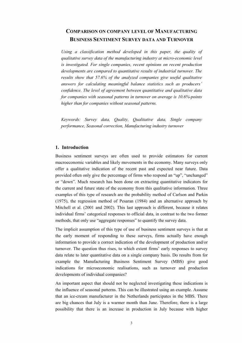
COMPARISON ON COMPANY LEVEL OF MANUFACTURING

BUSINESS SENTIMENT SURVEY DATA AND TURNOVER

Using a classification method developed in this paper, the quality of qualitative survey data of the manufacturing industry at micro-economic level is investigated. For single companies, recent opinions on recent production developments are compared to quantitative results of industrial turnover. The results show that 57.6% of the analyzed companies give useful qualitative answers for calculating meaningful balance statistics such as producers’ confidence. The level of agreement between quantitative and qualitative data for companies with seasonal patterns in turnover on average is 10.6%-points higher than for companies without seasonal patterns.

Keywords: Survey data, Quality, Qualitative data, Single company performance, Seasonal correction, Manufacturing industry turnover

1. Introduction

Business sentiment surveys are often used to provide estimators for current macroeconomic variables and likely movements in the economy. Many surveys only offer a qualitative indication of the recent past and expected near future. Data provided often only give the percentage of firms who respond an “up”, “unchanged” or “down”. Much research has been done on extracting quantitative indicators for the current and future state of the economy from this qualitative information. Three examples of this type of research are the probability method of Carlson and Parkin (1975), the regression method of Pesaran (1984) and an alternative approach by Mitchell et al. (2001 and 2002). This last approach is different, because it relates individual firms’ categorical responses to official data, in contrast to the two former methods, that only use “aggregate responses” to quantify the survey data.

The implicit assumption of this type of use of business sentiment surveys is that at the early moment of responding to these surveys, firms actually have enough information to provide a correct indication of the development of production and/or turnover. The question thus rises, to which extent firms’ early responses to survey data relate to later quantitative data on a single company basis. Do results from for example the Manufacturing Business Sentiment Survey (MBS) give good indications for microeconomic realisations, such as turnover and production developments of individual companies?

An important aspect that should not be neglected investigating these indications is the influence of seasonal patterns. This can be illustrated using an example. Assume that an ice-cream manufacturer in the Netherlands participates in the MBS. There are big chances that July is a warmer month than June. Therefore, there is a large possibility that there is an increase in production in July because with higher

4

temperatures, generally more ice-cream is sold. The manufacturer knows this beforehand, and it is relatively easy to correctly answer a qualitative question of the MBS regarding the direction of production developments. Every year this situation is the same. Thus, seasonal patterns matter because they increase the agreement between the MBS and turnover, i.e. they influence the ‘predictive power’ of the MBS.

In this paper, the quality of the MBS is examined by linking and comparing on company level MBS and industrial turnover data. A distinction is made between companies with and without seasonal patterns in turnover. This makes it possible to gauge the amount of influence of seasonality on the results.

The paper is organised as follows. In chapter 2 the linking process of the survey data with turnover is described. In chapter 3 a classification is developed with categories describing the degree to which surveys provide answers that are in accordance to turnover developments. Next, in chapter 4 and chapter 5 results for applying this classification for two questions of the MBS using not seasonally adjusted turnover are presented. In chapter 6 details and results of the procedure used to adjust turnover of individual companies for trading day and seasonal effects are described.1

The influence of seasonal patterns in turnover on results of the classification of single companies is discussed in chapter 7. Finally, conclusions and some final remarks are given in chapter 8.

1 Only turnover data has been corrected for seasonal effects, because the trichotomic nature of the answer categories of question 1 of the MBS makes a seasonal correction (very) difficult.

5

2. Data used

In this chapter, the data set used is presented. First, in section 2.1 information on the data sources for turnover and MBS are given and the linking process is described. Next, in section 2.2 differences in survey process and timeliness are discussed.

2.1 Data sources and coupling process

For the results of this paper two sources of data were used. The first source is the MBS database, which contains data of individual companies. Each company is classified into a NACE 4-digit level and a size class (5-9)2. Data available in the system at the 17th of March 2004 have been used for the calculations made in this paper. This corresponds to the months 200101 up to and including 200312. The second source is the statistic on Industrial Turnover. Two sources are available: an ‘old’ database, which contains figures from 199301 up to and including 200303, and a ‘new’ database, with figures from 200304 and later.

The MBS provides answers of individual companies, characterized by a WEID code, to (among others) the following two questions. Question 1 is “Last month’s production level (not taking the influence of holidays into account) has…”, with answer categories “increased” (1), “remained the same” (2) and “decreased” (3). And question 2 is “The average production level over the next three months (not taking the influence of holidays into account) will…” “increase” (1), “remain the same” (2) and “decrease”. The statistic on Industrial Turnover provides turnover data of individual companies, characterized by a BEID code. For each value of turnover, there is an additional variable available, which indicates if this value has been estimated or not, e.g. to cope with non-response. At company level, 10% of the turnover values have been estimated.

Using a linking scheme from WEID to BEID for the Business Survey data it is possible to link this data to the turnover data. However, for the business survey period of 200101 until 200311, 9 BEIDS (out of 1861) have more than 1 WEID in at least one period. The WEID/BEID relation is not necessarily one-to-one. This problem was overcome by just leaving these 9 BEIDs out of the linking process. Additionally, for 59 BEIDs of the MBS there is no turnover information available. The result is that for 1793 BEIDS there is at least 1 value for turnover available in the period of 199901 up to and including 200311.

For 1000 BEIDs corrections for seasonal patterns of turnover have been made. For these adjustments, turnover data for the period 199301 up to and including 200311 have been used.

2 Companies with 20 to 50, 50 to 100, 100 to 200, 200 to 500 and more than 500 employees, are classified as size class 5, 6, 7, 8, 9, respectively.

6

2.2 Difference in survey process and timeliness

For first publication industrial turnover is surveyed between t+0 and t+28 (approximately) after the end of the period under review, with approximately 65% response (weighted, average over many years) for the first estimate (Van der Stegen, 2004). At t=60, and t=90 the response is approximately 83% and 88%, respectively.

For MBS data, first, it is important to note that the way the MBS questionnaire is surveyed is different compared with the method mainly used for other statistics. A ‘time shift of one month’ is introduced. Define the coming month containing the days t..t+28/30/31 as month M. Now, what is called the ‘questionnaire of month M’is sent out to the participating companies at around t-1. Answers are collected between t+0 and t+24. The (not weighted) response to the questionnaire is approximately 90% for the final estimate. To illustrate with more detail the difference in terminology between the surveying of the MBS and turnover, an example is provided in Figure 1.

March

MBS of the month May

Turnover of referencemonth April

April May

Month

Monthly developmentSurveyed as month

March

MBS of the month May

Turnover of referencemonth April

April May

Month

Monthly developmentSurveyed as month

Figure 1. Example of the difference in surveying terminology for question 1 of the MBS and turnover data.

In this figure the three months March, April and May are considered. For the MBS the answers to the question ‘Last month’s production level (not taking the influence of holidays into account) has…’ for the ‘questionnaire of the month May’ are by definition labelled as May and also stored in the MBS database under the month May. But, according to the phrasing of the question, the respondents for the ‘questionnaire of the month May’ give answers regarding the development of the production level of April compared to March. This fact has to be kept in mind during the whole remainder of this paper. As said earlier, a time shift of one month is introduced.

For the turnover statistic, turnover of ‘reference period’ April is surveyed in May, but stored at April in the turnover database. Thus, the monthly turnover development of April can be calculated straightforward by relating the turnover value of April to the turnover value of March. No time shift is introduced.

The final conclusion is that effectively, the qualitative result of production development of April compared to March of the MBS is usually published around

7

two weeks earlier than the results of the turnover development of April compared with March. However, for a theoretical successful comparison, values of question 1 of the MBS for a certain month have to be compared to turnover developments of one month earlier.

8

3. Classification of individual companies

In this chapter, a start is made to analyse the relation between MBS and turnover data. A classification system for individual companies is developed. First, in section 3.1 an assumption for the time shift between MBS and turnover data is discussed. After this, in section 3.2 cases for companies with “logically ordered” answer categories are presented. In section 3.3 cases of companies without “logically ordered” answer categories are given. The total classification consists of 31 groups. This is too much to do analysis and interpret results. Therefore, in section 3.4, the number of groups is reduced by merging. An optimal number of data points needed to classify a company in a certain category is determined in section 3.5. Finally, in section 3.6 the number of classification categories is reduced further to a more practical classification inspired by the producers’ confidence indicator.

3.1 Time shift of question 1 of the MBS in relation to turnover data

In order to be able to compare question 1 of the MBS to turnover data3 it is necessary to have information on the relation between these two statistics (see also section 2.2). It is important to know to which month of the turnover data the MBS relates the best. The easiest way to obtain this information is to look at the way how question 1 of the MBS has been put into words: “Last month’s production level (not taking the influence of holidays into account) has…”. In this formulation, clearly the term ‘last month’s’ is used. Thus, to make a start with the research, it is logical to assume that the persons who answer to the MBS give answers that correspond to the phrasing of the question, i.e. to ‘last month’. Thus that, for example, the MBS of May relates best to the monthly turnover development of April. The appropriateness of this time shift is validated in section 4.4.

3.2 Companies with “logically ordered” answer categories

In this section the relationship between turnover and the three response categories of question 1 is analysed at company level. To make a comparison between business survey data and turnover, for each company the absolute monthly development,

tBEIDamdT , , of turnover, T , is calculated:

1,,, −−= tBEIDtBEIDtBEID TTamdT

According to the assumption made in section 3.1, it seems logical to examine if for each company the answers to question 1 are consistent with the absolute monthly

3 Strictly speaking, question 1 of the MBS should be compared with production data. However, production data are generally not available at company level. For this reason, turnover is used as a proxy for production. Doing this, it is assumed that monthly inventory changes and price developments are relatively small. The proxy may also be less accurate in branches of industry where instalments take place.

9

developments of turnover of one month earlier, 1, −tBEIDamdT . This means, that if

category 1 (“increased”), 2 (“remained the same”) or 3 (“decreased”) is answered,

1, −tBEIDamdT is larger than zero, zero (or in some interval around zero) or smaller

than zero, respectively. For analysis, an average 1, −tBEIDamdT value is calculated for

each response category 1, 2 and 3. For each time t a company answers “increased” (1) to question 1 of the MBS, all values of 1, −tBEIDamdT belonging to these

“increased”’s are averaged to BEIDamdT1 . The same is done for response categories

2 and 3, resulting in BEIDamdT 2 and BEIDamdT3 , respectively.

A logical relationship between BEIDamdT1 , BEIDamdT 2 and BEIDamdT3 can be expected. Suppose that a more optimistic answer to question 1 corresponds to a

higher value of 1, −tBEIDamdT . Then it can be expected that BEIDamdT1 >

BEIDamdT 2 , because BEIDamdT1 consists of averages of 1, −tBEIDamdT for which

the company answered “increased” in the MBS and 1, −tBEIDamdT of averages of

1, −tBEIDamdT for which the company answered “remained the same”. Following this

reasoning, it would also be logical that BEIDamdT 2 > BEIDamdT3 . This situation is given in Figure 2.

Figure 2. ( 1amdT > 2amdT ), ( 2amdT > 3amdT ), 1amdT >0 and 3amdT <0, label of this case: 123_FS123_NOBIASMBS.

But there remains a question to be solved: does question 1 of a company have a bias or not?

The result for question 1 for a company can be defined positively biased if

BEIDamdT1 <0, see Figure 3 as an example.

0 Turnover

1amdT

2amdT

3amdT

MBS category 1(“increased”)

MBS category 2(“remained the same”)

MBS category 3(“decreased”)

Figure 3. Label of this c123_FS123_POSBIASM

In this case, the answer to querealisation.

Similarly, it is possible to def

is Figure 4. Finally, a possiblsee Figure 2. For further referlabel.

Fifteen other, more obscur

BEIDamdT3 have a “logical rwith images, they are, includi

3.3 Companies without “log

In section 3.2 examples for “section, a classification for noA company without “logicallwhere a more optimistic an

1, −tBEIDamdT . Then it can

BEIDamdT 2 <= BEIDamdT3 . A

Figure 5. ‘Reversed versi

( 2amdT <=

This case is called the ‘rev

( 1amdT > 2amdT ) and ( amchanged by an unchanged or s

0

1amdT

0

1amdT

2amdT

3amdT

T

T

10

ase: BS.

Figure 4. Label of this case: 123_FS123_NEGBIASMBS.

stion 1 is too optimistic compared to the proxy for the

ine a negative bias when BEIDamdT3 >0. An example

e definition for no bias is 1amdT >0 and 3amdT <0, ence in this paper, these three cases have been given a

e cases for which BEIDamdT1 , BEIDamdT 2 and

elationship” have been defined. To not flood this paper ng their label, given in Appendix A.

ically ordered” answer categories

logically ordered” answer categories are given. In this t “logically ordered answer categories” will be given.

y ordered” answer categories is defined as a company swer to question 1 corresponds to a lower value of

be expected that BEIDamdT1 <= BEIDamdT 2 and

n unbiased version of this case is given in Figure 5.

on’ of Figure 2. In this case ( 1amdT <= 2amdT ),

3amdT ), 1amdT <0 and 3amdT >0.

ersed version’ of Figure 2, because in the criterion

2dT > 3amdT ) only the ‘greater than test’ has been maller test.

2amdT

3amdT

0 T

1amdT

2amdT

3amdT

11

For 13 of the 18 cases defined in Appendix A it is possible to define a “reversed version”. These 13 cases are classified in one single group, called “other companies without logically ordered answers”.

The classification presented in this and the former section is exhaustive: if it is applied, all companies in the data set are either classified as a company with “logically ordered answer categories” or as a company with not “logically ordered answer categories”.

3.4 Simplification of the classification

The classification developed in 3.2 and 3.3 consists of 19 groups. To simplify further analysis, the number of groups is reduced to 7 by combining them into categories. The results for these categories are given in Table 1.

Table 1. Combined classification.

Type Category 123_FS123_NOBIASMBS 113_FS13_NOBIASMBS 11_NOBIASMBS 13_NOBIASMBS 1123_FS13_NOBIASMBS 2123_FS123_POSBIASMBS 3123_FS123_NEGBIASMBS 312_O1>O2_POSBIASMBS 323_O3<O2_NEGBIASMBS 313_FS13_POSBIASMBS 313_FS13_NEGBIASMBS 31_POSBIASMBS 33_NEGBIASMBS 32_QSTBIASMBS 412_O1>O2_QSTBIASMBS 523_O3<O2_QSTBIASMBS 5123_FS13_POSBIASMBS 6123_FS13_NEGBIASMBS 6“Other companies without logically ordered answers” 7

Category 1 is a group for which companies give unbiased logically ordered answers. For category 2, the answers to question 1 are unbiased and logically ordered with respect to the answer categories “increased” and “decreased”, but “remained the same” is not ordered logically. Category 3 is a group of companies for which the response is biased, but logically ordered. Category 4 is the group of companies which always answer “remained the same” to question 1 the MBS, with unknown bias. Category 5 is a group where companies give logical ordered answers, but the bias is not known. Category 6 contains all companies with biased and “logically ordered answers” with respect to the answer categories “increased” and “decreased”, but the “remained the same” category is not ordered logically. Category 7 is the last category, containing all companies without “logically ordered answers”.

12

3.5 Number of points per company needed for classification

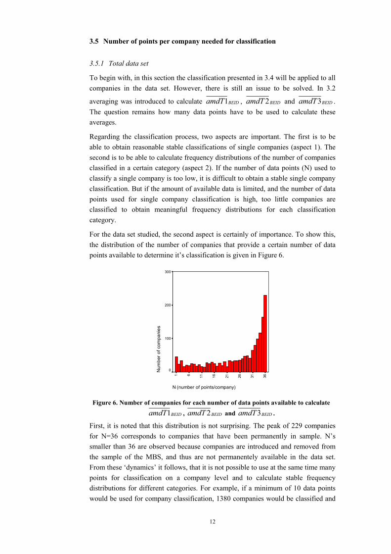
3.5.1 Total data set

To begin with, in this section the classification presented in 3.4 will be applied to all companies in the data set. However, there is still an issue to be solved. In 3.2

averaging was introduced to calculate BEIDamdT1 , BEIDamdT 2 and BEIDamdT3 .The question remains how many data points have to be used to calculate these averages.

Regarding the classification process, two aspects are important. The first is to be able to obtain reasonable stable classifications of single companies (aspect 1). The second is to be able to calculate frequency distributions of the number of companies classified in a certain category (aspect 2). If the number of data points (N) used to classify a single company is too low, it is difficult to obtain a stable single company classification. But if the amount of available data is limited, and the number of data points used for single company classification is high, too little companies are classified to obtain meaningful frequency distributions for each classification category.

For the data set studied, the second aspect is certainly of importance. To show this, the distribution of the number of companies that provide a certain number of data points available to determine it’s classification is given in Figure 6.

N (number of points/company)

36312621161161

Num

bero

fcom

pani

es

300

200

100

0

Figure 6. Number of companies for each number of data points available to calculate

BEIDamdT1 , BEIDamdT 2 and BEIDamdT3 .

First, it is noted that this distribution is not surprising. The peak of 229 companies for N=36 corresponds to companies that have been permanently in sample. N’s smaller than 36 are observed because companies are introduced and removed from the sample of the MBS, and thus are not permanentely available in the data set. From these ‘dynamics’ it follows, that it is not possible to use at the same time many points for classification on a company level and to calculate stable frequency distributions for different categories. For example, if a minimum of 10 data points would be used for company classification, 1380 companies would be classified and

13

could be used for the calculation of frequency distributions of the different categories. However, if 36 points would be used for single company classification, only 229 companies could be used to calculate these distributions. This reasoning implies that there is a quality trade-off between the classification of single companies and frequency distributions of categories.

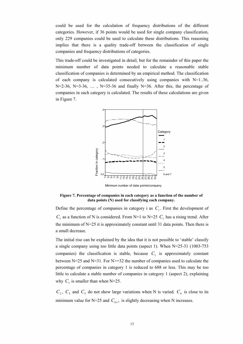
This trade-off could be investigated in detail, but for the remainder of this paper the minimum number of data points needed to calculate a reasonable stable classification of companies is determined by an empirical method. The classification of each company is calculated consecutively using companies with N=1..36, N=2-36, N=3-36, … , N=35-36 and finally N=36. After this, the percentage of companies in each category is calculated. The results of these calculations are given in Figure 7.

Minimum number of data points/company

33312927252321191715131197531

Frac

tion

inca

tego

ry

,4

,3

,2

,1

0,0

Category

1

2

3

4

5

6 and 7

Figure 7. Percentage of companies in each category as a function of the number of data points (N) used for classifying each company.

Define the percentage of companies in category i as iC . First the development of

1C as a function of N is considered. From N=1 to N=25 1C has a rising trend. After

the minimum of N=25 it is approximately constant until 31 data points. Then there is a small decrease.

The initial rise can be explained by the idea that it is not possible to ‘stable’ classify a single company using too little data points (aspect 1). When N=25-31 (1003-753 companies) the classification is stable, because 1C is approximately constant

between N=25 and N=31. For N>=32 the number of companies used to calculate the percentage of companies in category 1 is reduced to 688 or less. This may be too little to calculate a stable number of companies in category 1 (aspect 2), explaining why 1C is smaller than when N=25.

2C , 3C and 5C do not show large variations when N is varied. 4C is close to its

minimum value for N=25 and 76+C is slightly decreasing when N increases.

14

From the above reasoning, and ‘tuning’ 1C empirically to its ‘optimum’ it is decided

to use at least 25 points to classify a company into one of the seven defined categories.

3.5.2 Breakdown by size class

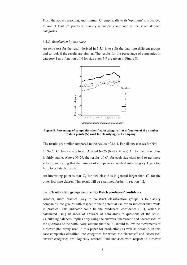
An extra test for the result derived in 3.5.1 is to split the data into different groups and to look if the results are similar. The results for the percentage of companies in category 1 as a function of N for size class 5-9 are given in Figure 8.

Minimum number of data points/company

3533312927252321191715131197531

Frac

tion

inca

tego

ry1

,5

,4

,3

,2

,1

0,0

Sizeclass

5

6

7

8

9

Figure 8. Percentage of companies classified in category 1 as a function of the number of data points (N) used for classifying each company.

The results are similar compared to the results of 3.5.1. For all size classes for N=1

to N=25 1C has a rising trend. Around N=25 (N=25±4, say) 1C for each size class

is fairly stable. Above N=29, the results of 1C for each size class tend to get more

volatile, indicating that the number of companies classified into category 1 gets too little to get stable results.

An interesting point is that 1C for size class 8 is in general larger than 1C for the

other four size classes. This result will be examined further in section 4.2.

3.6 Classification groups inspired by Dutch producers’ confidence

Another, more practical way to construct classification groups is to classify companies into groups with respect to their potential use for an indicator that exists in practice. This indicator could be the producers’ confidence (PC), which is calculated using balances of answers of companies to questions of the MBS. Calculating balances implies only using the answers “increased” and “decreased” of the questions of the MBS. Now, assume that the PC should follow the movements of turnover (the proxy used in this paper for production) as well as possible. In this case companies classified into categories for which the “increase” and “decrease” answer categories are “logically ordered” and unbiased with respect to turnover

15

should be used for calculating the PC. From this point of view, category 1 can always be used, because it has “logically ordered answer categories” without bias. This category is labelled group A. Category 3 could be used for the PC if the bias of the answers of companies can be corrected4. The combination of categories 1 and 3 is labelled group B. Categories 2 and 6 have “logically ordered answer categories” with respect to the answer categories “increased” and “decreased”, but the “remained the same” category is not ordered logically. Companies in category 2 do not have a bias; companies of category 6 could be used for the producers’ confidence if the bias of the answers could be corrected. Finally, the combination of categories 1, 2, 3 and 6 is labelled group C. As a summary, the definition of the three groups is given in Table 2.

Table 2. Groups inspired by the producers’ confidence.

Category Group 1 A1+3 B 1+2+3+6 C

4 This is a bias correction on single company level. For the Dutch producers’ confidence, an adjustment is made for bias at the aggregate level of total manufacturing industry.

16

4. Analysis of results of classifying companies using question 1

In this chapter results of classifying companies using question 1 of the MBS are presented. First, results for the classification of all companies without a breakdown to size class or NACE 2-digit level is given in section 4.1. Next, results with breakdowns into size class and NACE 2-digit level are given in sections 4.2 and 4.3, respectively. Finally, in section 4.4, the assumption made on the size of the time shift between question 1 of the MBS and turnover data (see section 3.1) is checked.

4.1 Total

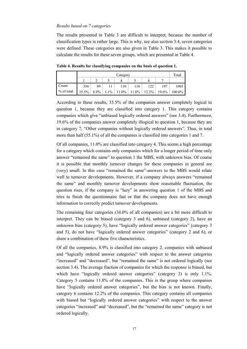
To get a first impression of the distribution of the different companies over the different classification types which have been defined in section 3.2 and 3.3, the results of applying the classification to question 1 of the data set are given in Table 3.

Table 3. Results of applying the classification to question 1.

Type Percentage Category123_FS123_NOBIASMBS 35.5 113_FS13_NOBIASMBS - 11_NOBIASMBS - 13_NOBIASMBS - 1123_FS13_NOBIASMBS 8.9 2123_FS123_POSBIASMBS 0.4 3123_FS123_NEGBIASMBS 0.5 312_O1>O2_POSBIASMBS 0.2 323_O3<O2_NEGBIASMBS - 313_FS13_POSBIASMBS - 313_FS13_NEGBIASMBS - 31_POSBIASMBS - 33_NEGBIASMBS - 32_QSTBIASMBS 11.0 412_O1>O2_QSTBIASMBS 4.5 523_O3<O2_QSTBIASMBS 7.3 5123_FS13_POSBIASMBS 5.6 6123_FS13_NEGBIASMBS 6.6 6“Other companies without logically ordered answers” 19.6 7

Strikingly, there are eight classification types into which not a single company is classified. Thinking a bit further, this is not a very strange result. The minimum number of points used for classifying each company is 25 (see section 3.5). Over such a long period of time, most companies would respond at least one time to each of the three answer categories “increased”, “remained the same” or “decreased”. All classification types into which no companies are classified are types where there are less than three answer categories used for classifying the company.

17

Results based on 7 categories

The results presented in Table 3 are difficult to interpret, because the number of classification types is rather large. This is why, see also section 3.4, seven categories were defined. These categories are also given in Table 3. This makes it possible to calculate the results for these seven groups, which are presented in Table 4.

Table 4. Results for classifying companies on the basis of question 1.

Category Total 1 2 3 4 5 6 7

Count 356 89 11 110 118 122 197 1003% of total 35.5% 8.9% 1.1% 11.0% 11.8% 12.2% 19.6% 100.0%

According to these results, 35.5% of the companies answer completely logical to question 1, because they are classified into category 1. This category contains companies which give “unbiased logically ordered answers” (see 3.4). Furthermore, 19.6% of the companies answer completely illogical to question 1, because they are in category 7, “Other companies without logically ordered answers”. Thus, in total more than half (55.1%) of all the companies is classified into categories 1 and 7.

Of all companies, 11.0% are classified into category 4. This seems a high percentage for a category which contains only companies which for a longer period of time only answer “remained the same” to question 1 the MBS, with unknown bias. Of course it is possible that monthly turnover changes for these companies in general are (very) small. In this case “remained the same”-answers to the MBS would relate well to turnover developments. However, if a company always answers “remained the same” and monthly turnover developments show reasonable fluctuation, the question rises, if the company is “lazy” in answering question 1 of the MBS and tries to finish the questionnaire fast or that the company does not have enough information to correctly predict turnover developments.

The remaining four categories (34.0% of all companies) are a bit more difficult to interpret. They can be biased (category 3 and 6), unbiased (category 2), have an unknown bias (category 5), have “logically ordered answer categories” (category 3 and 5), do not have “logically ordered answer categories” (category 2 and 6), or share a combination of these five characteristics.

Of all the companies, 8.9% is classified into category 2, companies with unbiased and “logically ordered answer categories” with respect to the answer categories “increased” and “decreased”, but “remained the same” is not ordered logically (see section 3.4). The average fraction of companies for which the response is biased, but which have “logically ordered answer categories” (category 3) is only 1.1%. Category 5 contains 11.8% of the companies. This is the group where companies have “logically ordered answer categories”, but the bias is not known. Finally, category 6 contains 12.2% of the companies. This category contains all companies with biased but “logically ordered answer categories” with respect to the answer categories “increased” and “decreased”, but the “remained the same” category is not ordered logically.

18

Results based on classification groups inspired by Dutch producers’ confidence

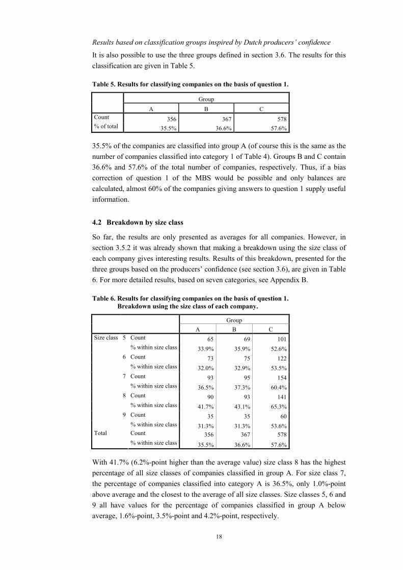
It is also possible to use the three groups defined in section 3.6. The results for this classification are given in Table 5.

Table 5. Results for classifying companies on the basis of question 1.

Group A B C

Count 356 367 578% of total 35.5% 36.6% 57.6%

35.5% of the companies are classified into group A (of course this is the same as the number of companies classified into category 1 of Table 4). Groups B and C contain 36.6% and 57.6% of the total number of companies, respectively. Thus, if a bias correction of question 1 of the MBS would be possible and only balances are calculated, almost 60% of the companies giving answers to question 1 supply useful information.

4.2 Breakdown by size class

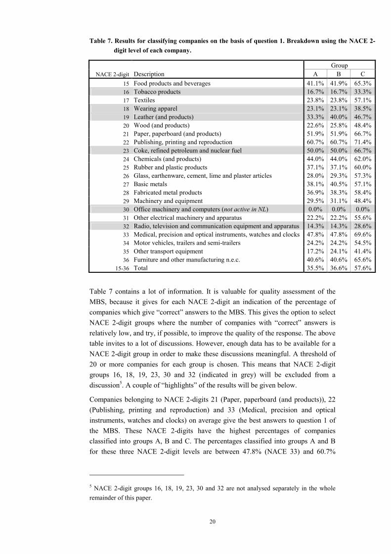
So far, the results are only presented as averages for all companies. However, in section 3.5.2 it was already shown that making a breakdown using the size class of each company gives interesting results. Results of this breakdown, presented for the three groups based on the producers’ confidence (see section 3.6), are given in Table 6. For more detailed results, based on seven categories, see Appendix B.

Table 6. Results for classifying companies on the basis of question 1. Breakdown using the size class of each company.

Group A B C

Count 65 69 1015% within size class 33.9% 35.9% 52.6%Count 73 75 1226% within size class 32.0% 32.9% 53.5%Count 93 95 1547% within size class 36.5% 37.3% 60.4%Count 90 93 1418% within size class 41.7% 43.1% 65.3%Count 35 35 60

Size class

9% within size class 31.3% 31.3% 53.6%Count 356 367 578Total % within size class 35.5% 36.6% 57.6%

With 41.7% (6.2%-point higher than the average value) size class 8 has the highest percentage of all size classes of companies classified in group A. For size class 7, the percentage of companies classified into category A is 36.5%, only 1.0%-point above average and the closest to the average of all size classes. Size classes 5, 6 and 9 all have values for the percentage of companies classified in group A below average, 1.6%-point, 3.5%-point and 4.2%-point, respectively.

19

Category B does not give much more information than category A, because the percentages of companies classified into category A and B do not differ much. The maximum difference is 2.0%-point for size class 5.

Size class 8 has, with 65.3%, also the highest percentage of companies classified into group C. A striking detail is that the percentage of companies classified into group C is higher for size class 6 than for size class 5, while for group B the percentage of size class 5 is higher than the percentage of size class 6.

These results do not support the view that smaller companies give “better” answers to question 1 of the MBS, e.g. because they have a more complete overview of the entire business. This idea has to be rejected, because classification percentages of size classes 5 and 6 are slightly lower than classification percentages op size classes 7 and 8.

The results presented in this section have to be interpreted with caution, because all percentages for different size classes are different, but relatively close to the percentage of the total without breakdown according to size classes. A first, general conclusion might be that apparently, for size classes 5 and higher, the size of the company does not practically contribute to its capacity to correctly assess the direction of turnover development at the time the MBS is held.

4.3 Breakdown by NACE 2-digit

In this section results of a breakdown by NACE 2-digit level of the classification of companies using question 1 is discussed. The breakdown in the three groups based on the producers’ confidence is presented in Table 7. For more detailed results, based on seven categories, see Appendix B.

20

Table 7. Results for classifying companies on the basis of question 1. Breakdown using the NACE 2-digit level of each company.

Group NACE 2-digit Description A B C

15 Food products and beverages 41.1% 41.9% 65.3% 16 Tobacco products 16.7% 16.7% 33.3% 17 Textiles 23.8% 23.8% 57.1% 18 Wearing apparel 23.1% 23.1% 38.5% 19 Leather (and products) 33.3% 40.0% 46.7% 20 Wood (and products) 22.6% 25.8% 48.4% 21 Paper, paperboard (and products) 51.9% 51.9% 66.7% 22 Publishing, printing and reproduction 60.7% 60.7% 71.4% 23 Coke, refined petroleum and nuclear fuel 50.0% 50.0% 66.7% 24 Chemicals (and products) 44.0% 44.0% 62.0% 25 Rubber and plastic products 37.1% 37.1% 60.0% 26 Glass, earthenware, cement, lime and plaster articles 28.0% 29.3% 57.3% 27 Basic metals 38.1% 40.5% 57.1% 28 Fabricated metal products 36.9% 38.3% 58.4% 29 Machinery and equipment 29.5% 31.1% 48.4% 30 Office machinery and computers (not active in NL) 0.0% 0.0% 0.0% 31 Other electrical machinery and apparatus 22.2% 22.2% 55.6% 32 Radio, television and communication equipment and apparatus 14.3% 14.3% 28.6% 33 Medical, precision and optical instruments, watches and clocks 47.8% 47.8% 69.6% 34 Motor vehicles, trailers and semi-trailers 24.2% 24.2% 54.5% 35 Other transport equipment 17.2% 24.1% 41.4% 36 Furniture and other manufacturing n.e.c. 40.6% 40.6% 65.6%

15-36 Total 35.5% 36.6% 57.6%

Table 7 contains a lot of information. It is valuable for quality assessment of the MBS, because it gives for each NACE 2-digit an indication of the percentage of companies which give “correct” answers to the MBS. This gives the option to select NACE 2-digit groups where the number of companies with “correct” answers is relatively low, and try, if possible, to improve the quality of the response. The above table invites to a lot of discussions. However, enough data has to be available for a NACE 2-digit group in order to make these discussions meaningful. A threshold of 20 or more companies for each group is chosen. This means that NACE 2-digit groups 16, 18, 19, 23, 30 and 32 (indicated in grey) will be excluded from a discussion5. A couple of “highlights” of the results will be given below.

Companies belonging to NACE 2-digits 21 (Paper, paperboard (and products)), 22 (Publishing, printing and reproduction) and 33 (Medical, precision and optical instruments, watches and clocks) on average give the best answers to question 1 of the MBS. These NACE 2-digits have the highest percentages of companies classified into groups A, B and C. The percentages classified into groups A and B for these three NACE 2-digit levels are between 47.8% (NACE 33) and 60.7%

5 NACE 2-digit groups 16, 18, 19, 23, 30 and 32 are not analysed separately in the whole remainder of this paper.

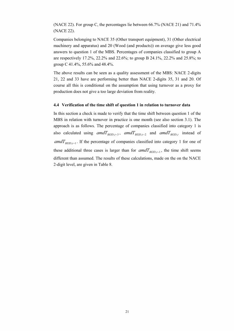
21

(NACE 22). For group C, the percentages lie between 66.7% (NACE 21) and 71.4% (NACE 22).

Companies belonging to NACE 35 (Other transport equipment), 31 (Other electrical machinery and apparatus) and 20 (Wood (and products)) on average give less good answers to question 1 of the MBS. Percentages of companies classified to group A are respectively 17.2%, 22.2% and 22.6%; to group B 24.1%, 22.2% and 25.8%; to group C 41.4%, 55.6% and 48.4%.

The above results can be seen as a quality assessment of the MBS: NACE 2-digits 21, 22 and 33 have are performing better than NACE 2-digits 35, 31 and 20. Of course all this is conditional on the assumption that using turnover as a proxy for production does not give a too large deviation from reality.

4.4 Verification of the time shift of question 1 in relation to turnover data

In this section a check is made to verify that the time shift between question 1 of the MBS in relation with turnover in practice is one month (see also section 3.1). The approach is as follows. The percentage of companies classified into category 1 is also calculated using 3, −tBEIDamdT , 2, −tBEIDamdT and tBEIDamdT , instead of

1, −tBEIDamdT . If the percentage of companies classified into category 1 for one of

these additional three cases is larger than for 1, −tBEIDamdT , the time shift seems

different than assumed. The results of these calculations, made on the on the NACE 2-digit level, are given in Table 8.

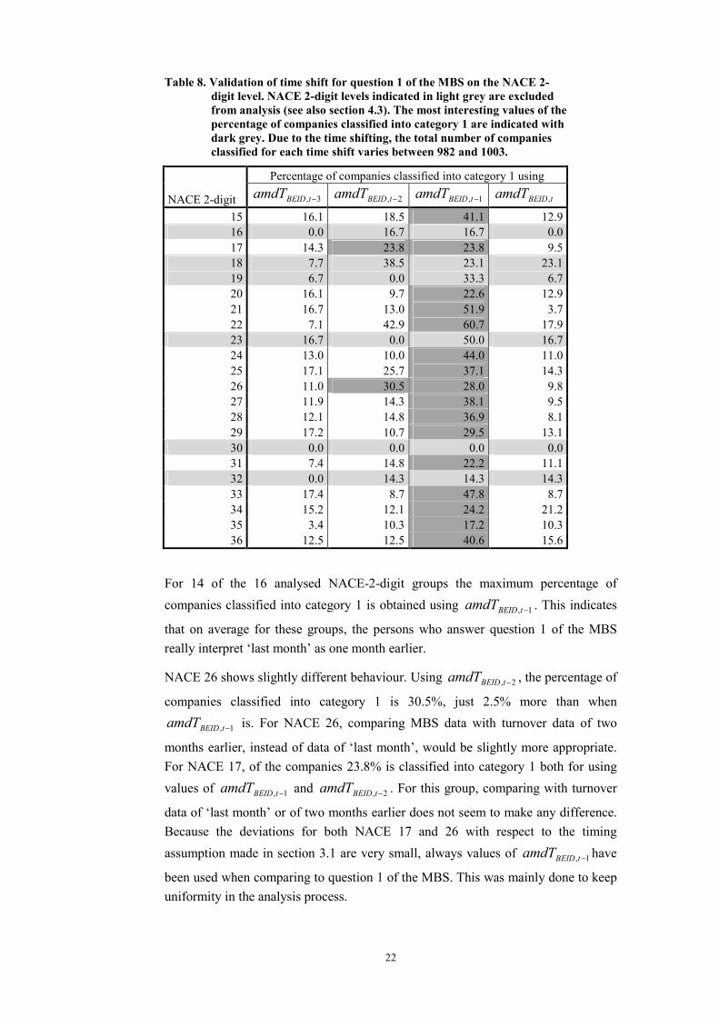
22

Table 8. Validation of time shift for question 1 of the MBS on the NACE 2-digit level. NACE 2-digit levels indicated in light grey are excluded from analysis (see also section 4.3). The most interesting values of the percentage of companies classified into category 1 are indicated with dark grey. Due to the time shifting, the total number of companies classified for each time shift varies between 982 and 1003.

Percentage of companies classified into category 1 using

NACE 2-digit 3, −tBEIDamdT 2, −tBEIDamdT 1, −tBEIDamdT tBEIDamdT ,

15 16.1 18.5 41.1 12.916 0.0 16.7 16.7 0.017 14.3 23.8 23.8 9.518 7.7 38.5 23.1 23.119 6.7 0.0 33.3 6.720 16.1 9.7 22.6 12.921 16.7 13.0 51.9 3.722 7.1 42.9 60.7 17.923 16.7 0.0 50.0 16.724 13.0 10.0 44.0 11.025 17.1 25.7 37.1 14.326 11.0 30.5 28.0 9.827 11.9 14.3 38.1 9.528 12.1 14.8 36.9 8.129 17.2 10.7 29.5 13.130 0.0 0.0 0.0 0.031 7.4 14.8 22.2 11.132 0.0 14.3 14.3 14.333 17.4 8.7 47.8 8.734 15.2 12.1 24.2 21.235 3.4 10.3 17.2 10.336 12.5 12.5 40.6 15.6

For 14 of the 16 analysed NACE-2-digit groups the maximum percentage of companies classified into category 1 is obtained using 1, −tBEIDamdT . This indicates

that on average for these groups, the persons who answer question 1 of the MBS really interpret ‘last month’ as one month earlier.

NACE 26 shows slightly different behaviour. Using 2, −tBEIDamdT , the percentage of

companies classified into category 1 is 30.5%, just 2.5% more than when

1, −tBEIDamdT is. For NACE 26, comparing MBS data with turnover data of two

months earlier, instead of data of ‘last month’, would be slightly more appropriate. For NACE 17, of the companies 23.8% is classified into category 1 both for using values of 1, −tBEIDamdT and 2, −tBEIDamdT . For this group, comparing with turnover

data of ‘last month’ or of two months earlier does not seem to make any difference. Because the deviations for both NACE 17 and 26 with respect to the timing assumption made in section 3.1 are very small, always values of 1, −tBEIDamdT have

been used when comparing to question 1 of the MBS. This was mainly done to keep uniformity in the analysis process.

23

5. Comparison between classifying using question 1 and question 2

Until now, turnover was related to the assessment of firms of “recent production” (question 1). In this chapter, question 2 on “production expectations” will also be included. In section 5.1 a view on the interpretation of question 2 of the MBS is given. Next, results of classifying companies using question 1 and question 2 are presented. A comparison without breakdown into size class or NACE 2-digit level is given in section 5.2. Results with breakdowns into size class and NACE 2-digit level are given in sections 5.3 and 5.4. Only groups A and C of the classification based on the producers’ confidence are compared. Extensive results in 7 categories with breakdowns into size class and NACE 2-digit are given in Appendix B and C. Finally, in section 5.5 a check is made if the time shift between turnover data and MBS results for question 2 is as can be expected.

5.1 Interpretation of question 2 of the MBS

Until now, only question 1 of the MBS was studied. In the remaining part of this paper, also question 2 of the MBS, “The average production level over the next three months (not taking the influence of holidays into account) will…”, is considered. The way this question will be interpreted is changed slightly compared to the interpretation suggested by the phrasing of this question. This is done because it seems unlikely that the entrepreneurs who fill in the questionnaire are able to predict turnover (benchmark for production) three months ahead in order to be capable to evaluate the expression 1,2,1,, )( −++ −++ tBEIDtBEIDtBEIDtBEID TTTTmean , the

mathematical representation of the variable asked to evaluate in the questionnaire.

In this paper, it is assumed that for question 2 the respondents in practice give answers regarding the present month, and therefore tBEIDamdT , is used as

comparison variable for question 2. It is difficult to assess whether the assumption is entirely correct or not. A very detailed investigation of the correctness of this assumption will not be discussed in this paper. Comparison tables for breakdowns into size class and NACE 2-digit level for the two different views are given in Appendix D. In general, the differences between the two methods are small6. The results may even be dependent on size class and/or NACE 2-digit level. To determine how the results of question 2 exactly have to be interpreted in practice remains a topic for future research.

6To give a quick idea: using tBEIDamdT , , for total industry, 26.6% is classified into

category 1. Using 1,2,1,, )( −++ −++ tBEIDtBEIDtBEIDtBEID TTTTmean this percentage is

27.5%, resulting in a small difference of -0.9%.

24

5.2 Total

Results for comparing results of classifying companies using question 1 and question 2 are given in Figure 9.

0%10%20%30%40%50%60%70%

A C

Group

Perc

enta

gein

grou

p

Question 1 Question 2

35,5%26,6%

57,6%46,4%

Figure 9. Comparison of classification groups A and B for question 1 and question 2.

It is obvious that it is in general more difficult to predict the future than to assess the past. For question 1, 8.9% more companies classify to group A than for question 2. For group C, this difference is 11.2%-point.

5.3 Breakdown by size class

A breakdown of the results of section 5.2 using the size class of each company is given for group A in Figure 10 and for group C in Figure 11.

0%10%20%30%40%50%60%70%

5 6 7 8 9

Sizeclass

Perc

enta

gein

grou

pA

Question 1 Question 2

Figure 10. Comparison of the percentage of companies in group A for question 1 and question 2. Breakdown by size class.

0%10%20%30%40%50%60%70%

5 6 7 8 9

Sizeclass

Perc

enta

gein

grou

pC

Question 1 Question 2

Figure 11. Comparison of the percentage of companies in group C for question 1 and question 2. Breakdown by size class.

For companies of every size class it seems more difficult to predict the future than to assess the past. However, for size class 6 the number of companies classified into group A using respectively question 1 and question 2 is, with a difference of 0.5%-point almost the same (for other size classes, this difference is at least 6.9%-point). Thus, if only results for group A are considered, for companies belonging to size class 6 prediction seems almost as easy as assessing the past.

When only group A is considered, size class 6 seems the best predicting class. However, just as in section 4.2 for question 1, the results for question 2 for different

25

size classes have to be interpreted with caution, because all percentages for different size classes are different, but relatively close to the percentage of the total without breakdown.

If group C is considered, the results would not be much different. However, for interpretation, group A may be preferable, because this group only contains “logically ordered answer categories” without bias, whereas group C also includes answers to the MBS that are not totally “logical”.

5.4 Breakdown by NACE 2-digit

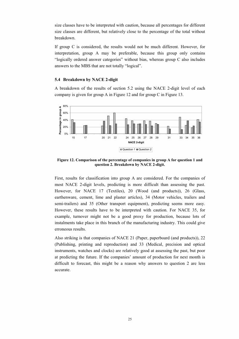
A breakdown of the results of section 5.2 using the NACE 2-digit level of each company is given for group A in Figure 12 and for group C in Figure 13.

0%

20%

40%

60%

80%

15 17 20 21 22 24 25 26 27 28 29 31 33 34 35 36

NACE 2-digit

Perc

enta

gein

grou

pA

Question 1 Question 2

Figure 12. Comparison of the percentage of companies in group A for question 1 and question 2. Breakdown by NACE 2-digit.

First, results for classification into group A are considered. For the companies of most NACE 2-digit levels, predicting is more difficult than assessing the past. However, for NACE 17 (Textiles), 20 (Wood (and products)), 26 (Glass, earthenware, cement, lime and plaster articles), 34 (Motor vehicles, trailers and semi-trailers) and 35 (Other transport equipment), predicting seems more easy. However, these results have to be interpreted with caution. For NACE 35, for example, turnover might not be a good proxy for production, because lots of instalments take place in this branch of the manufacturing industry. This could give erroneous results.

Also striking is that companies of NACE 21 (Paper, paperboard (and products)), 22 (Publishing, printing and reproduction) and 33 (Medical, precision and optical instruments, watches and clocks) are relatively good at assessing the past, but poor at predicting the future. If the companies’ amount of production for next month is difficult to forecast, this might be a reason why answers to question 2 are less accurate.

26

0%

20%

40%

60%

80%

15 17 20 21 22 24 25 26 27 28 29 31 33 34 35 36

NACE 2-digit

Perc

enta

gein

grou

pC

Question 1 Question 2

Figure 13. Comparison of the percentage of companies in group C for question 1 and question 2. Breakdown by NACE 2-digit.

If group C is considered, only NACE 20 has a higher percentage of companies classified into this group for question 2 than for question 1. Further, results for group C show similar patterns as the results for group A.

5.5 Verifying of the time shift of question 2 in relation to turnover data

In this section, the assumption made in section 5.1 that there is no time shift between question 2 and turnover developments is checked. The approach taken is the same as for question 1 described in section 4.4. The percentage of companies classified into category 1 is also calculated using 2, −tBEIDamdT , 1, −tBEIDamdT , 1, +tBEIDamdT ,

2, +tBEIDamdT , 3, +tBEIDamdT and 4, +tBEIDamdT instead of tBEIDamdT , . If the

percentage of companies classified into category 1 for one of these additional six cases is larger than for tBEIDamdT , , the time shift seems different than assumed. The

results of these calculations, made on the NACE 2-digit level, are given in Table 9.

27

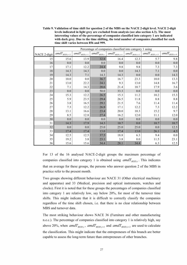
Table 9. Validation of time shift for question 2 of the MBS on the NACE 2-digit level. NACE 2-digit levels indicated in light grey are excluded from analysis (see also section 4.3). The most interesting values of the percentage of companies classified into category 1 are indicated with dark grey. Due to the time shifting, the total number of companies classified for each time shift varies between 856 and 999.

Percentage of companies classified into category 1 using

NACE 2-digit 2, −tBEIDamdT 1, −tBEIDamdT tBEIDamdT , 1, +tBEIDamdT 2, +tBEIDamdT 3, +tBEIDamdT 4, +tBEIDamdT

15 15.6 13.9 32.8 16.4 12.3 5.7 9.816 0.0 0.0 0.0 0.0 0.0 0.0 0.017 17.1 12.2 24.4 9.8 9.8 7.3 7.318 14.3 14.3 0.0 0.0 14.3 7.1 0.019 14.3 7.1 14.3 14.3 0.0 0.0 14.320 10.0 0.0 36.7 16.7 23.3 10.0 13.321 13.0 22.2 24.1 9.3 13.0 14.8 16.722 7.1 14.3 28.6 21.4 10.7 17.9 3.623 0.0 0.0 50.0 33.3 0.0 0.0 0.024 15.3 12.2 26.5 15.3 11.2 10.2 15.325 5.9 23.5 29.4 26.5 11.8 8.8 8.826 3.8 16.5 29.1 21.5 7.6 11.4 11.427 7.3 12.2 26.8 17.1 12.2 7.3 12.228 13.1 16.6 23.4 20.0 10.3 15.2 9.729 8.5 12.8 27.4 16.2 12.0 11.1 12.030 0.0 0.0 0.0 0.0 0.0 0.0 0.031 14.3 17.9 14.3 10.7 0.0 10.7 10.732 0.0 0.0 25.0 25.0 25.0 0.0 12.533 17.4 17.4 13.0 17.4 13.0 26.1 4.334 12.5 12.5 37.5 18.8 6.3 9.4 0.035 19.2 3.8 23.1 3.8 0.0 11.5 23.136 15.6 15.6 34.4 28.1 34.4 6.3 12.5

For 13 of the 16 analysed NACE-2-digit groups the maximum percentage of companies classified into category 1 is obtained using tBEIDamdT , . This indicates

that on average for these groups, the persons who answer question 2 of the MBS in practice refer to the present month.

Two groups showing different behaviour are NACE 31 (Other electrical machinery and apparatus) and 33 (Medical, precision and optical instruments, watches and clocks). First it is noted that for these groups the percentages of companies classified into category 1 are relatively low, say below 20%, for most of the turnover time shifts. This might indicate that it is difficult to correctly classify the companies regardless of the time shift chosen, i.e. that there is no clear relationship between MBS and turnover data.

The most striking behaviour shows NACE 36 (Furniture and other manufacturing n.e.c.). The percentage of companies classified into category 1 is relatively high, say above 20%, when tBEIDamdT , , 1, +tBEIDamdT

and 2, +tBEIDamdT are used to calculate

the classification. This might indicate that the entrepreneurs of this branch are better capable to assess the long-term future than entrepreneurs of other branches.

28

6. Seasonal adjustment of turnover on the company level

In the remainder of this paper the influence of companies with and without seasonal patterns in turnover on results presented earlier will be examined separately. To do this, seasonality in single company turnover has to be analyzed. The procedure used for adjusting turnover of 1000 individual companies for trading day and seasonal effects is described in section 6.1. The criterion used to decide if turnover of a company has an identifiable seasonal pattern is discussed in section 6.2. Finally, in section 6.3, the results are given.

6.1 Approach

In this section the procedure used for adjusting turnover for trading day and seasonal effects is described. The goal was to adjust turnover data of the 1003 companies analysed in chapter 4. Turnover data for period 199301 up to and including 200311 have been used. For 733 of the 1003 companies, all 133 data points were available (around 10% of these values has been estimated because of non response). For 96% of all companies 60 data points or more were available. These figures indicate that the length of turnover time series was sufficient to perform seasonal adjustment. Because data of many companies had to be processed the choice was made to use a semi-automatic procedure. This may not give the best possible seasonal adjustment for each time series, but opens the possibility to adjust the large amount of data. The final quality of the adjustments proved to be good enough for the analysis carried out in the remainder of this paper.

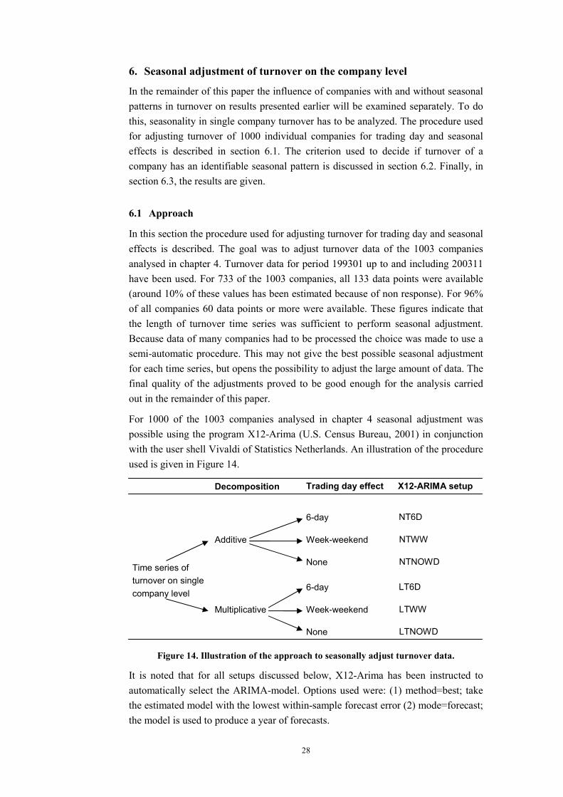
For 1000 of the 1003 companies analysed in chapter 4 seasonal adjustment was possible using the program X12-Arima (U.S. Census Bureau, 2001) in conjunction with the user shell Vivaldi of Statistics Netherlands. An illustration of the procedure used is given in Figure 14.

Figure 14. Illustration of the approach to seasonally adjust turnover data.

It is noted that for all setups discussed below, X12-Arima has been instructed to automatically select the ARIMA-model. Options used were: (1) method=best; take the estimated model with the lowest within-sample forecast error (2) mode=forecast; the model is used to produce a year of forecasts.

Time series of turnover on single company level

Additive

Multiplicative

6-day

Decomposition Trading day effect X12-ARIMA setup

NT6D

Week-weekend

None

NTWW

NTNOWD

6-day

Week-weekend

None

LT6D

LTWW

LTNOWD

29

First, the type of decomposition has been determined for each of the 1000 series. Two main types of decomposition can be performed: additive or multiplicative. The type of decomposition has been selected using an automatic method: X12-Arima performs an automatic analysis and decides which transformation to use. The setup named AOFM used for this first step is given in Appendix E.

Given the decomposition for each series it was possible to pre-process the series by correcting for possible trading day patterns using regression variables. Each company was classified as having (1) a 6-day pattern, (2) a week-weekend pattern or (3) no trading day pattern. For statistical testing a 5% significance level was used. If both the 6-day and the week-weekend pattern were significant, the method with the lowest P-value was selected.

After pre-processing, the actual seasonal adjustment has been carried out using X12-Arima. For all setups the default for the filter has been set by using the Moving Seasonality Ratio (MSR). This means that the final seasonal filter was chosen automatically. The lower and upper sigma limits used to downweight extreme irregular values in the internal seasonal adjustment procedure were set to 1.20 and 2.00, respectively. The six setups named NT6D, NTWW, NTNOWD, LT6D, LTWW and LTNOWD used for this step are given in Appendix E.

Final remark

Leap year effects were only significant for 2% of the companies analysed. In order to limit the number of X12-Arima setups needed to seasonally adjust turnover of all 1000 companies, this correction has not been applied to any company, also not to companies for which the effect was significant. Omitting this correction is expected (almost) not to influence the aggregate final results, due to the small number of companies involved.

6.2 Identification of seasonal patterns

In this section the criterion used to assess whether the turnover of a single company has an identifiable seasonal pattern or not is discussed. The quality of a seasonal adjustment is expressed using eleven M-measures generated by X12-Arima. Four important M-measures are given in Table 10.

Table 10. Seasonal adjustment: M-measures.

Measure Description M2

The relative contribution of the irregular component to the stationary portion of the variance

M7 The amount of moving seasonality present relative to the amount of stable seasonality

M10

The size of the fluctuations in the seasonal component throughout the last three years

M11 The average linear movement in the seasonal component throughout the last three years.

The value of these measures can range from 0.0 to 3.0. Lower M-measures correspond with a better seasonal adjustment.

30

The overall quality measure of a seasonal adjustment is calculated as a weighted average of these M-measures. The definitions of Q-measures are given in Table 11.

Table 11. Seasonal adjustment: Q-measures.

Measure Description Q Overall index of the acceptability of the seasonal adjustment Q2 Q statistic computed without the M2 Quality Measure statistic

Q-measures can range from 0.0 to 3.0, with 0.0 as best performance. For both the individual M- and Q-measures values above 1.0 are best avoided. Generally, the quality of an adjustment is considered reliable if the values of the mentioned measures do not exceed 0.7.

Many subjective aspects play a role to assess if a time series has an identifiable seasonal pattern or not. Often, all the different quality measures are subjectively examined for every processed series. With 1000 series “manual inspection” is not possible. The process to determine if the series have seasonal patterns has to be automated.

This has been achieved by adopting the rule that turnover data of a single company have an identifiable seasonal pattern if M7<1 and no identifiable seasonal pattern if M7≥1. The most important reason for this choice is that M7 is the most important M-measure. It has the highest weight in the Q-values.

6.3 Results

In this section, results for seasonally adjusted turnover for the 1000 companies are summarized. First, one remaining error and one remaining warning in the output of X12-Arima are discussed. For the 1000 companies processed for one company the error: “Estimation failed to converge -- maximum function evaluations reached” was reported during the final X12-Arima run. For three companies the warning: “At least one negative value was found in one of the trend cycle estimates” was found in the output. For the four companies involved, the final seasonal adjusted results of turnover were visually inspected. No strange patterns were found. Therefore, the decision has been made to keep these results in the final data set.

Results of the number of companies for each setup are given in Table 12.

Table 12. Number of companies by setup.

Setup Decomposition Trading day Number of companies NT6D Additive 6-day 110 NTWW Additive Week-weekend 226 NTNOWD Additive None 213 LT6D Multiplicative 6-day 69 LTWW Multiplicative Week-weekend 170 LTNOWD Multiplicative None 212

Overall, 549 companies have additive and 451 have multiplicative seasonality in their turnover time series. In total, trading day correction is applied for turnover of

31

575 companies. For 396 companies the week-weekend correction has been used, for 179 companies the 6-day correction. Trading day correction was not necessary for turnover of 425 companies.

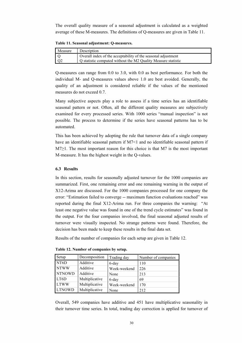
In Figure 15, a histogram of the values of M7 belonging to the turnover time series of the 1000 companies is given.

3210

M7

120

100

80

60

40

20

0

Num

bero

fcom

pani

es

Mean = 1.06Std. Dev. = 0.57N = 1,000

Figure 15. Histogram for M7.

Using the criterion M7<1 defined in section 6.2, 567 of the 1000 companies (56.7%) are identified as having a seasonal pattern in turnover. The remaining 433 companies do not have a seasonal pattern in turnover.

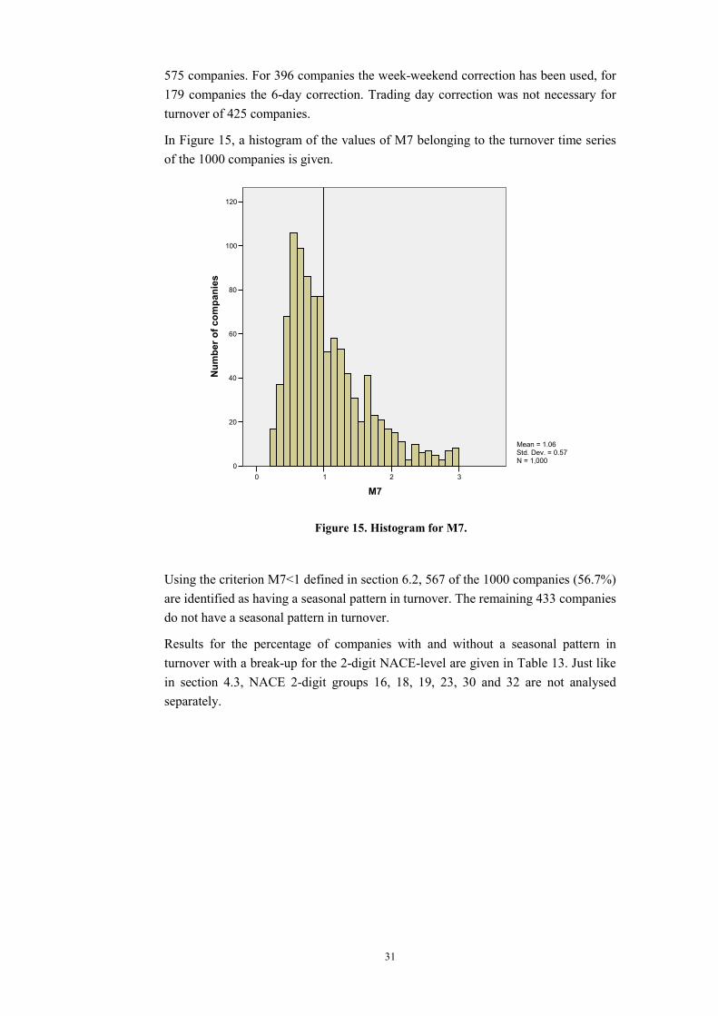
Results for the percentage of companies with and without a seasonal pattern in turnover with a break-up for the 2-digit NACE-level are given in Table 13. Just like in section 4.3, NACE 2-digit groups 16, 18, 19, 23, 30 and 32 are not analysed separately.

32

Table 13. Percentage of companies with seasonal pattern in turnover. NACE 2-digit levels indicated in grey are excluded from analysis.

Seasonal pattern? NACE 2-digit Description Yes No Total 15 Count 67 57 124 Food products and beverages

% within NACE 2-d. 54.0% 46.0% 100.0% 16 Count 3 3 6Tobacco products

% within NACE 2-d. 50.0% 50.0% 100.0% 17 Count 28 14 42 Textiles

% within NACE 2-d. 66.7% 33.3% 100.0% 18 Count 11 2 13 Wearing apparel

% within NACE 2-d. 84.6% 15.4% 100.0% 19 Count 13 2 15 Leather (and products)

% within NACE 2-d. 86.7% 13.3% 100.0% 20 Count 19 12 31 Wood (and products)

% within NACE 2-d. 61.3% 38.7% 100.0% 21 Count 38 16 54 Paper, paperboard (and products)

% within NACE 2-d. 70.4% 29.6% 100.0% 22 Count 21 7 28 Publishing, printing and reproduction

% within NACE 2-d. 75.0% 25.0% 100.0% 23 Count 0 6 6Coke, refined petroleum and nuclear

fuel % within NACE 2-d. 0.0% 100.0% 100.0% 24 Count 52 48 100 Chemicals (and products)

% within NACE 2-d. 52.0% 48.0% 100.0% 25 Count 29 6 35 Rubber and plastic products

% within NACE 2-d. 82.9% 17.1% 100.0% 26 Count 73 8 81 Glass, earthenware, cement, lime and

plaster articles % within NACE 2-d. 90.1% 9.9% 100.0% 27 Count 29 13 42 Basic metals

% within NACE 2-d. 69.0% 31.0% 100.0% 28 Count 72 77 149 Fabricated metal products

% within NACE 2-d. 48.3% 51.7% 100.0% 29 Count 38 82 120 Machinery and equipment

% within NACE 2-d. 31.7% 68.3% 100.0% 30 Count 3 0 3Office machinery and computers (not

active in NL) % within NACE 2-d. 100.0% 0.0% 100.0% 31 Count 11 16 27 Other electrical machinery and

apparatus % within NACE 2-d. 40.7% 59.3% 100.0% 32 Count 2 5 7Radio, television and communication

equipment and apparatus % within NACE 2-d. 28.6% 71.4% 100.0% 33 Count 10 13 23 Medical, precision and optical

instruments, watches and clocks % within NACE 2-d. 43.5% 56.5% 100.0% 34 Count 20 13 33 Motor vehicles, trailers and semi-

trailers % within NACE 2-d. 60.6% 39.4% 100.0% 35 Count 2 27 29 Other transport equipment

% within NACE 2-d. 6.9% 93.1% 100.0% 36 Count 26 6 32 Furniture and other manufacturing

n.e.c. % within NACE 2-d. 81.3% 18.8% 100.0% Total Count 567 433 1.000

% within NACE 2-d. 56.7% 43.3% 100.0%

33

According to Table 13, NACE 2-digit level 26 (Glass, earthenware, cement, lime and plaster articles) has with 90.1% the highest percentage of companies with a seasonal pattern in turnover, followed by NACE 25 (Rubber and plastic products) with 82.9%. Third is NACE 36 (Furniture and other manufacturing n.e.c.), with 81.3% of the companies having a seasonal pattern in turnover.

Very little seasonal influence in turnover has been found for NACE 2-digit level 35 (Other transport equipment). For only 6.9% of the companies of this branch of industry a seasonal pattern has been detected. In NACE 29 (Machinery and equipment) and 31 (Other electrical machinery and apparatus), respectively 31.7% and 40.7% of the analysed companies has an identifiable seasonal pattern in turnover.

It is noted that for NACE 23 (Coke, refined petroleum and nuclear fuel), although officially not analysed due to a lack of data, 0 out of 6 companies have a seasonal pattern in turnover. This is plausible if it is assumed that these companies use continuous production for their manufacturing process.

Taken on the whole, the results of Table 13 look plausible. They are used for the next step of this paper: assessing the influence of seasonal patterns on the percentage of companies for which turnover results agree with MBS results.

34

7. Influence of seasonal patterns on classification of companies

This chapter is an extension of section 4.3. In that section single companies were classified into groups A and C according to the correspondence between MBS and turnover data. The influence on these results of the presence or absence of seasonal patterns in turnover of these companies has not been analysed. Here, these effects are investigated. In section 7.1 a ‘subset’ method is discussed. In section 7.2 the results of a regression method are given. In section 7.3 a comparison between these two methods is made. In section 7.4 the quantitative importance of seasonality on the results for the percentage of companies classified into groups A and C is analysed. Finally, in section 7.5, the relation of the classification with the ‘predictive power’ of question 1 of the MBS is discussed.

7.1 Subset method

The objective of this section is to analyse the influence of seasonal patterns in turnover on the results for classifying companies into groups A and C. To do this, three subsets of companies and their turnover data have been created:

Subset 1: Company turnover has a seasonal pattern, but do not correct for this effect (567 companies)

Subset 2: Company turnover has a seasonal pattern, correct for this effect (567 companies)

Subset 3: Company turnover does not have a seasonal pattern (433 companies)

The idea behind this split-up is the following. In section 4.1, the percentage of companies in groups A and C has been calculated by classifying all 1003 companies as one single group. No split-up of companies dependent on the presence or absence of seasonal patterns in turnover has been made. As a result, the percentage of companies in groups A and C are based on a ‘mixture’ of companies with and without seasonal patterns. This leaves the question whether the results of section 4.1 are contaminated with seasonal patterns.

However, by making groups of companies using the defined subsets, seasonal influences can be analysed. If only subset 3 is used, the percentage of companies classified into groups A and C only relies on the 433 companies without a seasonal pattern in turnover. If only subset 1 is used, the percentage of companies classified into groups A and C is only based on the 567 companies with a seasonal pattern in turnover. Subset 2 makes it possible to analyse the percentage of the 567 companies with a seasonal pattern classified into groups A and C after turnover has been adjusted for these seasonal influences.

Thus, using the three subsets, it is possible to see how seasonal patterns in turnover influence the results presented in section 4.1. The results for classifying companies into groups A and C for the different subsets using the same method as described in section 4.1 is given in Table 14.

35

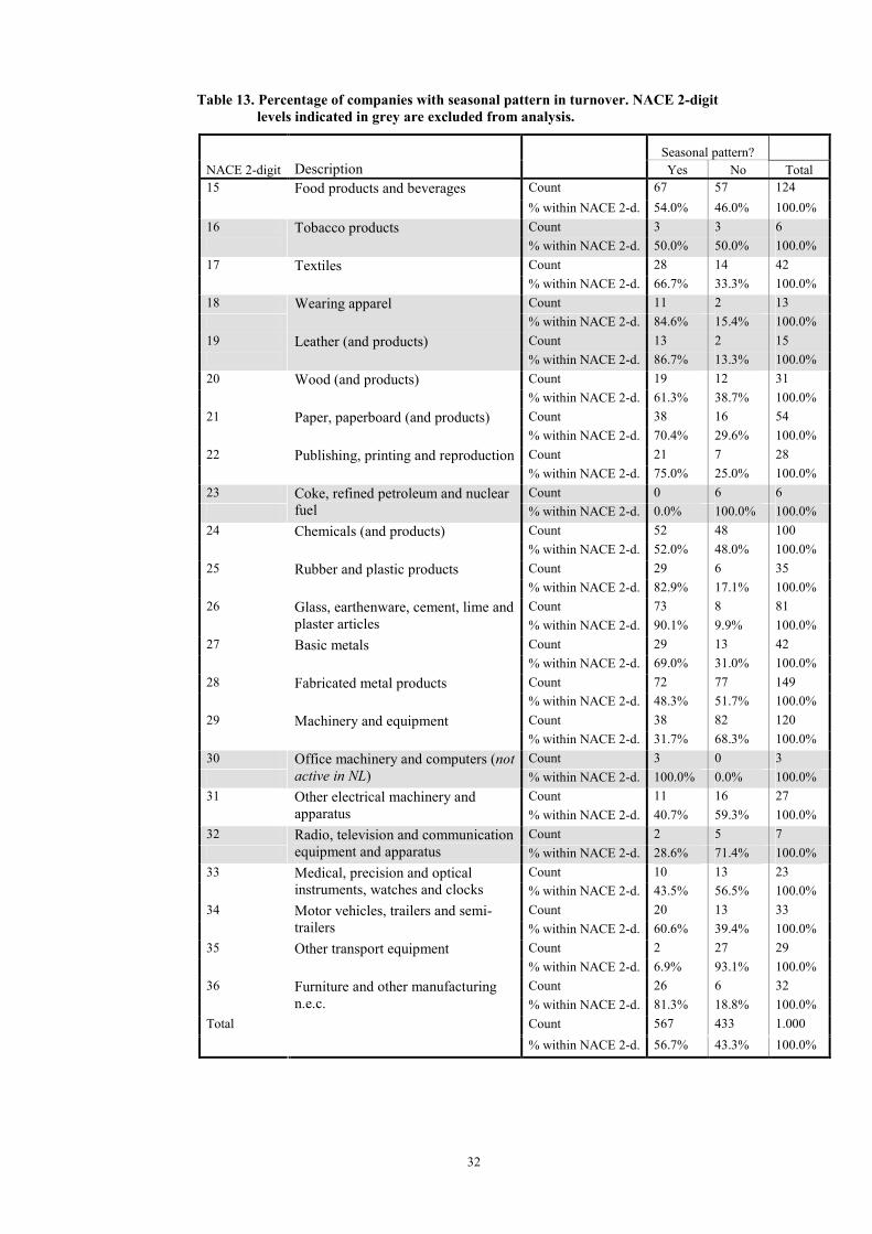
Table 14. Percentage of companies classified into group A and C, by subset.

Group A C

Section 4.1 35.5 57.6Subset 1 41.6 62.3Subset 2 27.9 50.1Subset 3 27.5 51.7

The percentage of companies classified into group A for subset 1 is 6.1% larger than the percentage of companies classified into group A in section 4.1. The same percentage for subset 3 is 8.0% smaller than for the results of section 4.1. The results for group C are similar. The percentage of companies classified into this group is 62.3% for subset 1 and 51.7% for subset 3.7 This is 4.7% higher and 5.9% lower than the results of section 4.1.

The results are not surprising. If the turnover of a company has a seasonal pattern, there is a big chance that the MBS data have a similar seasonal pattern. This automatically leads to a better agreement between MBS and turnover data compared to when this seasonal pattern would not be present.

The results of section 4.1 can also be presented as weighed averages of the results for subsets 1 and 3. The fractions of companies in each subset are used as weights.

Group A Group C

5.2710004336.41

10005675.35 ⋅+⋅= 7.51

10004333.62

10005676.57 ⋅+⋅≅

(0.1%-point round-off error)

In this way, the results of section 4.1 have been ‘decomposed’ into the two subsets. The percentage of companies classified into group A for companies with a seasonal pattern in turnover is 14.1%-point higher than for companies without a seasonal pattern. For group C the results for companies with a seasonal pattern in turnover are 10.6%-point better. Thus, accounting for seasonal effects increases the correspondence between MBS and turnover data.

The results indicate that the agreement of question 1 of the MBS with turnover developments is better for companies with seasonal patterns. This is most probably caused by common seasonal patterns between MBS and turnover data. Comparing results for subset 1, 2 and 3 (see Table 14) exemplifies this idea. For subset 1, the percentage of companies classified into group A is 41.6%. For subset 2, the seasonally adjusted version of subset 1, the percentage of companies classified into group A drops to 27.9%. This is almost equal to the 27.5% for subset 3. Thus, after 7 The percentages 62.3% and 51.7% are significantly different (χ²-test, P-value=0.001).

Subset 1 Subset 3 Subset 1 Subset 3

36

seasonal adjustment, the agreement of question 1 with single company turnover developments on average is the same for all companies.

7.2 Regression method

In this section an alternative for the subset method described in section 7.1 is given. Two data sources are used. The first source is the percentage of companies classified into groups A an C, with breakdown using the NACE 2-digit level. These data have been taken from Table 7 of section 4.3. The second data source is the percentage of companies with a seasonal pattern, also with a breakdown into NACE 2-digit level. These data have been taken from Table 13 of section 6.3. Combined data is given in Table 15. Just like in section 4.3, NACE 2-digit groups 16, 18, 19, 23, 30 and 32 are excluded from analysis because of data shortage.

Table 15. Percentage of companies with seasonal pattern in turnover and percentage of companies classified into groups A and C. Breakdown using the NACE 2-digit level of each company. NACE 2-digit levels indicated in grey are excluded from analysis.

Percentage of companies in group NACE 2-digit

Percentage of companies with seasonal pattern in turnover A C

15 54.0 41.1 65.316 50.0 16.7 33.317 66.7 23.8 57.118 84.6 23.1 38.519 86.7 33.3 46.720 61.3 22.6 48.421 70.4 51.9 66.722 75.0 60.7 71.423 0.0 50.0 66.724 52.0 44.0 62.025 82.9 37.1 60.026 90.1 28.0 57.327 69.0 38.1 57.128 48.3 36.9 58.429 31.7 29.5 48.430 100.0 0.0 0.031 40.7 22.2 55.632 28.6 14.3 28.633 43.5 47.8 69.634 60.6 24.2 54.535 6.9 17.2 41.436 81.3 40.6 65.6

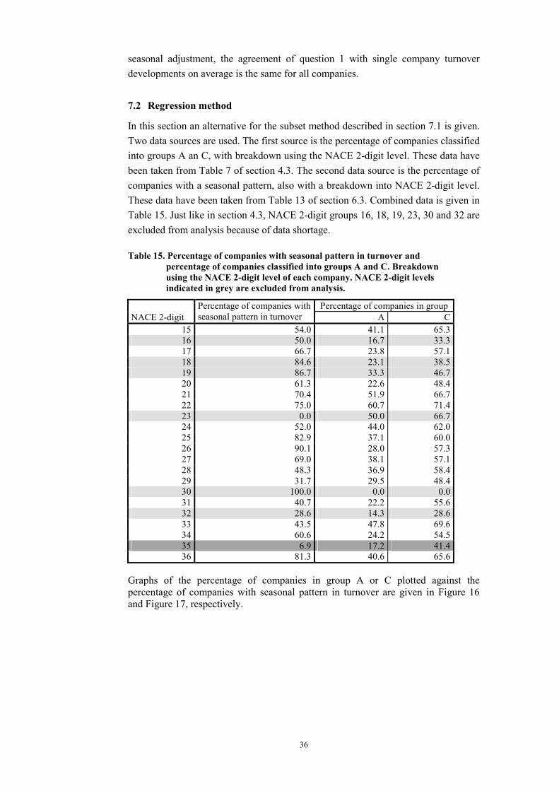
Graphs of the percentage of companies in group A or C plotted against the percentage of companies with seasonal pattern in turnover are given in Figure 16 and Figure 17, respectively.

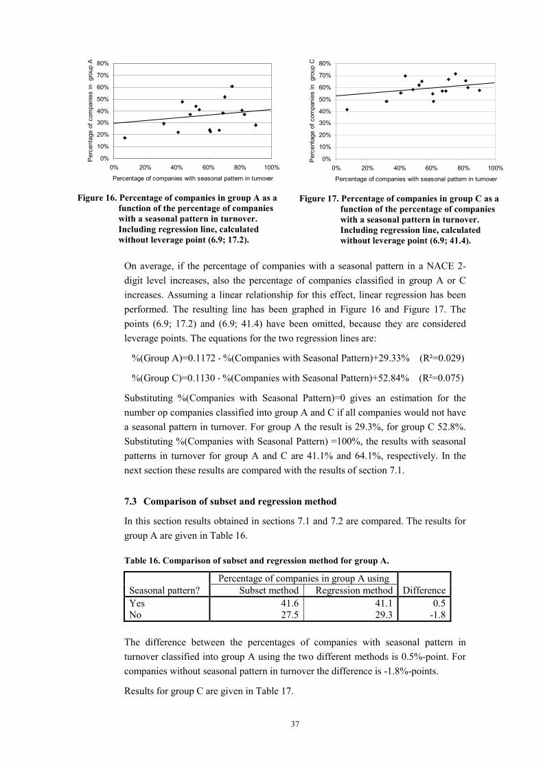
37

0%

10%

20%

30%

40%

50%

60%

70%

80%

0% 20% 40% 60% 80% 100%

Percentage of companies with seasonal pattern in turnover

Per

cent

age

ofco

mpa

nies

ingr

oup

A

Figure 16. Percentage of companies in group A as a function of the percentage of companies with a seasonal pattern in turnover. Including regression line, calculated without leverage point (6.9; 17.2).

0%

10%

20%

30%

40%

50%

60%

70%

80%

0% 20% 40% 60% 80% 100%

Percentage of companies with seasonal pattern in turnover

Per

cent

age

ofco

mpa

nies

ingr

oup

C

Figure 17. Percentage of companies in group C as a function of the percentage of companies with a seasonal pattern in turnover. Including regression line, calculated without leverage point (6.9; 41.4).

On average, if the percentage of companies with a seasonal pattern in a NACE 2-digit level increases, also the percentage of companies classified in group A or C increases. Assuming a linear relationship for this effect, linear regression has been performed. The resulting line has been graphed in Figure 16 and Figure 17. The points (6.9; 17.2) and (6.9; 41.4) have been omitted, because they are considered leverage points. The equations for the two regression lines are:

%(Group A)=0.1172 �%(Companies with Seasonal Pattern)+29.33% (R²=0.029)

%(Group C)=0.1130 �%(Companies with Seasonal Pattern)+52.84% (R²=0.075)

Substituting %(Companies with Seasonal Pattern)=0 gives an estimation for the number op companies classified into group A and C if all companies would not have a seasonal pattern in turnover. For group A the result is 29.3%, for group C 52.8%. Substituting %(Companies with Seasonal Pattern) =100%, the results with seasonal patterns in turnover for group A and C are 41.1% and 64.1%, respectively. In the next section these results are compared with the results of section 7.1.

7.3 Comparison of subset and regression method

In this section results obtained in sections 7.1 and 7.2 are compared. The results for group A are given in Table 16.

Table 16. Comparison of subset and regression method for group A.

Percentage of companies in group A using Seasonal pattern? Subset method Regression method DifferenceYes 41.6 41.1 0.5No 27.5 29.3 -1.8

The difference between the percentages of companies with seasonal pattern in turnover classified into group A using the two different methods is 0.5%-point. For companies without seasonal pattern in turnover the difference is -1.8%-points.

Results for group C are given in Table 17.

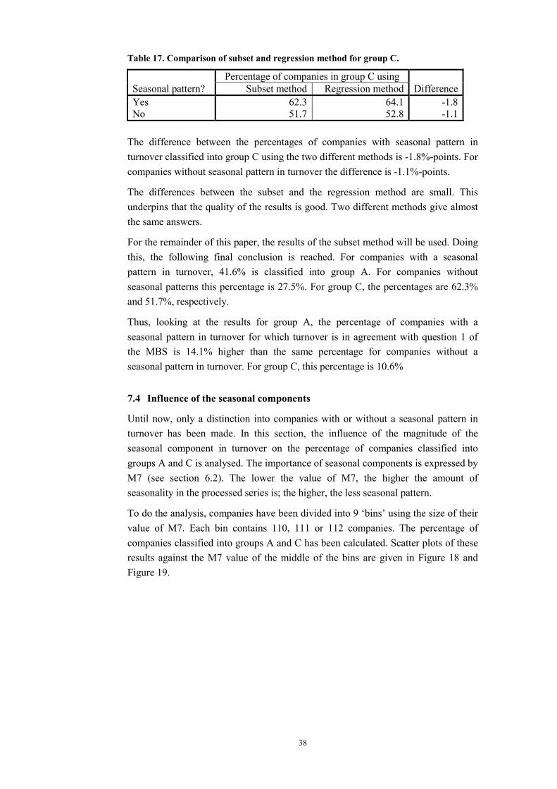
38

Table 17. Comparison of subset and regression method for group C.

Percentage of companies in group C using Seasonal pattern? Subset method Regression method DifferenceYes 62.3 64.1 -1.8No 51.7 52.8 -1.1

The difference between the percentages of companies with seasonal pattern in turnover classified into group C using the two different methods is -1.8%-points. For companies without seasonal pattern in turnover the difference is -1.1%-points.

The differences between the subset and the regression method are small. This underpins that the quality of the results is good. Two different methods give almost the same answers.

For the remainder of this paper, the results of the subset method will be used. Doing this, the following final conclusion is reached. For companies with a seasonal pattern in turnover, 41.6% is classified into group A. For companies without seasonal patterns this percentage is 27.5%. For group C, the percentages are 62.3% and 51.7%, respectively.

Thus, looking at the results for group A, the percentage of companies with a seasonal pattern in turnover for which turnover is in agreement with question 1 of the MBS is 14.1% higher than the same percentage for companies without a seasonal pattern in turnover. For group C, this percentage is 10.6%

7.4 Influence of the seasonal components

Until now, only a distinction into companies with or without a seasonal pattern in turnover has been made. In this section, the influence of the magnitude of the seasonal component in turnover on the percentage of companies classified into groups A and C is analysed. The importance of seasonal components is expressed by M7 (see section 6.2). The lower the value of M7, the higher the amount of seasonality in the processed series is; the higher, the less seasonal pattern.

To do the analysis, companies have been divided into 9 ‘bins’ using the size of their value of M7. Each bin contains 110, 111 or 112 companies. The percentage of companies classified into groups A and C has been calculated. Scatter plots of these results against the M7 value of the middle of the bins are given in Figure 18 and Figure 19.

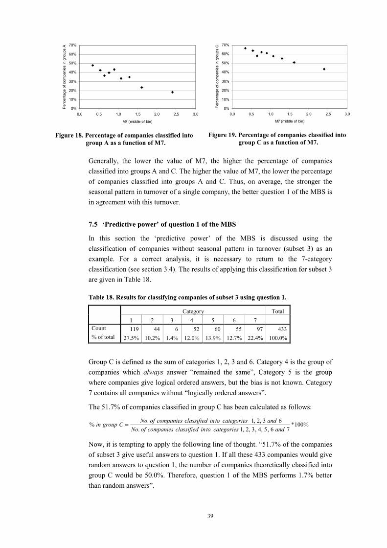
39

0%

10%

20%

30%

40%

50%

60%

70%

0,0 0,5 1,0 1,5 2,0 2,5 3,0

M7 (middle of bin)

Perc

enta

geof

com

pani

esin

grou

psA

Figure 18. Percentage of companies classified into group A as a function of M7.

0%

10%

20%

30%

40%

50%

60%

70%

0,0 0,5 1,0 1,5 2,0 2,5 3,0

M7 (middle of bin)

Perc

enta

geof

com

pani

esin

grou

psC

Figure 19. Percentage of companies classified into group C as a function of M7.

Generally, the lower the value of M7, the higher the percentage of companies classified into groups A and C. The higher the value of M7, the lower the percentage of companies classified into groups A and C. Thus, on average, the stronger the seasonal pattern in turnover of a single company, the better question 1 of the MBS is in agreement with this turnover.

7.5 ‘Predictive power’ of question 1 of the MBS

In this section the ‘predictive power’ of the MBS is discussed using the classification of companies without seasonal pattern in turnover (subset 3) as an example. For a correct analysis, it is necessary to return to the 7-category classification (see section 3.4). The results of applying this classification for subset 3 are given in Table 18.

Table 18. Results for classifying companies of subset 3 using question 1.

Category Total 1 2 3 4 5 6 7

Count 119 44 6 52 60 55 97 433% of total 27.5% 10.2% 1.4% 12.0% 13.9% 12.7% 22.4% 100.0%

Group C is defined as the sum of categories 1, 2, 3 and 6. Category 4 is the group of companies which always answer “remained the same”, Category 5 is the group where companies give logical ordered answers, but the bias is not known. Category 7 contains all companies without “logically ordered answers”.

The 51.7% of companies classified in group C has been calculated as follows:

%100*76,5,4,3,2,1.

63,2,1.%andcategoriestoinclassifiedcompaniesofNo

andcategoriestoinclassifiedcompaniesofNoCgroupin =

Now, it is tempting to apply the following line of thought. “51.7% of the companies of subset 3 give useful answers to question 1. If all these 433 companies would give random answers to question 1, the number of companies theoretically classified into group C would be 50.0%. Therefore, question 1 of the MBS performs 1.7% better than random answers”.

40

This line of thought is erroneous, because it is known that the 52 companies classified into category 4 certainly give strongly biased answers. They always answer “remained the same”, for all months studied. In section 4.1, it was even questioned if these companies are “lazy” in answering question 1 of the MBS and try to finish the questionnaire fast. These companies maybe do not try to give good indications for turnover developments. For this reason, it seems better to exclude category 4 totally from analysis when estimating the ‘predictive power’ of question 1. This leads to the following definition:

%100*76,5,3,2,1.

63,2,1.''andcategoriestoinclassifiedcompaniesofNo

andcategoriestoinclassifiedcompaniesofNopowerpredictive =

The ‘predictive power’ for different sets of companies is given in Table 19.

Table 19. ‘Predictive power’ of question 1.

‘Predictive power’Section 4.1 64.7%Subset 1 69.2%Subset 3 58.8%

For subset 3 the ‘predictive power’ is 58.8%. This is 8.8% better than random answers. For companies with a seasonal pattern in turnover (subset 1) the ‘predictive power’ is 19.2% higher than pure guesses. For the results of section 4.1 the ‘predictive power’ of question 1 is 64.7%. This is 15.7% higher than random answers.

Thus, the ‘predictive power’ of question 1 is influenced by seasonal patterns. The ‘predictive power’ of question 1 is higher when companies have seasonal patterns in turnover.

41

8. Conclusions

In this chapter, the conclusions of this paper are presented and some final remarks are given.

8.1 Conclusions

• A classification has been developed to determine to which extent the answers of individual companies to the Manufacturing Business Sentiment Survey data relate to Turnover data. This classification can be used for:

o quality assessment of MBS data on individual company level

o quantifying Business Survey data.

• Turnover data of single companies has been seasonally adjusted with a semi-automatic procedure using X12-Arima. 57% of the companies have a seasonal pattern in turnover.

• Of all classified companies, 35.5% give “logical” and unbiased answers to question 1 (“recent production”) of the MBS. For the subset of companies with a seasonal pattern in turnover this percentage is 41.6%; for the subset of companies without a seasonal pattern it is 27.5%.

• 19.6% of the companies answer completely illogical to question 1 and 11.0% answer “remained the same” for a longer period of time.

• Of all classified companies, if only balances are calculated and bias correction is applied, on average 57.6% of the companies give useful answers to question 1 of the MBS. For the subset of companies with a seasonal pattern in turnover this percentage is 62.3%; for the subset of companies without a seasonal pattern in turnover it is 51.7%.

• The level of agreement between question 1 of the MBS and turnover partly resides in seasonal patterns. On average, the stronger the seasonal pattern in turnover of a single company, the better question 1 of the MBS is in agreement with this turnover development.

• Excluding companies that always answer “remained the same” from the calculations, the ‘predictive power’ of companies with a seasonal pattern in turnover is 69.2%. For companies without a seasonal pattern in turnover, the ‘predictive power’ is 58.8%. This is respectively 19.2% and 8.8% better than if answers of companies to question 1 would be completely random.

• Of all classified companies, 26.6% give “logical” and unbiased answers to question 2 (“production expectations”) of the MBS. 27.5% of the companies answer completely illogical to question 2 and 12.6% answer “remain the same” for a longer period of time.

42

• Of all classified companies, if only balances are calculated and bias correction is applied, on average 46.6% of the companies give useful answers to question 2 of the MBS.

• The time shift in relation to turnover data of the answers to question 1 of the MBS is, in general, in agreement with the time shift that the phrasing of the question suggests. The same conclusion is drawn for question 2.

• Companies, in general, are better at assessing the recent past than predicting the near future.

8.2 Remarks

• For different size classes, it seems that the size of the company has practically no influence on its capacity to correctly assess the direction of turnover development at the time the MBS is held.

• Specific NACE 2-digit groups seem better at assessing the past than others.

• Regarding question 2 of the MBS, it is not clear if the persons answering to the MBS are capable of predicting turnover (benchmark for production) three months ahead. This topic could be investigated more in depth.

43

References

Carlson, J.A. and M. Parkin (1975), Inflation Expectations, Economica, May, 123-138.

Mitchell, James, Richard J. Smith, Martin R. Weale (2001), Quantification of Qualitative Firm-Level Survey Data, Economic Journal, 112 (478): C117-35.

Mitchell, James, Richard J. Smith, Martin R. Weale (2002), Aggregate versus Disaggregate Survey-Based Indicators of Economic Activity.

Pesaran, M.H. (1984), “Expectations formation and macroeconomic modelling”. In Contemporary Macroeconomic Modelling (Eds. Malgrange, P. and P. Muet), Blackwell, Oxford.

Stegen, R.H.M. van der (2004), Improved quality of statistics of manufacturing turnover: timeliness and accuracy, Statistics Netherlands Internal Report, Voorburg

U.S. Census Bureau, X12-Arima Reference Manual, Version 0.2.8, January 12, 2001

Appendix A. Cases

This appendix contains a description of all cases defined for the classification developed in chapter 3.

123_FS123_NOBIASMBS 123_FS123_POSBIASMBS 123_FS123_NEGBIASMBS

( 1amdT > 2amdT ) a

( 2amdT > 3amdT )

1amdT >0 and amdT

123_FS13_NOBIASM

1amdT > 3amdT

( 2amdT <= amdT2amdT >= 1amdT )

1amdT >0 and amdT

0

1amdT

2amdT

3amdT

0

1amdT2amdT

3amdT

0

amdT

2amdT3amdT

0

1amdT

0

1amdT

T T

T

nd

3 <0

( 1amdT > 2amdT ) and

( 2amdT > 3amdT )

1amdT <= 0

( 1amdT > 2amdT ) and

( 2amdT > 3amdT )

3amdT >=0

BS 123_FS13_POSBIASMBS 123_FS13_NEGBIASMBS

0

1amdT

2amdT0

1amdT1

2amdT

3amdT

2amdT

3amdT

TT

T

3amdT

0

1amdT2amdT

0

1amdT2amdT

2amdT3amdT

T

T T

44

and

3 or

3 <0

1amdT > 3amdT and

( 2amdT <= 3amdT or

2amdT >= 1amdT )

1amdT <= 0

1amdT > 3amdT and

( 2amdT <= 3amdT or

2amdT >= 1amdT )

3amdT >=0

3amdT3amdT

13_FS13_NOBIASMBS 13_FS13_POSBIASMBS 13_FS13_NEGBIASMBS

1amdT > 3amdT

1amdT >0 and

3amdT <0

1amdT > 3amdT

1amdT <= 0

1amdT > 3amdT

3amdT >=0

12_O1>O2_POSBIASMBS 12_O1>O2_QSTBIASMBS

1amdT > 2amdT

1amdT <=0

23_O3<O2_NEGBIASM

2amdT > 3amdT

3amdT >=0

0

amdT

amdT

0

1amdT

2amdT0

1amdT

0

1amdT

0

1amdT

3amdT

0

1amdT

3amdT

0

1amdT

3amdT

T T

T

T T

T

and 1amdT > 2amdT and

1amdT >0

1amdT > 2amdT and

1amdT >0

BS 23_O3<O2_QSTBIASMBS

2

02amdT

0

2amdT

2amdT 2amdT

T

T T

45

and 2amdT > 3amdT and

3amdT <0

2amdT > 3amdT and

3amdT <0

3 3amdT 3amdT

2_QSTBIASMBS

2amdT arbitrary

1_NOBIASMBS

1amdT >=0

3_NOBIASMBS

3amdT <0

0

2amdT

0

3amdT

0

2amdT

0

1amdT

02amdT

T T

T

2amdT arbitrary 2amdT arbitrary

1_POSBIASMBS

0

1amdT

T

T

1amdT <0

3_NEGBIASMBS

0 TT

T

46

3amdT >=0

3amdT

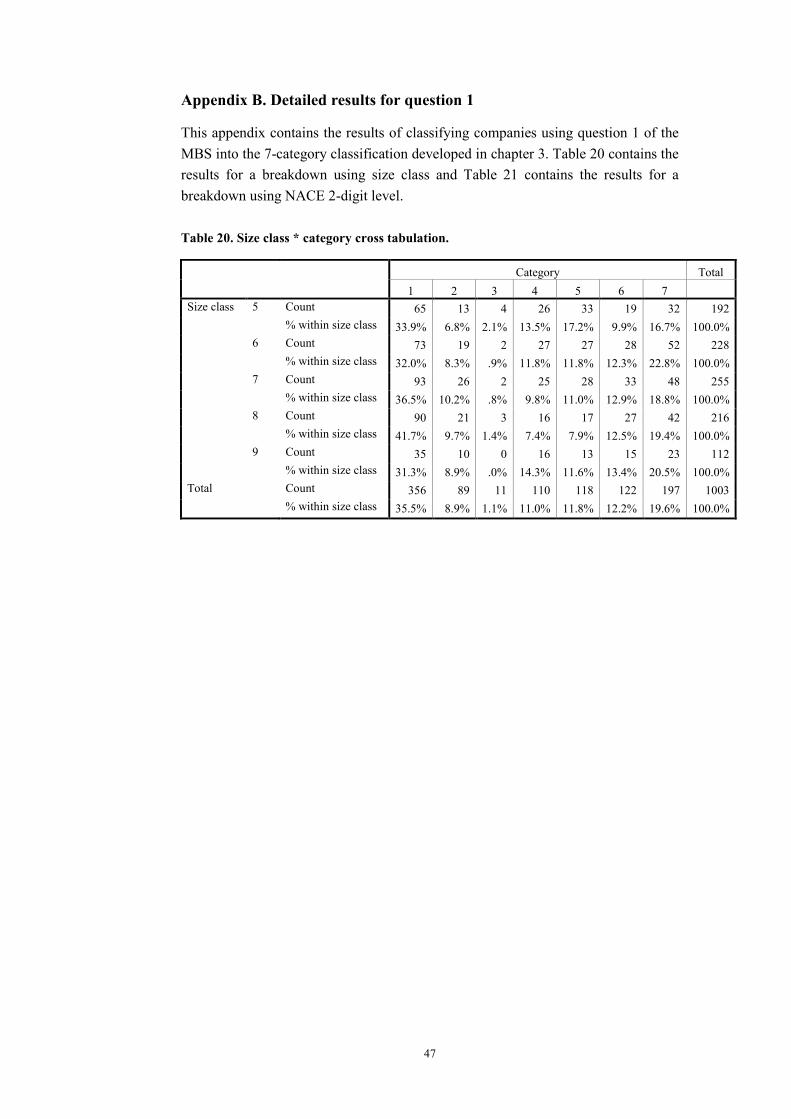
47

Appendix B. Detailed results for question 1

This appendix contains the results of classifying companies using question 1 of the MBS into the 7-category classification developed in chapter 3. Table 20 contains the results for a breakdown using size class and Table 21 contains the results for a breakdown using NACE 2-digit level.

Table 20. Size class * category cross tabulation.

Category Total 1 2 3 4 5 6 7

Size class 5 Count 65 13 4 26 33 19 32 192% within size class 33.9% 6.8% 2.1% 13.5% 17.2% 9.9% 16.7% 100.0%

6 Count 73 19 2 27 27 28 52 228% within size class 32.0% 8.3% .9% 11.8% 11.8% 12.3% 22.8% 100.0%

7 Count 93 26 2 25 28 33 48 255% within size class 36.5% 10.2% .8% 9.8% 11.0% 12.9% 18.8% 100.0%

8 Count 90 21 3 16 17 27 42 216% within size class 41.7% 9.7% 1.4% 7.4% 7.9% 12.5% 19.4% 100.0%

9 Count 35 10 0 16 13 15 23 112% within size class 31.3% 8.9% .0% 14.3% 11.6% 13.4% 20.5% 100.0%

Total Count 356 89 11 110 118 122 197 1003% within size class 35.5% 8.9% 1.1% 11.0% 11.8% 12.2% 19.6% 100.0%

48

Table 21. NACE 2-digit * category cross tabulation. Groups with less than 20 companies are indicated in grey.

Category Total 1 2 3 4 5 6 7

NACE 2-digit 15 Count 51 9 1 9 9 20 25 124% within NACE 2-d. 41.1% 7.3% .8% 7.3% 7.3% 16.1% 20.2% 100.0%

16 Count 1 0 0 1 1 1 2 6% within NACE 2-d. 16.7% .0% .0% 16.7% 16.7% 16.7% 33.3% 100.0%

17 Count 10 6 0 0 7 8 11 42% within NACE 2-d. 23.8% 14.3% .0% .0% 16.7% 19.0% 26.2% 100.0%

18 Count 3 1 0 3 2 1 3 13% within NACE 2-d. 23.1% 7.7% .0% 23.1% 15.4% 7.7% 23.1% 100.0%

19 Count 5 1 1 3 1 0 4 15% within NACE 2-d. 33.3% 6.7% 6.7% 20.0% 6.7% .0% 26.7% 100.0%

20 Count 7 3 1 3 5 4 8 31% within NACE 2-d. 22.6% 9.7% 3.2% 9.7% 16.1% 12.9% 25.8% 100.0%

21 Count 28 4 0 5 7 4 6 54% within NACE 2-d. 51.9% 7.4% .0% 9.3% 13.0% 7.4% 11.1% 100.0%

22 Count 17 3 0 0 1 0 7 28% within NACE 2-d. 60.7% 10.7% .0% .0% 3.6% .0% 25.0% 100.0%

23 Count 3 1 0 0 0 0 2 6% within NACE 2-d. 50.0% 16.7% .0% .0% .0% .0% 33.3% 100.0%

24 Count 44 8 0 13 10 10 15 100% within NACE 2-d. 44.0% 8.0% .0% 13.0% 10.0% 10.0% 15.0% 100.0%

25 Count 13 4 0 2 4 4 8 35% within NACE 2-d. 37.1% 11.4% .0% 5.7% 11.4% 11.4% 22.9% 100.0%

26 Count 23 6 1 9 9 17 17 82% within NACE 2-d. 28.0% 7.3% 1.2% 11.0% 11.0% 20.7% 20.7% 100.0%

27 Count 16 3 1 6 6 4 6 42% within NACE 2-d. 38.1% 7.1% 2.4% 14.3% 14.3% 9.5% 14.3% 100.0%

28 Count 55 15 2 19 15 15 28 149% within NACE 2-d. 36.9% 10.1% 1.3% 12.8% 10.1% 10.1% 18.8% 100.0%

29 Count 36 8 2 17 24 13 22 122% within NACE 2-d. 29.5% 6.6% 1.6% 13.9% 19.7% 10.7% 18.0% 100.0%

30 Count 0 0 0 0 1 0 2 3% within NACE 2-d. .0% .0% .0% .0% 33.3% .0% 66.7% 100.0%

31 Count 6 2 0 4 2 7 6 27% within NACE 2-d. 22.2% 7.4% .0% 14.8% 7.4% 25.9% 22.2% 100.0%

32 Count 1 1 0 1 3 0 1 7% within NACE 2-d. 14.3% 14.3% .0% 14.3% 42.9% .0% 14.3% 100.0%

33 Count 11 3 0 1 3 2 3 23% within NACE 2-d. 47.8% 13.0% .0% 4.3% 13.0% 8.7% 13.0% 100.0%

34 Count 8 3 0 6 4 7 5 33% within NACE 2-d. 24.2% 9.1% .0% 18.2% 12.1% 21.2% 15.2% 100.0%

35 Count 5 3 2 6 2 2 9 29% within NACE 2-d. 17.2% 10.3% 6.9% 20.7% 6.9% 6.9% 31.0% 100.0%

36 Count 13 5 0 2 2 3 7 32% within NACE 2-d. 40.6% 15.6% .0% 6.3% 6.3% 9.4% 21.9% 100.0%

Total Count 356 89 11 110 118 122 197 1003% within NACE 2-d. 35.5% 8.9% 1.1% 11.0% 11.8% 12.2% 19.6% 100.0%

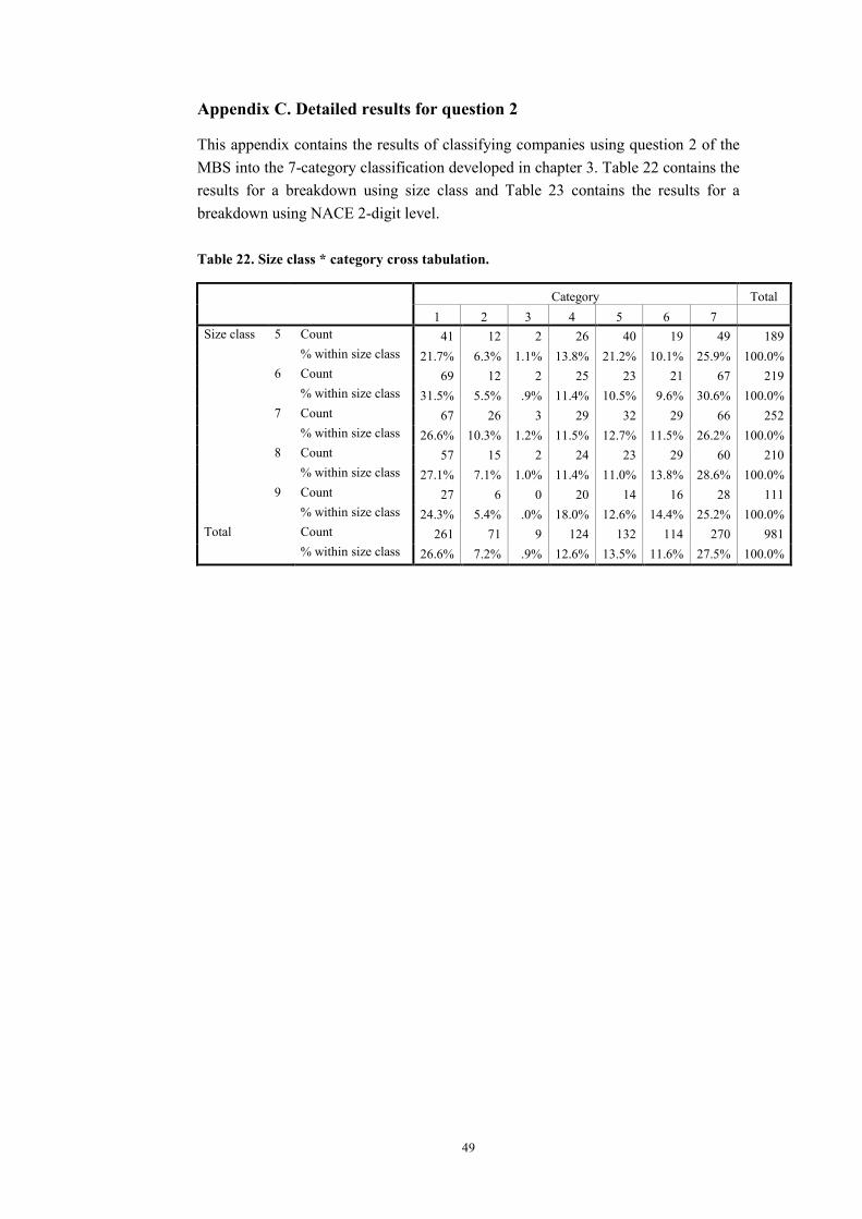
49

Appendix C. Detailed results for question 2

This appendix contains the results of classifying companies using question 2 of the MBS into the 7-category classification developed in chapter 3. Table 22 contains the results for a breakdown using size class and Table 23 contains the results for a breakdown using NACE 2-digit level.

Table 22. Size class * category cross tabulation.

Category Total 1 2 3 4 5 6 7

Size class 5 Count 41 12 2 26 40 19 49 189% within size class 21.7% 6.3% 1.1% 13.8% 21.2% 10.1% 25.9% 100.0%

6 Count 69 12 2 25 23 21 67 219% within size class 31.5% 5.5% .9% 11.4% 10.5% 9.6% 30.6% 100.0%

7 Count 67 26 3 29 32 29 66 252% within size class 26.6% 10.3% 1.2% 11.5% 12.7% 11.5% 26.2% 100.0%

8 Count 57 15 2 24 23 29 60 210% within size class 27.1% 7.1% 1.0% 11.4% 11.0% 13.8% 28.6% 100.0%

9 Count 27 6 0 20 14 16 28 111% within size class 24.3% 5.4% .0% 18.0% 12.6% 14.4% 25.2% 100.0%

Total Count 261 71 9 124 132 114 270 981% within size class 26.6% 7.2% .9% 12.6% 13.5% 11.6% 27.5% 100.0%

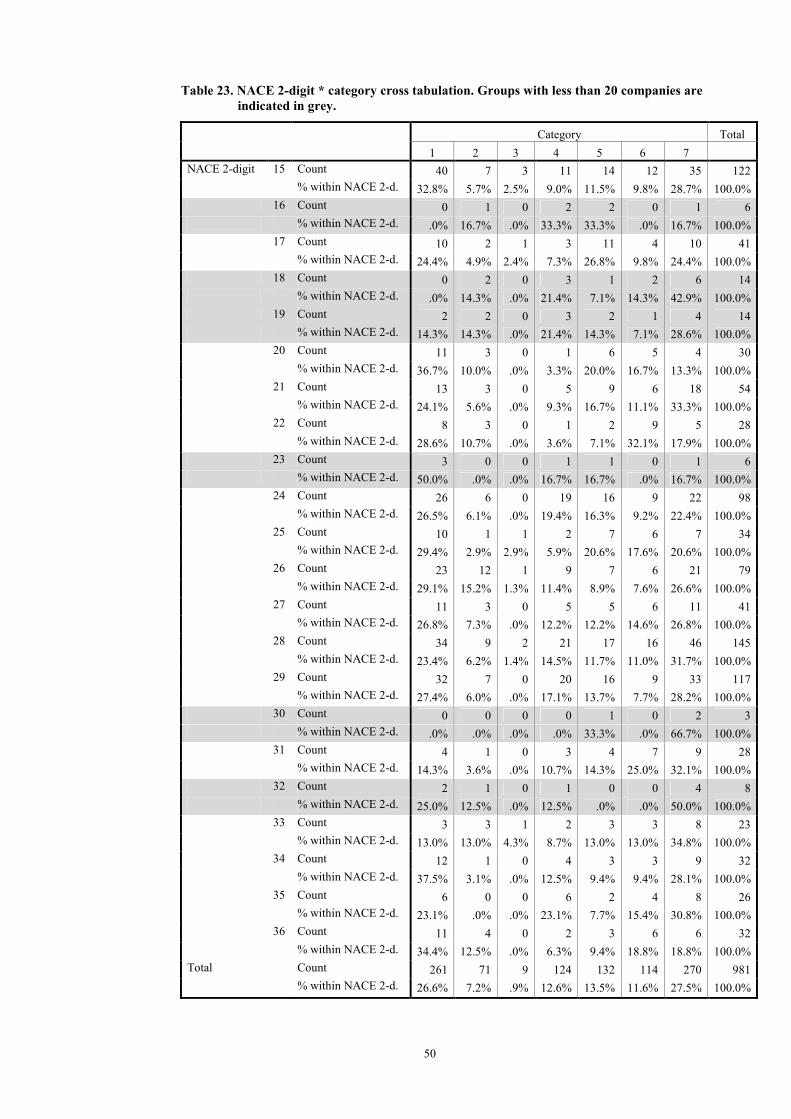
50

Table 23. NACE 2-digit * category cross tabulation. Groups with less than 20 companies are indicated in grey.

Category Total 1 2 3 4 5 6 7

NACE 2-digit 15 Count 40 7 3 11 14 12 35 122% within NACE 2-d. 32.8% 5.7% 2.5% 9.0% 11.5% 9.8% 28.7% 100.0%

16 Count 0 1 0 2 2 0 1 6% within NACE 2-d. .0% 16.7% .0% 33.3% 33.3% .0% 16.7% 100.0%

17 Count 10 2 1 3 11 4 10 41% within NACE 2-d. 24.4% 4.9% 2.4% 7.3% 26.8% 9.8% 24.4% 100.0%

18 Count 0 2 0 3 1 2 6 14% within NACE 2-d. .0% 14.3% .0% 21.4% 7.1% 14.3% 42.9% 100.0%

19 Count 2 2 0 3 2 1 4 14% within NACE 2-d. 14.3% 14.3% .0% 21.4% 14.3% 7.1% 28.6% 100.0%

20 Count 11 3 0 1 6 5 4 30% within NACE 2-d. 36.7% 10.0% .0% 3.3% 20.0% 16.7% 13.3% 100.0%

21 Count 13 3 0 5 9 6 18 54% within NACE 2-d. 24.1% 5.6% .0% 9.3% 16.7% 11.1% 33.3% 100.0%

22 Count 8 3 0 1 2 9 5 28% within NACE 2-d. 28.6% 10.7% .0% 3.6% 7.1% 32.1% 17.9% 100.0%

23 Count 3 0 0 1 1 0 1 6% within NACE 2-d. 50.0% .0% .0% 16.7% 16.7% .0% 16.7% 100.0%

24 Count 26 6 0 19 16 9 22 98% within NACE 2-d. 26.5% 6.1% .0% 19.4% 16.3% 9.2% 22.4% 100.0%

25 Count 10 1 1 2 7 6 7 34% within NACE 2-d. 29.4% 2.9% 2.9% 5.9% 20.6% 17.6% 20.6% 100.0%

26 Count 23 12 1 9 7 6 21 79% within NACE 2-d. 29.1% 15.2% 1.3% 11.4% 8.9% 7.6% 26.6% 100.0%

27 Count 11 3 0 5 5 6 11 41% within NACE 2-d. 26.8% 7.3% .0% 12.2% 12.2% 14.6% 26.8% 100.0%

28 Count 34 9 2 21 17 16 46 145% within NACE 2-d. 23.4% 6.2% 1.4% 14.5% 11.7% 11.0% 31.7% 100.0%

29 Count 32 7 0 20 16 9 33 117% within NACE 2-d. 27.4% 6.0% .0% 17.1% 13.7% 7.7% 28.2% 100.0%

30 Count 0 0 0 0 1 0 2 3% within NACE 2-d. .0% .0% .0% .0% 33.3% .0% 66.7% 100.0%

31 Count 4 1 0 3 4 7 9 28% within NACE 2-d. 14.3% 3.6% .0% 10.7% 14.3% 25.0% 32.1% 100.0%

32 Count 2 1 0 1 0 0 4 8% within NACE 2-d. 25.0% 12.5% .0% 12.5% .0% .0% 50.0% 100.0%

33 Count 3 3 1 2 3 3 8 23% within NACE 2-d. 13.0% 13.0% 4.3% 8.7% 13.0% 13.0% 34.8% 100.0%

34 Count 12 1 0 4 3 3 9 32% within NACE 2-d. 37.5% 3.1% .0% 12.5% 9.4% 9.4% 28.1% 100.0%

35 Count 6 0 0 6 2 4 8 26% within NACE 2-d. 23.1% .0% .0% 23.1% 7.7% 15.4% 30.8% 100.0%

36 Count 11 4 0 2 3 6 6 32% within NACE 2-d. 34.4% 12.5% .0% 6.3% 9.4% 18.8% 18.8% 100.0%

Total Count 261 71 9 124 132 114 270 981% within NACE 2-d. 26.6% 7.2% .9% 12.6% 13.5% 11.6% 27.5% 100.0%

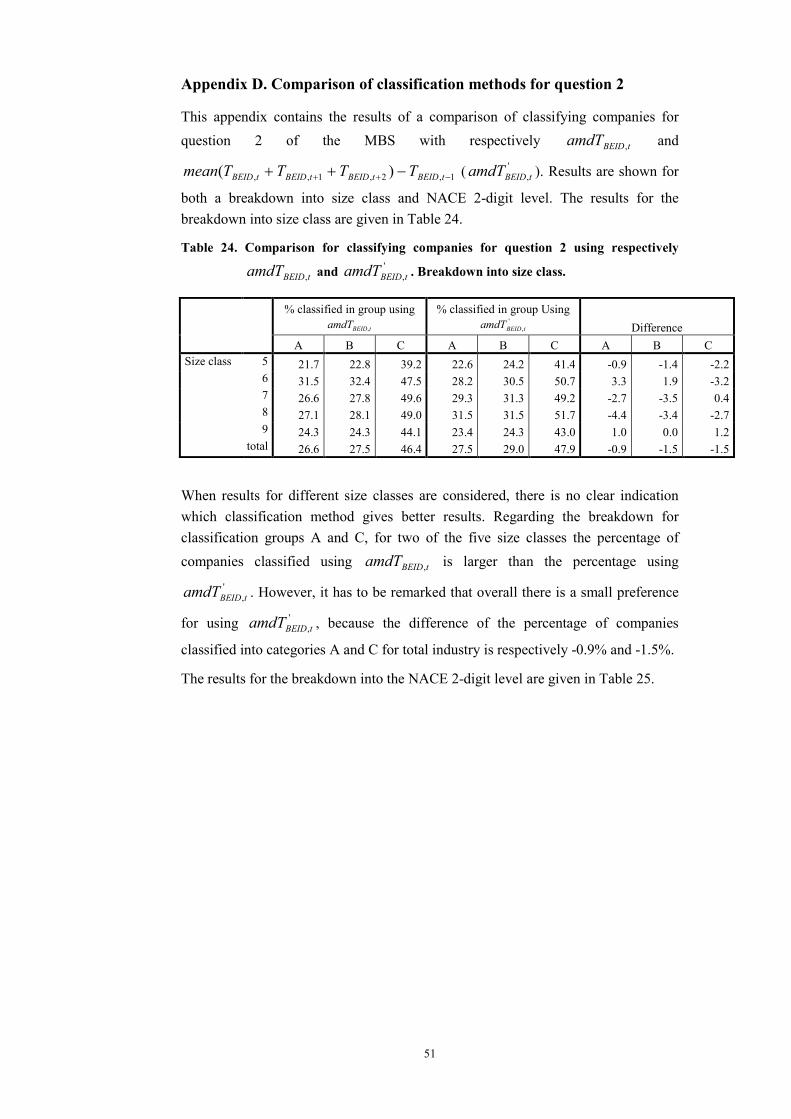
51

Appendix D. Comparison of classification methods for question 2

This appendix contains the results of a comparison of classifying companies for question 2 of the MBS with respectively tBEIDamdT , and

1,2,1,, )( −++ −++ tBEIDtBEIDtBEIDtBEID TTTTmean ( ',tBEIDamdT ). Results are shown for

both a breakdown into size class and NACE 2-digit level. The results for the breakdown into size class are given in Table 24.

Table 24. Comparison for classifying companies for question 2 using respectively

tBEIDamdT , and ',tBEIDamdT . Breakdown into size class.

% classified in group using % classified in group Using tBEIDamdT ,

',tBEIDamdT Difference

A B C A B C A B CSize class 5 21.7 22.8 39.2 22.6 24.2 41.4 -0.9 -1.4 -2.2

6 31.5 32.4 47.5 28.2 30.5 50.7 3.3 1.9 -3.27 26.6 27.8 49.6 29.3 31.3 49.2 -2.7 -3.5 0.48 27.1 28.1 49.0 31.5 31.5 51.7 -4.4 -3.4 -2.79 24.3 24.3 44.1 23.4 24.3 43.0 1.0 0.0 1.2

total 26.6 27.5 46.4 27.5 29.0 47.9 -0.9 -1.5 -1.5

When results for different size classes are considered, there is no clear indication which classification method gives better results. Regarding the breakdown for classification groups A and C, for two of the five size classes the percentage of companies classified using tBEIDamdT , is larger than the percentage using

',tBEIDamdT . However, it has to be remarked that overall there is a small preference

for using ',tBEIDamdT , because the difference of the percentage of companies

classified into categories A and C for total industry is respectively -0.9% and -1.5%.

The results for the breakdown into the NACE 2-digit level are given in Table 25.

52

Table 25. Comparison for classifying companies for question 2 using respectively

tBEIDamdT , and ',tBEIDamdT . Breakdown into NACE 2-digit level.

% classified in group using % classified in group using tBEIDamdT ,

',tBEIDamdT Difference

A B C A B C A B CNACE 2-digit 15 32.8 35.2 50.8 30.8 32.5 52.5 2.0 2.7 -1.7

16 0.0 0.0 16.7 16.7 16.7 16.7 -16.7 -16.7 0.017 24.4 26.8 41.5 17.5 20.0 40.0 6.9 6.8 1.518 0.0 0.0 28.6 0.0 7.7 30.8 0.0 -7.7 -2.219 14.3 14.3 35.7 15.4 23.1 30.8 -1.1 -8.8 4.920 36.7 36.7 63.3 34.5 37.9 69.0 2.2 -1.3 -5.621 24.1 24.1 40.7 21.2 21.2 42.3 2.9 2.9 -1.622 28.6 28.6 71.4 46.4 46.4 75.0 -17.9 -17.9 -3.623 50.0 50.0 50.0 50.0 50.0 50.0 0.0 0.0 0.024 26.5 26.5 41.8 25.0 26.0 43.8 1.5 0.5 -1.925 29.4 32.4 52.9 41.2 41.2 58.8 -11.8 -8.8 -5.926 29.1 30.4 53.2 34.6 34.6 57.7 -5.5 -4.2 -4.527 26.8 26.8 48.8 30.0 35.0 55.0 -3.2 -8.2 -6.228 23.4 24.8 42.1 26.4 27.1 43.1 -2.9 -2.3 -1.029 27.4 27.4 41.0 24.6 24.6 40.4 2.8 2.8 0.730 0.0 0.0 0.0 0.0 0.0 0.0 0.0 0.0 0.031 14.3 14.3 42.9 16.0 16.0 32.0 -1.7 -1.7 10.932 25.0 25.0 37.5 28.6 28.6 57.1 -3.6 -3.6 -19.633 13.0 17.4 43.5 33.3 38.1 52.4 -20.3 -20.7 -8.934 37.5 37.5 50.0 32.3 35.5 54.8 5.2 2.0 -4.835 23.1 23.1 38.5 11.1 11.1 25.9 12.0 12.0 12.536 34.4 34.4 65.6 35.7 42.9 67.9 -1.3 -8.5 -2.2total 26.6 27.5 46.4 27.5 29.0 47.9 -0.9 -1.5 -1.5

For 8 of the 16 analysed NACE 2-digit levels the percentage of companies classified into group A is larger using tBEIDamdT , , indicating that there is no clear sign which

classification method gives better results. When group C is analysed, for only 4 of the 16 NACE 2-digit levels the percentage of companies classified using

tBEIDamdT , is larger. This indicates a preference for classifying companies using '

,tBEIDamdT .

Overall, there seems to be a small preference to use ',tBEIDamdT for classifying

companies for question 2 of the MBS. However, the results presented in this appendix indicate, that there are size classes and NACE 2-digit groups for which using tBEIDamdT , gives better results. To determine how the results of question 2

exactly have to be interpreted in practice remains a topic for future research.

53

Appendix E. X12-ARIMA Setups

1: SERIES{ 2: title = "AOFM" 3: Format = "DateValue" 4: Period = 12 5: File = "d:\temp\vivaldi\10000232.DAT" 6: name = "100002" 7: precision = 0 8: decimals = 0 9: } 10: TRANSFORM{ 11: Function = auto 12: adjust = none 13: savelog=atr 14: } 15: AUTOMDL{ 16: file = "\\mspv1f\Programma1\ImplSTS\Seizoen\VivX12\VIVW2K\x12\x12a.mdl" 17: mode = fcst 18: method = best 19: Identify = first 20: }

54

1: SERIES{ 2: title = "NTLY" 3: Format = "DateValue" 4: Period = 12 5: File = "d:\temp\vivaldi\10000232.DAT" 6: name = "100002" 7: precision = 0 8: decimals = 0 9: } 10: TRANSFORM{ 11: Function = none 12: adjust = none 13: savelog=atr 14: } 15: REGRESSION{ 16: Variables =( 17: lpyear 18: ) 19: save = (ao ls td ) 20: 21: } 22: AUTOMDL{ 23: file = "\\mspv1f\Programma1\ImplSTS\Seizoen\VivX12\VIVW2K\x12\x12a.mdl" 24: mode = fcst 25: method = best 26: Identify = first 27: } 28: ESTIMATE{ 29: maxiter = 999 30: } 31: FORECAST{ 32: Maxlead = 0 33: }

55

1: SERIES{ 2: title = "LTLY" 3: Format = "DateValue" 4: Period = 12 5: File = "d:\temp\vivaldi\10002545.DAT" 6: name = "100025" 7: precision = 0 8: decimals = 0 9: } 10: TRANSFORM{ 11: Function = log 12: adjust = none 13: savelog=atr 14: } 15: REGRESSION{ 16: Variables =( 17: lpyear 18: ) 19: save = (ao ls td) 20: } 21: AUTOMDL{ 22: file = "\\mspv1f\Programma1\ImplSTS\Seizoen\VivX12\VIVW2K\x12\x12a.mdl" 23: mode = fcst 24: method = best 25: Identify = first 26: } 27: ESTIMATE{ 28: maxiter = 999 29: } 30: FORECAST{ 31: Maxlead = 0 32: }

56

1: SERIES{ 2: title = "NTWW" 3: Format = "DateValue" 4: Period = 12 5: File = "d:\temp\vivaldi\10000232.DAT" 6: name = "100002" 7: precision = 0 8: decimals = 0 9: } 10: TRANSFORM{ 11: Function = none 12: adjust = none 13: savelog=atr 14: } 15: REGRESSION{ 16: Variables =( 17: td1nolpyear 18: ) 19: save = (ao ls td ) 20: 21: } 22: AUTOMDL{ 23: file = "\\mspv1f\Programma1\ImplSTS\Seizoen\VivX12\VIVW2K\x12\x12a.mdl" 24: mode = fcst 25: method = best 26: Identify = first 27: } 28: ESTIMATE{ 29: maxiter = 999 30: } 31: FORECAST{ 32: Maxlead = 0 33: } 34: X11{ 35: mode = add 36: seasonalma = msr 37: sigmalim = (1.20 2.00) 38: save=(b1 d8 d10 d11 seasonal) 39: final = (ao ls) 40: appendfcst=yes 41: savelog = (m2 m7 m10 m11 q q2) 42: }

57

1: SERIES{ 2: title = "LTWW" 3: Format = "DateValue" 4: Period = 12 5: File = "d:\temp\vivaldi\10002545.DAT" 6: name = "100025" 7: precision = 0 8: decimals = 0 9: } 10: TRANSFORM{ 11: Function = log 12: adjust = none 13: savelog=atr 14: } 15: REGRESSION{ 16: Variables =( 17: td1nolpyear 18: ) 19: save = (ao ls td) 20: } 21: AUTOMDL{ 22: file = "\\mspv1f\Programma1\ImplSTS\Seizoen\VivX12\VIVW2K\x12\x12a.mdl" 23: mode = fcst 24: method = best 25: Identify = first 26: } 27: ESTIMATE{ 28: maxiter = 999 29: } 30: FORECAST{ 31: Maxlead = 0 32: } 33: X11{ 34: mode = mult 35: seasonalma = msr 36: sigmalim = (1.20 2.00) 37: save=(b1 d8 d10 d11 seasonal) 38: final = (ao ls) 39: appendfcst=yes 40: savelog = (m2 m7 m10 m11 q q2) 41: }

58

1: SERIES{ 2: title = "NT6D" 3: Format = "DateValue" 4: Period = 12 5: File = "d:\temp\vivaldi\10000232.DAT" 6: name = "100002" 7: precision = 0 8: decimals = 0 9: } 10: TRANSFORM{ 11: Function = none 12: adjust = none 13: savelog=atr 14: } 15: REGRESSION{ 16: Variables =( 17: tdnolpyear 18: ) 19: save = (ao ls td ) 20: 21: } 22: AUTOMDL{ 23: file = "\\mspv1f\Programma1\ImplSTS\Seizoen\VivX12\VIVW2K\x12\x12a.mdl" 24: mode = fcst 25: method = best 26: Identify = first 27: } 28: ESTIMATE{ 29: maxiter = 999 30: } 31: FORECAST{ 32: Maxlead = 0 33: } 34: X11{ 35: mode = add 36: seasonalma = msr 37: sigmalim = (1.20 2.00) 38: save=(b1 d8 d10 d11 seasonal) 39: final = (ao ls) 40: appendfcst=yes 41: savelog = (m2 m7 m10 m11 q q2) 42: }

59

1: SERIES{ 2: title = "LT6D" 3: Format = "DateValue" 4: Period = 12 5: File = "d:\temp\vivaldi\10002545.DAT" 6: name = "100025" 7: precision = 0 8: decimals = 0 9: } 10: TRANSFORM{ 11: Function = log 12: adjust = none 13: savelog=atr 14: } 15: REGRESSION{ 16: Variables =( 17: tdnolpyear 18: ) 19: save = (ao ls td) 20: } 21: AUTOMDL{ 22: file = "\\mspv1f\Programma1\ImplSTS\Seizoen\VivX12\VIVW2K\x12\x12a.mdl" 23: mode = fcst 24: method = best 25: Identify = first 26: } 27: ESTIMATE{ 28: maxiter = 999 29: } 30: FORECAST{ 31: Maxlead = 0 32: } 33: X11{ 34: mode = mult 35: seasonalma = msr 36: sigmalim = (1.20 2.00) 37: save=(b1 d8 d10 d11 seasonal) 38: final = (ao ls) 39: appendfcst=yes 40: savelog = (m2 m7 m10 m11 q q2) 41: }

60

1: SERIES{ 2: title = "NTNOWD" 3: Format = "DateValue" 4: Period = 12 5: File = "d:\temp\vivaldi\10000232.DAT" 6: name = "100002" 7: precision = 0 8: decimals = 0 9: } 10: TRANSFORM{ 11: Function = none 12: adjust = none 13: savelog=atr 14: } 15: AUTOMDL{ 16: file = "\\mspv1f\Programma1\ImplSTS\Seizoen\VivX12\VIVW2K\x12\x12a.mdl" 17: mode = fcst 18: method = best 19: Identify = first 20: } 21: ESTIMATE{ 22: maxiter = 999 23: } 24: FORECAST{ 25: Maxlead = 0 26: } 27: X11{ 28: mode = add 29: seasonalma = msr 30: sigmalim = (1.20 2.00) 31: save=(b1 d8 d10 d11 seasonal) 32: final = (ao ls) 33: appendfcst=yes 34: savelog = (m2 m7 m10 m11 q q2) 35: }

61

1: SERIES{ 2: title = "LTNOWD" 3: Format = "DateValue" 4: Period = 12 5: File = "d:\temp\vivaldi\10002545.DAT" 6: name = "100025" 7: precision = 0 8: decimals = 0 9: } 10: TRANSFORM{ 11: Function = log 12: adjust = none 13: savelog=atr 14: } 15: AUTOMDL{ 16: file = "\\mspv1f\Programma1\ImplSTS\Seizoen\VivX12\VIVW2K\x12\x12a.mdl" 17: mode = fcst 18: method = best 19: Identify = first 20: } 21: ESTIMATE{ 22: maxiter = 999 23: } 24: FORECAST{ 25: Maxlead = 0 26: } 27: X11{ 28: mode = mult 29: seasonalma = msr 30: sigmalim = (1.20 2.00) 31: save=(b1 d8 d10 d11 seasonal) 32: final = (ao ls) 33: appendfcst=yes 34: savelog = (m2 m7 m10 m11 q q2) 35: }

62

Appendix F. NACE Classification

This appendix gives in Table 26 the description of the different NACE 2-digit categories used in this paper.

Table 26. Description of NACE 2-digit level.

NACE Manufacture of15 Food products and beverages16 Tobacco products17 Textiles18 Wearing apparel19 Leather (and products)20 Wood (and products)21 Paper, paperboard (and products)22 Publishing, printing and reproduction23 Coke, refined petroleum and nuclear fuel24 Chemicals (and products)25 Rubber and plastic products26 Glass, earthenware, cement, lime and plaster articles27 Basic metals28 Fabricated metal products29 Machinery and equipment30 Office machinery and computers31 Other electrical machinery and apparatus32 Radio, television and communication equipment and apparatus33 Medical, precision and optical instruments, watches and clocks34 Motor vehicles, trailers and semi-trailers35 Other transport equipment36 Furniture and other manufacturing n.e.c.