A constrained binary knapsack approximation for shortest path network interdiction

Computers & Industrial Engineering 61 (2011) 981–992

Contents lists available at ScienceDirect

Computers & Industrial Engineering

journal homepage: www.elsevier .com/ locate/caie

A constrained binary knapsack approximation for shortest path network interdiction

Justin Yates ⇑, Kavitha LakshmananDepartment of Industrial and Systems Engineering, Texas A&M University, United States

a r t i c l e i n f o a b s t r a c t

Article history:Received 6 December 2010Received in revised form 11 May 2011Accepted 14 June 2011Available online 17 June 2011

Keywords:Network interdictionHomeland securityApproximation techniquesInteger programming

0360-8352/$ - see front matter � 2011 Elsevier Ltd. Adoi:10.1016/j.cie.2011.06.011

⇑ Corresponding author. Address: Department of Ineering, Texas A&M University, 237D Zachry EnginCollege Station, TX 77843-3131, United States. Tel.: +

E-mail addresses: [email protected] (J. Yates),(K. Lakshmanan).

A modified shortest path network interdiction model is approximated in this work by a constrained bin-ary knapsack which uses aggregated arc maximum flow as the objective function coefficient. In the mod-ified shortest path network interdiction problem, an attacker selects a path of highest non-detectionprobability on a network with multiple origins and multiple available targets. A defender allocates a lim-ited number of resources within the geographic region of the network to reduce the maximum networknon-detection probability between all origin-target pairs by reducing arc non-detection probabilities andwhere path non-detection probability is modeled as a product of all arc non-detection probabilities onthat path. Traditional decomposition methods to solve the shortest path network interdiction problemare sensitive to problem size and network/regional complexity. The goal of this paper is to develop amethod for approximating the regional allocation of defense resources that maintains accuracy whilereducing both computational effort and the sensitivity of computation time to network/regional proper-ties. Statistical and spatial analysis methods are utilized to verify approximation performance of theknapsack method in two real-world networks.

� 2011 Elsevier Ltd. All rights reserved.

1. Introduction

Shortest path network interdiction may be considered as eithera deterministic or stochastic attacker-defender game played withlimited resources over a connected network with sequential move-ment. These games may be played with perfect, imperfect, orasymmetric knowledge, discrete or continuous interdiction, andhave been applied to a wide array of applications in homelandsecurity and defense which include but are not limited to portsecurity, border patrol, and the protection of critical infrastructure.As focus on these interdiction problems has increased in recentyears, so too has the desire to model more complex networksand interdiction scenarios. Such increases in complexity and scopehave necessitated the examination of alternative solution andapproximation approaches to the traditional shortest path networkinterdiction problem due to the inability of optimal solution tech-niques to maintain computational tractability with the addedscope.

In order to effectively demonstrate the viability of alternatesolution approaches to the shortest path network interdictionproblem, it is necessary to examine not only the capability to

ll rights reserved.

ndustrial and Systems Engi-eering Center, 3131 TAMU,1 979 845 [email protected]

approximate the computational solution but the spatial solutionas well. The desire to closely approximate computational resultsis relatively obvious. Reliable solution techniques need to illustrateconsistency in their ability to return optimal values and solutionsthat provide accurate numerical approximations. As an example,the probability of damage to critical infrastructure, the probabilityto detect a covert adversary, or the probability to identify illicitmaterials inside of a container, are all examples of computationalmetrics which would be used to evaluate the appropriateness ofany proposed resource allocations or policy procedures. The desireto closely approximate spatial results, however, is arguably just asvital to the success and confidence of approximation procedures.When employing approximation models, there exists the real po-tential for multiple redundant solutions (naturally, this dependson the modelers’ choices in formulation, network representation,network parameter assignment, etc.) which could yield the sameoptimal value through significantly different spatial resource allo-cations. Allocating resources to sub-optimal locations could lead todisastrous results including the loss of life and infrastructure, aswell as large fiscal and psychological burdens for the attackedregion and its population. It is imperative, therefore, that anydeveloped approximate procedures for such scenarios be ade-quately vetted and tested to ensure their reliability and capabilityto produce results that are both computationally and spatially true.

Recognition of the need for competent approximation proce-dures in network interdiction has been directly stated (Church &Scaparra, 2007; Lim & Smith, 2007). Algorithmic/heuristic

http://dx.doi.org/10.1016/j.cie.2011.06.011

mailto:[email protected]

mailto:[email protected]

http://dx.doi.org/10.1016/j.cie.2011.06.011

http://www.sciencedirect.com/science/journal/03608352

http://www.elsevier.com/locate/caie

Nomenclature

A set of suitable sensor locationsK set of network arcsa weight of objective criterion where 0 6 a 6 1B total allowable defense budgetcs cost to locate sensor type s 2 Skni binary variable where kni = 1 if arc i 2K is incident to

node n 2 N, otherwise kni = 0mj aggregate maximum flow over arc j 2KN set of network nodesgs sensitivity of sensor s with 0 6 gs 6 1pj number of network intersections separating arc j 2K

from its closest network originqn {1,�1,0} if node n is an {origin, destination, intermedi-

ate}ub objective function coefficient for atom b 2 ARas set of arcs falling within the range of influence of a type

s sensor located at atom a 2 Aras

i binary variable representing whether an arc is capableof being covered ras

i ¼ 1� �

by a type s sensor located atatom a or not ras

i ¼ 0� �

S set of sensor types available for location

/j set of atoms covering arc j 2Ks maximum allowable sensor coverageuist non-detection probability for arc i 2K under the cover-

age of t type s sensors

Decision variableswi wi = 1 if arc i 2K used in the attacker path, otherwise

wi = 0yas yas = 1 if sensor type s 2 S located at a 2 A, otherwise

yas = 0xist xis = 1 if i 2K covered by t type s 2 S sensors, otherwise

xist = 0vb vb = 1 if atom b 2 A is used, otherwise vb = 0

AcronymsBD benders decompositionCIKR critical infrastructure and key resourcesKNAP constrained knapsack approximationGIS geographic information systemDSPNI discrete shortest path network interdiction problem

982 J. Yates, K. Lakshmanan / Computers & Industrial Engineering 61 (2011) 981–992

combinations as well as heuristic methods have been employed toobtain solutions to deterministic and stochastic network interdic-tion problems (Held & Woodruff, 2005; Royset & Wood, 2007;Salmeron, Wood, &Baldick,Bald). Within the current literature(including those papers cited above), focus on algorithmic/heuris-tic performance relies almost exclusively on a computationalbarometer. Often formulated as bi-level or multi-objective prob-lems, the developed network interdiction approximation proce-dures work well to combat the computational time burdenobserved in obtaining an optimal solution. Even for small net-works, the computational effort required to solve these problemscan be significant.

A common approach in the literature to solve the networkinterdiction problems is to implement some form of BendersDecomposition, effectively sub-dividing the larger multi-objectiveproblem into a master problem and sub problem which can thenbe solved iteratively to obtain an optimal solution. This approachcan be observed in (Brown, Carlyle, Salmeron, & Wood, 2006;Israeli & Wood, 2002; Yates & Casas, 2010). In practice, the masterproblem tends to scale poorly with relation to increases in networksize and complexity and, overall, tends to require the majority ofcomputational effort (as an example, Brown et al., 2006, indicateup to 90% of computation time in obtaining an optimal interdictionsolution was spent solving the master problem). Approximationprocedures may attempt to reduce the number of Benders Decom-position iterations (and thus the number of times the master prob-lem needs to be solved) through cut generation or the addition ofother inequality constraints. For problems of the size typically con-sidered in the literature, such approaches may be viable (e.g., 200arcs, 50 nodes). For truly large-scale, regionally representative net-works, however (e.g. 200,000 + arcs, 10,000 + nodes), even one iter-ation of the master problem may be computationally prohibitive. Itis for this reason that reliable approximate procedures and meth-ods which are not hindered by such combinatorial properties aresought and desired within the network interdiction domain.

This paper examines the discrete shortest path networkinterdiction problem (DSPNI) with perfect information in a two-player attacker-defender game and develops a knapsack-basedsolution approach for obtaining strong computational and spatial

approximations to the optimal DSPNI solution. The motivationfor this approach lies in the desire to accurately and consistentlyapproximate both the optimal objective value and the spatial loca-tion of allocated resources in a single, simplistic model that doesnot suffer computationally from the same problems of scale ob-served in Benders Decomposition and other algorithmic/heuristicapproaches. The DSPNI model used as a base-line in this paperwas first introduced in (Yates & Casas, 2010) and modifies the tra-ditional DSPNI by augmenting the spatial emphasis placed on re-source allocation. The remainder of this paper is organized in thefollowing way. Section 2 supports development of and presents aformulation for the knapsack approximation model, introduces ter-minology which will be used throughout the paper, and discussesthe DSPNI problem examined. Section 3 introduces two test-casenetworks from Los Angeles County, California that will be exam-ined within a structured experimental design to assess the compu-tational and spatial performance of the proposed knapsackapproximation. Sections 4 and 5 analyze the results of the experi-mental design computationally and spatially, respectively. Section6 concludes this paper.

2. Approach and approximation

The goal of this paper is to develop a knapsack-based methodfor approximating computational and spatial solutions to theDSPNI. Motivating this work is the observation that currentprocedures for obtaining optimal solutions to DSPNI become com-putationally prohibitive as network size/complexity increases,inhibiting the ability of policy and decision makers to obtain solu-tions in a timely manner (or in the case of large-scale networks,obtain any solution at all). When interpreting the DSPNI in termsof public policy decisions, the primary objective is to effectivelylocate defense resources within the given region. Determiningthese resource locations is thus the primary concern and directoutput of the developed approximation.

To develop a reliable approximation, the authors examineincorporation of maximum-flow/min-cut into a multi-objective,constrained knapsack formulation. This section introduces

J. Yates, K. Lakshmanan / Computers & Industrial Engineering 61 (2011) 981–992 983

necessary terminology for discussion of the developed knapsackmodel as well as the DSPNI formulation utilized as the optimalbaseline within the experimental design.

2.1. Discrete shortest path network interdiction

The DSPNI problem in this paper consists of a perfect informa-tion attacker-defender game modeled as a critical infrastructureprotection scenario. The attacker and defender move sequentiallywith perfect knowledge of their adversary’s respective decision ateach iteration. A connected, bi-directional network G(N,K) and aset of acceptable defense sensor locations A (these potential sensorlocations are referred to through the remainder of the paper asatoms) structure the regional setting for the problem. The problemis solved to optimality using BD to iteratively solve a set of sub-problems into which the original formulation may be divided(Bard, 1998). At each iteration of the Benders implementation,the attacker considers the current defender sensor resource alloca-tion and selects a complete path of maximum non-detection prob-ability from a pre-defined set of origins to a pre-defined set ofcritical infrastructure (origins and critical infrastructure networknodes are disjoint subsets of the network node set N). The defenderthen considers the newly obtained attacker path. If this path has al-ready been considered by the defender, then iterations terminatewith a provably optimal solution (Bard, 1998). If this path hasnot yet been considered, then it is introduced into the defendersub-problem as a new constraint and a new sensor resource alloca-tion which minimizes the maximum path non-detection probabil-ity for the network is determined. As the DSPNI problem is not themajor focus of this paper, the inquisitive reader is directed to(Yates & Casas, 2010) for a more detailed discussion of this formu-lation and its solution approach. A brief overview of the formula-tion follows.

The DSPNI has one attacker variable and two defender variables.The defender requires two decision variables due to the allocationof resources at atoms instead of directly on network arcs. One deci-sion variable determines where sensor resources are located whilethe second decision variable relates this sensor resource coverageto its actual influence/impact on the arcs of the network. TheDSPNI formulation is now provided.

[DSPNI]

z ¼min maxQi;s;t

uwixistist

s:t:P

ikniwi 6 qn 8n

xist � 1t

Pa

rasi yas 6 0 8i; s; tP

s;txist ¼ 1 8iP

a;scsyas 6 B

w; x; y 2 f0;1g

The overall objective z of DSPNI is to minimize the maximum pathnon-detection probability for the entire network. Constraint 1 en-sures that the attacker always selects a complete path throughthe network. Constraint 2 restricts arc influence to be at most thenumber of located sensors the arc is covered by. Constraint 3 en-sures arc coverage and is necessary to accurately assess z while con-straint 4 restricts sensor resource allocation to a budget.

The DSPNI and BD approach work well for small networkswhich can be easily solved using standard commercial optimiza-tion solvers such as CPLEX. As network size increases, however,problem size begins to prohibit the modelers’ ability to obtainquick solutions through this approach. In practice, the attackerpath identification Benders sub-problem will solve easily resulting

in nearly all of the computational expense for the DSPNI problemto be expended solving the defender sub-problem (Brown et al.,2006). Even as network size reaches moderate levels (e.g. 1500 di-rected arcs, 400 nodes), total computation time can easily extendinto multiple hours. This observed rapid acceleration in computa-tion time and the need for policy and decision makers to capablyand confidently run many alternate scenarios in time-sensitive sit-uations ultimately motivates this work.

2.2. Knapsack approximation

The developed approximation technique integrates maximumflow within a constrained binary knapsack optimization model.Exploiting max-flow/min-cut algorithms and solutions to obtainnetwork interdiction approximations is not new to the literature.Traditionally, approaches for modeling network interdiction havefocused on identifying arcs or nodes most critical to some interpre-tation of system performance. For instance, increasing the costassociated with routing flow between an origin–destination (O–D) pair is a common goal. Given the objective of increasing trans-portation costs, the impact of total or partial interdiction of arcs/nodes can be considered as either: (1) decreasing network capac-ity, preventing flow or forcing flow over more costly alternatepaths; or, (2) increasing the cost associated with minimal costpaths. Both aspects of interdiction rely on negatively affecting net-work connectivity in some way. A classic network analysis ap-proach to impacting connectivity between an O–D pair isthrough the identification of a cut set, or a set of arcs whose re-moval prevents O–D flow (Matisziw, Murray, & Grubesic, 2007).

Provided that interdiction efforts are limited by available re-sources, it is reasonable to focus on components of the smallestcut set possible (Wood, 2003). This basic idea was implementedas an integer program. It has been well established that solutionof the maximum-flow model corresponds to a minimum capacitycut; hence, it is no surprise that this relationship has beenexploited in the formulation of many interdiction models (Burchet al., 2003; Corley & Chang, 1974; Cunningham, 1985; Ghare,Montgomery, & Turner, 1971; Phillips, 1993; Ratliff, Sicilia, & Lu-bore, 1975; Wollmer, 1964; Wood, 2003). These references inte-grate/exploit maximum-flow properties within interdictionproblems in a myriad of ways. (Corley & Chang, 1974) deals withthe problem of identifying vital nodes by constructing an aug-mented network and reducing the problem to the identificationof vital arcs. (Burch et al., 2003) uses a linear relaxation for theinteger problem in polynomial time while (Wood, 2003) looks intoreformulation of linear relaxations to get tighter bounds. (Ghareet al., 1971) proposes a branch and bound algorithm and (Ratliffet al., 1975) sequentially modifies the network in an iterative ap-proach. (Phillips, 1993) describes three pseudo polynomial timealgorithms using maximum-flow properties for network interdic-tion and (Cunningham, 1985) illustrates an efficient greedy algo-rithm for this purpose. (Wollmer, 1964) performs sensitivityanalysis of networks and analyzes how removing certain arcs affectthe system.

Models based upon a maximum-flow model generally seek toapply limited interdiction resources to minimize the network’scapacity to move flow between origins and destinations. Toachieve this goal, minimal cut sets can be identified for an O–D pair(s). No other cut set can be contained within a minimal cut set. Aminimum capacity cut set then is a cut set of the smallest totalweight. The usefulness of the maximum flow-minimum cut theo-rem is that the total capacity of a minimum cut set correspondsto the maximum amount of flow capable of moving between anO–D on the network (Ford & Fulkerson, 1962). Once minimumcapacity cuts are found, arcs in these cuts can be assumed to belikely candidates for attack. The task then becomes determining


which component arcs would be interdicted under a budgetaryscenario. In this type of model, lower flow capacity remaining inthe network indicates a more effective interdiction plan.

Though a minimum cut set may indeed be effective for interdic-tion in certain circumstances, it has been suggested that solution tosome problems may require assessment of other minimal cut sets.For instance, if multiple interdiction objectives exist, a minimumcapacity cut for each O–D may not necessarily be the most effectiveoption (Balcioglu & Wood, 2003; Boyle, 1998). They use a partitionalgorithm to arrive at near optimal solutions taking into consider-ation secondary factors. Thus, the min cut approach can be used fornetwork interdiction problems as a heuristic approach as it yieldssolutions which are nearly optimal at a faster rate. Network Inter-diction problems are NP complete problems and hence min cutprovides a good start for approaching such problems.

Lemma. For any given network G(N,K) having probability of non-detection as its flow metric, the maximum flow in any path is an upperbound on the total path non-detection probability.

Proof. Let:

xi 2 [0,1] = the assigned non-detection probability value for alli 2K,q 2 Z+ = the numerical index assigned to a given path,P = the set of all arcs j 2K which comprise path q,lq = maximum flow for path q,sq = total non-detection probability for path q ¼

Qj2Pxj.

Assume that lq < sq for a random path q in the network G(N,K)comprised of arcs j 2 P and having assigned non-detection prob-abilities xj. For q, min(x1,x2, . . . ,xj) < (x1 � x2 � � � xj) by definition. Letx1 = min(x1,x2, . . . ,xj) be the maximum flow for q. If lq < sq, then(x2 � x3 � � � xj) > 1 necessitating that there exists at least one xj > 1 forj 2 {2,3, . . . , jPj} violating the initial condition xi 2 [0,1] for all i 2K.By contradiction, therefore, sq 6 lq.

Knapsack problems, like network interdiction problems, are NP-complete. Unlike network interdiction, however, the intensescrutiny given to knapsack problems in the literature has devel-oped a large body of knowledge regarding quick and accuratesolution procedures (Nemhauser and Wolsey, 1999). In addition,the knapsack formulation used to approximate DSPNI in this workis not effected by network size/scale/complexity to the extent thatDSPNI is. KNAP is now introduced and subsequently discussed. h

[KNAP]

z� ¼maxP

bubvb

s:t:P

bc1vb 6 BP

b2/j

vb 6 s 8j 2 K

v 2 f0;1g

ub ¼Xj2Rb1

amj þ1� a

pj

!

z� is the weighted objective utility for KNAP and contains two com-ponents. The first, mj, is the aggregated maximum flow for arc j con-sidering all origin and critical infrastructure pairs. The second, 1

pjis

the inverse of the node count between arc j and its closest origin.a determines the emphasis placed on the objective with the goalof KNAP to locate sensor resources at atoms of the network suchthat z� is maximized. In addition to the standard knapsack budget-ary constraint, KNAP also constrains the amount of tolerable sensoroverlap within a sensor allocation scheme in the same way thatDSPNI used the subscript index t to control the degree to which sen-sor overlap was counted when calculating z.

The resulting solution obtained by solving KNAP is a sensor allo-cation scheme within the network that satisfies a budget and dis-

courages excessive sensor overlap. The KNAP approximation doesnot provide information on attacker paths or network usage. It isnoted, however, that such information could be obtained withminimal effort by using the KNAP sensor allocation, network struc-ture and the origin and destination sets to solve a shortest pathproblem which returns the single best (or k best) attacker pathsunder the current sensor scheme. These paths would coincide withthose generated during implementation of the Bender’s techniqueto DSPNI (k Shortest path algorithms have been studied widely inthe literature and can be shown to operate in O (n log n) time wheren represents the number of network nodes).

3. Design and analysis

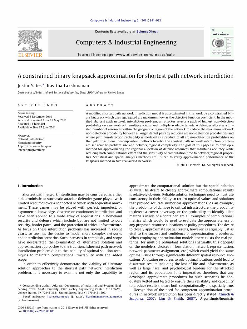
An experiment was designed to computationally and spatiallyevaluate performance of the knapsack approximation procedurewith the optimal DSPNI objective value obtained by implementingBD. The developed studies use two sub-networks of the Los Ange-les County, California road network and corresponding criticalinfrastructure. This data was obtained from the US Census Bureauand ArcGIS 9.3 was used to manage the data (US Census Bureau,2008). Fig. 1 displays the two sub-networks (Lancaster-Palmdaleand Northridge) and identifies set of origins and critical infrastruc-ture available to the attacker for each network (10 origins with 18critical infrastructure destinations for Lancaster-Palmdale and 10origins with 21 critical infrastructure destinations for Northridge).

In the experimental design, DSPNI was solved to optimality foreach combination of the following parameters:

� B: {$800,$1200,$1600,$2000}� ds: {0.2,0.4,0.6,0.8}, referred to as the sensor sensitivity� ui01: {Random, Uniform} where uist ¼ ui01

Qtds

KNAP was solved to optimality for each combination of the fol-lowing parameters:

� a: {0.0,0.01,0.02, . . . ,0.99,1.0}� B: {$200,$400, . . . , $3600,$3800}� s: {1,2,3,4}

The computational and spatial results obtained from the exper-imental design are discussed in the next two sections.

4. Computational analysis results and discussion

Computationally, the effectiveness of KNAP was determined byevaluating the optimal KNAP sensor scheme against the optimalDSPNI attacker path cuts. Recall that z is the optimal objectivevalue for DSPNI and call z0 the objective value obtained when thesensor scheme for the KNAP approximation is applied to the opti-mal attacker DSPNI attacker solution set. In this case, z acts as thetarget value with the difference between z and z0 indicating howwell KNAP approximates DSPNI computationally (the smaller theobserved difference, the closer z0 is to z numerically and thus thebetter the approximation). Computation time was also comparedbetween the alternate experimental runs for DSPNI and KNAP.

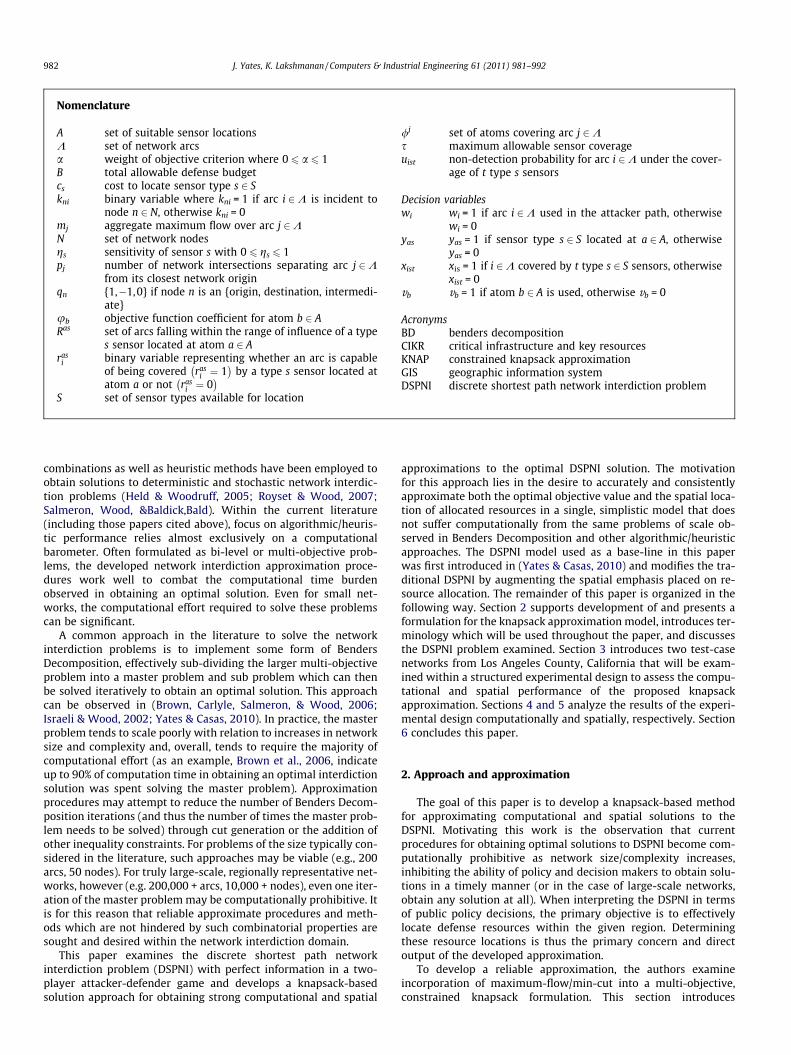
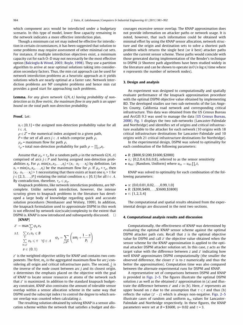
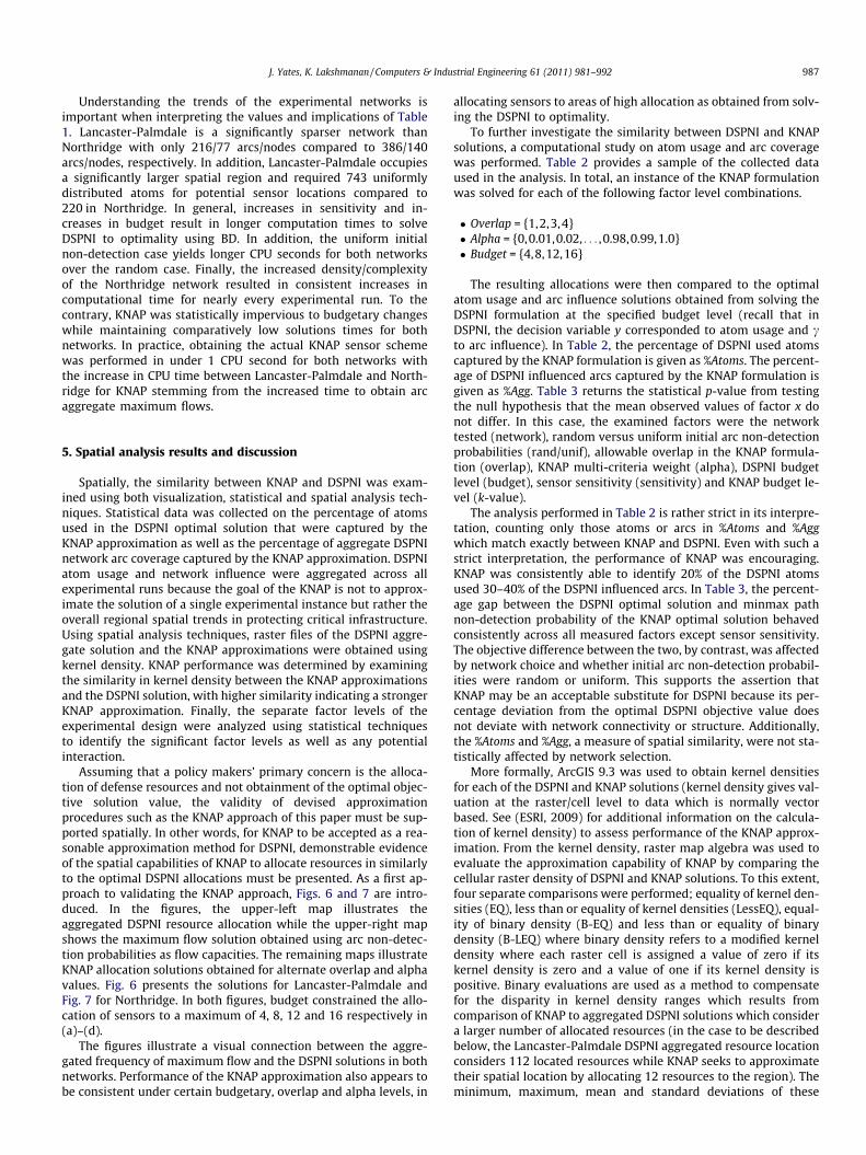
A representative set of comparisons between DSPNI and KNAPis provided in Figs. 2–5. The figures illustrate the optimal DSPNIsolution z as well as the obtained z0 approximation in (a) and illus-trate the difference between z0 and z in (b). Here, z0 represents anupper bound on z due to the assumption that s 6 t and thus (b)reflects the value (z0 - z) which is always non-negative. Figs. 2–5illustrate cases of random and uniform uist values for Lancaster-Palmdale and Northridge respectively. In these figures, the KNAPparameters were set at B = $3600, a= 0.02 and s = 3.

Fig. 1. Los Angeles County experimental sub-networks.

Fig. 2. Lancaster-Palmdale, random initial non-detection probability.

Fig. 3. Lancaster-Palmdale, uniform initial non-detection probability.


The figures clearly depict increased computational accuracy inapplying KNAP to the two cases of random arc non-detection andthe relatively poor capability for KNAP to approximate in the uni-form case. This is consistent with the properties expected in usingaggregate arc maximum flow as a surrogate for arc non-detectionprobability as discussed in Section 2. Maximum flow is more adeptat approximating in the random case due to the increased flowrestrictions of a heterogeneous network. The uniform case resultsin relatively homogenous aggregate arc maximum flows whichdo not contribute to a focused sensor allocation scheme. In bothLancaster-Palmdale and Northridge, the uniform cases resulted in

significantly higher observed differences and poorer consistencyin KNAP approximation for z. This trend actually serves tostrengthen support for KNAP as a DSPNI approximation in real-world applications as non-detection probability is often calculatedas a function of many various regional network and spatial proper-ties (e.g. network connectivity/density, line-of-sight, proximity tocritical infrastructure, slope, etc.). Considering the multiple crite-rion impacting arc non-detection probability, the derivative utilityvalue will almost certainly be heterogeneous across the network aseach of the contributing criterion will reflect certain degrees of het-erogeneity, the overall extent of which is captured in this work

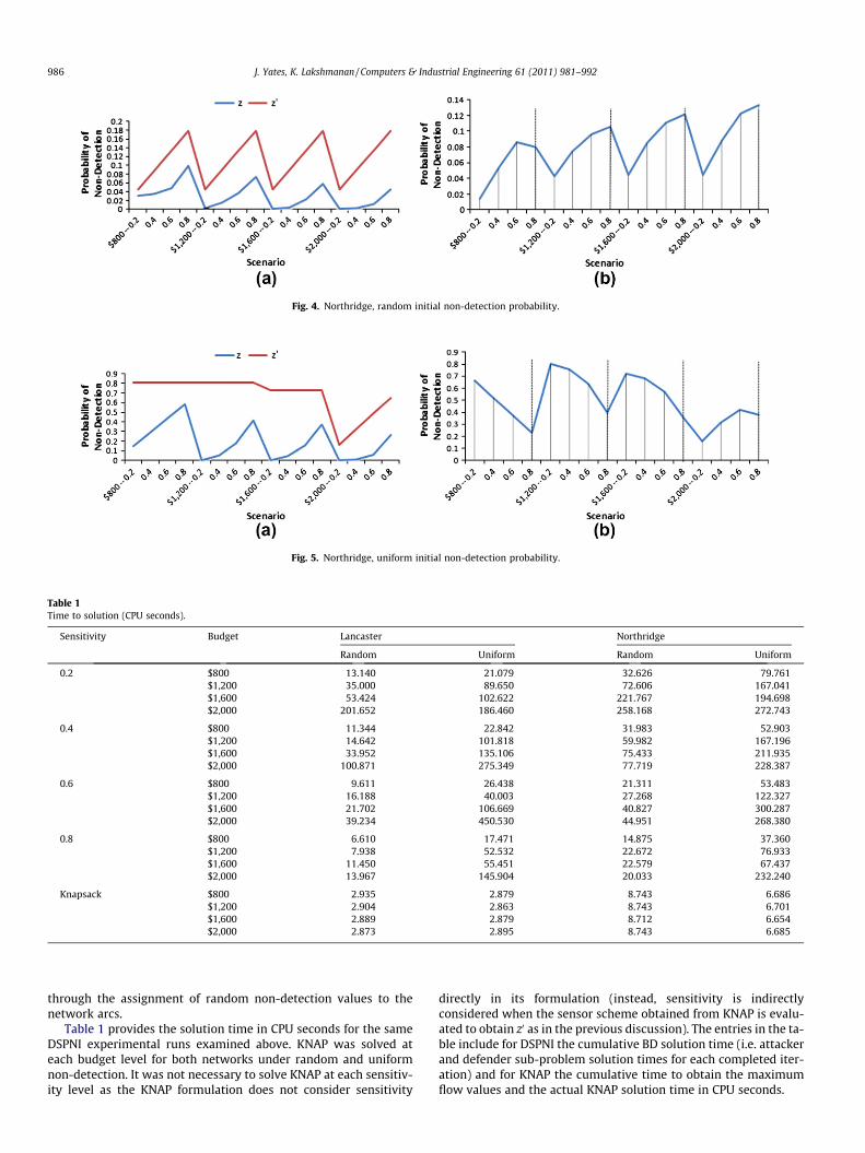
Fig. 4. Northridge, random initial non-detection probability.

Fig. 5. Northridge, uniform initial non-detection probability.

Table 1Time to solution (CPU seconds).

Sensitivity Budget Lancaster Northridge

Random Uniform Random Uniform

0.2 $800 13.140 21.079 32.626 79.761$1,200 35.000 89.650 72.606 167.041$1,600 53.424 102.622 221.767 194.698$2,000 201.652 186.460 258.168 272.743

0.4 $800 11.344 22.842 31.983 52.903$1,200 14.642 101.818 59.982 167.196$1,600 33.952 135.106 75.433 211.935$2,000 100.871 275.349 77.719 228.387

0.6 $800 9.611 26.438 21.311 53.483$1,200 16.188 40.003 27.268 122.327$1,600 21.702 106.669 40.827 300.287$2,000 39.234 450.530 44.951 268.380

0.8 $800 6.610 17.471 14.875 37.360$1,200 7.938 52.532 22.672 76.933$1,600 11.450 55.451 22.579 67.437$2,000 13.967 145.904 20.033 232.240

Knapsack $800 2.935 2.879 8.743 6.686$1,200 2.904 2.863 8.743 6.701$1,600 2.889 2.879 8.712 6.654$2,000 2.873 2.895 8.743 6.685


through the assignment of random non-detection values to thenetwork arcs.

Table 1 provides the solution time in CPU seconds for the sameDSPNI experimental runs examined above. KNAP was solved ateach budget level for both networks under random and uniformnon-detection. It was not necessary to solve KNAP at each sensitiv-ity level as the KNAP formulation does not consider sensitivity

directly in its formulation (instead, sensitivity is indirectlyconsidered when the sensor scheme obtained from KNAP is evalu-ated to obtain z0 as in the previous discussion). The entries in the ta-ble include for DSPNI the cumulative BD solution time (i.e. attackerand defender sub-problem solution times for each completed iter-ation) and for KNAP the cumulative time to obtain the maximumflow values and the actual KNAP solution time in CPU seconds.


Understanding the trends of the experimental networks isimportant when interpreting the values and implications of Table1. Lancaster-Palmdale is a significantly sparser network thanNorthridge with only 216/77 arcs/nodes compared to 386/140arcs/nodes, respectively. In addition, Lancaster-Palmdale occupiesa significantly larger spatial region and required 743 uniformlydistributed atoms for potential sensor locations compared to220 in Northridge. In general, increases in sensitivity and in-creases in budget result in longer computation times to solveDSPNI to optimality using BD. In addition, the uniform initialnon-detection case yields longer CPU seconds for both networksover the random case. Finally, the increased density/complexityof the Northridge network resulted in consistent increases incomputational time for nearly every experimental run. To thecontrary, KNAP was statistically impervious to budgetary changeswhile maintaining comparatively low solutions times for bothnetworks. In practice, obtaining the actual KNAP sensor schemewas performed in under 1 CPU second for both networks withthe increase in CPU time between Lancaster-Palmdale and North-ridge for KNAP stemming from the increased time to obtain arcaggregate maximum flows.

5. Spatial analysis results and discussion

Spatially, the similarity between KNAP and DSPNI was exam-ined using both visualization, statistical and spatial analysis tech-niques. Statistical data was collected on the percentage of atomsused in the DSPNI optimal solution that were captured by theKNAP approximation as well as the percentage of aggregate DSPNInetwork arc coverage captured by the KNAP approximation. DSPNIatom usage and network influence were aggregated across allexperimental runs because the goal of the KNAP is not to approx-imate the solution of a single experimental instance but rather theoverall regional spatial trends in protecting critical infrastructure.Using spatial analysis techniques, raster files of the DSPNI aggre-gate solution and the KNAP approximations were obtained usingkernel density. KNAP performance was determined by examiningthe similarity in kernel density between the KNAP approximationsand the DSPNI solution, with higher similarity indicating a strongerKNAP approximation. Finally, the separate factor levels of theexperimental design were analyzed using statistical techniquesto identify the significant factor levels as well as any potentialinteraction.

Assuming that a policy makers’ primary concern is the alloca-tion of defense resources and not obtainment of the optimal objec-tive solution value, the validity of devised approximationprocedures such as the KNAP approach of this paper must be sup-ported spatially. In other words, for KNAP to be accepted as a rea-sonable approximation method for DSPNI, demonstrable evidenceof the spatial capabilities of KNAP to allocate resources in similarlyto the optimal DSPNI allocations must be presented. As a first ap-proach to validating the KNAP approach, Figs. 6 and 7 are intro-duced. In the figures, the upper-left map illustrates theaggregated DSPNI resource allocation while the upper-right mapshows the maximum flow solution obtained using arc non-detec-tion probabilities as flow capacities. The remaining maps illustrateKNAP allocation solutions obtained for alternate overlap and alphavalues. Fig. 6 presents the solutions for Lancaster-Palmdale andFig. 7 for Northridge. In both figures, budget constrained the allo-cation of sensors to a maximum of 4, 8, 12 and 16 respectively in(a)–(d).

The figures illustrate a visual connection between the aggre-gated frequency of maximum flow and the DSPNI solutions in bothnetworks. Performance of the KNAP approximation also appears tobe consistent under certain budgetary, overlap and alpha levels, in

allocating sensors to areas of high allocation as obtained from solv-ing the DSPNI to optimality.

To further investigate the similarity between DSPNI and KNAPsolutions, a computational study on atom usage and arc coveragewas performed. Table 2 provides a sample of the collected dataused in the analysis. In total, an instance of the KNAP formulationwas solved for each of the following factor level combinations.

� Overlap = {1,2,3,4}� Alpha = {0,0.01,0.02, . . . ,0.98,0.99,1.0}� Budget = {4,8,12,16}

The resulting allocations were then compared to the optimalatom usage and arc influence solutions obtained from solving theDSPNI formulation at the specified budget level (recall that inDSPNI, the decision variable y corresponded to atom usage and cto arc influence). In Table 2, the percentage of DSPNI used atomscaptured by the KNAP formulation is given as %Atoms. The percent-age of DSPNI influenced arcs captured by the KNAP formulation isgiven as %Agg. Table 3 returns the statistical p-value from testingthe null hypothesis that the mean observed values of factor x donot differ. In this case, the examined factors were the networktested (network), random versus uniform initial arc non-detectionprobabilities (rand/unif), allowable overlap in the KNAP formula-tion (overlap), KNAP multi-criteria weight (alpha), DSPNI budgetlevel (budget), sensor sensitivity (sensitivity) and KNAP budget le-vel (k-value).

The analysis performed in Table 2 is rather strict in its interpre-tation, counting only those atoms or arcs in %Atoms and %Aggwhich match exactly between KNAP and DSPNI. Even with such astrict interpretation, the performance of KNAP was encouraging.KNAP was consistently able to identify 20% of the DSPNI atomsused 30–40% of the DSPNI influenced arcs. In Table 3, the percent-age gap between the DSPNI optimal solution and minmax pathnon-detection probability of the KNAP optimal solution behavedconsistently across all measured factors except sensor sensitivity.The objective difference between the two, by contrast, was affectedby network choice and whether initial arc non-detection probabil-ities were random or uniform. This supports the assertion thatKNAP may be an acceptable substitute for DSPNI because its per-centage deviation from the optimal DSPNI objective value doesnot deviate with network connectivity or structure. Additionally,the %Atoms and %Agg, a measure of spatial similarity, were not sta-tistically affected by network selection.

More formally, ArcGIS 9.3 was used to obtain kernel densitiesfor each of the DSPNI and KNAP solutions (kernel density gives val-uation at the raster/cell level to data which is normally vectorbased. See (ESRI, 2009) for additional information on the calcula-tion of kernel density) to assess performance of the KNAP approx-imation. From the kernel density, raster map algebra was used toevaluate the approximation capability of KNAP by comparing thecellular raster density of DSPNI and KNAP solutions. To this extent,four separate comparisons were performed; equality of kernel den-sities (EQ), less than or equality of kernel densities (LessEQ), equal-ity of binary density (B-EQ) and less than or equality of binarydensity (B-LEQ) where binary density refers to a modified kerneldensity where each raster cell is assigned a value of zero if itskernel density is zero and a value of one if its kernel density ispositive. Binary evaluations are used as a method to compensatefor the disparity in kernel density ranges which results fromcomparison of KNAP to aggregated DSPNI solutions which considera larger number of allocated resources (in the case to be describedbelow, the Lancaster-Palmdale DSPNI aggregated resource locationconsiders 112 located resources while KNAP seeks to approximatetheir spatial location by allocating 12 resources to the region). Theminimum, maximum, mean and standard deviations of these

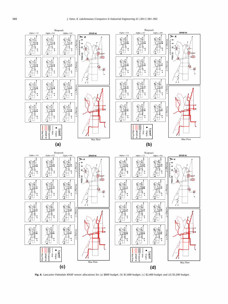
Fig. 6. Lancaster-Palmdale KNAP sensor allocations for (a) $800 budget, (b) $1,600 budget, (c) $2,400 budget and (d) $3,200 budget.


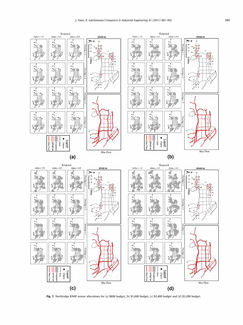
Fig. 7. Northridge KNAP sensor allocations for (a) $800 budget, (b) $1,600 budget, (c) $2,400 budget and (d) $3,200 budget.


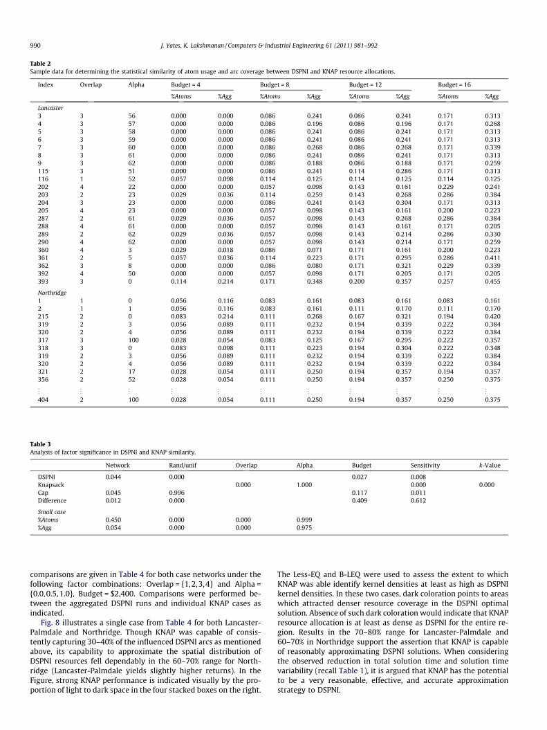
Table 2Sample data for determining the statistical similarity of atom usage and arc coverage between DSPNI and KNAP resource allocations.

Index Overlap Alpha Budget = 4 Budget = 8 Budget = 12 Budget = 16

%Atoms %Agg %Atoms %Agg %Atoms %Agg %Atoms %Agg

Lancaster3 3 56 0.000 0.000 0.086 0.241 0.086 0.241 0.171 0.3134 3 57 0.000 0.000 0.086 0.196 0.086 0.196 0.171 0.2685 3 58 0.000 0.000 0.086 0.241 0.086 0.241 0.171 0.3136 3 59 0.000 0.000 0.086 0.241 0.086 0.241 0.171 0.3137 3 60 0.000 0.000 0.086 0.268 0.086 0.268 0.171 0.3398 3 61 0.000 0.000 0.086 0.241 0.086 0.241 0.171 0.3139 3 62 0.000 0.000 0.086 0.188 0.086 0.188 0.171 0.259115 3 51 0.000 0.000 0.086 0.241 0.114 0.286 0.171 0.313116 1 52 0.057 0.098 0.114 0.125 0.114 0.125 0.114 0.125202 4 22 0.000 0.000 0.057 0.098 0.143 0.161 0.229 0.241203 2 23 0.029 0.036 0.114 0.259 0.143 0.268 0.286 0.384204 3 23 0.000 0.000 0.086 0.241 0.143 0.304 0.171 0.313205 4 23 0.000 0.000 0.057 0.098 0.143 0.161 0.200 0.223287 2 61 0.029 0.036 0.057 0.098 0.143 0.268 0.286 0.384288 4 61 0.000 0.000 0.057 0.098 0.143 0.161 0.171 0.205289 2 62 0.029 0.036 0.057 0.098 0.143 0.214 0.286 0.330290 4 62 0.000 0.000 0.057 0.098 0.143 0.214 0.171 0.259360 4 3 0.029 0.018 0.086 0.071 0.171 0.161 0.200 0.223361 2 5 0.057 0.036 0.114 0.223 0.171 0.295 0.286 0.411362 3 8 0.000 0.000 0.086 0.080 0.171 0.321 0.229 0.339392 4 50 0.000 0.000 0.057 0.098 0.171 0.205 0.171 0.205393 3 0 0.114 0.214 0.171 0.348 0.200 0.357 0.257 0.455

Northridge1 1 0 0.056 0.116 0.083 0.161 0.083 0.161 0.083 0.1612 1 1 0.056 0.116 0.083 0.161 0.111 0.170 0.111 0.170215 2 0 0.083 0.214 0.111 0.268 0.167 0.321 0.194 0.420319 2 3 0.056 0.089 0.111 0.232 0.194 0.339 0.222 0.384320 2 4 0.056 0.089 0.111 0.232 0.194 0.339 0.222 0.384317 3 100 0.028 0.054 0.083 0.125 0.167 0.295 0.222 0.357318 3 0 0.083 0.098 0.111 0.223 0.194 0.304 0.222 0.348319 2 3 0.056 0.089 0.111 0.232 0.194 0.339 0.222 0.384320 2 4 0.056 0.089 0.111 0.232 0.194 0.339 0.222 0.384321 2 17 0.028 0.054 0.111 0.250 0.194 0.357 0.194 0.357356 2 52 0.028 0.054 0.111 0.250 0.194 0.357 0.250 0.375

..

. ... ..

. ... ..

. ... ..

. ... ..

. ... ..

.

404 2 100 0.028 0.054 0.111 0.250 0.194 0.357 0.250 0.375

Table 3Analysis of factor significance in DSPNI and KNAP similarity.

Network Rand/unif Overlap Alpha Budget Sensitivity k-Value

DSPNI 0.044 0.000 0.027 0.008Knapsack 0.000 1.000 0.000 0.000Cap 0.045 0.996 0.117 0.011Difference 0.012 0.000 0.409 0.612

Small case%Atoms 0.450 0.000 0.000 0.999%Agg 0.054 0.000 0.000 0.975


comparisons are given in Table 4 for both case networks under thefollowing factor combinations: Overlap = {1,2,3,4} and Alpha ={0.0,0.5,1.0}, Budget = $2,400. Comparisons were performed be-tween the aggregated DSPNI runs and individual KNAP cases asindicated.

Fig. 8 illustrates a single case from Table 4 for both Lancaster-Palmdale and Northridge. Though KNAP was capable of consis-tently capturing 30–40% of the influenced DSPNI arcs as mentionedabove, its capability to approximate the spatial distribution ofDSPNI resources fell dependably in the 60–70% range for North-ridge (Lancaster-Palmdale yields slightly higher returns). In theFigure, strong KNAP performance is indicated visually by the pro-portion of light to dark space in the four stacked boxes on the right.

The Less-EQ and B-LEQ were used to assess the extent to whichKNAP was able identify kernel densities at least as high as DSPNIkernel densities. In these two cases, dark coloration points to areaswhich attracted denser resource coverage in the DSPNI optimalsolution. Absence of such dark coloration would indicate that KNAPresource allocation is at least as dense as DSPNI for the entire re-gion. Results in the 70–80% range for Lancaster-Palmdale and60–70% in Northridge support the assertion that KNAP is capableof reasonably approximating DSPNI solutions. When consideringthe observed reduction in total solution time and solution timevariability (recall Table 1), it is argued that KNAP has the potentialto be a very reasonable, effective, and accurate approximationstrategy to DSPNI.

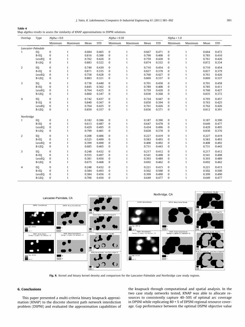
Table 4Map algebra results to assess the similarity of KNAP approximations to DSPNI solutions.

Overlap Type Alpha = 0.0 Alpha = 0.50 Alpha = 1.0

Minimum Maximum Mean STD Minimum Maximum Mean STD Minimum Maximum Mean STD

Lancaster-Palmdale1 EQ 0 1 0.684 0.465 0 1 0.667 0.471 0 1 0.664 0.472

B-EQ 0 1 0.816 0.388 0 1 0.790 0.408 0 1 0.785 0.410LessEQ 0 1 0.762 0.426 0 1 0.759 0.428 0 1 0.761 0.426B-LEQ 0 1 0.883 0.322 0 1 0.874 0.332 0 1 0.872 0.334

2 EQ 0 1 0.740 0.439 0 1 0.710 0.454 0 1 0.710 0.454B-EQ 0 1 0.871 0.335 0 1 0.827 0.378 0 1 0.827 0.379LessEQ 0 1 0.758 0.428 0 1 0.760 0.427 0 1 0.761 0.426B-LEQ 0 1 0.883 0.321 0 1 0.869 0.337 0 1 0.869 0.337



Northridge1 EQ 0 1 0.182 0.386 0 1 0.187 0.390 0 1 0.187 0.390

B-EQ 0 1 0.613 0.487 0 1 0.647 0.478 0 1 0.649 0.477LessEQ 0 1 0.429 0.495 0 1 0.434 0.496 0 1 0.429 0.495B-LEQ 0 1 0.799 0.401 0 1 0.828 0.378 0 1 0.830 0.376




Fig. 8. Kernel and binary kernel density and comparison for the Lancaster-Palmdale and Northridge case study regions.


6. Conclusions

This paper presented a multi-criteria binary knapsack approxi-mation (KNAP) to the discrete shortest path network interdictionproblem (DSPNI) and evaluated the approximation capabilities of

the knapsack through computational and spatial analysis. In thetwo case study networks tested, KNAP was able to allocate re-sources to consistently capture 40–50% of optimal arc coveragein DPSNI while replicating 80 + % of DPSNI regional resource cover-age. Gap performance between the optimal DSPNI objective value


and the corresponding objective value under KNAP resource alloca-tion was statistically consistent in both networks with a 95% con-fidence interval. Additionally, it was shown that the multiplecriteria considered in the KNAP objective (aggregate maximumflow and distance from the closest origin) did not significantly im-pact KNAP approximation capabilities. Implementing KNAP in lieuof DSPNI, therefore, maintains spatial integrity in the obtainedoptimal solutions while requiring comparatively reduced compu-tational burden. Such a result becomes particularly important asnetwork size increases and the DSPNI problem becomes computa-tionally intractable. In these cases, approximation methods such asKNAP can be used to support test-case analysis and what-if analy-sis for a myriad of scenarios in the determination of policy and re-source allocation for decision-makers or to examine regions andnetworks previously too large/complex to solve using traditionalDSPNI solution methods.

References

Balcioglu, A., & Wood, R. K. (2003). Enumerating near-min s-t cuts. In D. L. Woodruff(Ed.), Network interdiction and stochastic integer programming (pp. 51–69).Boston: Academic Publishers.

Bard, Jonathan (1998). Practical bilevel optimization: Algorithms and applications.Boston: Kluwer Academic Publishers.

Boyle, M. R. (1998). partial-enumeration for planarnetwork interdiction problems.M.S. thesis.

Brown, G., Carlyle, M., Salmeron, J., & Wood, K. (2006). Defending criticalinfrastructure. Interfaces, 36(6), 530–544.

Burch, C., Carr, R., Krumke, S., Marathe, M., Phillips, C., & Sundberg, E. (2003). Adecomposition-based approximation for network inhibition. In Networkinterdiction and stochastic programming (pp. 51–69). Boston: Kluwer AcademicPublishers.

Church, R., & Scaparra, M. P. (2007). Protecting critical assests: The r-interdictionmedian problem with fortification. Geographical Analysis, 39, 129–146.

Corley, H. W., & Chang, H. (1974). Finding the n most vital nodes in a flow network.Management Science, 21, 362–364.

Cunningham, W. H. (1985). Optimal attack and reinforcement of a network. Journalof the Association for Computing Machinery, 32(3), 549–561.

ESRI. (2009). ArcGIS: A complete integrated system. http://www.esri.com/software/arcgis/index.html. Accessed 10.02.10.

Ford, L. R., & Fulkerson, D. R. (1962). Flows in networks. Princeton Press.Ghare, P., Montgomery, D., & Turner, W. C. (1971). Optimal interdiction policy for a

flow network. Naval Research Logistics Quarterly, 18, 37–45.Held, H., & Woodruff, D. (2005). Heuristics for multi-stage interdiction of stochastic

networks. Journal of Heuristics, 11, 483–500.Israeli, E., & Wood, K. (2002). Shortest-path network interdiction. Networks, 40(2),

97–111.Lim, C., & Smith, J. C. (2007). Algorithms for discrete and continuous

multicommodity flow network interdiction problems. IIE Transactions, 39,15–26.

Matisziw, T., Murray, A., & Grubesic, T. (2007). Bounding network interdictionvulnerability through cut-set identification. In Advancing spatial science (pp.243–255).

Nemhauser, G., & Wolsey, L. (1999). Integer and combinatorial optimization. NewYork: Wiley-Interscience.

Phillips, C. A. (1993). The network inhibition problem. In Proceedings of the annualassociation for computer machinery STOC.

Ratliff, H. D., Sicilia, G., & Lubore, S. (1975). Finding the n most vital links in flownetworks. Management Science, 21(5), 539–631.

Royset, J., & Wood, R. K. (2007). Solving the bi-objective maximum-flow network-interdiction problem. INFORMS Journal on Computing, 19(2), 175–184.

Salmeron, J., Wood, R. K., & Baldick, R. (unpublished). Analysis of electric gridsecurity under terrorist threat.

US Census Bureau. (2008). TIGER/Line and TIGER-related products. <http://www.census.gov/geo/www/tiger/> Accessed 01.08.08.

Wollmer, R. (1964). Removing arcs from a network. Operations Research, 12,934–940.

Wood, R. K. (2003). Deterministic network interdiction. Mathematical ComputerModeling, 17(2), 1–18.

Yates, Justin, & Casas, Irene (2010). Role of spatial data in the protection of criticalinfrastructure and homeland defense. Applied Spatial Analysis and Policy, 1–18.

http://www.esri.com/software/arcgis/index.html

http://www.esri.com/software/arcgis/index.html

http://www.census.gov/geo/www/tiger/

http://www.census.gov/geo/www/tiger/

Documents

A constrained binary knapsack approximation for shortest path network interdiction