Embed Size (px)
Citation preview

A decision support system for managing irrigation in agriculture
Navarro Hellin, H., Martínez-del-Rincon, J., Domingo Miguel, R., Soto Valles, F., & Torres Sanchez, R. (2016). Adecision support system for managing irrigation in agriculture. Computers and Electronics in Agriculture, 124,121-131. DOI: 10.1016/j.compag.2016.04.003
Published in:Computers and Electronics in Agriculture
Document Version:Peer reviewed version
Queen's University Belfast - Research Portal:Link to publication record in Queen's University Belfast Research Portal
Publisher rights© 2016 Elsevier B. V. This manuscript version is made available under the CC-BY-NC-ND 4.0licensehttp://creativecommons.org/licenses/by-nc-nd/4.0/,which permits distribution and reproduction for non-commercial purposes, providedthe author and source are cited.
General rightsCopyright for the publications made accessible via the Queen's University Belfast Research Portal is retained by the author(s) and / or othercopyright owners and it is a condition of accessing these publications that users recognise and abide by the legal requirements associatedwith these rights.
Take down policyThe Research Portal is Queen's institutional repository that provides access to Queen's research output. Every effort has been made toensure that content in the Research Portal does not infringe any person's rights, or applicable UK laws. If you discover content in theResearch Portal that you believe breaches copyright or violates any law, please contact [email protected].
Download date:13. Oct. 2018

1
A Decision Support System for managing irrigation in 1
agriculture 2
H. Navarro-Hellína, J. Martínez-del-Rinconb, R. Domingo-Miguelc, 3
F. Soto-Vallesd and R. Torres-Sáncheze* 4
a Widhoc Smart Solutions S.L. Parque Tecnológico de Fuente Álamo, CEDIT. Carretera del 5
Estrecho-Lobosillo Km 2 30320, Fuente Álamo. (Murcia), Spain. 6
b The Institute of Electronics, Communications and Information Technology (ECIT), Queens 7
University of Belfast, Belfast BT3 9DT, UK 8
c Producción Vegetal Department, Universidad Politécnica de Cartagena, Paseo Alfonso XIII, 48 9
30203, Cartagena (Murcia), Spain 10
d Tecnología Electrónica Department, Universidad Politécnica de Cartagena, Campus Muralla del 11
Mar, Doctor Fleming, s/n 30202, Cartagena (Murcia), Spain 12
e Ingeniería de Sistemas y Automática Department, Universidad Politécnica de Cartagena, 13
Campus Muralla del Mar, Doctor Fleming, s/n 30202, Cartagena (Murcia), Spain 14
15
*Corresponding author at: Ingeniería de Sistemas y Automática Department, Universidad 16
Politécnica de Cartagena, Campus Muralla del Mar, Doctor Fleming, s/n 30202, Cartagena 17
(Murcia), Spain. 18
Tel.: +34 968 325 474 19
E-mail address: [email protected] 20
21
*ManuscriptClick here to view linked References
2
Abstract 22
In this paper, an automatic Smart Irrigation Decision Support System, SIDSS, is proposed to 23
manage irrigation in agriculture. Our system estimates the weekly irrigations needs of a 24
plantation, on the basis of both soil measurements and climatic variables gathered by several 25
autonomous nodes deployed in field. This enables a closed loop control scheme to adapt the 26
decision support system to local perturbations and estimation errors. Two machine learning 27
techniques, PLSR and ANFIS, are proposed as reasoning engine of our SIDSS. Our approach is 28
validated on three commercial plantations of citrus trees located in the South-East of Spain. 29
Performance is tested against decisions taken by a human expert. 30
Keywords: Irrigation, Decision Support System, water optimization, machine learning. 31
32
33
The efficient use of water in agriculture is one of the most important agricultural challenges that 34
modern technologies are helping to achieve. In arid and semiarid regions, the differences between 35
precipitation and irrigation water requirements are so big that irrigation management is a priority 36
for sustainable and economically profitable crops (IDAE, 2005). 37
To accomplish this efficient use, expert agronomists rely on information from several sources 38
(soil, plant and atmosphere) to properly manage the irrigation requirements of the crops (Puerto 39
et al., 2013). This information is defined by a set of variables, which can be measured using 40
sensors, that are able to characterise the water status of the plants and the soil in order to obtain 41
their water requirements. While meteorological variables are representative of a large area and 42

3
can be easily measured by a single sensor for a vast land extension, soil and plant variables have 43
a large spatial variability. Therefore, in order to use these parameters to effectively schedule the 44
irrigation of the plants, multiple sensors are needed (Naor et al., 2001). 45
Weather is one of the key factors being used to estimate the water requirements of the crops 46
(Allen et al., 1998). Moreover, it is very frequent that public agronomic management organisms 47
have weather stations spread around the different regions. These weather stations usually provide 48
information of key variables for the agriculture like reference evapotranspiration (ET0) or the 49
Vapour Pressure Deficit (VPD) that are of great importance to calculate the water requirements 50
of the crops. Using variables related to the climate is the most common approach to create crop 51
water requirement models (Jensen et al., 1970; Smith, 2000; Zwart and Bastiaanssen, 2004). 52
Using these models, based on solely meteorological variables, a decision-making system can 53
determine how a given crop will behave (Guariso et al., 1985). 54
However, not all the regions have access to an extensive network of weather stations or they may 55
not be nearby a given crop, thus the local micro-climates are not taken into account if only these 56
parameters are used. Besides, irrigation models based only on climate parameters rely on an open 57
loop structure. This means that the model is subject to stochastic events and it may not be able to 58
correct the local perturbations that can occur when a unexpected weather phenomenon occurs (for 59
(Dutta et al., 2014; Giusti and Marsili-Libelli, 60
2015). Finally, monitoring other variables, such as hydrodynamic soil factors or water drainage, 61
might increase the chances that the irrigation predicted by the models is properly used by the 62
plants (Kramer and Boyer, 1995). Therefore, the usage of sensors that measures the soil water 63
status is a key complement to modulate the water requirements of the crops. Soil variables, such 64

4
as soil moisture content or soil matric potential, are considered by many authors as crucial part of 65
scheduling tools for managing irrigation (Cardenas-Lailhacar and Dukes, 2010; Soulis et al., 66
2015). The information from soil sensors can be used to create better decision models with closed 67
loop structures that adapt to weather and soil perturbations (Cardenas-Lailhacar and Dukes, 2010; 68
Soulis et al., 2015). This practice, however, has not been widely adopted due to the technological 69
limitations of available soil sensors, which required measured information to be registered and 70
stored, traditionally using wired dataloggers, and limiting the installation flexibility and the real 71
time interaction. This has changed recently with new generation sensors and sensor networks that 72
are more versatile and suited to the agricultural environment (Navarro-Hellín et al., 2015). 73
Combining climate and soil variables has therefore potential to properly manage irrigation in a 74
more efficient way than other traditional approaches. However, it also entails a series of 75
challenges related with the increased amount of data flow, its analysis and its use to create 76
effective models, in particular when data provided by different sources may seem contradictory 77
and/or redundant. Traditionally, this analysis and modelling is performed by a human expert who 78
interprets the different variables. The need of a human agronomist expert is required due to the 79
complexity introduced by the soil spatial variability, crop species variability and their irrigation 80
requirements over the growth cycle (Maton et al., 2005), which require comparing crops models 81
and local context variables to determine the specific water requirements to achieve a certain goal 82
at a particular location. 83
The complexity of this problem and the different sources of variability makes than even the best 84
model may deviate from the prediction, which favours the use of close loop control systems 85

5
combining soil and climate sensors over open loop systems as a way to compensate possible 86
deviations in future predictions. 87
Human expertise has been proved effective to assist irrigation management but it is not scalable 88
and available to every field, farm and crop and it is slow in the analysis of the data and real time 89
processing. Instead, applying machine learning techniques to replace the manual models and to 90
assist expert agronomists allows the viability of creating automatic Irrigation Decision Support 91
System. Machine learning techniques have been used previously to estimate relevant parameters 92
of the crop (Sreekanth et al., 2015). Giusti and Marsili-Libelli(2015) present a fuzzy decision 93
systems to predict the volumetric water content of the soil based on local climate data. Adeloye 94
et al. (2012), proposed the use of unsupervised artificial neural networks (ANN) to estimate the 95
evapotranspiration also based on weather information solely. King and Shellie (2016) used NN 96
modelling to estimate the lower threshold temperature (Tnws) needed to calculate the crop water 97
stress index for wine grapes. In Campos et al. (2016) the authors presented a new algorithm 98
designed to estimate the total available water in the soil root zone of a vineyard crop, using only 99
SWC sensors, which are very dependent of the location. Taking advantage of the soil 100
information, Valdes-Vela et al.(2015) and Abrisqueta et al.(2015) incorporates the volumetric 101
soil water content, manually collected with a neutron probe, to agro-meteorological data. This 102
information is then fed into a fuzzy logic system to estimate the stem water potential. Other 103
approaches in the literature also make use of machine learning techniques -such as principal 104
component analysis, unsupervised clustering, ANN, etc.- to estimate the irrigation requirements 105
in crops. However they do not specify the quantity of water needed (Dutta et al., 2014), they 106
reduce the prediction to true or false, and/or they are based on open loop structures (Giusti and 107

6
Marsili-Libelli, 2015; Jensen et al., 1970; Smith, 2000; Zwart and Bastiaanssen, 2004), only 108
considering the weather information and, therefore, unable to correct deviations from their 109
predictions. 110
This paper proposes an automated decision support system to manage the irrigation on a certain 111
crop field, based on both climatic and soil variables provided by weather stations and soil 112
sensors. As discussed, we postulate that the usage of machine learning techniques with the 113
weather and soil variables is of great importance and can help to achieve a fully automated close 114
loop system able to precisely predict the irrigation needs of a crop. Our presented system is 115
evaluated by comparing it against the irrigations reports provided by an agronomist specialist 116
during a complete season in different fields. 117
118
An irrigation advice system is based on the concept of predicting the waters needs of the crops in 119
order to irrigate them properly. Traditionally this decision has been taken by an experienced 120
farmer or an expert agricultural technician. Figure 1 shows the flow diagram of which the 121
proposed system is based. 122
In this schema, an expert agronomist is in charge of analysing the information from different 123
sources: Weather stations located near the crops that collect meteorological data, Crop and Soil 124
characteristics (type, age, size, cycle, etc.) and Soil sensors installed in the crop fields. The expert 125
analyses the information to provide an irrigation report, which indicates the amount of water 126
needed to irrigate properly the crops in the upcoming week. To make this decision making 127
7
process manageable, the information needed to create the irrigation report on the next week is 128
only the information of the current week. 129
130
Figure 1: Flow Diagram of the proposed system 131
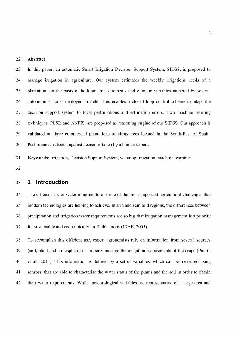
Based on this concept, our Smart Irrigation Decision Support System (SIDSS) is proposed. In 132
order to evaluate the performance and validity of our approach, the decision system will use the 133
same information used by the expert agronomist and will output the water requirements for the 134
upcoming week. This will ensure a fair comparison between the decisions taken by a human 135
expert and the SIDSS. To accomplish this, the machine learning system must be trained with 136
historical data and irrigations reports of the agronomist, using the irrigation decisions taken in 137
these reports as the groundtruth of the system. The aim of the system is to be as accurate as 138
possible to this groundtruth. Several machine learning techniques were applied and evaluated to 139
achieve the best performance. Figure 2 shows a diagram of the SIDSS. 140
The Irrigation Decision System is composed of three main components: a collection device that 141
gathers information from the soil sensors, weather stations that provide agrometeorological 142
information and the SIDSS that, when trained correctly, is able to predict the irrigation 143
8
requirements of the crops for the incoming week. Table 1 shows the set of possible input 144
variables of the system. 145
146
Figure 2: Training inputs and targets of SIDSS 147
Table 1: Set of possible input variables of the system 148

9
149
The information from the soil sensors is gathered using our own developed device that has been 150
proved to be completely functional for irrigation management in different crops and conditions 151
(Navarro-Hellin et al., 2015). This device is wireless, equipped with a GSM/GPRS modem, and 152
is completely autonomous, so that the installation procedures are accessible to any farmer. 153
Figure 3 shows the collection device installed in a lemon crop field located in the South-East of 154
Spain. 155
156
Figure 3: Device installed in a lemon crop field. 157
The device allows to fully configure the recording rates of all the embedded sensors. In our 158
experiments, a sampling rate of 15 minutes was set, since this gives a good balance between 159
providing enough information to support a correct agronomic decision and maintaining the 160

10
autonomy of the device with the equipped solar panel and battery (López Riquelme et al., 2009; 161
Navarro-Hellin et al., 2015). The information is received, processed and stored in a relational 162
database. 163
2.1.1. Soil Sensors 164
The soil control variables used to provide SIDSS with relevant information are matric potential 165
( m) and volumetric soil water content ( v), which are common in irrigation management (Jones, 166
2004). By using these variables, the irrigation can be scheduled for maintaining soil moisture 167
conditions equivalent or close to field capacity in order to satisfy the required crop water 168
requirements. Likewise, they can be used to maintain soil water content or soil matric potential 169
under certain reference values proper of regulated deficit irrigation strategies. Both m and v are 170
used to decide the irrigation frequency and to adjust the gross irrigation doses. 171
Soil matric potential was measured with MPS-2 sensors (Decagon devices, Inc., Pullman, WA 172
99163 - USA), while volumetric soil water content was measured with both 10-HS (Decagon 173
devices, Inc., Pullman, WA 99163 - USA) and Enviroscan (Sentek Pty. Ltd., Adelaide, Australia) 174
sensors 175
Besides both previous soil sensors, another sensor is used. A pluviometer (Rain-o173-matic 176
small, Pronamic Ltd., Ringkøbing, Denmark) was used under the dripper to provide accurate 177
estimation of the amount of water applied and the irrigation run time. The information provided 178
by this sensor was used to ensure that the farmer is following the instruction of the agronomic 179
reports provided by the expert. Table 2 summarizes the variables measured by the soils sensors. 180
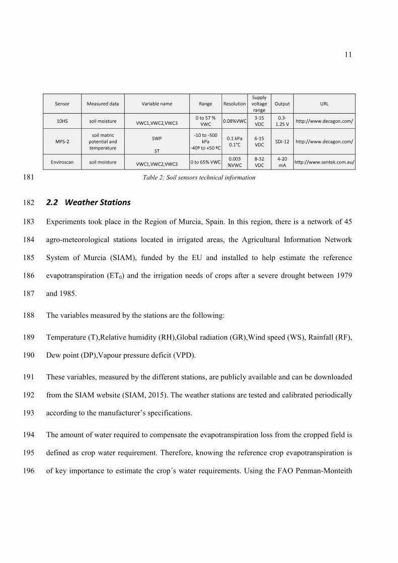
11
Table 2: Soil sensors technical information 181
182
Experiments took place in the Region of Murcia, Spain. In this region, there is a network of 45 183
agro-meteorological stations located in irrigated areas, the Agricultural Information Network 184
System of Murcia (SIAM), funded by the EU and installed to help estimate the reference 185
evapotranspiration (ET0) and the irrigation needs of crops after a severe drought between 1979 186
and 1985. 187
The variables measured by the stations are the following: 188
Temperature (T),Relative humidity (RH),Global radiation (GR),Wind speed (WS), Rainfall (RF), 189
Dew point (DP),Vapour pressure deficit (VPD). 190
These variables, measured by the different stations, are publicly available and can be downloaded 191
from the SIAM website (SIAM, 2015). The weather stations are tested and calibrated periodically 192
according to the manufacturer specifications. 193
The amount of water required to compensate the evapotranspiration loss from the cropped field is 194
defined as crop water requirement. Therefore, knowing the reference crop evapotranspiration is 195
of key importance to estimate the crop´s water requirements. Using the FAO Penman-Monteith 196

12
formulation (Allen et al., 1998), the daily reference crop evapotranspiration (ET0) can be 197
calculated by means of the weather information. The crop evapotranspiration under standard 198
condition (ETc) can be calculated using the single crop coefficient approach shown below: 199
[1] 200
where Kc is the crop coefficient and depends on multiple factors, namely, the crop type, climate, 201
crop evaporation and soil growth stages. 202
203
The decision support system is the component in charge of taking the final decision on the 204
amount of water to be irrigated, or equivalently, the number of minutes to irrigate considering 205
constant water flow. This decision is taken automatically on the basis of the information provided 206
by the sensors and the usage of machine learning and pattern recognition techniques. The aim of 207
this component, therefore, is to mimic a human expert in the decision making process of weekly 208
optimising the irrigation, which could assist the farmer. 209
Applying machine learning techniques such as Principal Component Analysis (PCA) or Linear 210
Discriminant Analysis (LDA) allow us to visualize the information to perform an initial 211
exploratory analysis. Figure 4 shows the LDA of the input, array containing the sensorial 212
variables, and output, the estimated irrigation time need, used in the system. The output was 213
divided in classes (18), each one representing the weekly irrigation time by increments of 150 214
minutes, from 0 to 2,700 minutes. From this figure, it can be noticed that discrete classification in 215
classes will be hard to accomplish due to the high number of classes necessary to precisely 216
quantise the irrigation estimation. This is due to the fact that the variable to estimate - either the 217
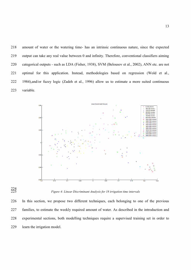
13
amount of water or the watering time- has an intrinsic continuous nature, since the expected 218
output can take any real value between 0 and infinity. Therefore, conventional classifiers aiming 219
categorical outputs - such as LDA (Fisher, 1938), SVM (Belousov et al., 2002), ANN etc. are not 220
optimal for this application. Instead, methodologies based on regression (Wold et al., 221
1984),and/or fuzzy logic (Zadeh et al., 1996) allow us to estimate a more suited continuous 222
variable. 223
224 Figure 4: Linear Discriminant Analysis for 18 irrigation time intervals 225
In this section, we propose two different techniques, each belonging to one of the previous 226
families, to estimate the weekly required amount of water. As described in the introduction and 227
experimental sections, both modelling techniques require a supervised training set in order to 228
learn the irrigation model. 229
14
2.3.1. Partial Least Square Regression 230
Partial Least Square Regression (PLSR) (Wold et al., 2001) is a statistical method that seeks the 231
fundamental relations between predictor and response variables. Predictor variables, X, are 232
defined as the observable variables that can be measured and input into the decision system. 233
Response variable Y are the outputs or estimates that must be deducted from the input. 234
The relationship between both variable sets, and linear multivariate regression model, is found by 235
projecting both predicted and observable variables into a new space, where latent variables are 236
estimated to model the covariance structure between the predictor space and the observation 237
space. 238
This PLSR model is developed from a training set D={X, Y} of S samples, which is composed of 239
the predictor matrix X=[x1, ..xi,..xS]T and the response matrix Y=[y1, ..yi,..yS]
T. xi is a column 240
vector of K elements, that can contain all the sensor and weather variables measured at a given 241
week i: 242
xi=[VWC1,VWC2,VWC3,MP,ST, ETc ,RF,WS,T,RH,GR,DP,VPD]T [2] 243
and yi is another column vector of M elements, containing the corresponding variables to be 244
estimated at that week i. Since in our application this is only the irrigation time recommended at 245
that week, yi is reduced to a scalar and M=1: 246
yi=minutes of irrigation 247
PLSR constructs new predictor latent variables, known as components, which are linear 248
combinations of the original predictor observable variables. These components are created to 249
explain the observed variability in the original predictor variables, while simultaneously 250

15
considering the response variable. That is, the estimated latent variables are linear combinations 251
of predictor variables that have higher covariance with Y. Using the latent variables leads to a 252
regression models able to fit the response variable with fewer components. 253
The PLSR learning model can be expressed as: 254
[3] 255
[4] 256
where T and U are the projections -aka scores- of X and Y into a smaller L-dimensional latent 257
space respectively, P and Q are the orthogonal projection matrices -aka loading matrices- and E 258
and G the error residuals. P and Q can be obtained by eigendecomposition of the original 259
matrices. 260
Since the X-scores T are meant to be good predictors of Y, it can be approximated that: 261
[5] 262
Being F a new residual. This reduces the problem to find a set of weights W such that T=X*W 263
predicts X and Y reasonably well. As mentioned, these orthogonal coefficients should maximise 264
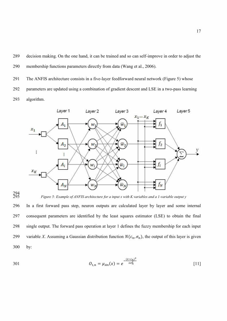
the correlation between X and Y while explaining the variance of X: 265
[6] 266
P and Q can be solved by applying a Least Square Estimator(LSE) so: 267
[7] 268
[8] 269

16
Finally, by rewriting the previous equation, it can be derived that: 270
[9] 271
Being B the PLSR regression coefficients. Once these coefficients have been learned, responses 272
y* for new observation x* can be estimated by applying the learning model: 273
[10] 274
assuming an estimation error f. 275
We favour the use of PLSR among other regression techniques due to its suitability when the 276
number of predictors is bigger than the number of response variables, the responses are noisy and 277
there is a high probability of having multicollinearity among the predictor variables. The 278
multicollinear phenomenon happens when those variable are highly correlated, due to 279
redundancy between sensors and or between meteorological factors. As it can be noticed, all 280
these factors appear in our irrigation problem. 281
282
2.3.2. Adaptive Neuro Fuzzy Inference Systems 283
Adaptive Neuro Fuzzy Inference Systems (ANFIS) (Jang, 1993) is a fuzzy inference system for 284
systematically generating fuzzy rules from a given input/output D dataset. This machine learning 285
technique combines advantages from fuzzy logic and artificial neural networks. On the one hand, 286
it allows us to represent an element not only into categories but also into a certain degree of 287
membership functions, which allows mimicking the characteristics of human reasoning and 288
17
decision making. On the one hand, it can be trained and so can self-improve in order to adjust the 289
membership functions parameters directly from data (Wang et al., 2006). 290
The ANFIS architecture consists in a five-layer feedforward neural network (Figure 5) whose 291
parameters are updated using a combination of gradient descent and LSE in a two-pass learning 292
algorithm. 293
294 Figure 5: Example of ANFIS architecture for a input x with K variables and a 1-variable output y 295
In a first forward pass step, neuron outputs are calculated layer by layer and some internal 296
consequent parameters are identified by the least squares estimator (LSE) to obtain the final 297
single output. The forward pass operation at layer 1 defines the fuzzy membership for each input 298
variable X. Assuming a Gaussian distribution function , the output of this layer is given 299
by: 300
[11] 301
18
Layer 2 is a multiplicative layer, which calculates the firing strength of the rules as a product of 302
the previous membership grades. 303
[12] 304
Layer 3 is a normalising layer, where: 305
[13] 306
Layer 4 applies a node function: 307
[14] 308
where and are consequent parameters estimated using LSE 309
Finally, layer 5 is the output layer that provides the overall estimation y as a summation of all 310
incoming signals. For the case M=1, where only one output variable is estimated: 311
[15] 312
After the forward pass has been completed, an initial estimation is provided by the ANFIS 313
network. Since initial premise parameters are initialised randomly, the initial estimation 314
will differ greatly from the desired values Y. This error or difference between the desired output y 315
and the estimated output for a given training sample { can be expressed as: 316
[16] 317
To correct this deviation, a second learning step, or backward pass, attempts to minimise the 318
estimated error by modifying the value of the premise parameters until the desired and estimated 319
outputs are similar. This process is performed using backpropagation, where the error is 320
19
propagated back over the layers and decomposed into the different nodes using the chain rule. 321
Gradient descend is used as optimisation technique to update the premise parameters while the 322
consequent parameters are kept fixed until the next iteration. 323
This double step learning process is repeated iteratively for every single sample in the training set 324
until the estimated error is smaller than a given threshold, i.e. convergence is achieved, or a 325
maximum number of iterations epocs- are reached. The ANFIS implementation used in this 326
work is taken from the Fuzzy logic toolbox (Inc, 2016), by Mathworks where the parameter Radii 327
used to train was a scalar of value 0.75 and the average number of epochs used to train was 1500. 328
329
The system was evaluated in three commercial plantations of lemon trees in the Region of 330
Murcia, located in the semiarid zone of the South-East of Spain where the water is very scarce 331
and drip irrigation is commonly used. The irrigation criteria followed was to maximize the yield. 332
Plantation 1. Fino lemon trees (Citrus limon L. Burm. fil cv. 49) on C. macrophylla Wester, 333
growing in a soil with a low water retention capacity. The soil is characterized by a deep and 334
homogeneous sandy - clay - loam texture. The irrigation water had an electrical conductivity 335
(EC) of 2200 S cm-1. The orchard consist of 11 year old lemon trees with an average height of 336
3.5 m. Tree spacing was 7.0 m x 5.5 m, with an average ground coverage of about 47%. Two drip 337
irrigation lines (0.8 m apart) were used for each tree row. There were 4 emitters (4 L h-1) on both 338
sides of each tree. One sensor node was installed in the 5.5 ha orchard, with a soil matric 339
potential sensor (MPS-2, Decagon devices, Inc., Pullman, WA 99163 - USA) at a depth of 30 cm 340

20
and three soil moisture sensors at a depth of 20, 40 and 80 cm (Enviroscan, Sentek Pty. Ltd., 341
Adelaide, Australia) located 20 cm from a representative dripper and 2.25 m from the trunk. 342
According to the nearest weather station of SIAM, located about 5 km from the orchard, the 343
climate was typically Mediterranean. Thus, over this period (2014), the annual rainfall for the 344
area was 210 mm and ET0 was 1395 mm. The average wind speed was 1.66 m/s, generally light 345
wind and sometimes moderate. 346
Plantation 2 and 3. 40 and 35 year old lemon trees (Citrus limon L. Burm. Fil) cv. Fino and cv. 347
Verna respectively, grafted on sour orange (Citrus aurantium L.), growing in a soil with a 348
medium water retention capacity. The soil is clay sandy loam texture and the irrigation water had 349
an electrical conductivity (EC) of 1600 S cm-1 during all season except in summer which was of 350
2285 S cm-1. The tree spacing was 7.0 m x 6.75 m and 6.75 m x 6.75 m and the average ground 351
coverage about 57% and 50%, respectively. One drip irrigation line was used for each tree row. 352
There were 8 and 6 emitters of 4 L h-1 per tree, respectively. One sensor node was installed in the 353
Fino orchard ( 15 ha) and another in Verna orchard ( 23 ha), each with two soil matric potential 354
sensor (MPS-2, Decagon devices, Inc., Pullman, WA 99163 - USA) at a depth of 25 and 45 cm 355
and three soil moisture sensors at a depth of 25, 45 and 70 cm (10HS, Decagon devices, Inc., 356
Pullman, WA 99163) located 20 cm from a representative dripper and the vertical canopy 357
projection. 358
359
climate was also typically Mediterranean. Over this period (2014), the annual rainfall for the area 360

21
was 150 mm and ET0 was 1250 mm. The average wind speed was 1.4 m s-1, i.e. light wind 361
generally. 362
The decision of selecting these three plantations is based on the fact that all of them are mature 363
lemon trees and therefore their water irrigation requirement differences depend mainly of 364
environmental conditions (soil and atmosphere) rather than the plant. Besides, all the plantations 365
use drip emitters of 4 L h-1 so estimating the irrigation runtime of the week instead of the water 366
volume will be a correct approach. 367
Drip irrigation provides a fixed volume of water per hour; the pressure is maintained using 368
pressure compensating emitters. The Irrigation frequency is calculated taking into account that 369
only a certain amount of water depletion is allowed before the next replenishment is scheduled. 370
Thus, the run time (gross irrigation dose) is determined to be equivalent to the previous amount 371
of water depletion. The experts only need to calculate the irrigation run time (minutes) and the 372
number of watering times per week or day depending on the time of year or crop development 373
stage. The main goal of the system, also reflected by the expert agronomist in his reports, is to 374
maximize the yield (maximum production per crop surface) with an optimum water management. 375
Since information from the weather stations, soil sensors and crops characteristics has different 376
sampling periods, the first step is pre-process this information. After analysing several methods 377
and time intervals it was decided that the best option was to calculate the week average value for 378
each of the sensors or weather stations variable except for the rainfall where the total amount of 379
rainfall during the week is used instead. The week average fits better than others method like the 380
daily average due to the fact, that the irrigation reports from the expert agronomist are already 381
fixed, limited and done weekly. Besides, adding more input will make the data sparser, making 382

22
more difficult to find patterns in the feature space, requiring a higher amount of data to train the 383
system accordingly. 384
The input obtained will be a one dimensional vector xi for each week in which the columns are 385
the different variables or inputs of our system. 386
The target vector will be the water requirements of the crops in the following week yi. This 387
information has been extracted from the agronomist expert weekly reports in order to be used as 388
groundtruth for comparison as for supervising the learning process. 389
Three datasets are available, each dataset represent a different plantation. Data was collected 390
from January 2014 until June 2015. Each plantation dataset has 74 weeks of data, which makes a 391
total of 224 weeks of data. To accomplish a proper analysis of the system, we have divided the 392
experiment in two different scenarios. Both scenarios differ from the other on the training and 393
testing split. 394
Two machine learning methods are applied on each scenario, a method based on PLSR and a 395
method based on ANFIS. The performances of both methods in the different scenarios are 396
analysed. 397
398
399
In this scenario, we aim to successfully predict the irrigation needs of one or several plantation, 400
based on the information provided by the collection device and learned knowledge from a 401
historical archive of the previous year irrigation reports. This is of obvious usefulness in real life. 402

23
We will demonstrate this capability by predicting the irrigation needs of year 2015 for the three 403
plantations based on the information of the year 2014. The training set is therefore composed by 404
all 2014 weeks of data belonging the three plantations, while the test set is composed by all 2015 405
weeks belonging to the three plantations. 406
The information given to the system, or input vector, is a critical part of the design. On the one 407
hand using unnecessary features may make the system perform poorly due to redundant 408
information and noise. On the other hand, using too few features may not provide all the required 409
information. Therefore, among all the available features explained in Table 1, they will not all be 410
necessary. Table 3 shows the features subsets selected for each test. Among all possible sets of 411
features, only combinations with logical sense, according to an expert agronomist were chosen a 412
priori for the different experiments. Performance of the different sets is shown in Figure 6. 413
Table 3: Features subset and variables associated 414
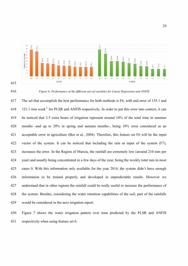
24
415
Figure 6: Performance of the different sets of variables for Linear Regression and ANFIS 416
The set that accomplish the best performance for both methods is F6, with and error of 155.1 and 417
121.1 min week-1 for PLSR and ANFIS respectively. In order to put this error into context, it can 418
be noticed that 2.5 extra hours of irrigation represent around 10% of the total time in summer 419
months -and up to 20% in spring and autumn months-, being 10% error considered as an 420
acceptable error in agriculture (Bos et al., 2004). Therefore, this feature set F6 will be the input 421
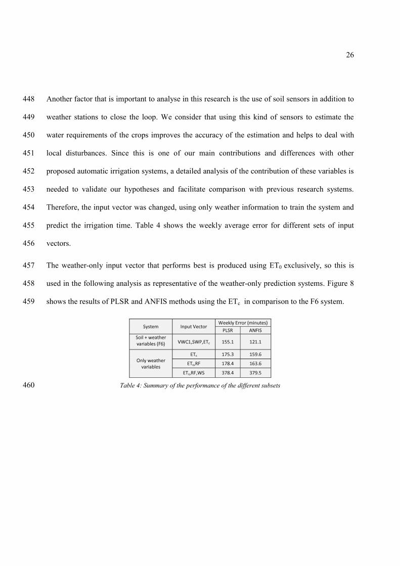
vector of the system. It can be noticed that including the rain as input of the system (F7), 422
increases the error. In the Region of Murcia, the rainfall are extremely low (around 210 mm per 423
year) and usually being concentrated in a few days of the year, being the weekly total rain in most 424
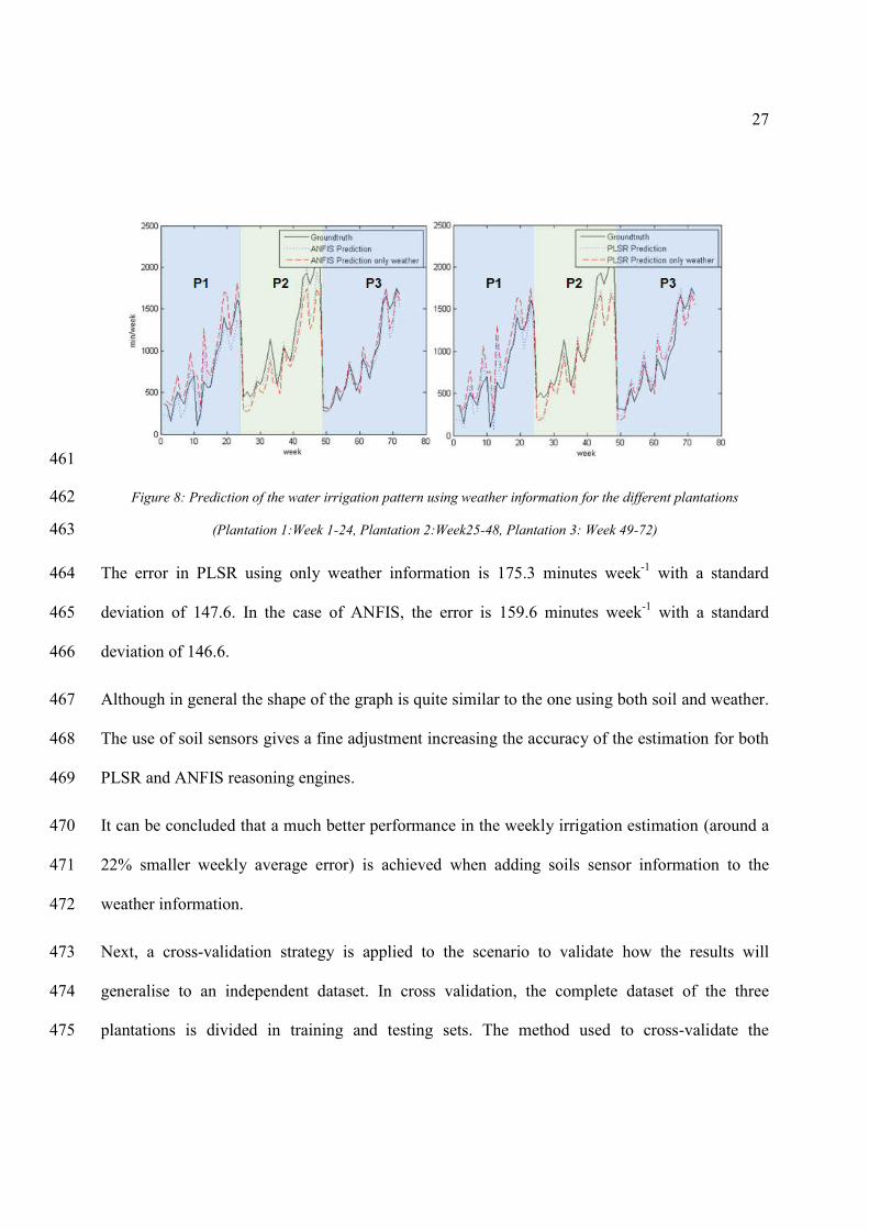
425
information to be trained properly and developed in unpredictable results. However we 426
understand that in other regions the rainfall could be really useful to increase the performance of 427
the system. Besides, considering the water retention capabilities of the soil, part of the rainfalls 428
would be considered in the next irrigation report. 429
Figure 7 shows the water irrigation pattern over time predicted by the PLSR and ANFIS 430
respectively when using feature set 6. 431
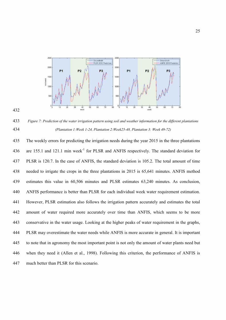
25
432
Figure 7: Prediction of the water irrigation pattern using soil and weather information for the different plantations 433
(Plantation 1:Week 1-24, Plantation 2:Week25-48, Plantation 3: Week 49-72) 434
The weekly errors for predicting the irrigation needs during the year 2015 in the three plantations 435
are 155.1 and 121.1 min week-1 for PLSR and ANFIS respectively. The standard deviation for 436
PLSR is 120.7. In the case of ANFIS, the standard deviation is 105.2. The total amount of time 437
needed to irrigate the crops in the three plantations in 2015 is 65,641 minutes. ANFIS method 438
estimates this value in 60,506 minutes and PLSR estimates 63,240 minutes. As conclusion, 439
ANFIS performance is better than PLSR for each individual week water requirement estimation. 440
However, PLSR estimation also follows the irrigation pattern accurately and estimates the total 441
amount of water required more accurately over time than ANFIS, which seems to be more 442
conservative in the water usage. Looking at the higher peaks of water requirement in the graphs, 443
PLSR may overestimate the water needs while ANFIS is more accurate in general. It is important 444
to note that in agronomy the most important point is not only the amount of water plants need but 445
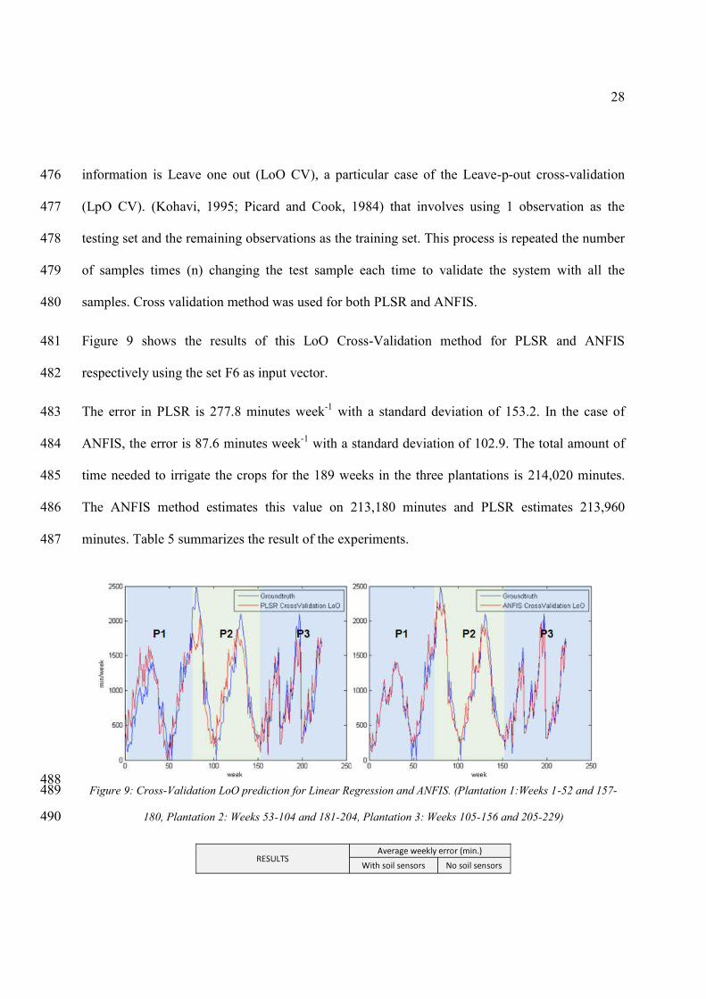
when they need it (Allen et al., 1998). Following this criterion, the performance of ANFIS is 446
much better than PLSR for this scenario. 447
26
Another factor that is important to analyse in this research is the use of soil sensors in addition to 448
weather stations to close the loop. We consider that using this kind of sensors to estimate the 449
water requirements of the crops improves the accuracy of the estimation and helps to deal with 450
local disturbances. Since this is one of our main contributions and differences with other 451
proposed automatic irrigation systems, a detailed analysis of the contribution of these variables is 452
needed to validate our hypotheses and facilitate comparison with previous research systems. 453
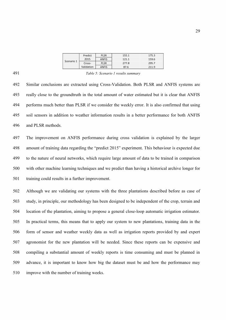
Therefore, the input vector was changed, using only weather information to train the system and 454
predict the irrigation time. Table 4 shows the weekly average error for different sets of input 455
vectors. 456
The weather-only input vector that performs best is produced using ET0 exclusively, so this is 457
used in the following analysis as representative of the weather-only prediction systems. Figure 8 458
shows the results of PLSR and ANFIS methods using the ETc in comparison to the F6 system. 459
Table 4: Summary of the performance of the different subsets 460
27
461
Figure 8: Prediction of the water irrigation pattern using weather information for the different plantations 462
(Plantation 1:Week 1-24, Plantation 2:Week25-48, Plantation 3: Week 49-72) 463
The error in PLSR using only weather information is 175.3 minutes week-1 with a standard 464
deviation of 147.6. In the case of ANFIS, the error is 159.6 minutes week-1 with a standard 465
deviation of 146.6. 466
Although in general the shape of the graph is quite similar to the one using both soil and weather. 467
The use of soil sensors gives a fine adjustment increasing the accuracy of the estimation for both 468
PLSR and ANFIS reasoning engines. 469
It can be concluded that a much better performance in the weekly irrigation estimation (around a 470
22% smaller weekly average error) is achieved when adding soils sensor information to the 471
weather information. 472
Next, a cross-validation strategy is applied to the scenario to validate how the results will 473
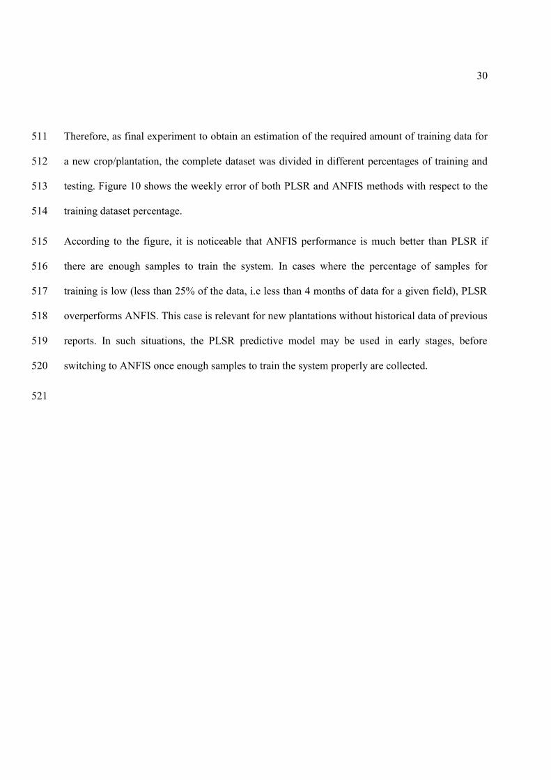
generalise to an independent dataset. In cross validation, the complete dataset of the three 474
plantations is divided in training and testing sets. The method used to cross-validate the 475
28
information is Leave one out (LoO CV), a particular case of the Leave-p-out cross-validation 476
(LpO CV). (Kohavi, 1995; Picard and Cook, 1984) that involves using 1 observation as the 477
testing set and the remaining observations as the training set. This process is repeated the number 478
of samples times (n) changing the test sample each time to validate the system with all the 479
samples. Cross validation method was used for both PLSR and ANFIS. 480
Figure 9 shows the results of this LoO Cross-Validation method for PLSR and ANFIS 481
respectively using the set F6 as input vector. 482
The error in PLSR is 277.8 minutes week-1 with a standard deviation of 153.2. In the case of 483
ANFIS, the error is 87.6 minutes week-1 with a standard deviation of 102.9. The total amount of 484
time needed to irrigate the crops for the 189 weeks in the three plantations is 214,020 minutes. 485
The ANFIS method estimates this value on 213,180 minutes and PLSR estimates 213,960 486
minutes. Table 5 summarizes the result of the experiments. 487
488 Figure 9: Cross-Validation LoO prediction for Linear Regression and ANFIS. (Plantation 1:Weeks 1-52 and 157-489
180, Plantation 2: Weeks 53-104 and 181-204, Plantation 3: Weeks 105-156 and 205-229) 490
29
Table 5: Scenario 1 results summary 491
Similar conclusions are extracted using Cross-Validation. Both PLSR and ANFIS systems are 492
really close to the groundtruth in the total amount of water estimated but it is clear that ANFIS 493
performs much better than PLSR if we consider the weekly error. It is also confirmed that using 494
soil sensors in addition to weather information results in a better performance for both ANFIS 495
and PLSR methods. 496
The improvement on ANFIS performance during cross validation is explained by the larger 497
498
to the nature of neural networks, which require large amount of data to be trained in comparison 499
with other machine learning techniques and we predict than having a historical archive longer for 500
training could results in a further improvement. 501
Although we are validating our systems with the three plantations described before as case of 502
study, in principle, our methodology has been designed to be independent of the crop, terrain and 503
location of the plantation, aiming to propose a general close-loop automatic irrigation estimator. 504
In practical terms, this means that to apply our system to new plantations, training data in the 505
form of sensor and weather weekly data as well as irrigation reports provided by and expert 506
agronomist for the new plantation will be needed. Since these reports can be expensive and 507
compiling a substantial amount of weekly reports is time consuming and must be planned in 508
advance, it is important to know how big the dataset must be and how the performance may 509
improve with the number of training weeks. 510
30
Therefore, as final experiment to obtain an estimation of the required amount of training data for 511
a new crop/plantation, the complete dataset was divided in different percentages of training and 512
testing. Figure 10 shows the weekly error of both PLSR and ANFIS methods with respect to the 513
training dataset percentage. 514
According to the figure, it is noticeable that ANFIS performance is much better than PLSR if 515
there are enough samples to train the system. In cases where the percentage of samples for 516
training is low (less than 25% of the data, i.e less than 4 months of data for a given field), PLSR 517
overperforms ANFIS. This case is relevant for new plantations without historical data of previous 518
reports. In such situations, the PLSR predictive model may be used in early stages, before 519
switching to ANFIS once enough samples to train the system properly are collected. 520
521
31
522
Figure 10: Performance comparison for Linear Regression and ANFIS with respect to the % of samples used to train 523
524
The goal is to predict the irrigation of a plantation based on its weather and soil measured 525
variables but using a SIDSS system trained exclusively with other fields. This will be the hardest 526
scenario as it will be necessary to predict the irrigation needs of a field with no previous irrigation 527
reports of that specific plantation. This scenario attempts to show the potential of our 528
methodology to create a universal irrigation estimator of a given crop -in our case, lemon trees- 529
for any given plantation, independently of the location and/or terrain. A lower performance can 530
be expected in comparison to what could be achieved by retraining the system with information 531
32
of the plantation (scenario 1), which is sacrificed for the benefit of not having to generate manual 532
irrigation report for new plantations. Cross validation, specifically leave-one_plantation-out is 533
applied in validation. Thus, 2014 and 2015 data from two of the plantations are used for training, 534
while the remaining plantation data (2014+2015) is used for testing. This is repeated 3 times, 535
leaving a different plantation out of the training set each time, and the results averaged. 536
Table 6 shows the error and standard deviation of this scenario for PLSR and ANFIS using 537
different features vector used to compare the performance. 538
Table 6: Scenario 2 results summary 539
The best feature vector F6 used in scenario 1 is used as input. In this case PLSR outperforms 540
ANFIS with an average error of 257.0 minutes in comparison with 323.3 minutes for ANFIS. 541
However, we noticed that, in this scenario, removing the VWC1 sensor results in a better 542
performance for both methods as a universal estimator. This is explained because the VWC 543
sensor is very dependent on the soil where it is installed and, as both algorithms were trained with 544
a sensor installed in a different plantation than the one that is predicting, the provided information 545
introduces noise and does not help the system to estimate properly the water need. This does not 546
33
happen, however, with the SWP sensor, which quantifies the tendency of water to move from one 547
area to another in the soil and it is less dependent on the soil installed. Removing the VWC 548
sensor results in a better performance of the system obtaining an average weekly error of 194.4 549
minutes with PLSR and 197.4 minutes with ANFIS. This result proves that there is certain 550
potential to develop a universal estimator using our system for a given crop, although this means 551
an increase of the average error. This error could be reduced if more than 2 plantations of the 552
same crop were available for training. Both PLSR and ANFIS performs similarly, being PLSR 553
slightly better. 554
555
This paper describes the design and development of an automatic decision support system to 556
manage irrigation in agriculture. The main characteristic of system is the use of continuous soil 557
measurements to complement climatic parameters to precisely predict the irrigation needs the 558
crops, in contrast with previous works that are based only on weather variables 559
the quantity of water required by the crops. The use of real-time information from the soil 560
parameters in a closed loop control scheme allows adapting the decision support system to local 561
perturbations, avoiding the accumulative effect due to errors in consecutive weekly estimation, 562
and/or detecting if the irrigation calculated for the SIDSS has been performed by the farmer. The 563
analysis of the performance of the system is accomplished comparing the decisions taken by a 564
human expert and the decision support component. Two machine learning techniques, PLSR and 565
ANFIS, have been proposed as the basis of our reasoning engine and analysed in order to obtain 566
the best performance. 567
34
The experiments have taken place in three commercial plantations of citrus trees located in the 568
South-East of Spain. A first experimental scenario shows a comparison of the system´s 569
performance using soil sensors in addition to the weather information for predicting year 2015 570
using 2014 information to train the system. The usage of soil sensor in the three plantations 571
accomplished a 22% less of weekly error in comparison to the performance of using only weather 572
information. 573
A second scenario shows the potential of our system as universal estimator for a given crop, i.e 574
the use case of installing the system in a new plantation, not having previous information of it. 575
For this application, VWC sensors should be removed due to their high dependence with the soil 576
type. Although, as expected, the estimation error increases in this scenario, it does not require 577
historical data from agronomical reports to be retrained, which implies a significant advantage, in 578
particular for new plantations in early stages. If more training data from a bigger variety of field 579
were available, a better performance in this scenario could be expected. Another possible 580
improvement for this scenario will be the addition of a VWC to get a better performance than 581
using only the matric potential sensors. However, in order to use the VWC sensor in this 582
scenario, a precise study of the soil textures of the plantation will be required to extrapolate the 583
VWC sensor information to similar soil textures where the DSS was trained. 584
For future research, we aim to extend and evaluate the system in plantations different than citrus 585
and analyse the performance under several conditions and regions. Thus, adding the weather 586
forecast as input of the SIDSS could help to improve the next week irrigation schedule and 587
consider the predicted rainfall in our estimation. Similarly, past rainfall information, that did not 588
prove beneficial in our system due to the region of Murcia characteristics, may become a good 589
35
factor to improve the accuracy of the system in regions with a more regular and predictable 590
raining pattern. We also aim to capture a bigger dataset that will allow us to generate more 591
general models towards a universal irrigation estimator of a given crop. This dataset will also 592
explore the use of multiple sensors per plantation in order to address inhomogeneous ground 593
conditions in the different plantation as well as provide more input information to the system for 594
a better reasoning. 595
596
The development of this work was supported by the Spanish Ministry of Science and Innovation 597
through the projects MICINN, AGL2010-19201-C04-04 and MINECO, AGL2013-49047-C2-1-598
R. We would like to thank Widhoc Smart Solutions S.L. for 599
letting us use their facilities and equipment to carry out the tests. 600
601
602
Abrisqueta, I., Conejero, W., Valdés-Vela, M., Vera, J., Ortuño, M.F., Ruiz-Sánchez, M.C., 2015. 603
Stem water potential estimation of drip-irrigated early-maturing peach trees under Mediterranean 604
conditions. Computers and Electronics in Agriculture 114, 7 13. 605
doi:10.1016/j.compag.2015.03.004 606
Adeloye, A.J., Rustum, R., Kariyama, I.D., 2012. Neural computing modeling of the reference 607
crop evapotranspiration. Environ. Model. Softw. 29, 61 73. doi:10.1016/j.envsoft.2011.10.012 608
Allen, R.G., Pereira, L.S., Raes, D., Smith, M., 1998. Crop Evapotranspiration: Guidelines for 609
36
Computing Crop Water Requirements. FAO Irrigation and Drainage Paper No. 56. 610
Belousov, A.I., Verzakov, S.A., von Frese, J., 2002. A flexible classification approach with 611
optimal generalisation performance: support vector machines. Chemom. Intell. Lab. Syst. 64, 15612
25. doi:10.1016/S0169-7439(02)00046-1 613
Bos, M.G., Burton, M.A., Molden, D.J. (Eds.), 2004. Irrigation and drainage performance 614
assessment: practical guidelines. CABI, Wallingford. 615
Campos, I., Balbontín, C., González-Piqueras, J., González-Dugo, M.P., Neale, C.M.U., Calera, 616
A., 2016. Combining a water balance model with evapotranspiration measurements to estimate 617
total available soil water in irrigated and rainfed vineyards. Agricultural Water Management 165, 618
141 152. doi:http://dx.doi.org/10.1016/j.agwat.2015.11.018 619
Cardenas-Lailhacar, B., Dukes, M.D., 2010. Precision of soil moisture sensor irrigation 620
controllers under field conditions. Agric. Water Manag. 97, 666 672. 621
doi:10.1016/j.agwat.2009.12.009 622
623
environmental knowledge system for sustainable agricultural decision support. Environ. Model. 624
Softw. 52, 264 272. doi:10.1016/j.envsoft.2013.10.004 625
Fisher, R.A., 1938. The Statistical Utilization of Multiple Measurements. Ann. Eugen. 8, 376626
386. doi:10.1111/j.1469-1809.1938.tb02189.x 627
Giusti, E., Marsili-Libelli, S., 2015. A Fuzzy Decision Support System for irrigation and water 628
conservation in agriculture. Environ. Model. Softw. 63, 73 86. 629
doi:10.1016/j.envsoft.2014.09.020 630
37
Guariso, G., Rinaldi, S., Soncini-Sessa, R., 1985. Decision support systems for water 631
management: The Lake Como case study. Eur. J. Oper. Res. 21, 295 306. doi:10.1016/0377-632
2217(85)90150-X 633
IDAE, 2005. Ahorro y Eficiencia Energética en Agricultura de Regadío. Madrid. 634
Jang, J.-S.R., 1993. ANFIS: adaptive-network-based fuzzy inference system. IEEE Trans. Syst. 635
Man Cybern. 23, 665 685. doi:10.1109/21.256541 636
Jensen, M.E., Robb, D.C.N., Franzoy, C.E., 1970. Scheduling Irrigations Using Climate-Crop-637
Soil Data. J. Irrig. Drain. Div. 96, 25 38. 638
Jones, H.G., 2004. Irrigation scheduling: advantages and pitfalls of plant-based methods. J. Exp. 639
Bot. 55, 2427 2436. doi:10.1093/jxb/erh213 640
King, B.A., Shellie, K.C., 2016. Evaluation of neural network modeling to predict non-water-641
stressed leaf temperature in wine grape for calculation of crop water stress index. Agricultural 642
Water Management 167, 38 52. doi:http://dx.doi.org/10.1016/j.agwat.2015.12.009 643
Kohavi, R., 1995. A Study of Cross-validation and Bootstrap for Accuracy Estimation and Model 644
Selection, in: Proceedings of the 14th International Joint Conference on Artificial Intelligence - 645
ncisco, CA, USA, pp. 1137646
1143. 647
Kramer, P.J., Boyer, J.S., 1995. Water relations of plants and soils. Academic Press, Inc. 648
38
López Riquelme, J.A., Soto, F., Suardíaz, J., Sánchez, P., Iborra, A., Vera, J.A., 2009. Wireless 649
Sensor Networks for precision horticulture in Southern Spain. Computers and Electronics in 650
Agriculture 68, 25 35. doi:10.1016/j.compag.2009.04.006 651
Maton, L., Leenhardt, D., Goulard, M., Bergez, J.-E., 2005. Assessing the irrigation strategies 652
over a wide geographical area from structural data about farming systems. Agric. Syst. 86, 293653
311. doi:10.1016/j.agsy.2004.09.010 654
Naor, A., Hupert, H., Greenblat, Y., Peres, M., Kaufman, A., Klein, I., 2001. The Response of 655
Nectarine Fruit Size and Midday Stem Water Potential to Irrigation Level in Stage III and Crop 656
Load. J. Am. Soc. Hortic. Sci. 126, 140 143. 657
Navarro-Hellín, H., Torres-Sánchez, R., Soto-Valles, F., Albaladejo-Pérez, C., López-Riquelme, 658
J.A., Domingo-Miguel, R., 2015. A wireless sensors architecture for efficient irrigation water 659
management. Agric. Water Manag., New proposals in the automation and remote control of water 660
management in agriculture: agromotic systems 151, 64 74. doi:10.1016/j.agwat.2014.10.022 661
Picard, R.R., Cook, R.D., 1984. Cross-Validation of Regression Models. Journal of the American 662
Statistical Association 79, 575 583. doi:10.2307/2288403 663
Puerto, P., Domingo, R., Torres, R., Pérez-Pastor, A., García-Riquelme, M., 2013. Remote 664
management of deficit irrigation in almond trees based on maximum daily trunk shrinkage. Water 665
relations and yield. Agric. Water Manag. 126, 33 45. doi:10.1016/j.agwat.2013.04.013 666
SIAM, 2015. Red del Sistema de Información Agrario de Murcia. URL siam.imida.es 667
Smith, M., 2000. The application of climatic data for planning and management of sustainable 668
rainfed and irrigated crop production. Agric. For. Meteorol. 103, 99 108. doi:10.1016/S0168-669

39
1923(00)00121-0 670
Soulis, K.X., Elmaloglou, S., Dercas, N., 2015. Investigating the effects of soil moisture sensors 671
positioning and accuracy on soil moisture based drip irrigation scheduling systems. Agric. Water 672
Manag. 148, 258 268. doi:10.1016/j.agwat.2014.10.015 673
Sreekanth, M.S., Rajesh, R., Satheeshku, J., 2015. Extreme Learning Machine for the 674
Classification of Rainfall and Thunderstorm. Journal of Applied Sciences 15, 153 156. 675
doi:10.3923/jas.2015.153.156 676
Valdés-Vela, M., Abrisqueta, I., Conejero, W., Vera, J., Ruiz-Sánchez, M.C., 2015. Soft 677
computing applied to stem water potential estimation: A fuzzy rule based approach. Comput. 678
Electron. Agric. 115, 150 160. doi:10.1016/j.compag.2015.05.019 679
Wang, Z., Palade, V., Xu, Y., 2006. Neuro-Fuzzy Ensemble Approach for Microarray Cancer 680
Gene Expression Data Analysis, in: 2006 International Symposium on Evolving Fuzzy Systems. 681
Presented at the 2006 International Symposium on Evolving Fuzzy Systems, pp. 241 246. 682
doi:10.1109/ISEFS.2006.251144 683
Wold, S., Ruhe, A., Wold, H., Dunn, I., W., 1984. The Collinearity Problem in Linear 684
Regression. The Partial Least Squares (PLS) Approach to Generalized Inverses. SIAM J. Sci. 685
Stat. Comput. 5, 735 743. doi:10.1137/0905052 686
Wold, S., Sjöström, M., Eriksson, L., 2001. PLS-regression: a basic tool of chemometrics. 687
Chemom. Intell. Lab. Syst., PLS Methods 58, 109 130. doi:10.1016/S0169-7439(01)00155-1 688
Zadeh, L.A., Klir, G.J., Yuan, B., 1996. Fuzzy Sets, Fuzzy Logic, and Fuzzy Systems: Selected 689
Papers by Lotfi A Zadeh, Advances in Fuzzy Systems Applications and Theory. WORLD 690

40
SCIENTIFIC. 691
Zwart, S.J., Bastiaanssen, W.G.M., 2004. Review of measured crop water productivity values for 692
irrigated wheat, rice, cotton and maize. Agric. Water Manag. 69, 115 133. 693
doi:10.1016/j.agwat.2004.04.007 694