NTIA Report 97-340

A Digital Simulation Model for Local Multipoint and Multichannel Multipoint

Distribution Services

Roger A. Dalke

George A. Hufford Ronald L. Ketchum

U.S. DEPARTMENT OF COMMERCE William M. Daley, Secretary

Larry Irving, Assistant Secretary

for Communications and Information

July 1997

iii

PRODUCT DISCLAIMER

Certain commercial companies, equipment, instruments, and materials are identified in this report to specify adequately the technical aspects of the reported results. In no case does such identification imply recommendation or endorsement by the National Telecommunications and Information Administration, nor does it imply that the material or equipment identified is necessarily the best available for the purpose.

v

CONTENTS PRODUCT DISCLAIMER ........................................................................................................... iii ABSTRACT.....................................................................................................................................1 1. INTRODUCTION .....................................................................................................................1 2. COMPUTER SIMULATION MODEL.....................................................................................2 2.1 RF Signal .............................................................................................................................3 2.1.1 Number of RF Signals ................................................................................................4 2.1.2 RF Bandwidth, Spectral Guard, and Rolloff...............................................................4 2.2 Transmitter Amplifier ..........................................................................................................6 2.2.1 Traveling Wave Tube Amplifier.................................................................................6 2.3 Channel ................................................................................................................................7 2.3.1 Propagation Channel Models......................................................................................8 2.3.2 Equalizer ...................................................................................................................11 2.4 Inner Loop..........................................................................................................................11 2.5 Outer Loop.........................................................................................................................12 3. APPLICATIONS .....................................................................................................................13 3.1 The Additive White Gaussian Noise Channel ...................................................................13 3.2 Nonlinear Amplifier...........................................................................................................13 3.3 The Propagation Channel...................................................................................................15 4. SUMMARY.............................................................................................................................19 5. REFERENCES ........................................................................................................................20 APPENDIX A: SIMULATION MODEL USER’S GUIDE .........................................................23

A DIGITAL SIMULATION MODEL FOR LOCAL MULTIPOINT AND MULTICHANNEL MULTIPOINT DISTRIBUTION SERVICES

Roger Dalke, George Hufford, and Ronald Ketchum∗

The Institute for Telecommunication Sciences has developed a computer simulation model that can be used to predict coverage and quality of service for proposed terrestrial communication systems that broadcast digital television such as local multipoint distribution services and multichannel multipoint distribution services. The model includes a variety of digital modulation schemes that have been proposed for these services. The model also contains a nonlinear amplifier that allows the user to evaluate the effects of intermodulation distortion on performance. In addition to a simple additive white Gaussian noise channel, three different propagation channels are included: a simple two-ray channel; and two more complex channels based on measurements of broadband signals in various geographic environments. A description of the simulation model as well as examples of applications are given in this report.

Key words: local multipoint distribution services (LMDS); multichannel multipoint distribution

services (MMDS); digital broadcast services; propagation channel model; nonlinear amplifier; traveling wave tube amplifier (TWTA); digital communication systems; simulation

1. INTRODUCTION An important consideration in the design and implementation of local multipoint distribution services (LMDS) and multichannel multipoint distribution services (MMDS) for digital broadcast television is the prediction of coverage area and quality of service. Such a terrestrial broadcast system will have a nonlinear, band-limited, channel subject to additive and multiplicative noise. It is important that the system designer have a basis for determining equipment specifications that will provide the lowest probability of bit errors and hence maximize the coverage area and quality of service. Such specifications include amplifier backoff, transmitter and receiver filter rolloff, methods used to mitigate multiplicative noise (e.g., equalizer parameters), and error detection/correction coding. Since it is difficult, if not impossible, to make theoretical predictions for such a system, computer simulation models are necessary to estimate the adequacy of system specifications. In this report, we describe simulation software that has been developed for the analysis of terrestrial broadcast of digital television. Through its user interface, the model allows the user to vary parameters such as RF signal specifications (e.g., digital modulations schemes, and symbol rates/bandwidth), transmitter amplifier, and propagation channel models (including equalization).

∗ The authors are with the Institute for Telecommunication Sciences, National Telecommunications and Information Administration, U.S. Department of Commerce, Boulder, CO 80303.

2

Section 2 describes the theoretical basis for the model and the various options available through the user interface. The primary purpose of such a model is to predict symbol error probabilities based on the operational environment of the system. In Section 3, we provide applications of the simulation model which include the influence of a nonlinear amplifier and noise (additive and multiplicative) on the reception of transmitted symbols. Of particular interest are the interplay between the RF signal and the physical environment where the terrain and propagation path geometry have a significant influence. The simulation model allows for the selection of propagation channel models that have been developed based on radio propagation measurements. Measured data from an environment similar to the proposed MMDS in the Los Angeles, California area were used to estimate propagation channel model parameters. Using these parameters, bit and symbol error probabilities as a function of signal-to-noise ratio (SNR) are presented. Once the required SNR has been estimated, it is necessary to determine if the proposed system will provide the level of service required. Propagation models that include the system geometry, terrain, transmitter/receiver characteristics, antenna characteristics, and path attenuation can be used to estimate the availability of the desired SNR in the proposed service area. Such estimates can be made using the Telecommunications Analysis Services (TA Services) Communication System Performance Model (CSPM). TA Services is an ITS facility that provides industry and Government agencies access to the latest ITS computer programs and associated databases in the form of easy-to-use time-sharing computer programs on a cost-reimbursable basis. The computer simulation model was designed for use on a personal computer and has a graphical user interface (GUI). A user’s guide for this interface is provided in Appendix A.

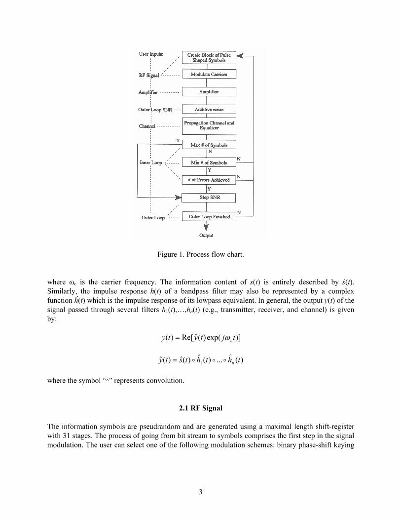
2. COMPUTER SIMULATION MODEL In this section, we describe the computer simulation model developed for the analysis of a nonlinear band-limited channel and serial transmission of symbols. This model is applicable to the analysis of both LMDS and MMDS. The process flow for the model is shown in Figure 1 and a detailed description of each module is given below. The simulation program is written in Fortran and has a GUI that is described in Appendix A (User’s Guide). The following sections provide a description of how the options available to the user are implemented. In general, the computer simulation of a bandpass channel is performed at baseband using complex-valued functions of time. This is essential for SHF and EHF bands where theoretical limitations imposed by the Sampling Theorem [1] preclude simulation of the modulated carrier. . Baseband analysis is accomplished by representing the signal s(t) by a complex function ŝ(t):

[ ]tjtsts cωexp()(ˆRe)( =

3

Figure 1. Process flow chart. where ωc is the carrier frequency. The information content of s(t) is entirely described by ŝ(t). Similarly, the impulse response h(t) of a bandpass filter may also be represented by a complex function ĥ(t) which is the impulse response of its lowpass equivalent. In general, the output y(t) of the signal passed through several filters h1(t),…,hn(t) (e.g., transmitter, receiver, and channel) is given by:

)]exp()(ˆRe[)( tjtyty cω=

)(ˆ...)(ˆ)(ˆ)(ˆ 1 ththtsty nooo= where the symbol “◦” represents convolution.

2.1 RF Signal The information symbols are pseudrandom and are generated using a maximal length shift-register with 31 stages. The process of going from bit stream to symbols comprises the first step in the signal modulation. The user can select one of the following modulation schemes: binary phase-shift keying

4

(BPSK); quaternary phase-shift keying (QPSK); 16 quadrature amplitude modulation (16QAM); and 64QAM. The constellation of 64 symbols can be implemented as either 64QAM or 64TCM (trellis-coded modulation). The main advantage of trellis coding is the achievement of significant coding gains over uncoded multilevel modulation, however, at the expense of information bit(s). The particular version of TCM implemented in the model is the simplest of the suggestions given by [2]. It uses the 6-bit constellation specified by [3] where one of the bits is reserved for parity. The encoder has eight states and the decoder uses the Viterbi algorithm [4]. The coding gain relative to 5-bit uncoded modulation (32QAM) is 3.77 dB. The bit error ratio for both 64QAM and 64TCM computed by the model for an ideal channel (no multipath) are shown in Section 3. It should be noted that the TCM implementation is designed to provide an estimate of the level of improvement that may be achieved in the presence of a nonlinear transmitter and propagation channel with multiplicative noise. This model is not intended to be used to determine the optimum coding scheme or implementation. 2.1.1 Number of RF Signals Consideration of the effects of interference and distortion due to the use of a nonlinear amplifier (e.g., traveling wave tube amplifier; TWTA) is of particular importance in an environment containing several adjacent RF signals that can produce intermodulation interference. The user can select up to seven adjacent RF signals (multiple carriers) to be implemented. This feature is most useful for LMDS where the use of nonlinear amplifiers is a distinct possibility. The user may select any one of the seven RF signals for decoding, hence intermodulation effects on the center and end RF signals can be evaluated. 2.1.2 RF Bandwidth, Spectral Guard, and Rolloff The remaining RF signal options are: RF bandwidth, spectral guard, and transmitter filter rolloff. There are many different definitions of bandwidth (e.g., absolute, 3-dB, equivalent, and power bandwidth). In this model, bandwidth refers to the spacing between multiple RF signals (carriers). For the purposes of the model, this is a practical definition since the filters are implemented as finite impulse response (FIR) filters. The spectral guard option allows the user to increase the overall bandwidth by a specified amount stated as a percentage. The guard provides additional separation of the adjacent RF signals. An ideal pulse-shaping modulation scheme designed to minimize transmitter/receiver filter induced intersymbol interference (ISI) is used in this model. The transmitter filter is a raised cosine pulse shape that satisfies Nyquist’s first criterion [5]. The user may specify a rolloff of 10-100%. The RF bandwidth, symbol rate, and the rolloff are related as follows:

5

⎟⎠⎞

⎜⎝⎛ +⎟⎠⎞

⎜⎝⎛ +

=

100%1

100%1 guardrolloff

bandwidthrfratesymbol .

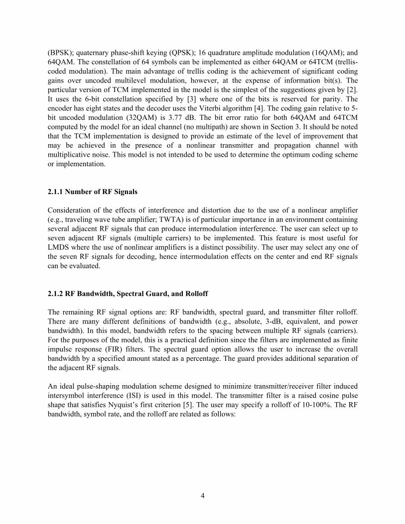
In this model, the specifications for the receiver filter and the transmitter filter are directly linked. The receiver filter is implemented as an FIR filter and utilizes a Hamming [1] window. The rolloff of the receiver filter is steeper than the transmitter filter. The filter transition width is bounded (in frequency) by the reciprocal of the symbol rate and the upper limit of the RF bandwidth. The normalized frequency response of the transmitter and corresponding receiver filter for a 6-MHz bandwidth and 50% rolloff is shown in Figure 2. It should be noted that while the convolution of the transmitter and receiver filter is roughly equal to the transmitter filter response, there is some deviation from the ideal Nyquist criterion, resulting in a small amount of ISI. By design, increasing the guard band moves the upper and lower limits of the receiver filter transition band so that ISI is decreased. While in principle, for a linear system, it is possible to completely eliminate ISI due to these filters, a nonlinear amplifier distorts the response of the transmitter filter. In this case, elimination of ISI due to pulse shaping is no longer possible. Furthermore, in the nonlinear case, the rolloff factor becomes important since ringing due to small rolloff factors is more severely distorted by the nonlinear amplifier.

Figure 2. Transmitter and receiver filter spectrum showing rolloff and guard.

6

2.2 Transmitter Amplifier The model provides for the selection of either a linear or nonlinear (TWTA) amplifier. The nonlinear amplifier applies the amplitude and phase characteristics described below to the modulated RF signals. When several carriers (RF signals) are present, the nonlinear amplifier will introduce intermodulation interference resulting in the suppression of signals and disproportionate power sharing. For a single carrier, amplitude modulation will result in unwanted phase modulation of the signal. For purely phase-modulated signals, the amplitude-to-phase conversion will result in a rotated symbol constellation and is readily corrected (e.g., by an equalizer). 2.2.1 Traveling Wave Tube Amplifier The baseband equivalent of a memoryless nonlinear TWTA can be obtained by writing s(t) as:

))(cos()()( tttAts c θω +=

⎟⎟⎠

⎞⎜⎜⎝

⎛=+= −

)()(

tan)()()()( 122

tsts

ttststAi

qqi θ

))(sin()()())(cos()()( ttAtsttAts qi θθ == .

The TWTA is then represented by two nonlinear functions G and F which describe amplitude and phase nonlinearity, respectively [6]:

)]exp()(ˆRe[)( tjtztz cω=

)])([)(cos()]([)](ˆRe[ tAFttAGtz += θ

)])([)(sin()]([)](ˆIm[ tAFttAGtz += θ .

The baseband representation of the output of the nonlinear amplifier is given by )(ˆ tz . The nonlinear functions G and F are typically represented by two-parameter models as:

21

1

1][

AA

AGβα+

=

22

22

1][

AAAF

βα+

= .

7

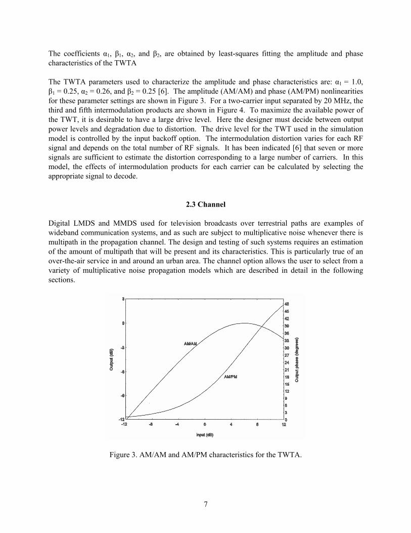
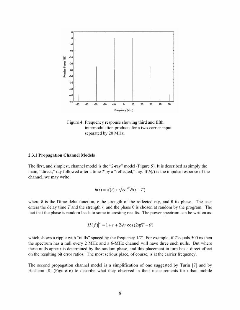
The coefficients α1, β1, α2, and β2, are obtained by least-squares fitting the amplitude and phase characteristics of the TWTA The TWTA parameters used to characterize the amplitude and phase characteristics are: α1 = 1.0, β1 = 0.25, α2 = 0.26, and β2 = 0.25 [6]. The amplitude (AM/AM) and phase (AM/PM) nonlinearities for these parameter settings are shown in Figure 3. For a two-carrier input separated by 20 MHz, the third and fifth intermodulation products are shown in Figure 4. To maximize the available power of the TWT, it is desirable to have a large drive level. Here the designer must decide between output power levels and degradation due to distortion. The drive level for the TWT used in the simulation model is controlled by the input backoff option. The intermodulation distortion varies for each RF signal and depends on the total number of RF signals. It has been indicated [6] that seven or more signals are sufficient to estimate the distortion corresponding to a large number of carriers. In this model, the effects of intermodulation products for each carrier can be calculated by selecting the appropriate signal to decode.

2.3 Channel Digital LMDS and MMDS used for television broadcasts over terrestrial paths are examples of wideband communication systems, and as such are subject to multiplicative noise whenever there is multipath in the propagation channel. The design and testing of such systems requires an estimation of the amount of multipath that will be present and its characteristics. This is particularly true of an over-the-air service in and around an urban area. The channel option allows the user to select from a variety of multiplicative noise propagation models which are described in detail in the following sections.

Figure 3. AM/AM and AM/PM characteristics for the TWTA.

8

Figure 4. Frequency response showing third and fifth intermodulation products for a two-carrier input separated by 20 MHz.

2.3.1 Propagation Channel Models The first, and simplest, channel model is the “2-ray” model (Figure 5). It is described as simply the main, “direct,” ray followed after a time T by a “reflected,” ray. If h(t) is the impulse response of the channel, we may write

)()()( Ttretth j −+= δδ θ where δ is the Dirac delta function, r the strength of the reflected ray, and θ its phase. The user enters the delay time T and the strength r, and the phase θ is chosen at random by the program. The fact that the phase is random leads to some interesting results. The power spectrum can be written as

)2(cos21)( 2 θπ −++= fTrrfH which shows a ripple with “nulls” spaced by the frequency 1/T. For example, if T equals 500 ns then the spectrum has a null every 2 MHz and a 6-MHz channel will have three such nulls. But where these nulls appear is determined by the random phase, and this placement in turn has a direct effect on the resulting bit error ratios. The most serious place, of course, is at the carrier frequency. The second propagation channel model is a simplification of one suggested by Turin [7] and by Hashemi [8] (Figure 6) to describe what they observed in their measurements for urban mobile

9

communications. The program calls it the “Turin/Hashemi” model and it is described by the equation

∑=

−−−+=n

kk

jk

k texTT

rtth k

1

)()22

1exp()()( τδτ

λδ θ

where r is the strength in the tail of reflections; the delay times τk form a Poisson sequence with average rate λ; T measures the delay spread and is the decay time of the tail; the xk are normally distributed with mean 0, standard deviation σ, and a nonzero correlation amongst themselves, and the θk are independent uniformly distributed random phases. At present, r and T are user-supplied while λ = 3 arrivals per µs, σ = 5.5 dB, n=6, and the xk and θk are chosen by the program. The third, and probably most realistic [9], model is called the WSSUS (wide sense stationary uncorrelated scatterers) model (Figure 7). Like the second model, it consists of a direct ray followed by an exponentially decaying tail of delayed rays. Now, however, there are a very large number, all of them pairwise independent. The channel can be expressed as:

∑∞

=

−−+=

1

2 )()()(k

kT

k

ktzeTrtth τδτδ

τ

where again r is the strength of the tail and T is the decay time serving to measure the delay spread, and where now the zk are independent complex random numbers normally distributed with uniformly distributed phases. In principle, the sampling time τ is supposed to tend to zero but for practical use we assume that it equals the sampling time for the signal ŝ(t) (which is usually a small fraction of the symbol length).

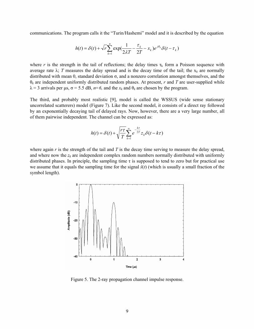
Figure 5. The 2-ray propagation channel impulse response.

10

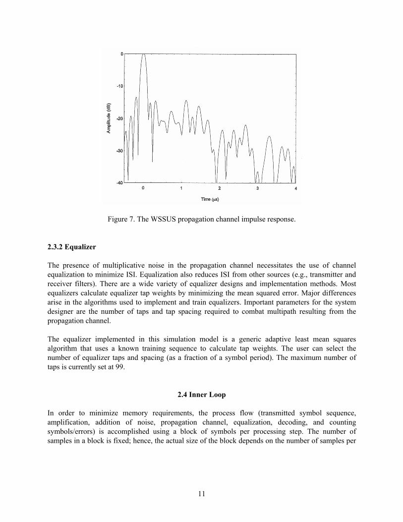
Figure 6. The Turin/Hashemi propagation channel impulse response. In Figures 5, 6, and 7 we have used an option of the simulation program to provide example plots of these three propagation channel models after they have passed through the simulated receiver filter. In all three cases we have chosen the parameters T = 1 µs and r = 0.1 (R = –10 dB). The resulting plots show the so-called “power delay profiles” of the generated impulse responses in decibels relative to the direct ray. All three models require user input for the “delay spread” T and the strength r (or, represented in decibels, R) of the tail of delayed rays. The choice will, of course, depend on the purpose of the study and an analysis of measurements that are appropriate for the area under study. Unfortunately, we do not know of measurements that might correspond to, say, MMDS operations. Wepman [10] reported on measurements at nearly 2 GHz, but these simulated the personal communications services (PCS) environment and used fairly low antenna heights. The PCS data yields typical propagation parameters of T = 200 ns and R = –5 dB. We also noted more extreme values of 1 µs delay and 0 dB in strength. On the other hand, Hufford [9] described measurements using high television transmitters looking down on a city, just as one would suppose an MMDS installation would be situated. Although the measurements were at about 600 MHz, they probably represent the best approximation of an MMDS situation. The results found typical values of T = 1 µs and R = –10. In the extreme, values of R as large as –3 dB were also noted. Interestingly, when a directive antenna was used, the typical values changed to T = 4 µs and R = –14 dB. Evidently, although the strength decreases, the delayed rays arrive for quite a while. To simulate a realistic case, we would suggest the WSSUS model using the typical values of T = 3 µs, R = –10 dB, or, for a directive antenna, T = 2 µs, R = –14 dB. In any case, one seems to obtain in the end an ISI noise (without equalization and with no thermal noise) equal to about the value of R. The value of T seems to have only a secondary influence, although it certainly becomes important in the design of an equalizer.

11

Figure 7. The WSSUS propagation channel impulse response. 2.3.2 Equalizer The presence of multiplicative noise in the propagation channel necessitates the use of channel equalization to minimize ISI. Equalization also reduces ISI from other sources (e.g., transmitter and receiver filters). There are a wide variety of equalizer designs and implementation methods. Most equalizers calculate equalizer tap weights by minimizing the mean squared error. Major differences arise in the algorithms used to implement and train equalizers. Important parameters for the system designer are the number of taps and tap spacing required to combat multipath resulting from the propagation channel. The equalizer implemented in this simulation model is a generic adaptive least mean squares algorithm that uses a known training sequence to calculate tap weights. The user can select the number of equalizer taps and spacing (as a fraction of a symbol period). The maximum number of taps is currently set at 99.

2.4 Inner Loop In order to minimize memory requirements, the process flow (transmitted symbol sequence, amplification, addition of noise, propagation channel, equalization, decoding, and counting symbols/errors) is accomplished using a block of symbols per processing step. The number of samples in a block is fixed; hence, the actual size of the block depends on the number of samples per

12

symbol. This quantity is variable based on the number of RF signals and is set to ensure a sufficient number of samples for the highest frequency of interest. Typically about 500-1000 symbols are in a block. The complete processing of a block of symbols comprises an iteration of the inner loop. The inner loop parameters allow the user to specify the number of iterations required to yield an adequate estimate of the symbol error ratio (SER) for a given SNR, multipath propagation channel, or level of intermodulation interference. The number of inner loop iterations is controlled by the user-supplied parameters: minimum number of symbols, number of errors, and absolute maximum number of symbols. SER’s are calculated by letting the number of iterations continue until the error count reaches a predetermined number. If this number is n, if the errors appear independently of the others, and if the SER is small, the SER is estimated as n divided by the total number of symbols. In this case, the estimation will have a relative error whose root mean square is approximately 1/ n . Hence, for n as small as 10, the results would give at least the right order of magnitude. The size of n is important since it has a significant effect on the processing time. The inner loop processes blocks of symbols until the user-supplied error limit is attained or exceeded. For small SER’s, the bit error ratio (BER) can be estimated by assuming that a symbol error is due to a single wrong bit. This is a reasonable approach since large SER’s are usually not of interest as well as being of somewhat dubious accuracy. The minimum number of symbols option is useful when the number of errors will be exceeded quickly and it is desirable to process a sufficient number of symbols to achieve reasonable results. The inner loop iterations will continue until the specified minimum number of symbols has been received. It is often desirable to set an absolute limit on the number of symbols required to complete the inner loop calculations. The ability to specify the absolute maximum number of symbols is provided in the inner loop. This will override the number of errors and advance to the next iteration of the outer loop. This feature can be useful in preventing excessively long calculations. When the number of errors or the absolute limit on the number of symbols has been reached (assuming the number of symbols exceeds the specified minimum), the program advances to the outer loop.

2.5 Outer Loop As shown in Figure 1, the inner loop is nested within the outer loop. The outer loop allows the user to perform calculations over a range of SNR’s and/or rea1izations of propagation channel models. User inputs include a starting SNR, increment, and number of iterations. These options are used primarily to specify the desired range of SNR’s.

13

By design, the propagation channel models described in Section 2.3 are random processes with the user suppling the two parameters, strength and delay (which correspond to what is often loosely referred to as delay spread). By performing several iterations using the outer loop, the model can be used to predict time and location variability. Location variability refers to changes in fading characteristics, due for example to variations in phase of the multipath at different locations, and time variability refers to changes in fading characteristics at a given location due to changes in atmospheric conditions. Thus, by iterating over the outer loop for a fixed SNR, variability in the propagation channel can be estimated. In the case of the WSSUS channel model, each scatterer is given a random amplitude (Rayleigh distributed) and phase (uniformly distributed). New random numbers are used for each iteration of the outer loop. Only the phase is varied in the 2-ray model. In all cases, the channel filter is constrained by the user-specified delay and strength.

3. APPLICATIONS As indicated in the previous section, the model allows for the selection of modulation schemes, amplifiers (linear, nonlinear), propagation channel models, and noise levels. In this section, we provide examples of calculations that illustrate the capabilities of the simulation model and are applicable to the design of MMDS/LMDS. In particular, we have made calculations using a statistical channel model whose character is consistent with measurements conducted on a broadcast system with terrain and geometry similar to what may be expected for the proposed MMDS in the Los Angeles, California area. Here, the model is used to calculate the bit error probability as a function of SNR for the selected propagation channel. Such calculations allow one to estimate the SNR required to achieve a bit error probability that will allow for successful implementation of error correction codes. Once the desired SNR has been obtained, the “service area” can be readily estimated by using for example, the program CSPM in the TA Services collection.

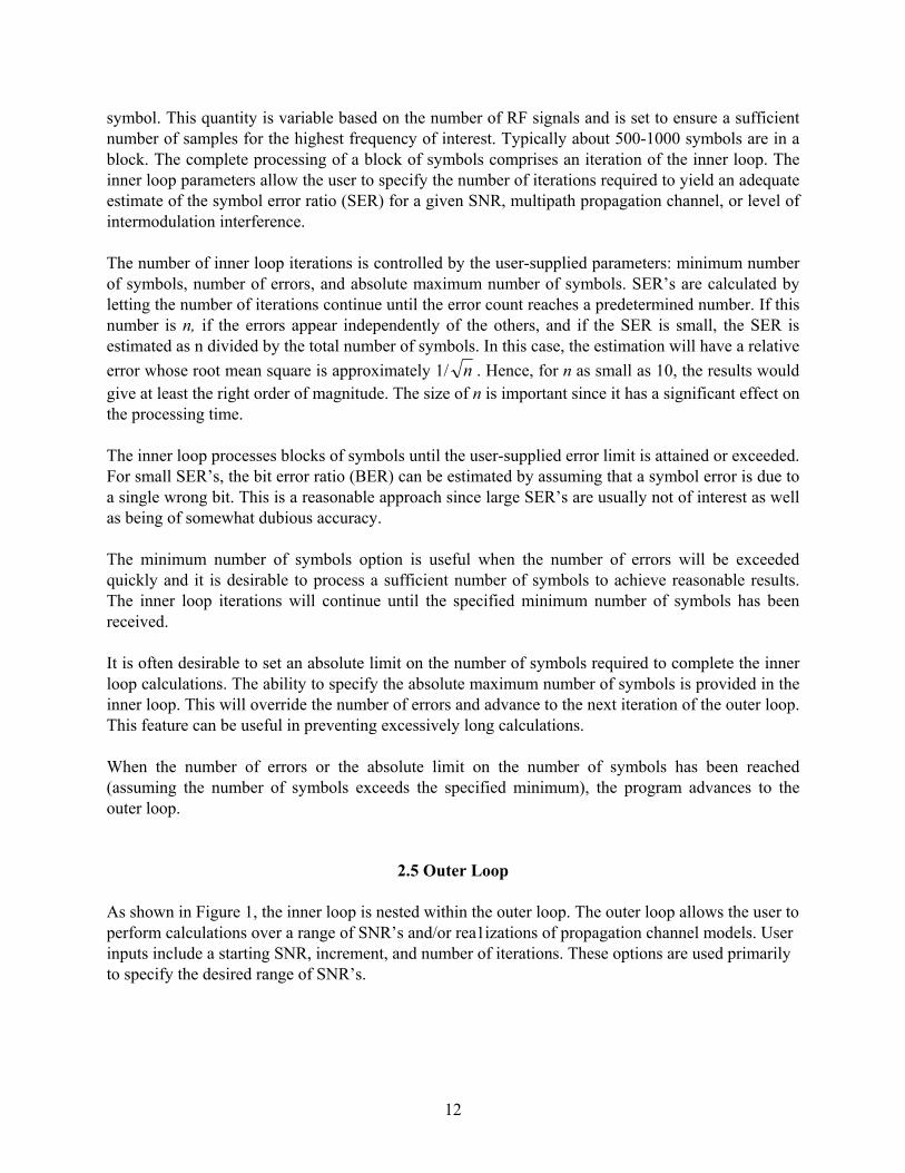
3.1 The Additive White Gaussian Noise Channel As a baseline, the model can be used to calculate symbol (or bit) error probabilities for a linear amplifier and an ideal propagation channel. Here, ideal propagation channel means that the signal is subject to additive white Gaussian noise (AWGN) only (no multipath). In this case, theoretical analysis is tractable, which provides a reality check for the simulation. Figure 8 shows the symbol error probability as a function of SNR for a single RF signal using 64QAM and 64TCM. The bandwidth was set at 7.2 MHz (20% guard) and the transmitter filter rolloff was set at 50% (4-Mbaud symbol rate). For this calculation, the maximum number of errors was set at 20.

3.2 Nonlinear Amplifier Proposed systems operating in the EHF band (LMDS) use nonlinear amplifiers that can cause signal distortion (primarily due to intermodulation). As indicated in Section 2, the simulation model includes nonlinear characteristics that approximate the behavior of a TWTA In particular, the user

14

Figure 8. Ideal channel symbol error probabilities

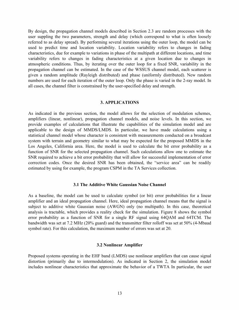
for 64QAM and 64TCM. can calculate SER as a function of the carrier-to-intermodulation ratio (C/I), or for the case of an AWGN channel, carrier-to-intermodulation plus noise. For this application, the user selects the desired input backoff. In this case, the carrier-to-intermodulation ratio (plus noise) is calculated along with the SER. As an example, symbol error calculations for the center carrier of a three-carrier system (RF bandwidth of 7.2 MHz, 50% transmitter filter rolloff, 20% guard band, 64QAM/64TCM) are shown in Figure 9. For these calculations, an equalizer was used and AWGN was not included. Note that this C/I is estimated for a particular set of signal specifications and amplifier backoff.

Figure 9. Symbol error ratio as a result of intermodulation

for 64QAM and 64TCM.

15

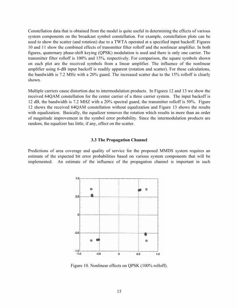
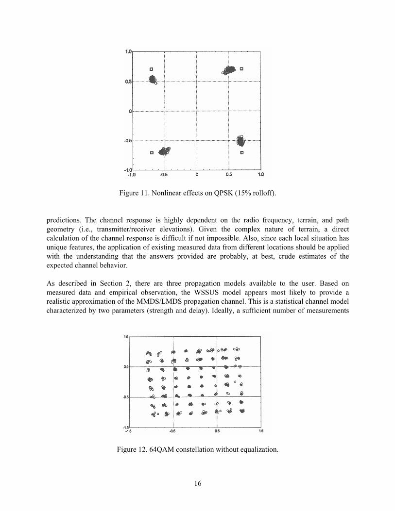
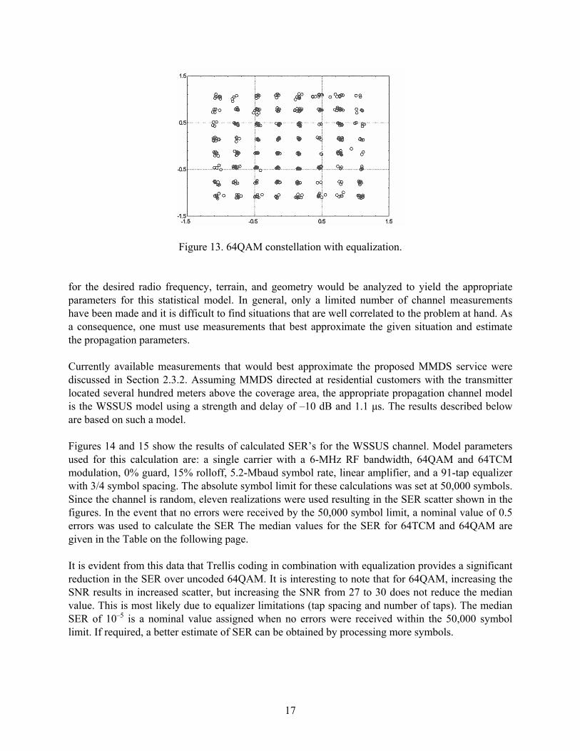
Constellation data that is obtained from the model is quite useful in determining the effects of various system components on the broadcast symbol constellation. For example, constellation plots can be used to show the scatter (and rotation) due to a TWTA operated at a specified input backoff. Figures 10 and 11 show the combined effects of transmitter filter rolloff and the nonlinear amplifier. In both figures, quaternary phase-shift keying (QPSK) modulation is used and there is only one carrier. The transmitter filter rolloff is 100% and 15%, respectively. For comparison, the square symbols shown on each plot are the received symbols from a linear amplifier. The influence of the nonlinear amplifier using 6-dB input backoff is readily apparent (rotation and scatter). For these calculations, the bandwidth is 7.2 MHz with a 20% guard. The increased scatter due to the 15% rolloff is clearly shown. Multiple carriers cause distortion due to intermodulation products. In Figures 12 and 13 we show the received 64QAM constellation for the center carrier of a three carrier system. The input backoff is 12 dB, the bandwidth is 7.2 MHZ with a 20% spectral guard, the transmitter rolloff is 50%. Figure 12 shows the received 64QAM constellation without equalization and Figure 13 shows the results with equalization. Basically, the equalizer removes the rotation which results in more than an order of magnitude improvement in the symbol error probability. Since the intermodulation products are random, the equalizer has little, if any, effect on the scatter.

3.3 The Propagation Channel Predictions of area coverage and quality of service for the proposed MMDS system requires an estimate of the expected bit error probabilities based on various system components that will be implemented. An estimate of the influence of the propagation channel is important in such

Figure 10. Nonlinear effects on QPSK (100% rolloff).

16

Figure 11. Nonlinear effects on QPSK (15% rolloff). predictions. The channel response is highly dependent on the radio frequency, terrain, and path geometry (i.e., transmitter/receiver elevations). Given the complex nature of terrain, a direct calculation of the channel response is difficult if not impossible. Also, since each local situation has unique features, the application of existing measured data from different locations should be applied with the understanding that the answers provided are probably, at best, crude estimates of the expected channel behavior. As described in Section 2, there are three propagation models available to the user. Based on measured data and empirical observation, the WSSUS model appears most likely to provide a realistic approximation of the MMDS/LMDS propagation channel. This is a statistical channel model characterized by two parameters (strength and delay). Ideally, a sufficient number of measurements

Figure 12. 64QAM constellation without equalization.

17

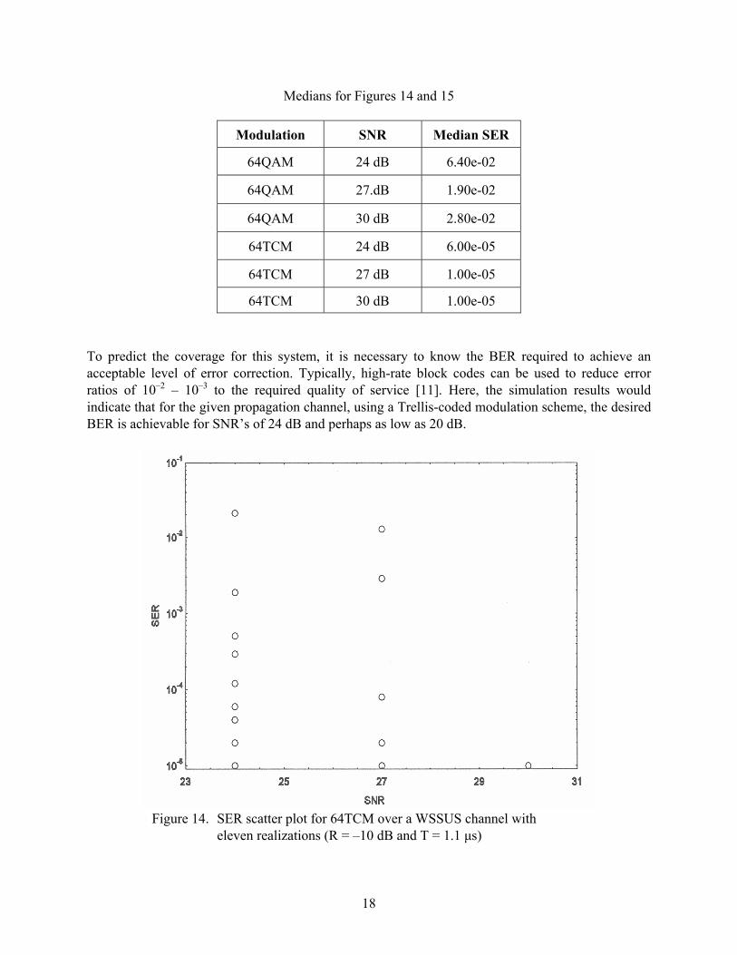
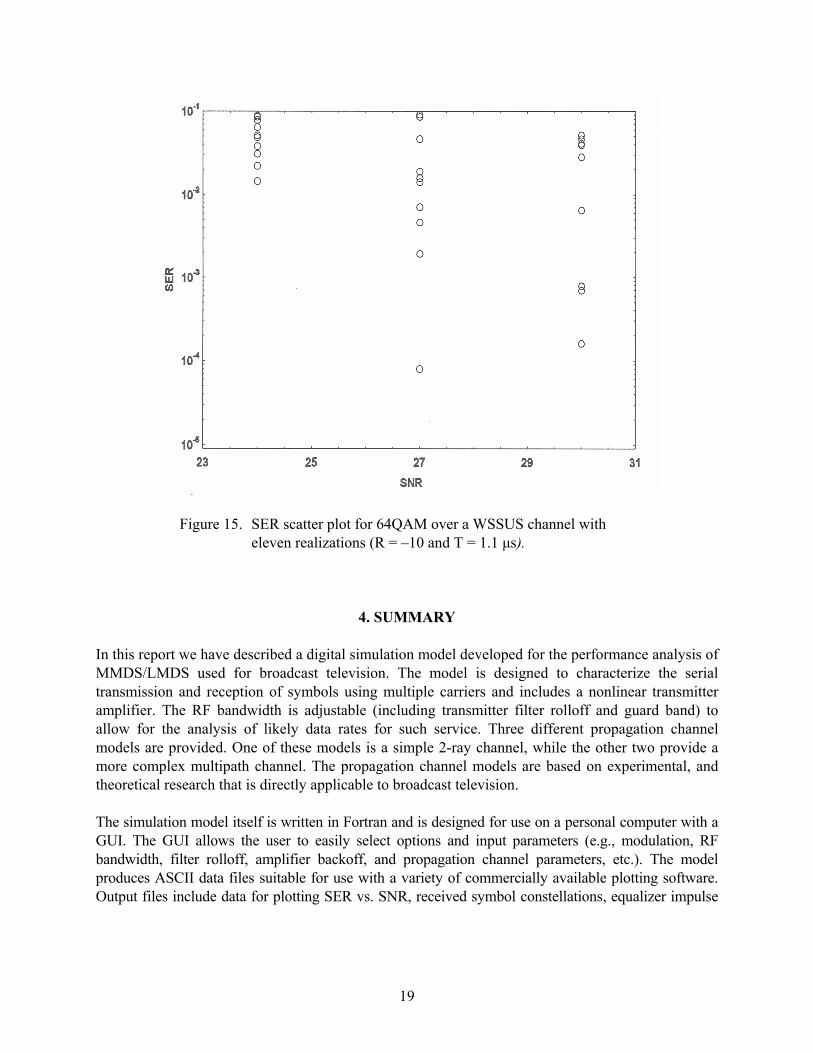
Figure 13. 64QAM constellation with equalization. for the desired radio frequency, terrain, and geometry would be analyzed to yield the appropriate parameters for this statistical model. In general, only a limited number of channel measurements have been made and it is difficult to find situations that are well correlated to the problem at hand. As a consequence, one must use measurements that best approximate the given situation and estimate the propagation parameters. Currently available measurements that would best approximate the proposed MMDS service were discussed in Section 2.3.2. Assuming MMDS directed at residential customers with the transmitter located several hundred meters above the coverage area, the appropriate propagation channel model is the WSSUS model using a strength and delay of –10 dB and 1.1 µs. The results described below are based on such a model. Figures 14 and 15 show the results of calculated SER’s for the WSSUS channel. Model parameters used for this calculation are: a single carrier with a 6-MHz RF bandwidth, 64QAM and 64TCM modulation, 0% guard, 15% rolloff, 5.2-Mbaud symbol rate, linear amplifier, and a 91-tap equalizer with 3/4 symbol spacing. The absolute symbol limit for these calculations was set at 50,000 symbols. Since the channel is random, eleven realizations were used resulting in the SER scatter shown in the figures. In the event that no errors were received by the 50,000 symbol limit, a nominal value of 0.5 errors was used to calculate the SER The median values for the SER for 64TCM and 64QAM are given in the Table on the following page. It is evident from this data that Trellis coding in combination with equalization provides a significant reduction in the SER over uncoded 64QAM. It is interesting to note that for 64QAM, increasing the SNR results in increased scatter, but increasing the SNR from 27 to 30 does not reduce the median value. This is most likely due to equalizer limitations (tap spacing and number of taps). The median SER of 10–5 is a nominal value assigned when no errors were received within the 50,000 symbol limit. If required, a better estimate of SER can be obtained by processing more symbols.

18

Medians for Figures 14 and 15

Modulation SNR Median SER

64QAM 24 dB 6.40e-02

64QAM 27.dB 1.90e-02

64QAM 30 dB 2.80e-02

64TCM 24 dB 6.00e-05

64TCM 27 dB 1.00e-05

64TCM 30 dB 1.00e-05 To predict the coverage for this system, it is necessary to know the BER required to achieve an acceptable level of error correction. Typically, high-rate block codes can be used to reduce error ratios of 10–2 – 10–3 to the required quality of service [11]. Here, the simulation results would indicate that for the given propagation channel, using a Trellis-coded modulation scheme, the desired BER is achievable for SNR’s of 24 dB and perhaps as low as 20 dB.

Figure 14. SER scatter plot for 64TCM over a WSSUS channel with

eleven realizations (R = –10 dB and T = 1.1 µs)

19

Figure 15. SER scatter plot for 64QAM over a WSSUS channel with

eleven realizations (R = –10 and T = 1.1 µs).

4. SUMMARY In this report we have described a digital simulation model developed for the performance analysis of MMDS/LMDS used for broadcast television. The model is designed to characterize the serial transmission and reception of symbols using multiple carriers and includes a nonlinear transmitter amplifier. The RF bandwidth is adjustable (including transmitter filter rolloff and guard band) to allow for the analysis of likely data rates for such service. Three different propagation channel models are provided. One of these models is a simple 2-ray channel, while the other two provide a more complex multipath channel. The propagation channel models are based on experimental, and theoretical research that is directly applicable to broadcast television. The simulation model itself is written in Fortran and is designed for use on a personal computer with a GUI. The GUI allows the user to easily select options and input parameters (e.g., modulation, RF bandwidth, filter rolloff, amplifier backoff, and propagation channel parameters, etc.). The model produces ASCII data files suitable for use with a variety of commercially available plotting software. Output files include data for plotting SER vs. SNR, received symbol constellations, equalizer impulse

20

response, and channel impulse response. The constellation and impulse response data are quite useful for analyzing how changes in user inputs affect overall system performance. We have also provided the results of sample calculations which are relevant to MMDS and LMDS service. Estimation of a propagation channel is of particular interest since it is applicable to the proposed MMDS services in southern California. Existing measurements using similar frequencies and path geometries were evaluated. Based on judgement and experience, we determined that measurements that most closely fit the geometry and usage (6-MHz broadcast television) were most applicable even though the frequency was lower than the proposed system. Using the theoretical channel model developed from this suite of measured data (WSSUS), we found that with equalization, an inner (Trellis) code of rate 5/6, and an SNR of 24 dB yields a BER that will allow for the effective use of outer (e.g., Reed Solomon) error correction codes. For many realizations of the propagation channel the omission of the inner code resulted in significantly larger BER’s, which may not achieve the threshold necessary for outer codes. Based on this analysis, the required SNR (including applicable fade margins) can be estimated and coverage predictions can be made using the CSPM available from TA Services. This model includes the effects of terrain and “slow fading.”

5. REFERENCES [1] B.J. Leland, Digital Filters and Signal Processing, Hingham, MA: Kluwer Academic

Publishers, 1986, pp. 90, 130. [2] G. Ungerboeck, “Trellis-coded modulation with redundant signal sets,” IEEE

Communications Magazine, vol. 25, no. 2, pp. 5-21, 1987. [3] CCITT (The International Telegraph and Telephone Consultative Committee), Data

communication over the telephone network, Blue Book, Fascicle VIII.1, Recommendation vol. 33, pp. 252-256, 1989.

[4] G.D. Forney, “The Viterbi algorithm,” in Proc. IEEE, vol. 61, no. 3, pp. 268-278, 1973. [5] M. Sablatash, J. L. Lodge, and K. W. Moreland, “Theory and methods for design of pulse

shapes for broadcast teletext,” IEEE Trans. Broadcasting, vol. 35, no. 1, pp. 40-55, 1989. [6] A.A.M. Saleh, “Frequency-independent and frequency-dependent nonlinear models of TWT

amplifiers,” IEEE Trans. Communications, vol. COM-29, no. 11, pp. 1715-1720, 1981. [7] G.L. Turin, “A statistical model of urban multipath propagation,” IEEE Trans. Vehicular

Technology, vol. VT-21, no. 1, pp. 1-9, 1972. [8] H. Hashemi, “Simulation of the urban radio propagation channel,” IEEE Trans. Vehicular

Technology, vol. VT-28, no. 3, pp. 213-225, 1979.

21

[9] G. Hufford, “A characterization of the multipath in the HDTV channel,” IEEE Trans. Broadcasting, vol. 38, no. 4, pp. 252-254, 1992.

[10] J.A Wepman, J.R Hoffman, and L.H. Loew, “Analysis of impulse response measurements for

PCS channel modelling applications,” IEEE Trans. Vehicular Technology, vol. 44, no. 3, pp. 613-620, 1995.

[11] A.M. Michelson and A.H. Levesque, “Error-control Techniques for Digital Communication,

New York, NY: John Wiley & Sons, 1985, pp. 382.

23

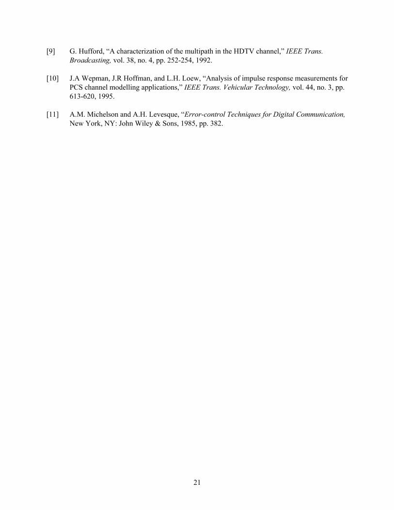
APPENDIX A: SIMULATION MODEL USER'S GUIDE The digital simulation program is written for a personal computer using a GUI. The program is started by double clicking on the selected icon. A window containing the main menu as shown in Figure A-1 will appear. Each button opens a window for the input parameters described in Section 2. This window will remain open until the user clicks on the Stop or Run option. The Stop option stops execution of the program, and the Run option executes the program for the selected parameters. For most options, a brief explanation will appear at the bottom of the window when the cursor is moved to a particular button or edit box (see Figure A-4 below for an example). Clicking on the RF Signal button opens the window shown in Figure A-2 below. The user selects the modulation (push button format) and enters signal parameters. Default values are shown in the edit boxes. The Tab key can be used to step through the options. Parameters are set once the user clicks on exit (this closes the window). Each window can be revisited (and parameters changed) as often as desired prior to choosing the run option of the main menu. Windows containing user options for the Amplifier, Channel, Inner Loop, and Outer Loop are shown below (Figures A-3 through A-6). In each case, push buttons and/or edit boxes are provided for user input. As before, user selections are registered upon exiting the window. Each window can be reopened and changes can be made as often as desired before the program is run.

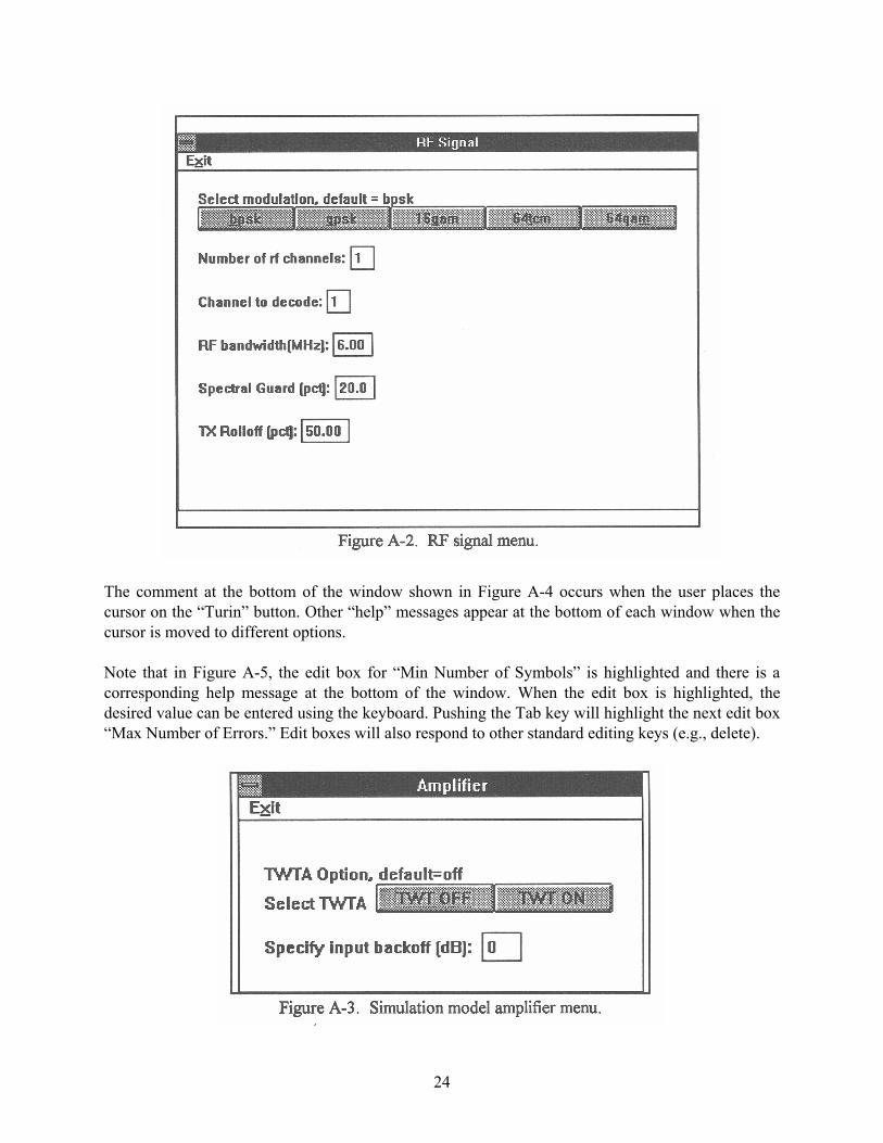
24

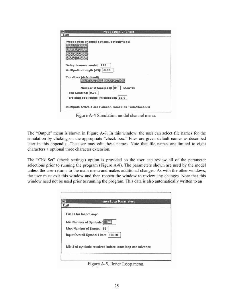
The comment at the bottom of the window shown in Figure A-4 occurs when the user places the cursor on the “Turin” button. Other “help” messages appear at the bottom of each window when the cursor is moved to different options. Note that in Figure A-5, the edit box for “Min Number of Symbols” is highlighted and there is a corresponding help message at the bottom of the window. When the edit box is highlighted, the desired value can be entered using the keyboard. Pushing the Tab key will highlight the next edit box “Max Number of Errors.” Edit boxes will also respond to other standard editing keys (e.g., delete).

25

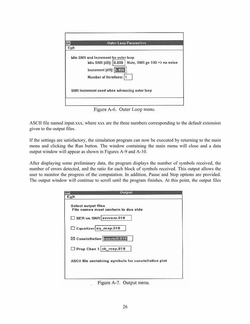
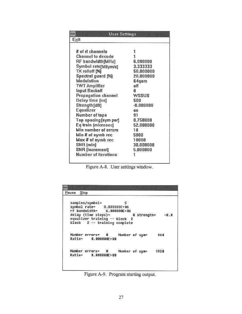
The “Output” menu is shown in Figure A-7. In this window, the user can select file names for the simulation by clicking on the appropriate “check box.” Files are given default names as described later in this appendix. The user may edit these names. Note that file names are limited to eight characters + optional three character extension. The “Chk Set” (check settings) option is provided so the user can review all of the parameter selections prior to running the program (Figure A-8). The parameters shown are used by the model unless the user returns to the main menu and makes additional changes. As with the other windows, the user must exit this window and then reopen the window to review any changes. Note that this window need not be used prior to running the program. This data is also automatically written to an

26

ASCII file named input.xxx, where xxx are the three numbers corresponding to the default extension given to the output files. If the settings are satisfactory, the simulation program can now be executed by returning to the main menu and clicking the Run button. The window containing the main menu will close and a data output window will appear as shown in Figures A-9 and A-10. After displaying some preliminary data, the program displays the number of symbols received, the number of errors detected, and the ratio for each block of symbols received. This output allows the user to monitor the progress of the computation. In addition, Pause and Stop options are provided. The output window will continue to scroll until the program finishes. At this point, the output files

27

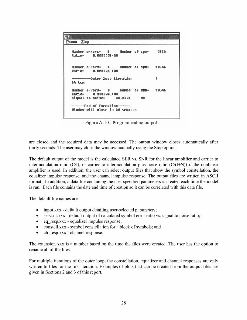
28

are closed and the required data may be accessed. The output window closes automatically after thirty seconds. The user may close the window manually using the Stop option. The default output of the model is the calculated SER vs. SNR for the linear amplifier and carrier to intermodulation ratio (C/I), or carrier to intermodulation plus noise ratio (C/(I+N)) if the nonlinear amplifier is used. In addition, the user can select output files that show the symbol constellation, the equalizer impulse response, and the channel impulse response. The output files are written in ASCII format. In addition, a data file containing the user specified parameters is created each time the model is run. Each file contains the date and time of creation so it can be correlated with this data file. The default file names are:

• input.xxx - default output detailing user-selected parameters; • servsnr.xxx - default output of calculated symbol error ratio vs. signal to noise ratio; • eq_resp.xxx - equalizer impulse response; • constell.xxx - symbol constellation for a block of symbols; and • ch_resp.xxx - channel response.

The extension xxx is a number based on the time the files were created. The user has the option to rename all of the files. For multiple iterations of the outer loop, the constellation, equalizer and channel responses are only written to files for the first iteration. Examples of plots that can be created from the output files are given in Sections 2 and 3 of this report.

29

Most of the output files contain two columns of data that can be used to create two-dimensional “xy” plots. The channel response file contains several columns of data. The first column is time and the second column gives the magnitude of the channel. Typically this is the format in which channel response data is given. The magnitude of the channel response is given in dB. The other columns of data contain the real and imaginary components of both the unfiltered channel response and the filtered channel response. This data is linear, while the final two columns of data are the filtered channel response in dB. The additional data was used for diagnostic purposes and was maintained as an output that can be reviewed if desired. On rare occasions, a coprocessor fault occurs. This appears to be connected with Windows® memory management and is most likely to occur when using applications which require significant system resources. Exiting Windows® and restarting the program will resolve the problem. Another error experienced on an infrequent basis is the argument of the logarithm function being zero. As the error is quite infrequent, its source has not been identified. Typically, the logarithm function is used to calculate decibels. In this case, the program must be restarted.