A duty cycle optimization based hybrid maximum power point tracking technique for photovoltaic systems

Electrical Power and Energy Systems 59 (2014) 141–154

Contents lists available at ScienceDirect

Electrical Power and Energy Systems

journal homepage: www.elsevier .com/locate / i jepes

A duty cycle optimization based hybrid maximum power point trackingtechnique for photovoltaic systems

http://dx.doi.org/10.1016/j.ijepes.2014.02.0090142-0615/� 2014 Elsevier Ltd. All rights reserved.

⇑ Corresponding author at: LIM – Mechatronics Lab, Politecnico di Torino, CorsoDuca degli Abruzzi, 24 – 10129 Torino, Italy. Tel.: +39 3453249491; fax: +39 0110907963.

E-mail addresses: [email protected], [email protected] (A. Murtaza).

Ali Murtaza a,b,⇑, Marcello Chiaberge a,c, Mirko De Giuseppe a,c, Diego Boero a,b

a LIM – Mechatronics Laboratory, Politecnico di Torino, Italyb Department of Mechanical and Aerospace Engineering, Politecnico di Torino, Italyc Department of Electronics and Telecommunication Engineering, Politecnico di Torino, Italy

a r t i c l e i n f o

Article history:Received 24 April 2013Received in revised form 15 February 2014Accepted 18 February 2014

Keywords:Photovoltaic (PV) systemsMaximum power point tracking (MPPT)techniquePerturb & observe (P&O)Fraction open-circuit voltage (FOCV)Hybrid MPPT

a b s t r a c t

Photovoltaic (PV) energy has witnessed tremendous growth in the recent past. PV system exhibits the IVcurve, which varies non-linearly according to immediate weather conditions. Maximum power pointtracking (MPPT) technique is an essential part of PV system which tracks the unique maximum powerpoint (MPP) on its IV curve. In this paper, a new MPPT is proposed which is equipped with duty cycle(D) optimization method. The proposed method works in three stages containing hybrid mechanism oftwo basic techniques i.e. perturb & observe (P&O) and fractional open-circuit voltage (FOCV). D-optimi-zation scheme enhances the performance of the proposed technique under varying weather conditionscompared to past MPPTs. While hybrid mechanism helps the technique to quickly focus the MPP withnegligible power loss oscillations under steady weather conditions. For stable operation of MPPTalgorithm, instrumentation and measurement issues of PV system have been addressed. A new evalua-tion criteria is proposed for MPPT algorithms. Finally, the proposed MPPT and other techniques have beensimulated in Matlab/Simulink under various weather conditions. Simulation analysis confirms thesuperior performance of the proposed algorithm compared to other MPPTs. The evaluation criteriareveals that the PV array operates at an efficiency of 99.9% under steady conditions while under dynamicweather conditions the operational efficiency of the PV array is always in excess of 90% with the aid of theproposed technique.

� 2014 Elsevier Ltd. All rights reserved.

1. Introduction

In recent past, renewable energy systems get substantialpopularity because of its clean nature and decreasing cost.Amongst these, photovoltaic (PV) system receives great attentionbecause of its technology development, reduced cost and reliablesun source. The basic unit of a PV system is a PV module. For de-sired power/voltage levels, PV modules are connected together ina series/parallel configuration to make a PV plant. The main draw-back of PV plant is that they generate non-linear IV curves whichvary according to immediate weather conditions. Also, PV plantoperating point on its IV curve depends upon the load. Therefore,some mechanism is required which has to deal with dynamic/static weather conditions and accordingly operate the load in suchmanner that the PV plant will operate on its maximum power

point (MPP). Such mechanism is known as maximum power pointtracking (MPPT) technique.

Many researchers developed different MPPT techniques andsome of them are surveyed by [1]. These techniques are varyingfrom conventional low complex techniques like perturb & observe(P&O), incremental conductance (IC), fractional open-circuit volt-age (FOCV) etc. to medium complex techniques [2–6] to high com-plex techniques like fuzzy logic [7], neural networks [8] etc. Tilldate, no agreement is developed amongst the researchers thatwhich technique is best [9]. However P&O is the most usedtechnique because of its less complexity, low cost and implemen-tation ease. But this technique may struggle in varying weatherconditions and always produce power loss oscillations aroundMPP in static weather [2–4,9]. Many researchers optimize P&Owith different ideas [2–5,10–18].

Techniques [2–4] utilize a hybrid mechanism of two basictechniques which are FOCV and P&O. However technique [2] ismore efficient than [4] but it requires the temperature sensing,which increases the implementation cost of the PV system. Workpresented in [10] utilizes two PI controllers to optimize P&O, one

http://crossmark.crossref.org/dialog/?doi=10.1016/j.ijepes.2014.02.009&domain=pdf

http://dx.doi.org/10.1016/j.ijepes.2014.02.009

mailto:[email protected]

mailto:[email protected]

http://dx.doi.org/10.1016/j.ijepes.2014.02.009

http://www.sciencedirect.com/science/journal/01420615

http://www.elsevier.com/locate/ijepes

142 A. Murtaza et al. / Electrical Power and Energy Systems 59 (2014) 141–154

is to calculate the voltage perturb and other one for the converterto generate the duty cycle. This technique has a drawback of algo-rithm complexity as tuning of two PI controllers is required. A cur-rent-based sliding mode MPPT algorithm is presented in [11] tooptimize the P&O. However, it uses an additional voltage compen-sation loop to deal with fast irradiance variations. To optimize theP&O, a three point weight comparison based MPPT is presented in[18]. Since this algorithm requires three point information todecide the next step, the convergence speed of this algorithm iscompromised.

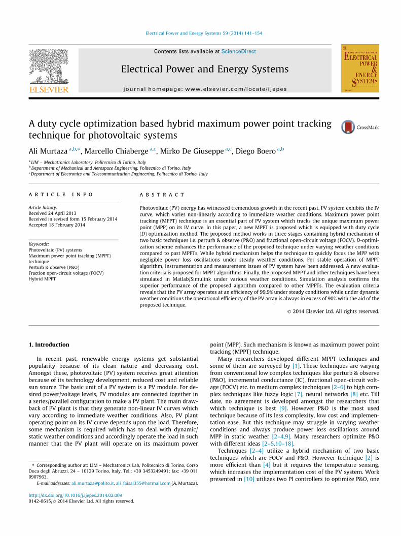
Proposed technique also tries to optimize P&O and thereforeadopts the hybrid approach by utilizing two basic techniques i.e.P&O and FOCV. Flowchart of P&O algorithm is shown in Fig. 1. Itsimply perturbs the voltage in one direction and then observes thatwhether new power is greater than previous power. If it is true,then it will continue in the same direction, otherwise it will per-turb the voltage in the opposite direction. While, FOCV revolvesaround a simple relation as described by Eq. (1):

Vpv ) Vmpp ¼ k� Voc ð1Þ

It takes advantage of the fact that normally maximum power pointvoltage (Vmpp) is near to open-circuit voltage (Voc) of PV module.Therefore Vmpp is estimated by the product of Voc and factor k (nor-mally varies between 0.7 and 0.8) and then set the operating volt-age (Vpv) of a PV system at Vmpp. Since temperature producesmajor effect in Voc and irradiance produces minor change in Voc,FOCV periodically measures Voc to readjust Vpv. Techniques [2–4]also utilizes the hybrid approach with same two techniques. Theproposed technique is influenced from [3]. Work presented in[19] compared MPPT techniques from almost every field i.e. opti-mized P&O, optimized IC, hybrid MPPT‘s, fuzzy logic and neural net-works etc. and declared hybrid MPPT technique [2] as one of themost efficient.

In this paper, a new duty cycle (D) optimization method isdeveloped. It is inducted in proposed MPPT to enhance its dynamicresponse under varying weather conditions i.e. fast convergence toMPP while reducing power loss. The proposed technique utilizestwo sensors i.e. watt-meter & volt-meter thus making it cost effec-tive. Some modifications in instrumentation and issues relatedwith measurement of PV system parameters have been addressed.Simulations have been performed in Matlab/Simulink on variousweather conditions. It can be confirmed from simulation analysisthat proposed method is quite able to track MPP efficiently evenunder fast changing weather conditions. Also, it exhibits negligiblepower loss oscillation under static weather conditions. Theproposed technique is compared with hybrid technique [2] andbasic P&O. Comparison results indicate that the proposed methodoutperforms others.

Fig. 1. Flowchart of conventional P&O algorithm.

2. PV module characteristics

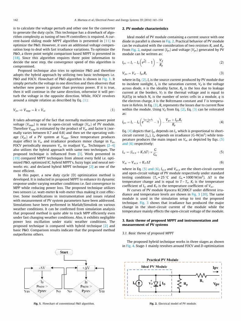
Ideal model of PV module containing a current source with onediode in parallel is shown in Fig. 2. Practical behavior of PV modulecan be evaluated with the consideration of two resistors Rs and Rp.From Fig. 2, output current (Ipv) and voltage (Vpv) generated by PVmodule can be written as:

Ipv ¼ Is � Io eVdnVt � 1

� �� Vd

Rpð2Þ

Vpv ¼ Vd � IpvRs ð3Þ

where in Eq. (2), Is is the source current produced by PV module dueto incident sunlight, Io is the saturation current, Vd is the voltageacross diode, n is the ideality factor, Rp is the loss due to leakagecurrent at the borders, VT is the thermal voltage and is equal toNskT/q in which Ns is the number of series cells in a module, q isthe electron charge, k is the Boltzmann constant and T is tempera-ture in Kelvin. In Eq. (3), Rs represents the losses due to current flowwithin the module. Using Vd from Eq. (2), Eq. (3) can be reiteratedas:

Ipv ¼ Is � Io eVpvþIpv Rs

nVt � 1� �

� Vpv þ IpvRs

Rpð4Þ

Eq. (4) depicts that Ipv depends on Is, which is proportional to short-circuit current (Isc). Isc depends on irradiance (G-W/m2) while tem-perature produces the main impact on Voc as depicted by Eqs. (5)and (6) respectively:

Isc ¼ ðIsc;n þ KIDTÞ � GGn

ð5Þ

Voc ¼ Voc;n þ KVDT ð6Þ

where in Eq. (5) and (6), Isc,n and Voc,n are the short-circuit currentand open-circuit voltage of PV module respectively under standardtesting conditions (Tn = 25 �C and Gn = 1000 W/m2). DT is thetemperature change and is equal to T – Tn. KI is the temperaturecoefficient of Isc and KV is the temperature coefficient of Voc.

IV curves of PV module Kyocera KC200GT under different irra-diance and temperature levels are shown in Fig. 3 [20]. The samemodule is used in the simulation setup to test the proposedtechnique. Fig. 3 shows that irradiance has produced the majorchange in the short-circuit current of the module while thetemperature mainly effects the open-circuit voltage of the module.

3. Basic theme of proposed MPPT and instrumentation andmeasurement of PV systems

3.1. Basic theme of proposed MPPT

The proposed hybrid technique works in three stages as shownin Fig. 4. Stage-1 mainly revolves around FOCV and D-optimization

Fig. 2. Electrical model of PV module.

Fig. 3. IV curves of KC200GT at different irradiance (left fig) and temperature (right fig) levels.

Fig. 4. Basic theme of proposed MPPT.

A. Murtaza et al. / Electrical Power and Energy Systems 59 (2014) 141–154 143

method. Role of stage-1 is to estimate the maximum power pointvoltage (Vmpp) and then throw the operating voltage (Vpv) nearVmpp. First open-circuit voltage (Voc) is measured and then Vmpp iscalculated by multiplying factor k with Voc. Finally algorithm triesto make Vpv equal to kVoc through D-optimization method. Afterthat, software enters in stage-2 containing hybrid mechanism ofP&O and FOCV. Here it enjoys the modified P&O with smaller stepsize compared to conventional P&O to reach MPP precisely andthen enter into the next stage. In stage-3, algorithm reached theMPP and is static at that point. Since k value normally varies from0.7 to 0.8, its value is dynamically re-adjusted according to PVplant behavior. At any stage if there is change in atmosphere,algorithm rolls back to stage-1.

3.2. Instrumentation and measurement of PV Systems

In PV systems, DC–DC converter (buck, boost or buck-boost etc.)is present between PV array/plant and the load. A system architec-ture of a stand-alone PV system with buck converter is shown inFig. 5. PV array reaches its MPP when the output load (Rout)becomes equal to the internal impedance (Rimp,pv) of the PV array.With different atmospheric conditions, Rimp,pv of PV array gets

changed all the time. However Rout is not changed accordingly onits own. For that MPPT designer utilizes DC–DC converter to varyRout. Relation between input voltage (Vin) and output voltage (Vout)of a buck converter shown in Fig. 5 can be written as:

Vout ¼ DVin ð7Þ

where D means duty cycle. With 100% efficiency, we can assumePin = Pout, therefore

VinIin ¼ VoutIout )ðVinÞ2

Rin¼ ðVoutÞ2

Routð8Þ

By using Eq. (7), Eq. (8) can be rewritten as:

Rin ¼1

D2 Rout ð9Þ

It is clear from Eq. (9) that Rout and Rin are two parameters of theconverter. Rout itself may remain the same, but load seen by PVmodule i.e. Rin can be varied with the help of D. Actually by chang-ing D, Rin is varied and in response PV module changes its operatingvoltage (Vpv). It is the responsibility of the MPPT algorithm to set Dat such optimized value (Dmpp) that Rin matches the internal imped-ance of the array (Rimp,pv). At this stage, the module starts operatingat the maximum power point voltage (Vmpp) which delivers themaximum power. Eqs. (10) and (11) describe this mechanism:

At non�MPP : Rin ¼1

D2 Rout ) Rin – Rimp;pv ; Vpv – Vmpp ð10Þ

At MPP : Rin ¼1

D2mpp

Rout ) Rin ¼ Rimp;pv ; Vpv ¼ Vmpp ð11Þ

3.2.1. Open-circuit voltage (Voc) measurement issuesIn the first stage as shown in Fig. 4, proposed technique needs to

measure open-circuit voltage (Voc). One way is to measure it di-rectly from the PV array by disconnecting it from the load and thenreconnect it. But it means the loss of power during Voc measure-ment. Technique [2] finds out the alternate way by utilizing tem-perature sensor with a specific relation. It does not require theshedding of PV system from the load. However, this method ismore of an estimation rather than actual measurement of Voc, soaccuracy may degrade. Also, it is difficult to manage large PV plant

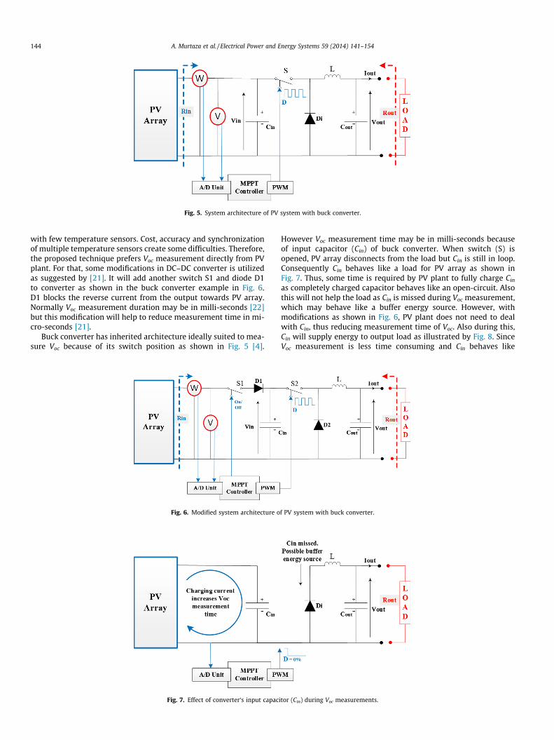
Fig. 5. System architecture of PV system with buck converter.


with few temperature sensors. Cost, accuracy and synchronizationof multiple temperature sensors create some difficulties. Therefore,the proposed technique prefers Voc measurement directly from PVplant. For that, some modifications in DC–DC converter is utilizedas suggested by [21]. It will add another switch S1 and diode D1to converter as shown in the buck converter example in Fig. 6.D1 blocks the reverse current from the output towards PV array.Normally Voc measurement duration may be in milli-seconds [22]but this modification will help to reduce measurement time in mi-cro-seconds [21].

Buck converter has inherited architecture ideally suited to mea-sure Voc because of its switch position as shown in Fig. 5 [4].

Fig. 6. Modified system architecture o

Fig. 7. Effect of converter‘s input capac

However Voc measurement time may be in milli-seconds becauseof input capacitor (Cin) of buck converter. When switch (S) isopened, PV array disconnects from the load but Cin is still in loop.Consequently Cin behaves like a load for PV array as shown inFig. 7. Thus, some time is required by PV plant to fully charge Cin

as completely charged capacitor behaves like an open-circuit. Alsothis will not help the load as Cin is missed during Voc measurement,which may behave like a buffer energy source. However, withmodifications as shown in Fig. 6, PV plant does not need to dealwith Cin, thus reducing measurement time of Voc. Also during this,Cin will supply energy to output load as illustrated by Fig. 8. SinceVoc measurement is less time consuming and Cin behaves like

f PV system with buck converter.

itor (Cin) during Voc measurements.

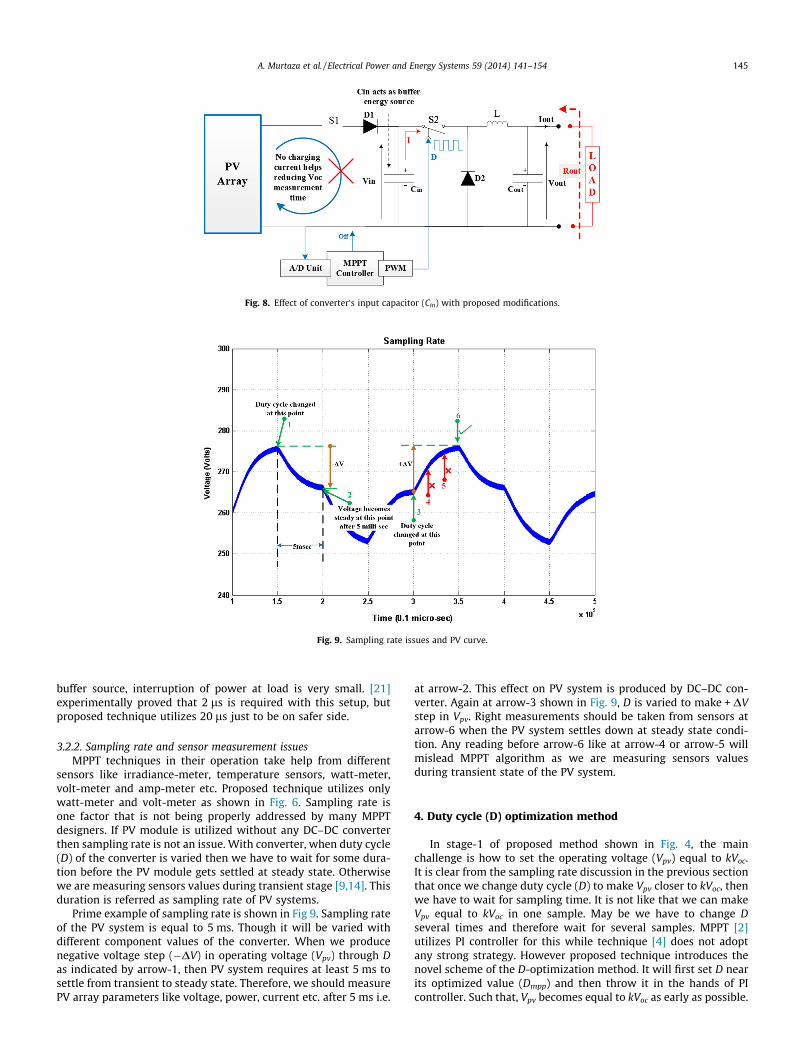
Fig. 8. Effect of converter‘s input capacitor (Cin) with proposed modifications.

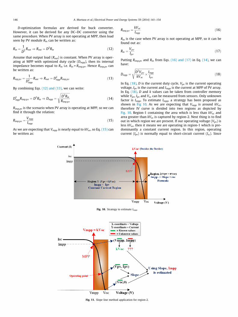
Fig. 9. Sampling rate issues and PV curve.


buffer source, interruption of power at load is very small. [21]experimentally proved that 2 ls is required with this setup, butproposed technique utilizes 20 ls just to be on safer side.

3.2.2. Sampling rate and sensor measurement issuesMPPT techniques in their operation take help from different

sensors like irradiance-meter, temperature sensors, watt-meter,volt-meter and amp-meter etc. Proposed technique utilizes onlywatt-meter and volt-meter as shown in Fig. 6. Sampling rate isone factor that is not being properly addressed by many MPPTdesigners. If PV module is utilized without any DC–DC converterthen sampling rate is not an issue. With converter, when duty cycle(D) of the converter is varied then we have to wait for some dura-tion before the PV module gets settled at steady state. Otherwisewe are measuring sensors values during transient stage [9,14]. Thisduration is referred as sampling rate of PV systems.

Prime example of sampling rate is shown in Fig 9. Sampling rateof the PV system is equal to 5 ms. Though it will be varied withdifferent component values of the converter. When we producenegative voltage step (�DV) in operating voltage (Vpv) through Das indicated by arrow-1, then PV system requires at least 5 ms tosettle from transient to steady state. Therefore, we should measurePV array parameters like voltage, power, current etc. after 5 ms i.e.

at arrow-2. This effect on PV system is produced by DC–DC con-verter. Again at arrow-3 shown in Fig. 9, D is varied to make + DVstep in Vpv. Right measurements should be taken from sensors atarrow-6 when the PV system settles down at steady state condi-tion. Any reading before arrow-6 like at arrow-4 or arrow-5 willmislead MPPT algorithm as we are measuring sensors valuesduring transient state of the PV system.

4. Duty cycle (D) optimization method

In stage-1 of proposed method shown in Fig. 4, the mainchallenge is how to set the operating voltage (Vpv) equal to kVoc.It is clear from the sampling rate discussion in the previous sectionthat once we change duty cycle (D) to make Vpv closer to kVoc, thenwe have to wait for sampling time. It is not like that we can makeVpv equal to kVoc in one sample. May be we have to change Dseveral times and therefore wait for several samples. MPPT [2]utilizes PI controller for this while technique [4] does not adoptany strong strategy. However proposed technique introduces thenovel scheme of the D-optimization method. It will first set D nearits optimized value (Dmpp) and then throw it in the hands of PIcontroller. Such that, Vpv becomes equal to kVoc as early as possible.


D-optimization formulas are derived for buck converter.However, it can be derived for any DC–DC converter using thesame procedure. When PV array is not operating at MPP, then loadseen by PV module Rin can be written as:

Rin ¼1

D2 Rout ) Rout ¼ D2Rin ð12Þ

Assume that output load (Rout) is constant. When PV array is oper-ating at MPP with optimized duty cycle (Dmpp), then its internalimpedance becomes equal to Rin i.e. Rin = Rimp,pv. Hence Rimp,pv canbe written as:

Rinp;pv ¼1

D2mpp

Rout ) Rout ¼ D2mppRimp;pv ð13Þ

By combining Eqs. (12) and (13), we can write:

D2mppRimp;pv ¼ D2Rin ) Dmpp ¼

ffiffiffiffiffiffiffiffiffiffiffiffiffiD2Rin

Rimp;pv

sð14Þ

Rimp,pv is the scenario when PV array is operating at MPP, so we canfind it through the relation:

Rimp;pv ¼Vmpp

Imppð15Þ

As we are expecting that Vmpp is nearly equal to kVoc, so Eq. (15) canbe written as:

Fig. 10. Strategy to

Fig. 11. Slope line method a

Rimp;pv ¼kVoc

Imppð16Þ

Rin is the case when PV array is not operating at MPP, so it can befound out as:

Rin ¼Vpv

Ipvð17Þ

Putting Rimp,pv and Rin from Eqs. (16) and (17) in Eq. (14), we canhave:

Dmpp ¼

ffiffiffiffiffiffiffiffiffiffiffiffiffiffiffiffiffiffiffiffiffiffiffiffiffiffiffiD2Vpv

kVoc� Impp

Ipv

sð18Þ

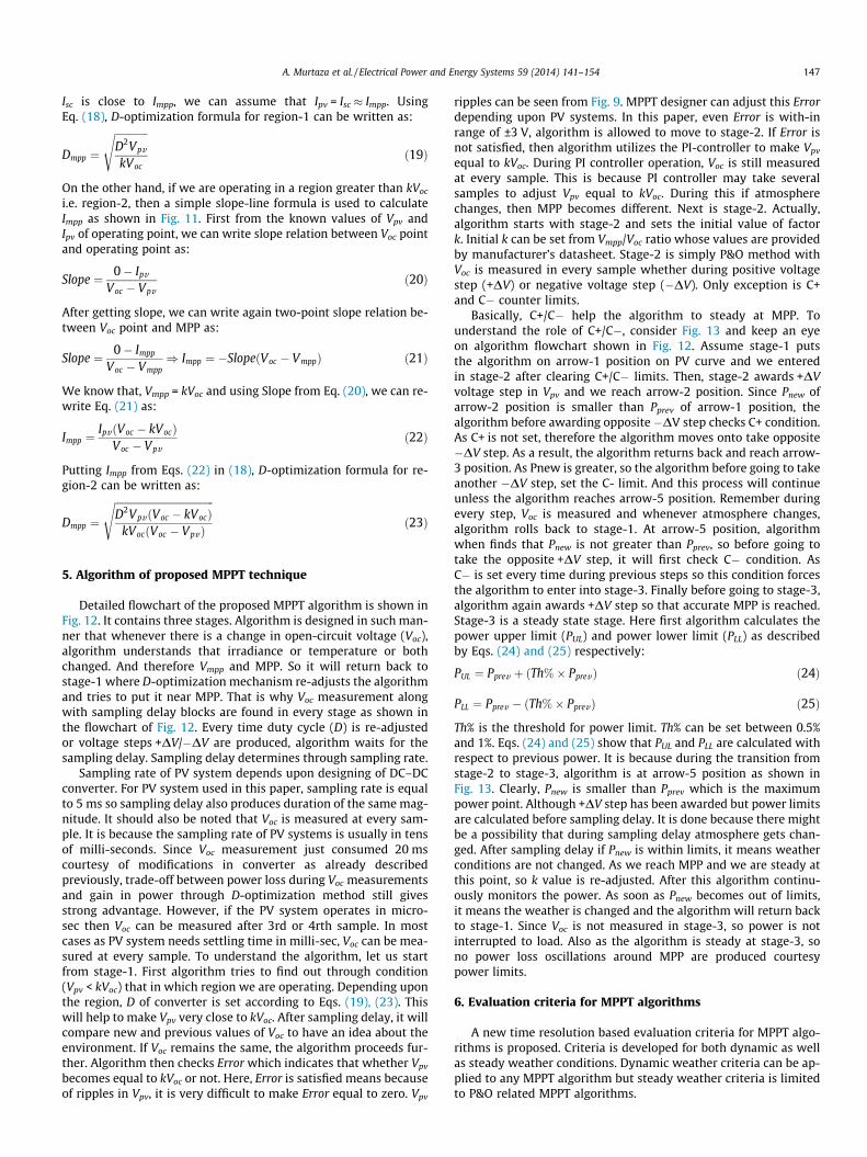
In Eq. (18), D is the current duty cycle, Vpv is the current operatingvoltage, Ipv is the current and Impp is the current at MPP of PV array.In Eq. (18), D and k values can be taken from controller memorywhile Vpv, Ipv and Voc can be measured from sensors. Only unknownfactor is Impp. To estimate Impp, a strategy has been proposed asshown in Fig 10. As we are expecting that Vmpp is around kVoc,therefore IV curve is divided into two regions as depicted byFig. 10. Region-1 containing the area which is less than kVoc andarea greater than kVoc is captured by region-2. Next thing is to findout in which region we are present. If our operating voltage (Vpv) isless kVoc, then it means we are operating in region-1 which is pre-dominantly a constant current region. In this region, operatingcurrent (Ipv) is normally equal to short-circuit current (Isc). Since

estimate Impp.

pplication for region-2.


Isc is close to Impp, we can assume that Ipv = Isc � Impp. UsingEq. (18), D-optimization formula for region-1 can be written as:

Dmpp ¼

ffiffiffiffiffiffiffiffiffiffiffiffiffiD2Vpv

kVoc

sð19Þ

On the other hand, if we are operating in a region greater than kVoc

i.e. region-2, then a simple slope-line formula is used to calculateImpp as shown in Fig. 11. First from the known values of Vpv andIpv of operating point, we can write slope relation between Voc pointand operating point as:

Slope ¼ 0� Ipv

Voc � Vpvð20Þ

After getting slope, we can write again two-point slope relation be-tween Voc point and MPP as:

Slope ¼ 0� Impp

Voc � Vmpp) Impp ¼ �SlopeðVoc � VmppÞ ð21Þ

We know that, Vmpp = kVoc and using Slope from Eq. (20), we can re-write Eq. (21) as:

Impp ¼IpvðVoc � kVocÞ

Voc � Vpvð22Þ

Putting Impp from Eqs. (22) in (18), D-optimization formula for re-gion-2 can be written as:

Dmpp ¼

ffiffiffiffiffiffiffiffiffiffiffiffiffiffiffiffiffiffiffiffiffiffiffiffiffiffiffiffiffiffiffiffiffiffiffiffiffiffiffiD2VpvðVoc � kVocÞ

kVocðVoc � VpvÞ

sð23Þ

5. Algorithm of proposed MPPT technique

Detailed flowchart of the proposed MPPT algorithm is shown inFig. 12. It contains three stages. Algorithm is designed in such man-ner that whenever there is a change in open-circuit voltage (Voc),algorithm understands that irradiance or temperature or bothchanged. And therefore Vmpp and MPP. So it will return back tostage-1 where D-optimization mechanism re-adjusts the algorithmand tries to put it near MPP. That is why Voc measurement alongwith sampling delay blocks are found in every stage as shown inthe flowchart of Fig. 12. Every time duty cycle (D) is re-adjustedor voltage steps +DV/�DV are produced, algorithm waits for thesampling delay. Sampling delay determines through sampling rate.

Sampling rate of PV system depends upon designing of DC–DCconverter. For PV system used in this paper, sampling rate is equalto 5 ms so sampling delay also produces duration of the same mag-nitude. It should also be noted that Voc is measured at every sam-ple. It is because the sampling rate of PV systems is usually in tensof milli-seconds. Since Voc measurement just consumed 20 mscourtesy of modifications in converter as already describedpreviously, trade-off between power loss during Voc measurementsand gain in power through D-optimization method still givesstrong advantage. However, if the PV system operates in micro-sec then Voc can be measured after 3rd or 4rth sample. In mostcases as PV system needs settling time in milli-sec, Voc can be mea-sured at every sample. To understand the algorithm, let us startfrom stage-1. First algorithm tries to find out through condition(Vpv < kVoc) that in which region we are operating. Depending uponthe region, D of converter is set according to Eqs. (19), (23). Thiswill help to make Vpv very close to kVoc. After sampling delay, it willcompare new and previous values of Voc to have an idea about theenvironment. If Voc remains the same, the algorithm proceeds fur-ther. Algorithm then checks Error which indicates that whether Vpv

becomes equal to kVoc or not. Here, Error is satisfied means becauseof ripples in Vpv, it is very difficult to make Error equal to zero. Vpv

ripples can be seen from Fig. 9. MPPT designer can adjust this Errordepending upon PV systems. In this paper, even Error is with-inrange of ±3 V, algorithm is allowed to move to stage-2. If Error isnot satisfied, then algorithm utilizes the PI-controller to make Vpv

equal to kVoc. During PI controller operation, Voc is still measuredat every sample. This is because PI controller may take severalsamples to adjust Vpv equal to kVoc. During this if atmospherechanges, then MPP becomes different. Next is stage-2. Actually,algorithm starts with stage-2 and sets the initial value of factork. Initial k can be set from Vmpp/Voc ratio whose values are providedby manufacturer’s datasheet. Stage-2 is simply P&O method withVoc is measured in every sample whether during positive voltagestep (+DV) or negative voltage step (�DV). Only exception is C+and C� counter limits.

Basically, C+/C� help the algorithm to steady at MPP. Tounderstand the role of C+/C�, consider Fig. 13 and keep an eyeon algorithm flowchart shown in Fig. 12. Assume stage-1 putsthe algorithm on arrow-1 position on PV curve and we enteredin stage-2 after clearing C+/C� limits. Then, stage-2 awards +DVvoltage step in Vpv and we reach arrow-2 position. Since Pnew ofarrow-2 position is smaller than Pprev of arrow-1 position, thealgorithm before awarding opposite �DV step checks C+ condition.As C+ is not set, therefore the algorithm moves onto take opposite�DV step. As a result, the algorithm returns back and reach arrow-3 position. As Pnew is greater, so the algorithm before going to takeanother �DV step, set the C- limit. And this process will continueunless the algorithm reaches arrow-5 position. Remember duringevery step, Voc is measured and whenever atmosphere changes,algorithm rolls back to stage-1. At arrow-5 position, algorithmwhen finds that Pnew is not greater than Pprev, so before going totake the opposite +DV step, it will first check C� condition. AsC� is set every time during previous steps so this condition forcesthe algorithm to enter into stage-3. Finally before going to stage-3,algorithm again awards +DV step so that accurate MPP is reached.Stage-3 is a steady state stage. Here first algorithm calculates thepower upper limit (PUL) and power lower limit (PLL) as describedby Eqs. (24) and (25) respectively:

PUL ¼ Pprev þ ðTh%� PprevÞ ð24Þ

PLL ¼ Pprev � ðTh%� PprevÞ ð25Þ

Th% is the threshold for power limit. Th% can be set between 0.5%and 1%. Eqs. (24) and (25) show that PUL and PLL are calculated withrespect to previous power. It is because during the transition fromstage-2 to stage-3, algorithm is at arrow-5 position as shown inFig. 13. Clearly, Pnew is smaller than Pprev which is the maximumpower point. Although +DV step has been awarded but power limitsare calculated before sampling delay. It is done because there mightbe a possibility that during sampling delay atmosphere gets chan-ged. After sampling delay if Pnew is within limits, it means weatherconditions are not changed. As we reach MPP and we are steady atthis point, so k value is re-adjusted. After this algorithm continu-ously monitors the power. As soon as Pnew becomes out of limits,it means the weather is changed and the algorithm will return backto stage-1. Since Voc is not measured in stage-3, so power is notinterrupted to load. Also as the algorithm is steady at stage-3, sono power loss oscillations around MPP are produced courtesypower limits.

6. Evaluation criteria for MPPT algorithms

A new time resolution based evaluation criteria for MPPT algo-rithms is proposed. Criteria is developed for both dynamic as wellas steady weather conditions. Dynamic weather criteria can be ap-plied to any MPPT algorithm but steady weather criteria is limitedto P&O related MPPT algorithms.

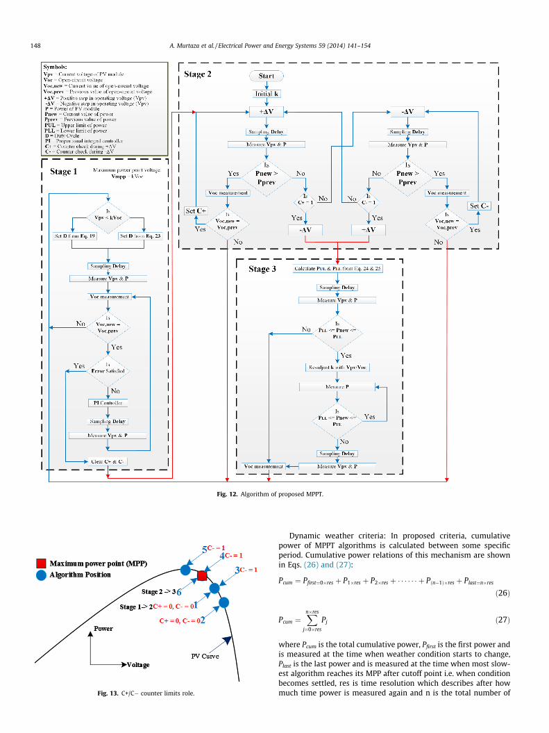
Fig. 12. Algorithm of proposed MPPT.

Fig. 13. C+/C� counter limits role.


Dynamic weather criteria: In proposed criteria, cumulativepower of MPPT algorithms is calculated between some specificperiod. Cumulative power relations of this mechanism are shownin Eqs. (26) and (27):

Pcum ¼ Pfirst¼0�res þ P1�res þ P2�res þ � � � � � � þ Pðn�1Þ�res þ Plast¼n�res

ð26Þ

Pcum ¼Xn�res

j¼0�res

Pj ð27Þ

where Pcum is the total cumulative power, Pfirst is the first power andis measured at the time when weather condition starts to change,Plast is the last power and is measured at the time when most slow-est algorithm reaches its MPP after cutoff point i.e. when conditionbecomes settled, res is time resolution which describes after howmuch time power is measured again and n is the total number of

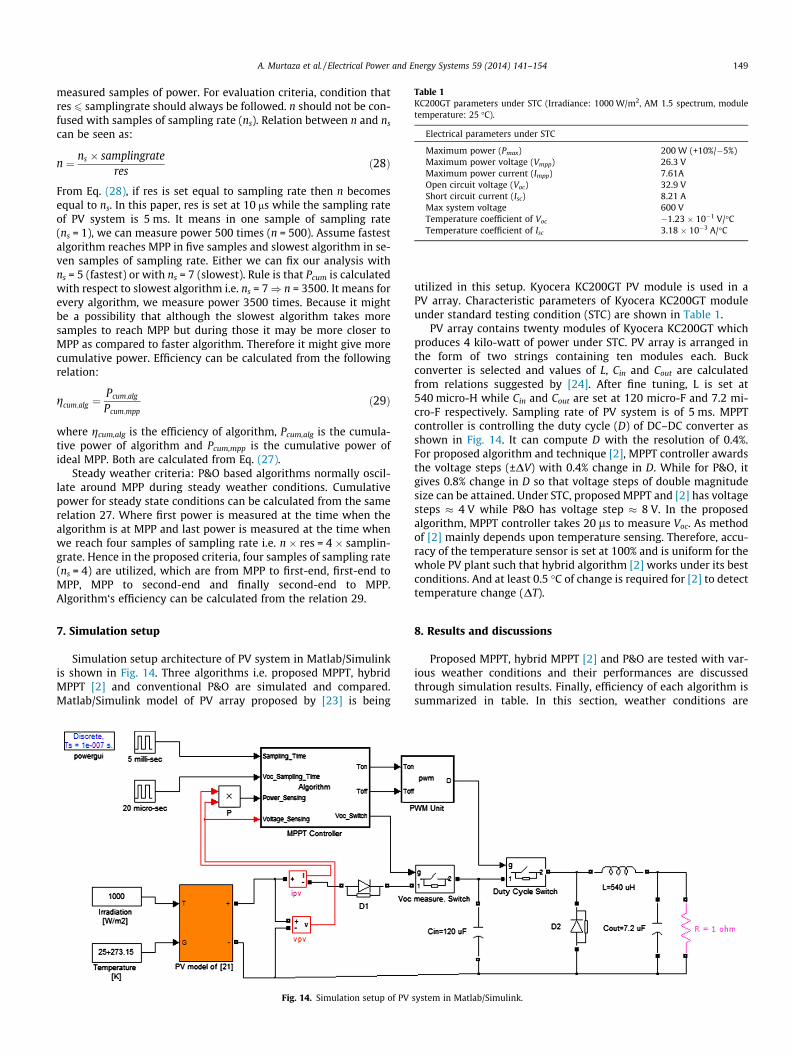
Table 1KC200GT parameters under STC (Irradiance: 1000 W/m2, AM 1.5 spectrum, moduletemperature: 25 �C).

Electrical parameters under STC

Maximum power (Pmax) 200 W (+10%/�5%)Maximum power voltage (Vmpp) 26.3 VMaximum power current (Impp) 7.61AOpen circuit voltage (Voc) 32.9 VShort circuit current (Isc) 8.21 AMax system voltage 600 VTemperature coefficient of Voc �1.23 � 10�1 V/�CTemperature coefficient of Isc 3.18 � 10�3 A/�C


measured samples of power. For evaluation criteria, condition thatres 6 samplingrate should always be followed. n should not be con-fused with samples of sampling rate (ns). Relation between n and ns

can be seen as:

n ¼ ns � samplingrateres

ð28Þ

From Eq. (28), if res is set equal to sampling rate then n becomesequal to ns. In this paper, res is set at 10 ms while the sampling rateof PV system is 5 ms. It means in one sample of sampling rate(ns = 1), we can measure power 500 times (n = 500). Assume fastestalgorithm reaches MPP in five samples and slowest algorithm in se-ven samples of sampling rate. Either we can fix our analysis withns = 5 (fastest) or with ns = 7 (slowest). Rule is that Pcum is calculatedwith respect to slowest algorithm i.e. ns = 7) n = 3500. It means forevery algorithm, we measure power 3500 times. Because it mightbe a possibility that although the slowest algorithm takes moresamples to reach MPP but during those it may be more closer toMPP as compared to faster algorithm. Therefore it might give morecumulative power. Efficiency can be calculated from the followingrelation:

gcum;alg ¼Pcum;alg

Pcum;mppð29Þ

where gcum,alg is the efficiency of algorithm, Pcum,alg is the cumula-tive power of algorithm and Pcum,mpp is the cumulative power ofideal MPP. Both are calculated from Eq. (27).

Steady weather criteria: P&O based algorithms normally oscil-late around MPP during steady weather conditions. Cumulativepower for steady state conditions can be calculated from the samerelation 27. Where first power is measured at the time when thealgorithm is at MPP and last power is measured at the time whenwe reach four samples of sampling rate i.e. n � res = 4 � samplin-grate. Hence in the proposed criteria, four samples of sampling rate(ns = 4) are utilized, which are from MPP to first-end, first-end toMPP, MPP to second-end and finally second-end to MPP.Algorithm‘s efficiency can be calculated from the relation 29.

7. Simulation setup

Simulation setup architecture of PV system in Matlab/Simulinkis shown in Fig. 14. Three algorithms i.e. proposed MPPT, hybridMPPT [2] and conventional P&O are simulated and compared.Matlab/Simulink model of PV array proposed by [23] is being

Fig. 14. Simulation setup of PV

utilized in this setup. Kyocera KC200GT PV module is used in aPV array. Characteristic parameters of Kyocera KC200GT moduleunder standard testing condition (STC) are shown in Table 1.

PV array contains twenty modules of Kyocera KC200GT whichproduces 4 kilo-watt of power under STC. PV array is arranged inthe form of two strings containing ten modules each. Buckconverter is selected and values of L, Cin and Cout are calculatedfrom relations suggested by [24]. After fine tuning, L is set at540 micro-H while Cin and Cout are set at 120 micro-F and 7.2 mi-cro-F respectively. Sampling rate of PV system is of 5 ms. MPPTcontroller is controlling the duty cycle (D) of DC–DC converter asshown in Fig. 14. It can compute D with the resolution of 0.4%.For proposed algorithm and technique [2], MPPT controller awardsthe voltage steps (±DV) with 0.4% change in D. While for P&O, itgives 0.8% change in D so that voltage steps of double magnitudesize can be attained. Under STC, proposed MPPT and [2] has voltagesteps � 4 V while P&O has voltage step � 8 V. In the proposedalgorithm, MPPT controller takes 20 ls to measure Voc. As methodof [2] mainly depends upon temperature sensing. Therefore, accu-racy of the temperature sensor is set at 100% and is uniform for thewhole PV plant such that hybrid algorithm [2] works under its bestconditions. And at least 0.5 �C of change is required for [2] to detecttemperature change (DT).

8. Results and discussions

Proposed MPPT, hybrid MPPT [2] and P&O are tested with var-ious weather conditions and their performances are discussedthrough simulation results. Finally, efficiency of each algorithm issummarized in table. In this section, weather conditions are

system in Matlab/Simulink.


divided into two categories: 1. Dynamic weather conditions and 2.Steady weather conditions.

8.1. Dynamic weather conditions

Dynamic weather conditions mean that at least one factor fromirradiance or temperature should change. It should be noted that

Fig. 15. Response of algorithms und

Fig. 16. Response of techniques und

changeable weather conditions are referenced with the samplingrate. Each sample is of 5 ms. Five cases of dynamic conditions aresimulated.

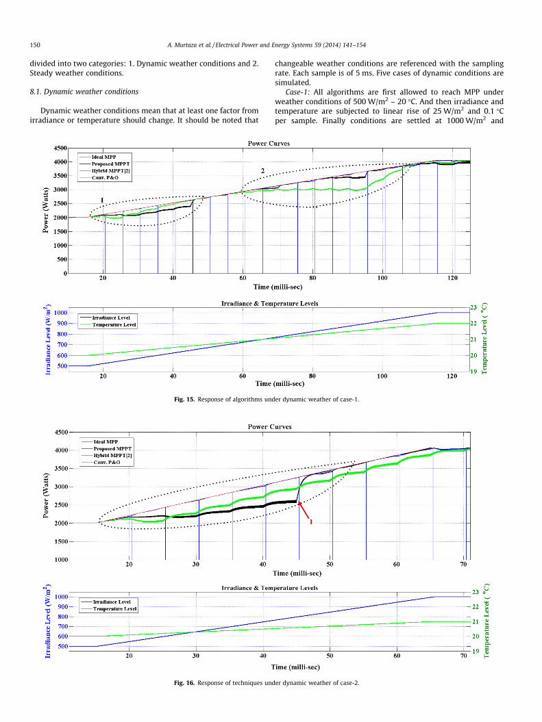
Case-1: All algorithms are first allowed to reach MPP underweather conditions of 500 W/m2 – 20 �C. And then irradiance andtemperature are subjected to linear rise of 25 W/m2 and 0.1 �Cper sample. Finally conditions are settled at 1000 W/m2 and

er dynamic weather of case-1.



22 �C. Response of three algorithms is shown in the upper picturewhile varying weather conditions are indicated in the lowerpicture of Fig. 15. In the lower picture, left vertical axis indicatesirradiance level while the right axis indicates temperature level.It can be seen from Fig. 15 that proposed technique outperforms



others and is very closely following the MPP. From time to time,power curve of proposed technique executes spikes which touchthe horizontal axis indicating the Voc measurements.

It can be seen from dotted area-1 in Fig. 15 that both hybridMPPT [2] and P&O try to reach MPP with their respective voltage




steps. As P&O has a double step size so it has faster convergencespeed as compared to [2]. However technique [2] struggles herebecause during this time, temperature change is less than 0.5 �Cand is not in the detectable range of sensors. Therefore, the tech-nique [2] cannot reset its operating voltage and continues withits P&O. On the other hand, the proposed algorithm performsbetter as it is based on Voc which is measured directly from PVplant. Therefore, it detects the atmosphere in better way. Since athigher irradiance levels the maximum power point voltage virtu-ally remains the same, therefore P&O with its double voltage stepsize struggles more at higher irradiance levels as shown in dottedarea-2 of Fig. 15.

Case 2: This case is same as that of case-1 with the exceptionthat irradiance is changed at much faster rate of 50 W/m2 persample as shown in lower picture of Fig. 16. It can be depicted fromdotted area of Fig. 16 that both hybrid algorithm [2] and P&Ostruggles more with very fast varying irradiance and low tempera-ture change. However proposed technique remains solid andworks better. It should be noted that at arrow-1 position inFig. 16, technique [2] suddenly reached MPP. It is because at thispoint temperature is changed enough for technique [2] to detectit and re-adjusts its operating voltage.

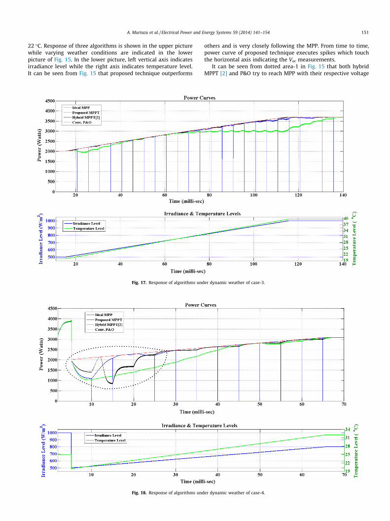
Case 3: In this case, the algorithms are again allowed to settle atMPP under weather conditions of 500 W/m2 – 20 �C. And then

Fig. 19. Response of techniques und

Table 2Summary of dynamic weather cases using evaluation criteria of Section 6.

Cases Variation in weather conditions Efficiency (%) of MPPT algorithms

Irradiance Temperature Proposed MPPT Hybrid MPPT [

1 Medium Low 99.3 97.62 High Low 99.2 93.93 Medium High 99 99.74 High High 95.4 935 Extreme High 90.8 63.2

irradiance and temperature are subjected to linear rise of 25 W/m2 and 1 �C per sample. Finally conditions are settled at 1000 W/m2 and 40 �C. It is clear from Fig. 17 that proposed technique andtechnique [2] are almost performed equally. Performance of tech-nique [2] is enhanced here because of heavy temperature changewhich suits the algorithm’s nature. Proposed algorithm even underthese conditions does not lose its plot and focuses MPP well. How-ever struggle for P&O is still continue.

Case 4: Algorithms are allowed to reach near MPP under1000 W/m2 – 25 �C of weather conditions. Then irradiance andtemperature are subjected to step decay of 500 W/m2 and 20 �Crespectively as shown in Fig. 18. After that weather conditionsare changed up to 800 W/m2 and 32 �C at a linear rise of 25 W/m2 and 1 �C per sample. In this scenario, temperature change is stillheavy but technique [2] is not able to match the proposed method.It is because the sudden decay in irradiance and temperature dis-turbed all three algorithms as indicated by the dotted area inFig. 18. Therefore, there will be significant change in MPP. Pro-posed algorithm works well here because of its D-optimizationmethod which gives the operating voltage a huge boost towardsMPP and then utilizes the PI controller. But, the technique [2]throws its algorithm directly in the hands of PI controller whichtakes more samples to reach MPP. While P&O also gets disturbedand is the slowest one to attain the MPP again.


Performance difference (%) of proposed MPPT to others

2] Conv. P&O Hybrid MPPT [2] Conv. P&O

94.8 +1.7 +4.593.1 +5.3 +6.193 �0.7 +684.4 +2.4 +1180.5 +27.6 +10.3


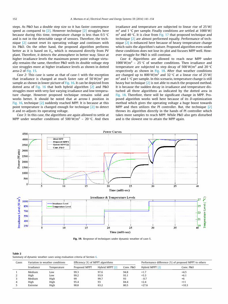
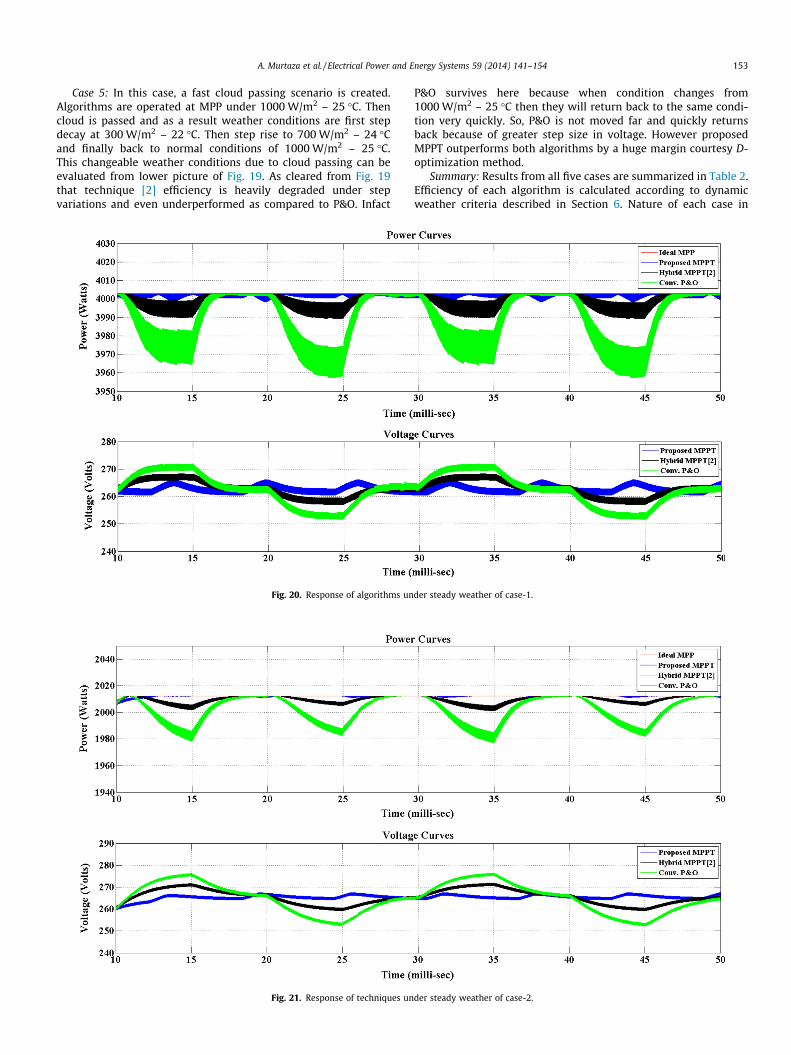
Case 5: In this case, a fast cloud passing scenario is created.Algorithms are operated at MPP under 1000 W/m2 – 25 �C. Thencloud is passed and as a result weather conditions are first stepdecay at 300 W/m2 – 22 �C. Then step rise to 700 W/m2 – 24 �Cand finally back to normal conditions of 1000 W/m2 – 25 �C.This changeable weather conditions due to cloud passing can beevaluated from lower picture of Fig. 19. As cleared from Fig. 19that technique [2] efficiency is heavily degraded under stepvariations and even underperformed as compared to P&O. Infact

Fig. 20. Response of algorithms un

Fig. 21. Response of techniques un

P&O survives here because when condition changes from1000 W/m2 – 25 �C then they will return back to the same condi-tion very quickly. So, P&O is not moved far and quickly returnsback because of greater step size in voltage. However proposedMPPT outperforms both algorithms by a huge margin courtesy D-optimization method.

Summary: Results from all five cases are summarized in Table 2.Efficiency of each algorithm is calculated according to dynamicweather criteria described in Section 6. Nature of each case in

der steady weather of case-1.

der steady weather of case-2.

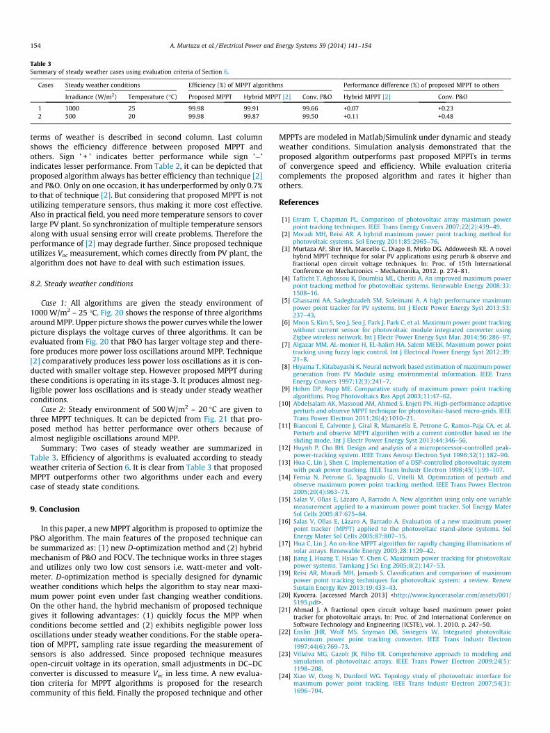
Table 3Summary of steady weather cases using evaluation criteria of Section 6.

Cases Steady weather conditions Efficiency (%) of MPPT algorithms Performance difference (%) of proposed MPPT to others

Irradiance (W/m2) Temperature (�C) Proposed MPPT Hybrid MPPT [2] Conv. P&O Hybrid MPPT [2] Conv. P&O

1 1000 25 99.98 99.91 99.66 +0.07 +0.232 500 20 99.98 99.87 99.50 +0.11 +0.48


terms of weather is described in second column. Last columnshows the efficiency difference between proposed MPPT andothers. Sign ’ + ’ indicates better performance while sign ’�’indicates lesser performance. From Table 2, it can be depicted thatproposed algorithm always has better efficiency than technique [2]and P&O. Only on one occasion, it has underperformed by only 0.7%to that of technique [2]. But considering that proposed MPPT is notutilizing temperature sensors, thus making it more cost effective.Also in practical field, you need more temperature sensors to coverlarge PV plant. So synchronization of multiple temperature sensorsalong with usual sensing error will create problems. Therefore theperformance of [2] may degrade further. Since proposed techniqueutilizes Voc measurement, which comes directly from PV plant, thealgorithm does not have to deal with such estimation issues.

8.2. Steady weather conditions

Case 1: All algorithms are given the steady environment of1000 W/m2 – 25 �C. Fig. 20 shows the response of three algorithmsaround MPP. Upper picture shows the power curves while the lowerpicture displays the voltage curves of three algorithms. It can beevaluated from Fig. 20 that P&O has larger voltage step and there-fore produces more power loss oscillations around MPP. Technique[2] comparatively produces less power loss oscillations as it is con-ducted with smaller voltage step. However proposed MPPT duringthese conditions is operating in its stage-3. It produces almost neg-ligible power loss oscillations and is steady under steady weatherconditions.

Case 2: Steady environment of 500 W/m2 – 20 �C are given tothree MPPT techniques. It can be depicted from Fig. 21 that pro-posed method has better performance over others because ofalmost negligible oscillations around MPP.

Summary: Two cases of steady weather are summarized inTable 3. Efficiency of algorithms is evaluated according to steadyweather criteria of Section 6. It is clear from Table 3 that proposedMPPT outperforms other two algorithms under each and everycase of steady state conditions.

9. Conclusion

In this paper, a new MPPT algorithm is proposed to optimize theP&O algorithm. The main features of the proposed technique canbe summarized as: (1) new D-optimization method and (2) hybridmechanism of P&O and FOCV. The technique works in three stagesand utilizes only two low cost sensors i.e. watt-meter and volt-meter. D-optimization method is specially designed for dynamicweather conditions which helps the algorithm to stay near maxi-mum power point even under fast changing weather conditions.On the other hand, the hybrid mechanism of proposed techniquegives it following advantages: (1) quickly focus the MPP whenconditions become settled and (2) exhibits negligible power lossoscillations under steady weather conditions. For the stable opera-tion of MPPT, sampling rate issue regarding the measurement ofsensors is also addressed. Since proposed technique measuresopen-circuit voltage in its operation, small adjustments in DC–DCconverter is discussed to measure Voc in less time. A new evalua-tion criteria for MPPT algorithms is proposed for the researchcommunity of this field. Finally the proposed technique and other

MPPTs are modeled in Matlab/Simulink under dynamic and steadyweather conditions. Simulation analysis demonstrated that theproposed algorithm outperforms past proposed MPPTs in termsof convergence speed and efficiency. While evaluation criteriacomplements the proposed algorithm and rates it higher thanothers.

References

[1] Esram T, Chapman PL. Comparison of photovoltaic array maximum powerpoint tracking techniques. IEEE Trans Energy Convers 2007;22(2):439–49.

[2] Moradi MH, Reisi AR. A hybrid maximum power point tracking method forphotovoltaic systems. Sol Energy 2011;85:2965–76.

[3] Murtaza AF, Sher HA, Marcello C, Diago B, Mirko DG, Addoweesh KE. A novelhybrid MPPT technique for solar PV applications using perurb & observe andfractional open circuit voltage techniques. In: Proc. of 15th InternationalConference on Mechatronics – Mechatronika, 2012. p. 274–81.

[4] Tafticht T, Agbossou K, Doumbia ML, Cheriti A. An improved maximum powerpoint tracking method for photovoltaic systems. Renewable Energy 2008;33:1508–16.

[5] Ghassami AA, Sadeghzadeh SM, Soleimani A. A high performance maximumpower point tracker for PV systems. Int J Electr Power Energy Syst 2013;53:237–43.

[6] Moon S, Kim S, Seo J, Seo J, Park J, Park C, et al. Maximum power point trackingwithout current sensor for photovoltaic module integrated converter usingZigbee wireless network. Int J Electr Power Energy Syst Mar. 2014;56:286–97.

[7] Algazar MM, AL-monier H, EL-halim HA, Salem MEEK. Maximum power pointtracking using fuzzy logic control. Int J Electrical Power Energy Syst 2012;39:21–8.

[8] Hiyama T, Kitabayashi K. Neural network based estimation of maximum powergeneration from PV Module using environmental information. IEEE TransEnergy Convers 1997;12(3):241–7.

[9] Hohm DP, Ropp ME. Comparative study of maximum power point trackingalgorithms. Prog Photovoltaics Res Appl 2003;11:47–62.

[10] Abdelsalam AK, Massoud AM, Ahmed S, Enjeti PN. High-performance adaptiveperturb and observe MPPT technique for photovoltaic-based micro-grids. IEEETrans Power Electron 2011;26(4):1010–21.

[11] Bianconi E, Calvente J, Giral R, Mamarelis E, Petrone G, Ramos-Paja CA, et al.Perturb and observe MPPT algorithm with a current controller based on thesliding mode. Int J Electr Power Energy Syst 2013;44:346–56.

[12] Huynh P, Cho BH. Design and analysis of a microprocessor-controlled peak-power-tracking system. IEEE Trans Aerosp Electron Syst 1996;32(1):182–90.

[13] Hua C, Lin J, Shen C. Implementation of a DSP-controlled photovoltaic systemwith peak power tracking. IEEE Trans Industr Electron 1998;45(1):99–107.

[14] Femia N, Petrone G, Spagnuolo G, Vitelli M. Optimization of perturb andobserve maximum power point tracking method. IEEE Trans Power Electron2005;20(4):963–73.

[15] Salas V, Olıas E, Lazaro A, Barrado A. New algorithm using only one variablemeasurement applied to a maximum power point tracker. Sol Energy MaterSol Cells 2005;87:675–84.

[16] Salas V, Olıas E, Lazaro A, Barrado A. Evaluation of a new maximum powerpoint tracker (MPPT) applied to the photovoltaic stand-alone systems. SolEnergy Mater Sol Cells 2005;87:807–15.

[17] Hua C, Lin J. An on-line MPPT algorithm for rapidly changing illuminations ofsolar arrays. Renewable Energy 2003;28:1129–42.

[18] Jiang J, Huang T, Hsiao Y, Chen C. Maximum power tracking for photovoltaicpower systems. Tamkang J Sci Eng 2005;8(2):147–53.

[19] Reisi AR, Moradi MH, Jamasb S. Classification and comparison of maximumpower point tracking techniques for photovoltaic system: a review. RenewSustain Energy Rev 2013;19:433–43.

[20] Kyocera. [accessed March 2013] <http://www.kyocerasolar.com/assets/001/5195.pdf>.

[21] Ahmad J. A fractional open circuit voltage based maximum power pointtracker for photovoltaic arrays. In: Proc. of 2nd International Conference onSoftware Technology and Engineering (ICSTE), vol. 1, 2010. p. 247–50.

[22] Enslin JHR, Wolf MS, Snyman DB, Swiegers W. Integrated photovoltaicmaximum power point tracking converter. IEEE Trans Industr Electron1997;44(6):769–73.

[23] Villalva MG, Gazoli JR, Filho ER. Comprehensive approach to modeling andsimulation of photovoltaic arrays. IEEE Trans Power Electron 2009;24(5):1198–208.

[24] Xiao W, Ozog N, Dunford WG. Topology study of photovoltaic interface formaximum power point tracking. IEEE Trans Industr Electron 2007;54(3):1696–704.

http://refhub.elsevier.com/S0142-0615(14)00072-6/h0005

















































http://www.kyocerasolar.com/assets/001/5195.pdf

http://www.kyocerasolar.com/assets/001/5195.pdf










Documents

A duty cycle optimization based hybrid maximum power point tracking technique for photovoltaic systems