A Dynamic Supply-Demand Model for Electricity Prices

Manuela Buzoianu∗, Anthony E. Brockwell, and Duane J. Seppi

Abstract

We introduce a new model for electricity prices, based on the principle of supplyand demand equilibrium. The model includes latent supply and demand curves, whichmay vary over time, and assumes that observed price/quantity pairs are obtained asthe intersection of the two curves, for any particular point in time. Although themodel is highly nonlinear, we explain how the particle filter can be used for modelparameter estimation, and to carry out residual analysis. We apply the model in astudy of Californian wholesale electricity prices over a three-year period including thecrisis period during the year 2000. The residuals indicate that inflated prices do notappear to be attributable to natural random variation, temperature effects, natural gassupply effects, or plant stoppages. However, without ruling out other factors, we areunable to argue whether or not market manipulation by suppliers played a role duringthe crisis period.

1 Introduction

The energy industry provides electrical power to consumers from a variety of sources,including gas-based and hydroelectric plants, as well as nuclear and coal-based power plants.The price of electricity in any given area is governed by complex dynamics, which are drivenby many factors, including, among other things, day-to-day and seasonal variation in de-mand, seasonal variation in temperature, availability of electricity from surrounding regions,and cascade effects when plants are shut down. In addition, major changes can be introducedfor legal reasons, for instance, when deregulation takes place, or when emission permits areissued, etc.

A number of studies have analyzed electricity price time series and market dynamic.Knittel and Roberts (2001) and Deng (2000) attempt to build models that can capturethe volatile behavior of the prices as well as their high jumps. In particular, Knittel andRoberts (2001) emphasize that market models can be improved when the prices are specifiedin relation with exogenous information. In addition, Joskow and Kahn give a nice analysisof the economics of the California market during the crisis of 2000. They explain marketbehavior and its prices by examining a number of factors involved in supply and demand,but do not explicitly pose time series models for the data.

∗Address: Department of Statistics, Carnegie Mellon University, Pittsburgh, PA 15213. E-mail:manuela@stat.cmu.edu.

1

In this paper, we examine the use of a new model, which we refer to as a dynamicsupply-demand model, to simultaneously capture electricity price and usage time series. Thismodel is built on the basic economic principle that on each day, the price and quantity ina competitive market can be determined as the intersection of supply and demand curves.The model incorporates temperature and seasonality effects and gas-availability as factorsby expressing the supply and demand curves as explicit functions of these factors. It alsoallows for intrinsic random variation of the curves over time. Since the model is nonlinearand non-Gaussian, and the supply and demand curves are not directly observable, traditionalmethods for parameter estimation and forecasting are not applicable. However, the particlefiltering algorithm (see,e.g. Salmond and Gordon, 2001; Kitagawa, 1996; Doucet et al., 2001)can be used in this context.

The model is fit to the California electricity market data from April 1998 to December2000. During this time the California market was restructured by divesting part of powerplants to private firms and allowing competition among producers. But it experienced sky-rocketing price values during the second half of 2000, the period often referred to as the“California power crisis”.

The particle filter yields one-step predictive distributions of power prices and quantities.Evaluating predictive cumulative distribution functions at observed data points gives a typeof residual which can be used to evaluate goodness-of-fit. Computing these residuals, we findthat the model fits reasonably well, except that it cannot explain skyrocketing prices duringthe crisis period. Moreover, some of the discrepancies between predicted and observed pricevalues during the crisis are inconsistent with those from the pre-crisis period. One couldargue that this might be due to the so called “perfect storm” conditions, manifested in theform of a dry climate in the Pacific Northwest that reduced hydroelectric power generation,leading to an increase in natural gas prices, and causing demand to exceed supply. However,since our model accounts for most of these factors, the discrepancies suggest that marketstructure may have changed during the second half of 2000. This is of particular interest tothose who would argue that some production firms manipulated the market by withholdingsupply to drive profit margins up.

The paper is organized as follows. In Section 2, we provide a general description of supply-demand pricing principles and introduce our dynamic supply-demand model. In Section 3,we apply the model to analysis of the California energy market, developing specific functionalforms for supply and demand curves, and using a particle-filtering approach to estimate thecurves and obtain residuals. The paper concludes with further brief discussion in Section 4.

2 General Methodology

2.1 Principles of Supply-Demand Pricing

Supply and demand are fundamental concepts of economics. In a competitive market,basic principles of supply and demand determine the price and quantity sold for goods,securities and other tradeable assets. The market for a particular commodity can be regarded

2

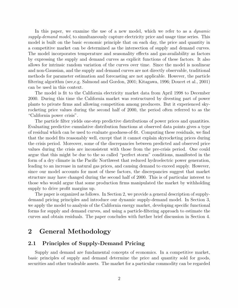
as a collection of entities (individuals or companies) who are willing to buy or sell it. Underthe assumption that the market is competitive, continuous interaction between suppliers anddemanders establishes a unique price for the commodity (see, e.g. Mankiw, 1998).

0 2 4 6 8 100

0.5

1

1.5

2

2.5x 104

SupplyCurve

Price

Quantity Qe

E

DemandCurve

Pe

Figure 1: Typical supply and demand curves. E = (P ε, Qε) is the equilibrium point.

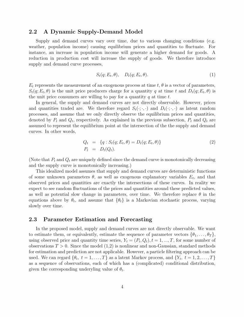
Market supply and demand are established by summing up individual supply and demandschedules. These schedules represent the quantity individuals are willing to trade at any unitprice (see Figure 1-a). The supply curve describes the relationship between the unit price andthe total quantity offered by producers, and is upward-sloping. In the case of electricity, thisupward slope can be explained by the fact that small quantities will be supplied using themost efficient plant available, but that as quantity increases, producers will have to use lessefficient plants, with higher production costs. The demand curve describes the relationshipbetween the unit price and the total quantity desired by consumers. It is downward slopingsince the higher the price, the less people will want to buy (see, e.g. Parkin, 2003). Theintersection of these two curves is the point where supply equals demand, and is called themarket equilibrium (Figure 1-a). This is the point where the price balances supply anddemand schedules. Under the assumption that the market operates efficiently, observedprices will adjust rapidly to this equilibrium point.

When markets are not perfectly competitive, sellers may be able to exercise market powerto maintain prices above equilibrium levels for a significant period of time. In the electricitymarket, this may be possible, due to an oligopolistic structure (e.g. centralized power pools)in which one or few companies have control over production, pricing, distribution etc. Marketpower can also be exercised by suppliers by moving to other markets that pay better, causingthe current market to become less competitive. One way to model this is to factor thesupply curve into two components: a market-free supply component and a “manipulation”component.

3

2.2 A Dynamic Supply-Demand Model

Supply and demand curves vary over time, due to various changing conditions (e.g.weather, population income) causing equilibrium prices and quantities to fluctuate. Forinstance, an increase in population income will generate a higher demand for goods. Areduction in production cost will increase the supply of goods. We therefore introducesupply and demand curve processes,

St(q; Et, θ), Dt(q; Et, θ). (1)

Et represents the measurement of an exogenous process at time t, θ is a vector of parameters,St(q; Et, θ) is the unit price producers charge for a quantity q at time t and Dt(q; Et, θ) isthe unit price consumers are willing to pay for a quantity q at time t.

In general, the supply and demand curves are not directly observable. However, pricesand quantities traded are. We therefore regard St(·; ·, ·) and Dt(·; ·, ·) as latent randomprocesses, and assume that we only directly observe the equilibrium prices and quantities,denoted by Pt and Qt, respectively. As explained in the previous subsection, Pt and Qt areassumed to represent the equilibrium point at the intersection of the the supply and demandcurves. In other words,

Qt = {q : St(q; Et, θ) = Dt(q; Et, θ)} (2)

Pt = Dt(Qt).

(Note that Pt and Qt are uniquely defined since the demand curve is monotonically decreasingand the supply curve is monotonically increasing.)

This idealized model assumes that supply and demand curves are deterministic functionsof some unknown parameters θ, as well as exogenous explanatory variables Et, and thatobserved prices and quantities are exactly the intersections of these curves. In reality weexpect to see random fluctuations of the prices and quantities around these predicted values,as well as potential slow change in parameters, over time. We therefore replace θ in theequations above by θt, and assume that {θt} is a Markovian stochastic process, varyingslowly over time.

2.3 Parameter Estimation and Forecasting

In the proposed model, supply and demand curves are not directly observable. We wantto estimate them, or equivalently, estimate the sequence of parameter vectors {θ1, . . . , θT},using observed price and quantity time series, Yt = (Pt, Qt), t = 1, ..., T , for some number ofobservations T > 0. Since the model (1,2) is nonlinear and non-Gaussian, standard methodsfor estimation and prediction are not applicable. However, a particle filtering approach can beused. We can regard {θt, t = 1, . . . , T} as a latent Markov process, and {Yt, t = 1, 2, . . . , T}as a sequence of observations, each of which has a (complicated) conditional distribution,given the corresponding underyling value of θt.

4

We are particularly interested in obtaining the so-called filtering distributions p(θt|y1, ..., yt),and predictive distributions p(θt|y1, ..., yt−1). These distributions are approximated recur-sively, using the particle filter. The idea is to generate samples {θp,1

t , ..., θp,Nt } and {θf,1

t , ..., θf,Nt },

called ”particles”, which have approximate distributions:

{θp,1t , ..., θ

p,Nt } ∼ p(θt|ys; s = 1, ..., t − 1)

{θf,1t , ..., θ

f,Nt } ∼ p(θt|ys; s = 1, ..., t).

In addition, we will draw (approximate) samples from the the predictive distributions p(yt|ys; s =1, . . . , t − 1).

{y1t , ..., y

Nt } ∼ p(yt|ys; s = 1, ..., t − 1).

N here is a “number of particles”, which can be used to control approximation errors.Larger values of N give smaller approximation errors, but require more computation time.The samples are obtained using the following procedure.

1. Draw θf,j0 ∼ p(θ0), for j = 1, . . . , N

2. Repeat the following steps for t = 1, . . . , T

(a) For j = 1, . . . , N , draw θp,jt from p(θt|θt−1 = θ

f,jt−1).

(b) Compute wjt = p(yt|θt = θ

p,jt ), for j=1,...,N, using the observation equation (2).

(This requires computation of the supply and demand curves corresponding toeach value θ

p,jt , and the intersections of these curves.)

(c) Generate {θf,jt , j = 1, ..., N} by drawing a sample, with replacement, of size N ,

from the set {θp,1t , ..., θ

p,Nt } with probabilities proportional to {wj

t , j = 1, ..., N}.

Step 2(b) requires exogenous information Et to evaluate the required supply and demandcurves. In some cases, when Et is not available at time t, we replace Et in this step with apredictor of Et based on information that is available. We use temperature, for instance, asan exogenous variable, and usually, one day’s temperature is a reasonably good predictor ofthe next day’s temperature. Note also that to implement this procedure the prior p(θ0) andthe transition equation p(θt|θt−1) need to be specified.

At the end of this procedure, we have estimates of the vectors {θt, t = 1, 2, . . . , T},which directly determine our estimates of the supply and demand curves at each time point.As a by-product, we are also able to obtain one-step predictive distributions for the obser-vations, which can be used to compute a “generalized residual”, to be used for diagnosticpurposes. Since the model is nonlinear and non-Gaussian, there is no standard definitionof the residuals, but we can define them using the predictive distribution functions of priceand quantity variables. Specifically, let F P

t (y) denote the one-step empirical predictive cu-mulative distribution function (cdf) for the price Pt, and let F

Qt (y) be the one-step empirical

predictive cdf for the quantity Qt. Then if the model is correct, {F Pt (Pt), t = 1, ..., T}

and {F Qt (Qt), t = 1, ..., T} will form sequences of independent and identically distributed

5

Uniform(0,1) random variables (this follows from results which can be found, among otherplaces, in Rosenblatt, 1952). If desired, these can be converted to Gaussian random vari-ables by applying the inverse standard normal cdf. Thus standard tests can be applied tothe residuals to check for goodness-of-fit.

3 Analysis of Californian Electricity Prices

In this section we apply the techniques described in the previous section in an analysisof Californian electricity prices during the period from April 1st, 1998, to December 31st,2000.

The California energy market underwent a major structural change in April 1998, whenthe electricity generation component was opened to competition with the intent of reducingconsumer prices. The wholesale market, called the “Power Exchange”, was organized as adaily auction. Each day generators and utility companies bid their price and quantity ofenergy, and the Power Exchange calculated a uniform price/quantity pair for all its partici-pants. Utilities were required to satisfy the demand of end-consumers. They also had to sellpower from the stations they owned or controlled through the Power Exchange. A majorcrisis occurred in late 2000, when the utilities were required to purchase power at extremelyhigh prices and sell to end-users at a substantially lower price.

3.1 Data

During 1998-2000, the California Power Exchange operated a day-ahead hour-by-hourauction market. This market ran each day to determine hourly wholesale electricity prices forthe next day. By 7 a.m. each day, generators and retailers submitted a separate schedule ofprice-quantity pairs for each hour of the following day. The Power Exchange assembled theseschedules into demand and supply curves and established the equilibrium point by findingthe intersections of these curves. We focus on this (day-ahead) market since it containsthe majority of trades. Hourly day-ahead market data are available from the University ofCalifornia Energy Institute (http://www.ucei.berkeley.edu/).

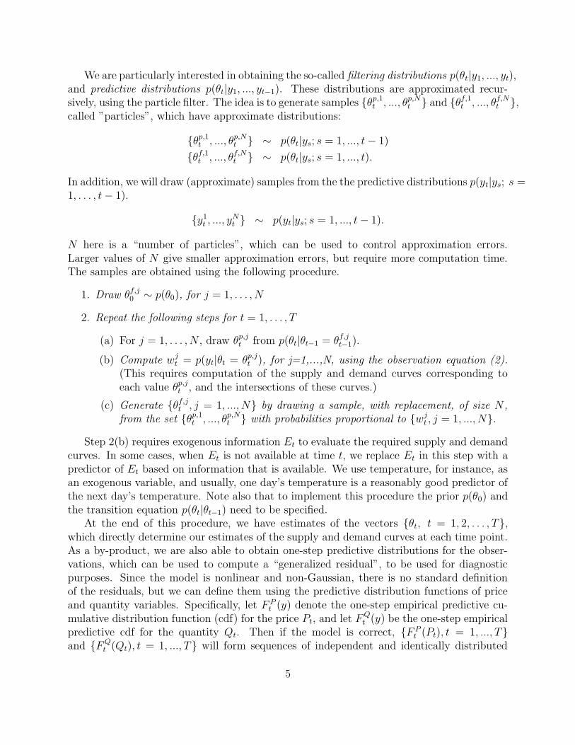
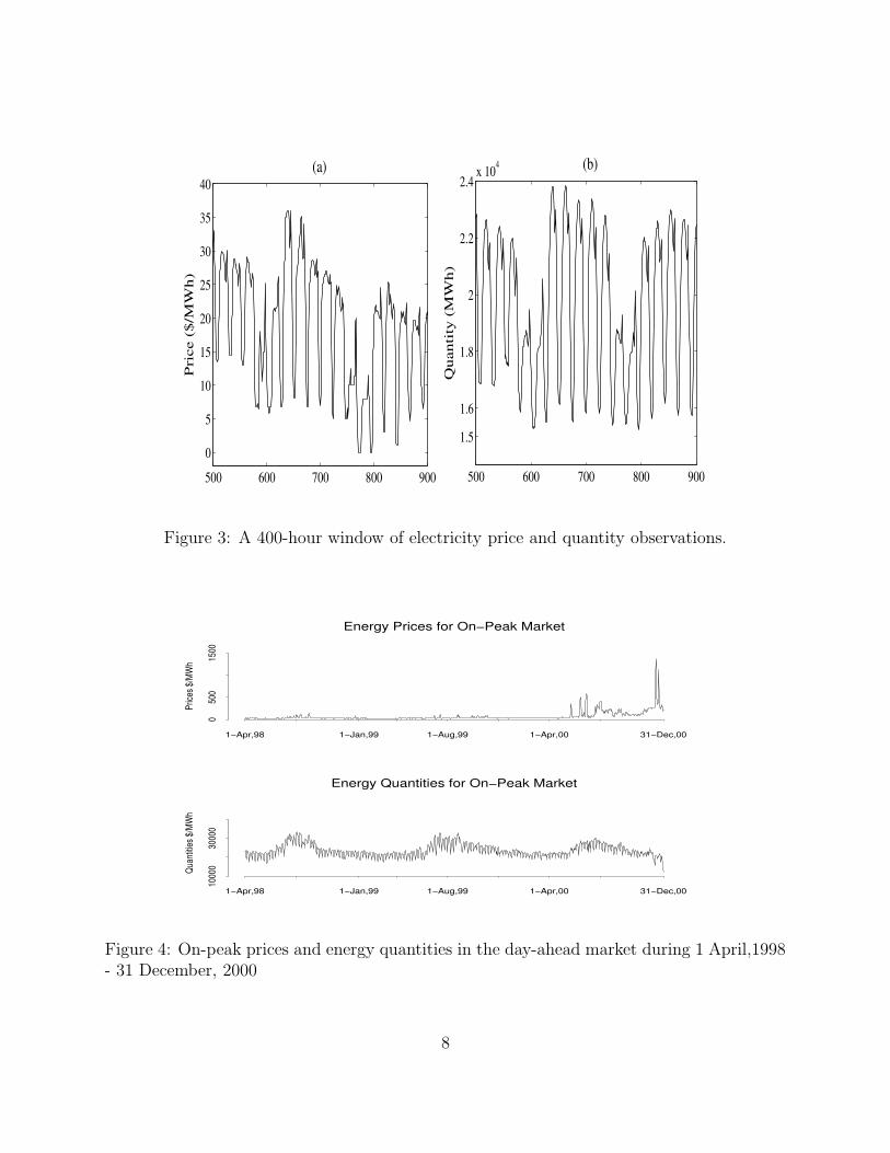
Plots of prices and quantities are given in Figures 2 and 3. They exhibit annual, weekly,and daily seasonal components. The biggest volume of trades of each day are registeredduring the high-demand period from 9 a.m. to 5 p.m. To avoid the need to deal with thedaily cycle, we consider the daily average over the high-demand period. Figure 4 shows theresulting daily prices and quantities. (We will be particularly interested in the large jumpsare registered near the end of the year 2000.)

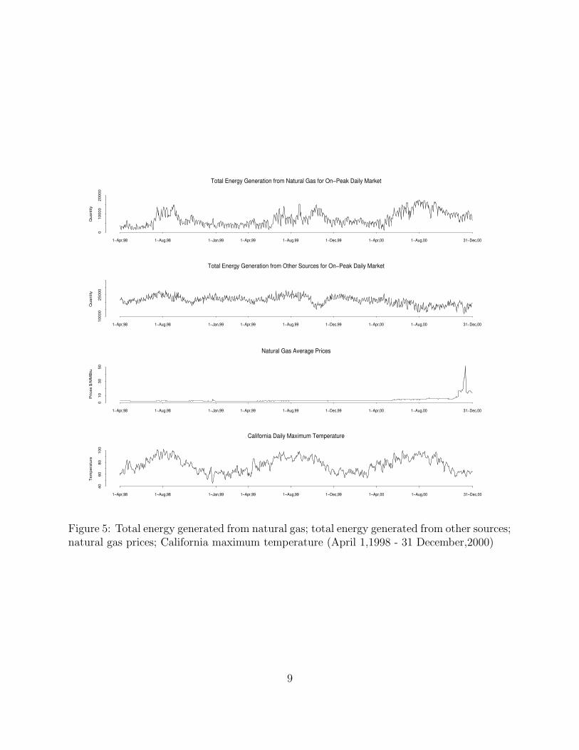
In order to explain prices and quantities, we will use a number of exogenous variables,incorporating them into a particular functional form for the supply and demand curvesSt(·; ·, ·) and Dt(·; ·, ·). These include temperature, natural gas price, quantity of energyproduced from natural gas, and total production of energy. Since daily temperatures areavailable for each California county, we aggregated them to state-wide temperature index bytaking a weighted average based on population weights. Maximum daily temperatures are

6

Price

($/M

Wh)

050

015

00

1a.m./1−Apr,98 1a.m./1−Jan,99 1a.m./1−Aug,99 1a.m./1−Apr,00 12p.m./31−Dec,00

Hourly Day−Ahead Energy PricesQ

uant

ity (M

Wh)

020

000

1a.m./1−Apr,98 1a.m./1−Jan,99 1a.m./1−Aug,99 1a.m./1−Apr,00 12p.m./31−Dec,00

Hourly Day−Ahead Energy Quantities

Figure 2: Hourly prices and quantities in the day-ahead market during April 1, 1998 -December 31, 2000

shown in Figure 5. Natural gas was also an important source of fuel for electricity generationplants in California in 1998-2000, and its availability (or lack thereof) had a significant effecton supply. Power generation based on natural gas accounted for about 75% of the powerproduction private sector, and for about 35% of the total power production. Generatorshad to buy natural gas on the gas market, so gas prices had a direct impact on the powersupply. Natural gas daily prices and the hourly gas based energy quantities are also publiclyavailable, The latter (reduced to daily on-peak data) are shown in Figure 5. Note thatnatural gas prices increased in late 2000, while energy production from natural gas alsoincreased (also Figure 5).

3.2 Specific Form of Supply-Demand Curves

In order to carry out our analysis, we need to determine functional forms for the supplyand demand curves, as a function of parameter vectors θt and also of exogenous variables Et.

7

500 600 700 800 9000

5

10

15

20

25

30

35

40P

rice

($/

MW

h)

500 600 700 800 900

1.5

1.6

1.8

2

2.2

2.4x 104

Qua

ntit

y (M

Wh)

(a) (b)

Figure 3: A 400-hour window of electricity price and quantity observations.

Energy Prices for On−Peak Market

Price

s $/M

Wh

050

015

00

1−Apr,98 1−Jan,99 1−Aug,99 1−Apr,00 31−Dec,00

Energy Quantities for On−Peak Market

Quan

tities

$/MW

h

1000

030

000

1−Apr,98 1−Jan,99 1−Aug,99 1−Apr,00 31−Dec,00

Figure 4: On-peak prices and energy quantities in the day-ahead market during 1 April,1998- 31 December, 2000

8

Total Energy Generation from Natural Gas for On−Peak Daily Market

Qua

ntity

010

000

2000

0

1−Apr,98 1−Aug,98 1−Jan,99 1−Apr,99 1−Aug,99 1−Dec,99 1−Apr,00 1−Aug,00 31−Dec,00

Total Energy Generation from Other Sources for On−Peak Daily Market

Qua

ntity

1000

025

000

1−Apr,98 1−Aug,98 1−Jan,99 1−Apr,99 1−Aug,99 1−Dec,99 1−Apr,00 1−Aug,00 31−Dec,00

Natural Gas Average Prices

Pric

es $

/MM

Btu

010

3050

1−Apr,98 1−Aug,98 1−Jan,99 1−Apr,99 1−Aug,99 1−Dec,99 1−Apr,00 1−Aug,00 31−Dec,00

California Daily Maximum Temperature

Tem

pera

ture

4060

8010

0

1−Apr,98 1−Aug,98 1−Jan,99 1−Apr,99 1−Aug,99 1−Dec,99 1−Apr,00 1−Aug,00 31−Dec,00

Figure 5: Total energy generated from natural gas; total energy generated from other sources;natural gas prices; California maximum temperature (April 1,1998 - 31 December,2000)

9

50 60 70 80 90 100

050

100

150

Maximum Temperature

On−

Pea

k P

rices

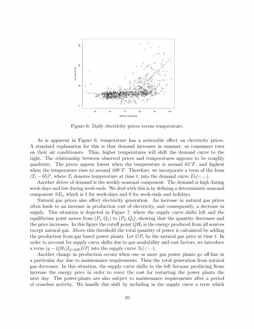
Figure 6: Daily electricity prices versus temperature.

As is apparent in Figure 6, temperature has a noticeable effect on electricity prices.A standard explanation for this is that demand increases in summer, as consumers turnon their air conditioners. Thus, higher temperatures will shift the demand curve to theright. The relationship between observed prices and temperatures appears to be roughlyquadratic. The prices appear lowest when the temperature is around 65◦F , and highestwhen the temperature rises to around 100◦F . Therefore, we incorporate a term of the form(Tt − 65)2, where Tt denotes temperature at time t, into the demand curve Dt(·; ·, ·).

Another driver of demand is the weekly seasonal component. The demand is high duringweek-days and low during week-ends. We deal with this is by defining a deterministic seasonalcomponent SEt, which is 1 for week-days and 0 for week-ends and holidays.

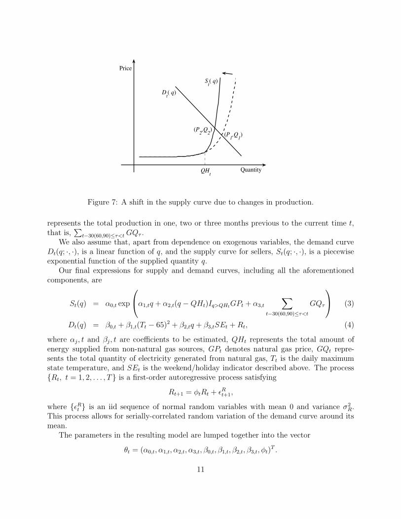
Natural gas prices also affect electricity generation. An increase in natural gas pricesoften leads to an increase in production cost of electricity, and consequently, a decrease insupply. This situation is depicted in Figure 7, where the supply curve shifts left and theequilibrium point moves from (P1, Q1) to (P2, Q2), showing that the quantity decreases andthe price increases. In this figure the cutoff point QHt is the energy produced from all sourcesexcept natural gas. Above this threshold the total quantity of power is calculated by addingthe production from gas based power plants. Let GPt be the natural gas price at time t. Inorder to account for supply curve shifts due to gas availability and cost factors, we introducea term (q − QHt)Iq>QHt

GPt into the supply curve St(·; ·, ·).Another change in production occurs when one or more gas power plants go off-line in

a particular day due to maintenance requirements. Then the total generation from naturalgas decreases. In this situation, the supply curve shifts to the left because producing firmsincrease the energy price in order to cover the cost for restarting the power plants thenext day. The power-plants are also subject to maintenance requirements after a periodof ceaseless activity. We handle this shift by including in the supply curve a term which

10

0 2 4 6 8 100

0.5

1

1.5

2

2.5x 104

St( q)

Price

Quantity QHt

(P1,Q1)(P2,Q2)

Dt( q)

Figure 7: A shift in the supply curve due to changes in production.

represents the total production in one, two or three months previous to the current time t,that is,

∑

t−30(60,90)≤τ<t GQτ .We also assume that, apart from dependence on exogenous variables, the demand curve

Dt(q; ·, ·), is a linear function of q, and the supply curve for sellers, St(q; ·, ·), is a piecewiseexponential function of the supplied quantity q.

Our final expressions for supply and demand curves, including all the aforementionedcomponents, are

St(q) = α0,t exp

α1,tq + α2,t(q − QHt)Iq>QHtGPt + α3,t

∑

t−30(60,90)≤τ<t

GQτ

(3)

Dt(q) = β0,t + β1,t(Tt − 65)2 + β2,tq + β3,tSEt + Rt, (4)

where αj, t and βj, t are coefficients to be estimated, QHt represents the total amount ofenergy supplied from non-natural gas sources, GPt denotes natural gas price, GQt repre-sents the total quantity of electricity generated from natural gas, Tt is the daily maximumstate temperature, and SEt is the weekend/holiday indicator described above. The process{Rt, t = 1, 2, . . . , T} is a first-order autoregressive process satisfying

Rt+1 = φtRt + εRt+1,

where {εRt } is an iid sequence of normal random variables with mean 0 and variance σ2

R.This process allows for serially-correlated random variation of the demand curve around itsmean.

The parameters in the resulting model are lumped together into the vector

θt = (α0,t, α1,t, α2,t, α3,t, β0,t, β1,t, β2,t, β3,t, φt)T .

11

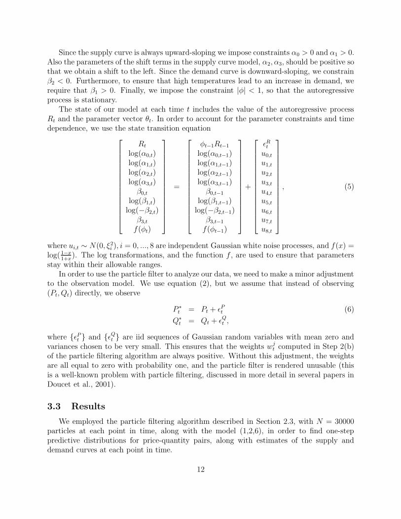
Since the supply curve is always upward-sloping we impose constraints α0 > 0 and α1 > 0.Also the parameters of the shift terms in the supply curve model, α2, α3, should be positive sothat we obtain a shift to the left. Since the demand curve is downward-sloping, we constrainβ2 < 0. Furthermore, to ensure that high temperatures lead to an increase in demand, werequire that β1 > 0. Finally, we impose the constraint |φ| < 1, so that the autoregressiveprocess is stationary.

The state of our model at each time t includes the value of the autoregressive processRt and the parameter vector θt. In order to account for the parameter constraints and timedependence, we use the state transition equation

Rt

log(α0,t)log(α1,t)log(α2,t)log(α3,t)

β0,t

log(β1,t)log(−β2,t)

β3,t

f(φt)

=

φt−1Rt−1

log(α0,t−1)log(α1,t−1)log(α2,t−1)log(α3,t−1)

β0,t−1

log(β1,t−1)log(−β2,t−1)

β3,t−1

f(φt−1)

+

εRt

u0,t

u1,t

u2,t

u3,t

u4,t

u5,t

u6,t

u7,t

u8,t

, (5)

where ui,t ∼ N(0, ξ2i ), i = 0, ..., 8 are independent Gaussian white noise processes, and f(x) =

log(1−x1+x

). The log transformations, and the function f , are used to ensure that parametersstay within their allowable ranges.

In order to use the particle filter to analyze our data, we need to make a minor adjustmentto the observation model. We use equation (2), but we assume that instead of observing(Pt, Qt) directly, we observe

P ∗t = Pt + εP

t (6)

Q∗t = Qt + ε

Qt ,

where {εPt } and {εQ

t } are iid sequences of Gaussian random variables with mean zero andvariances chosen to be very small. This ensures that the weights w

jt computed in Step 2(b)

of the particle filtering algorithm are always positive. Without this adjustment, the weightsare all equal to zero with probability one, and the particle filter is rendered unusable (thisis a well-known problem with particle filtering, discussed in more detail in several papers inDoucet et al., 2001).

3.3 Results

We employed the particle filtering algorithm described in Section 2.3, with N = 30000particles at each point in time, along with the model (1,2,6), in order to find one-steppredictive distributions for price-quantity pairs, along with estimates of the supply anddemand curves at each point in time.

12

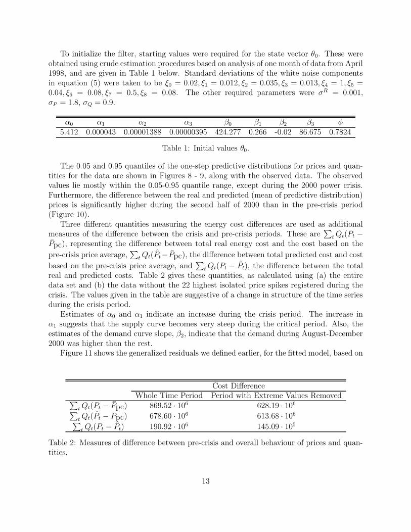
To initialize the filter, starting values were required for the state vector θ0. These wereobtained using crude estimation procedures based on analysis of one month of data from April1998, and are given in Table 1 below. Standard deviations of the white noise componentsin equation (5) were taken to be ξ0 = 0.02, ξ1 = 0.012, ξ2 = 0.035, ξ3 = 0.013, ξ4 = 1, ξ5 =0.04, ξ6 = 0.08, ξ7 = 0.5, ξ8 = 0.08. The other required parameters were σR = 0.001,σP = 1.8, σQ = 0.9.

α0 α1 α2 α3 β0 β1 β2 β3 φ

5.412 0.000043 0.00001388 0.00000395 424.277 0.266 -0.02 86.675 0.7824

Table 1: Initial values θ0.

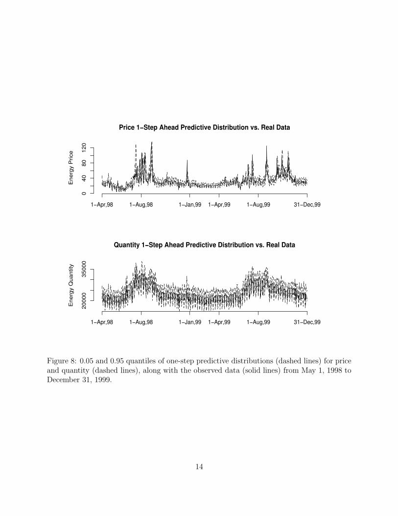
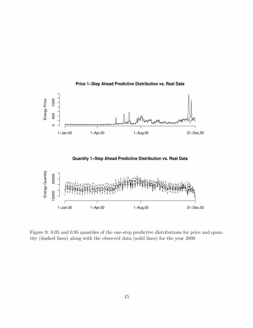
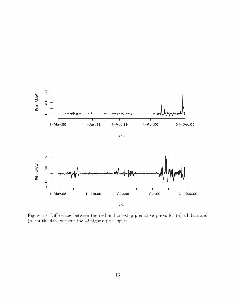
The 0.05 and 0.95 quantiles of the one-step predictive distributions for prices and quan-tities for the data are shown in Figures 8 - 9, along with the observed data. The observedvalues lie mostly within the 0.05-0.95 quantile range, except during the 2000 power crisis.Furthermore, the difference between the real and predicted (mean of predictive distribution)prices is significantly higher during the second half of 2000 than in the pre-crisis period(Figure 10).

Three different quantities measuring the energy cost differences are used as additionalmeasures of the difference between the crisis and pre-crisis periods. These are

∑

t Qt(Pt −P̄pc), representing the difference between total real energy cost and the cost based on the

pre-crisis price average,∑

t Qt(P̂t−P̄pc), the difference between total predicted cost and cost

based on the pre-crisis price average, and∑

t Qt(Pt − P̂t), the difference between the totalreal and predicted costs. Table 2 gives these quantities, as calculated using (a) the entiredata set and (b) the data without the 22 highest isolated price spikes registered during thecrisis. The values given in the table are suggestive of a change in structure of the time seriesduring the crisis period.

Estimates of α0 and α1 indicate an increase during the crisis period. The increase inα1 suggests that the supply curve becomes very steep during the critical period. Also, theestimates of the demand curve slope, β2, indicate that the demand during August-December2000 was higher than the rest.

Figure 11 shows the generalized residuals we defined earlier, for the fitted model, based on

Cost DifferenceWhole Time Period Period with Extreme Values Removed

∑

t Qt(Pt − P̄pc) 869.52 · 106 628.19 · 106

∑

t Qt(P̂t − P̄pc) 678.60 · 106 613.68 · 106

∑

t Qt(Pt − P̂t) 190.92 · 106 145.09 · 105

Table 2: Measures of difference between pre-crisis and overall behaviour of prices and quan-tities.

13

Ener

gy P

rice

Price 1−Step Ahead Predictive Distribution vs. Real Data

040

8012

0

1−Apr,98 1−Aug,98 1−Jan,99 1−Apr,99 1−Aug,99 31−Dec,99

Ener

gy Q

uant

ity

1−Apr,98 1−Aug,98 1−Jan,99 1−Apr,99 1−Aug,99 31−Dec,99

2000

035

000

Quantity 1−Step Ahead Predictive Distribution vs. Real Data

Figure 8: 0.05 and 0.95 quantiles of one-step predictive distributions (dashed lines) for priceand quantity (dashed lines), along with the observed data (solid lines) from May 1, 1998 toDecember 31, 1999.

14

Ener

gy P

rice

Price 1−Step Ahead Predictive Distribution vs. Real Data

1−Jan,00 1−Apr,00 1−Aug,00 31−Dec,00

040

010

00

Ener

gy Q

uant

ity

Quantity 1−Step Ahead Predictive Distribution vs. Real Data

1−Jan,00 1−Apr,00 1−Aug,00 31−Dec,00

1500

030

000

Figure 9: 0.05 and 0.95 quantiles of the one-step predictive distributions for price and quan-tity (dashed lines) along with the observed data (solid lines) for the year 2000

15

Price

$/MW

h

040

080

0

1−May,98 1−Jan,99 1−Aug,99 1−Apr,00 31−Dec,00

(a)

Price

$/MW

h

−100

050

150

1−May,98 1−Jan,99 1−Aug,99 1−Apr,00 31−Dec,00

(b)

Figure 10: Differences between the real and one-step predictive prices for (a) all data and(b) for the data without the 22 highest price spikes.

16

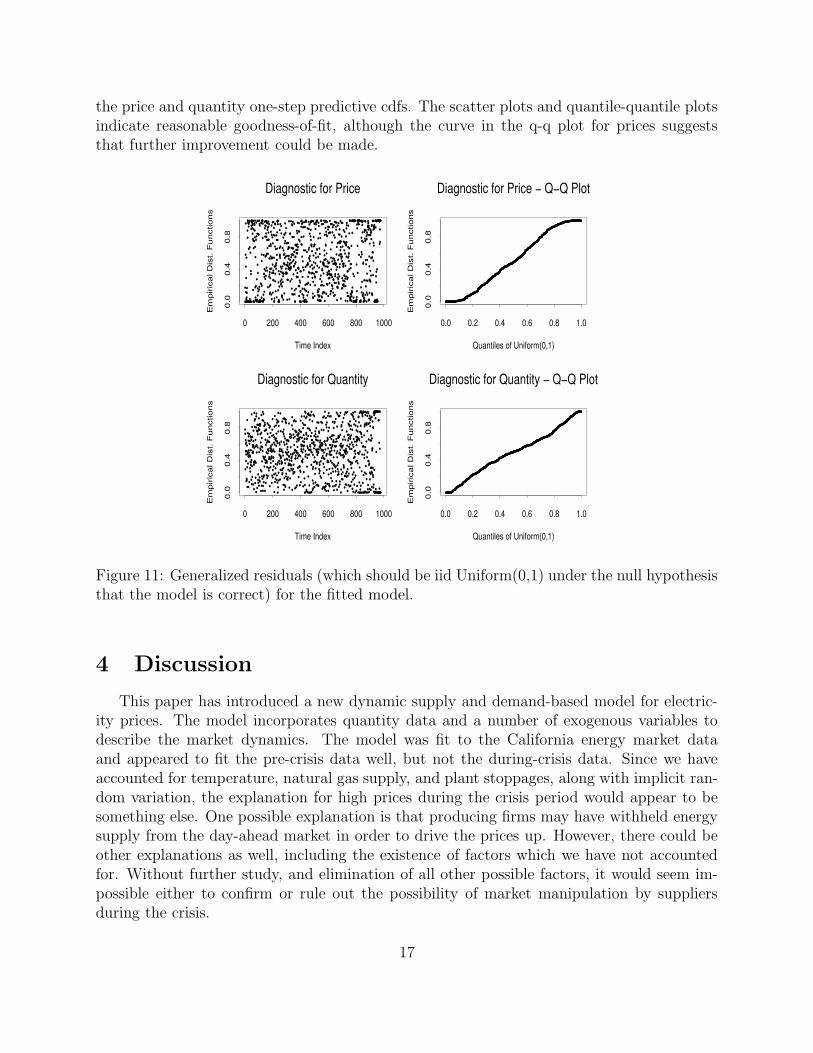
the price and quantity one-step predictive cdfs. The scatter plots and quantile-quantile plotsindicate reasonable goodness-of-fit, although the curve in the q-q plot for prices suggeststhat further improvement could be made.

•••

•

•

•

••

••

•

••••••

•••••

•••

••

•

•••

••

•

••••

•

••

••

•

•••••••••••••

••

•

••

•

•••

•

•••••

•

•

•

•••

•

•

••

•••

•

•

••

•

••

•

•

•

•

••

••••

•

•

••

••••••••

•

•

••

•

••

•

••••••

••••••

•

•

•

•

•••

••••

•

••

••

•

•

•

•

•

••

••

•

•

•

••

•

•••••

•

•

•

••

•••

•

•

•••

••••

•

•

•

••

•

•••

••

•

•

•

•••

••

•

•

•

•••

•

••

•

••

•

•

•

••••

••

•

••••••

•

••

•

•

•

•

•

•

•••••

•

•

•••

•

•

•••••

••

••••••

••

•

•••

•

•

•

••••

•

•

•

••

••

•

•

•

•

•••

•

••

•

•••

•

•

•

•

•••

••

•

••••

•

•

•

••••

•

•

•

•

•••

•

••••

••

•

•

••

•••

•

•

•

•

•••

•

•

•

••

••••

•

•••••

•

•••

•

•

•

•

•

•

•

••

•

•

•

••••

•••

••

•

•

•

••

••

••••

•

••

•••

•

•

•

•••

•

••

•

•••

•

•

•

••

•••••

•

•

••

•

•

•••

••••

••

•••

•

••••••

•

•

•

••••

•

•

•

•••

•

••••••

•

•

••

•

••

•

•••

••••

•

•

•

••

••

•

•

•

•

•••

••

••

••

•••••

•

••

•

•

•••••

•

•

•

••

••

•

•

•••

•

•

•

•

•

••

••

•••

••

•

•••••

•

••

•

•

•••

•

•

•

•••

•

•

•

•

••

••••

••

•

•

•

•

•

••

•••

••

••

•

•••

•

•

•

••

•••

•••

•

••

•

•

•

•••••

•

•

••

•

••

•

•

•

••

•

•

••

•

••

•

•

••

•

••••

••

•

•

•••

•

•

•

•

•••

•

•

•

•

•••

••

•

••

••

••

•

••••

•

•

•

••••

••

•

••

••

•

•

•

••••

••

•

•

••

•

•

••

•••

••

••

•••

•

•

••••

••

•

••

••••

•

•

•

••••

••

•••

••••

•

•

•

•

•

•

•

•••••

•

•

•••••

•

••••

••

•

•

•••••

••••••••••

•

•••

•••

•

•

•••••••••

•

••••••

•••••••

•

•

•••

•

••

•

•••

••

•

•

••

•••••

•

•

••

•

•

•

•

•

•

•

•

•

•••

•

••

••

••

•

••

••••••

•

••

•

••

••

••

•

•

•

•

•

••

•

•

•

•

•

••

••

•

•

•

••

•

•

•

•

•

••

•

•••

••••••

•

•

••

•

•

•

••

••

•

•

•••••

•••••••••••••

•

••••

•••

Diagnostic for Price

Time Index

Em

piric

al D

ist.

Fun

ctio

ns

0 200 400 600 800 1000

0.0

0.4

0.8

•••••••••••••••••••••••••••••••••••••••••••••••••••••••••••••••••••••••••••••••••••••••••••••••••••••••••••••••••••••••••••••••••••••••••••••••••••••••••••••••••••••••••••••••••••••••

•••••••••••••••••••••••••••••••••••••••••••••••••••••••••••••••••••••••••••••••••••••••••••••••••••••••••••••••••

•••••••••••••••••••••••••••••••••••••••••••••••••••••••••••••••••••••••••••••••••••••••••••••••••••••••••••••••••••••••••••••••

•••••••••••••••••••••••••••••••••••••••••••••••••••••••••••••••••••••••••••••••••••••••••••••••••••••

•••••••••••••••••••••••••••••••••••••••••••••••••••••••••••••••••••••••••••••••••••••••••••••••••

•••••••••••••••••••••••••••••••••••••••••••••••••••••••••••••••••••••••••••••••••••••••••••••••••••••••••••••••••••••••••••••••••••••••••••••••••••••••••••••••••••••••••••••••••••••••

Diagnostic for Price − Q−Q Plot

Quantiles of Uniform(0,1)

Em

piric

al D

ist.

Fun

ctio

ns

0.0 0.2 0.4 0.6 0.8 1.0

0.0

0.4

0.8

••

•

••••••

•

•

••

•

•

•

•

••

•

•••

•

••

•••

•

•

••••

•••

•

••••

•

•

•

•

•

•

•

•

•

••••••

•

•••••

•

•

•

•

••

•

•

•

•••

••

•

•

••

•••

•

•

••••••

•••

••••

•

•

•

••

•

•

•

•

••

•

••

•

••

•

••

•

•••

•

•

•

•

••

•

••

••

•

•

•

••

••

•

•

••

•

•

•

•

••

•

•

•

•

••••

•••

•

•

••••

•

•••••••

•

•

•

•••

•

••••••••

•

•

•

•••

••

•••••

••

•

•

•

•

•

••

•

•

•

••••

••••••

••

•

•

•

•

••

•

•

•

•

••

•

•

•

•

••••

•••

•

•

•••

•

•••

••••

••

•

••••

•

•

•

••

•••

•

•

•

•

••

•

•

•

•

•

•

•

•

•

•

••

•••

•

•••

••

••

•

•

••

•

••

•

•

•

••

•

•

•

••

•••

•

•

••

•

•••

•

•

•

••••

•

••

••

••

•

•

••

•

•

••

•

•

••••

•

•

•

•

•

•••

•

•••••••

••••

•

•

•

••

••

••

•

•

•

•

••

•

•

•••••

•

•

•••••

•

•

••

•

•••

•

•

••

•

•

•

••

••

••

•

•

•

•

••

•

•

•

•

•

•••

•

•

•

••

•

•

•

•

•

•

•

•

•

•

•

•

•

•••

•

•

•

••••

•

•

••

•••

•

••••

•

•

•

•

••••

•

•

•

•••

••

•

•

•

•

•••

•

•

••

•••

•

•

•

••••••

•

•

•

•

•

•

•••

••

•••

•

••••

•

•

•

••••

•

•

•••••

•

•

••

•

•

•

•

•

•

••

•

•

•

•

••

••

•

••

•

•

•

••

•

•

•

•

•

•

•

•

•

•

•

••

•

•

•

•

••

•

•

•

••••••

•

••

•••••

•

•

••

•

•

•

••

••

••

••

•

•

•

••

•

•

•

••

••

•

•

•

••

•

•

•

•

•

•

•••

•

••

•

•

•

•

•

••

••••

•

••

••••

•

•

•

•

•

•

••

••

••

••

•

••

••••

•

•••••

•

•

••

••••

•

••

••

•

•

•

••

•

•

••

•

•

•

•

•

•

•

••

••

•••

••

•

••

•••

•

•

•

•

••

•

••

••

••

•

•

•

•

•

•

••

•

••

••

••

••

•••

•

•

•

•

•

••

•

•

•

••••

•

•

•

•••

•

••

•

•

••

••

•

••

•

•

••

•

••

•••

•

•

•

•

•

•

•

•

•

•

•

•••

•

•

•

•

••

••

•

•

•

••

•

•

•

•

•

••

•

•

•

•

•

•

•

•

••

•

•

••

•

•

•

••

•

•

•

•

•

•

•

•

•

•

••

••

••

•

•

•

•

•

••

••

•

•

•

•

•••

•

•••

••

•

•

••

•

•

•••

••

•••

•

•

••

••

•

•

•

••

•••••

••

••

••

•

••

••

•

•

•••

•

•

••••

Diagnostic for Quantity

Time Index

Em

piric

al D

ist.

Fun

ctio

ns

0 200 400 600 800 1000

0.0

0.4

0.8

•••••••••••••••••••••••••••••••••••••••••••••••••••••••••••••••••••••••••••••••••••••••••••••••••••••••••••••••••••••••••••••••••••••••••

•••••••••••••••••••••••••••••••••••••••••••••••••••••••••••••••••••••••••••••••••••••••••••••••••••••••••••••••••••••••••

•••••••••••••••••••••••••••••••••••••••••••••••••••••••••••••••••••••••••••••••••••••••••••••••••••••••••••••••••••••••••••••••••••••••••••••••••••••••••••••••••••••

•••••••••••••••••••••••••••••••••••••••••••••••••••••••••••••••••••••••••••••••••••••••••••••••••••••••••••••••••••••••••••••••••••••••••••••••••••••••••••••••••••••••••••••

•••••••••••••••••••••••••••••••••••••••••••••••••••••••••••••••••••••••••••••••••••••••••••••••••••••••••••••••••••••••••••••••

••••••••••••••••••••••••••••••••••••••••••••••••••••••••••••••••••••••••••••••••••••••••••••••••••

Diagnostic for Quantity − Q−Q Plot

Quantiles of Uniform(0,1)

Em

piric

al D

ist.

Fun

ctio

ns

0.0 0.2 0.4 0.6 0.8 1.0

0.0

0.4

0.8

Figure 11: Generalized residuals (which should be iid Uniform(0,1) under the null hypothesisthat the model is correct) for the fitted model.

4 Discussion

This paper has introduced a new dynamic supply and demand-based model for electric-ity prices. The model incorporates quantity data and a number of exogenous variables todescribe the market dynamics. The model was fit to the California energy market dataand appeared to fit the pre-crisis data well, but not the during-crisis data. Since we haveaccounted for temperature, natural gas supply, and plant stoppages, along with implicit ran-dom variation, the explanation for high prices during the crisis period would appear to besomething else. One possible explanation is that producing firms may have withheld energysupply from the day-ahead market in order to drive the prices up. However, there could beother explanations as well, including the existence of factors which we have not accountedfor. Without further study, and elimination of all other possible factors, it would seem im-possible either to confirm or rule out the possibility of market manipulation by suppliersduring the crisis.

17

References

S. Deng. Pricing electricity derivatives under alternative stochastic spot price models. InProc. of the 33rd Hawaii International Conference on System Sciences, 2000.

A. Doucet, N. de Freitas, and N. Gordon, editors. Sequential Monte Carlo Methods inPractice. Springer, New York, 2001.

P. Joskow and E. Kahn. A quantitative analysis of pricing behavior in california’s wholesaleelectricity markey during summer 2000: The final word. Technical report, MassachusettsInstitute of Technology.

G. Kitagawa. Monte Carlo filter and smoother for non-Gaussian nonlinear state space models.Journal of Computational and Graphical Statistics, 5(1):1–25, 1996.

C.R. Knittel and M.R. Roberts. An empirical examination of deregulated electricity prices.Technical Report PWR-087, Univ. of California Energy Institute, 2001.

G. Mankiw. Principles of Economics. The Dryden Press, 1998.

M. Parkin. Economics. Pearson Eduction, Inc., sixth edition, 2003.

M. Rosenblatt. Remarks on a multivariate transformation. Annals of Mathematical Statistics,23:470–472, 1952.

D. Salmond and N. Gordon. Particles and mixtures for tracking and guidance. In SequentialMonte Carlo Methods in Practice, pages 517–528. Springer, 2001.

18