This content has been downloaded from IOPscience. Please scroll down to see the full text.

Download details:

IP Address: 109.175.147.128

This content was downloaded on 18/05/2014 at 07:00

Please note that terms and conditions apply.

A finite size pencil beam algorithm for IMRT dose optimization: density corrections

View the table of contents for this issue, or go to the journal homepage for more

2007 Phys. Med. Biol. 52 617

(http://iopscience.iop.org/0031-9155/52/3/006)

Home Search Collections Journals About Contact us My IOPscience

INSTITUTE OF PHYSICS PUBLISHING PHYSICS IN MEDICINE AND BIOLOGY

Phys. Med. Biol. 52 (2007) 617–633 doi:10.1088/0031-9155/52/3/006

A finite size pencil beam algorithm for IMRT doseoptimization: density corrections

U Jelen1,2 and M Alber2

1 Faculty of Physics and Applied Computer Science, AGH University of Science andTechnology, Al. Mickiewicza 30, 30-059 Krakow, Poland2 Section for Biomedical Physics, Clinic for Radiooncology, University of Tubingen,Hoppe-Seyler-Str. 3, D-72076 Tubingen, Germany

E-mail: Urszula.Jelen@med.uni-tuebingen.de

Received 23 August 2006, in final form 14 November 2006Published 10 January 2007Online at stacks.iop.org/PMB/52/617

AbstractFor beamlet-based IMRT optimization, fast and less accurate dose computationalgorithms are frequently used, while more accurate algorithms are needed torecompute the final dose for verification. In order to speed up the optimizationprocess and ensure close proximity between dose in optimization andverification, proper consideration of dose gradients and tissue inhomogeneityeffects should be ensured at every stage of the optimization. Due to theirspeed, pencil beam algorithms are often used for precalculation of beamletdose distributions in IMRT treatment planning systems. However, accountingfor tissue heterogeneities with these models requires the use of approximaterescaling methods. Recently, a finite size pencil beam (fsPB) algorithm, basedon a simple and small set of data, was proposed which was specifically designedfor the purpose of dose pre-computation in beamlet-based IMRT. The presentwork describes the incorporation of 3D density corrections, based on MonteCarlo simulations in heterogeneous phantoms, into this method improving thealgorithm accuracy in inhomogeneous geometries while keeping its originalspeed and simplicity of commissioning. The algorithm affords the full accuracyof 3D density corrections at every stage of the optimization, hence providingthe means for density related fluence modulation like penumbra shaping at fieldedges.

(Some figures in this article are in colour only in the electronic version)

1. Introduction

A widely used concept of IMRT treatment planning is based on a decomposition of the broadfield dose distribution into small elements, called beamlets, and requires the pre-computation

0031-9155/07/030617+17$30.00 © 2007 IOP Publishing Ltd Printed in the UK 617

618 U Jelen and M Alber

and storage of the beamlet dose distributions. In the iterative process of optimization, theweights of beamlets are adjusted to satisfy the prescription requirements and eventuallythe dose is re-computed, preferably with a high-precision algorithm (e.g. Monte Carlo).This scheme imposes three main requirements on the dose pre-computation algorithm: (1)speed, due to a large number of beamlet dose distributions to be computed, (2) simplicity ofcommissioning procedure that ideally should be based on broad beam measurements and (3)close proximity between the optimized and the final dose recalculated with a high-precisionalgorithm.

One source of the discrepancies between optimized and recalculated dose is thedifferences between dose computation algorithms in accounting for tissue inhomogeneityeffects. Especially difficult are density heterogeneities like lungs, oral and nasal cavities andpassages, teeth, bones and foreign materials like metal prostheses (AAPM Report 85 (2004))and geometries where the lateral electron equilibrium breaks down.

Various dose calculation algorithms that take inhomogeneities into account have beendeveloped and may be classified according to various criteria (Ahnesjo and Asparadakis 1999,AAPM 2004) depending on the method used to model electron transport, separation of thedose into primary and secondary component or dimensionality of the density information theyuse. The least advanced group of algorithms are correction based methods (e.g. RTAR, Bathomethod (Batho 1964, Sontag and Cunningham 1977) or ETAR (Sontag and Cunningham1978)) that use mass density of the medium to scale the primary fluence, and therefore handlethe scattered component only approximately. They account for the attenuation changes but donot model secondary electron transport and hence overestimate the dose within the low-densityregions and become more inaccurate for higher energies (Arnfield et al 2000, Jones and Das2005, Carrasco et al 2004).

More advanced models, like convolution/superposition (Mackie et al 1985, Boyer andMok 1985, Mohan et al 1986, Ahnesjo 1989), account for tissue density introducing correctionboth for fluence changes and dose spread kernels according to O’Connor’s theorem (O’Connor1957). Kernel scaling (Mackie et al 1985, Mohan et al 1986) allows us to compute the doseaccurately in most instances. However, the strict application of O’Connor’s theorem implies anassumption about the equal atomic composition of media of different densities which ensuresa constant ratio between primary and secondary components of the photon fluence.

Monte Carlo algorithms have the potential to model electron transport in inhomogeneousmedia and have been shown to be the most accurate method for dose computation (Andreo1991, Mohan 1997). However, the computation times are still too long to allow a replacementof the beamlet dose pre-computation engines used in IMRT optimization with Monte Carlo.Attempts have been made to speed up the Monte Carlo computations (Jeraj and Keall 1999)or to use a sequential approach with a fast algorithm to pre-compute the dose and, close toconvergence, continue the optimization with a more accurate algorithm (Laub et al 2000,Siebers et al 2001).

Due to their speed, pencil beam algorithms are commonly used as a pre-calculationdose engine for IMRT treatment planning systems, despite the fact that accounting for tissueheterogeneities with these models is difficult and requires the use of approximate rescaling(Bourland and Chaney 1992) like Batho or EPL methods. Pencil beam based dose computationis especially inaccurate in low-density regions due to the lack of electron transport in the modeland neglection of the lateral electronic disequilibrium (Wang et al 2002).

The impact of simplifications in accounting for tissue inhomogeneities in conventionalradiotherapy was examined by several authors either in anthropomorphic phantoms (Ayyangeret al 1993, Dunscombe et al 1996) or in simplified geometries (Arnfield et al 2000, Carrascoet al 2004, Krieger and Sauer 2005) and suggested to have possible consequences like

A finite size pencil beam algorithm 619

underdosages in nasopharyngeal cases (Martens et al 2002) or small solid tumours locatedwithin the lung tissue and increase of the volume of healthy lung tissue irradiated in thoraxcases (Engelsman et al 2001, Jones and Das 2005). Tests in a real patient geometry describedby du Plessis et al (2001) show inaccuracies of 10–20% for a lung case and 20 up to 70%in a head-and-neck case with nasal sinus included in the radiation field. In case of high-Zmaterials discrepancies between pencil beam and Monte Carlo results in order of 10% of thedose in the target located behind the prosthesis in pelvic irradiation (Laub and Nusslin 2003)and 4–15% in a phantom study (Wieslander and Knoos 2003) were shown.

Although limitations of pencil beam algorithms are well described, their impact oncomplete IMRT treatment plans with specific tumour localizations, sizes and surroundingtissues was not extensively studied and is not well documented (Wang et al 2002). It issupposed that due to combinatorial effects of many small fields and the presence of steepgradients in fields it may be significant, thus a close proximity between the optimized dosedistribution and the final, recalculated dose is crucial for minimization of the convergence error(Laub et al 2000, Jeraj et al 2002, Martens et al 2002) and acceleration of the optimization.

Recently, a finite size pencil beam (fsPB) algorithm, based on a simple and small set ofdata, was proposed which was specifically designed for the purpose of dose pre-computationin beamlet-based IMRT (Jelen et al 2005). The algorithm employs an analytical functionfor the cross-profiles of the beamlets which is based on the assumption of self-consistency,i.e. the requirement that an arbitrary superposition of abutting beamlets should add up toa homogeneous field. The present work describes incorporation of lateral and longitudinaldensity corrections into this method, based on Monte Carlo simulations in heterogeneousphantoms, improving the algorithm accuracy in inhomogeneous geometries while keeping itsoriginal speed and simplicity of commissioning.

2. Methods

Pencil beam algorithms use a pencil kernel which can be understood as a convolution ofsome unit photon fluence (beamlet) of a monodirectional beam with the distribution of energyimparted to the secondary particles by the interacting photon in water. The pencil kernels can bederived from Monte Carlo calculations (Mohan et al 1986, Mackie et al 1988) or from broadbeam measurements by deconvolution (Chui and Mohan 1988) or differentiation (Bortfeldet al 1993, Ceberg et al 1996, Storchi and Woudstra 1996).

2.1. Beamlet dose calculation

In the finite size pencil beam algorithm proposed by Jelen et al (2005), the pencil beamkernel was derived analytically on the basis of the requirement of self-consistency. Thefunction F(x, y,−→w ,−→ux ,−→uy , x0, y0) obtained this way is a weighted sum of two exponentials(equation (1)):

F(x, y,−→w ,−→ux ,−→uy , x0, y0) = w1f (x, y, u1x, u1y, x0, y0) + w2f (x, y, u2x, u2y, x0, y0). (1)

One exponential f (x, y, u2x, u2y, x0, y0) models the primary dose with the penumbra resultingfrom the collimation of primary fluence (source size, shape of leaf ends) and the spread ofelectrons, set in motion by primary photon interactions, at the field edge. The other onef (x, y, u1x, u1y, x0, y0) is much shallower and represents the scattered component of the dose:off-axis head scatter and phantom scatter. Each component is a product of two independentone-dimensional profiles:

f (x, y, uix, uiy, x0, y0) = p(x, uix, x0) · p(y, uiy, y0) (2)

620 U Jelen and M Alber

defined as

p(x, uix, x0) =

sinh(uixx0) exp(uixx) for x < −x0

1 − cosh(uixx) exp(−uixx0) for −x0 � x � x0

sinh(uixx0) exp(−uixx) for x0 < x

. (3)

The full dose distribution of a beamlet derives from a product of a scaling factor A(t, θ)

representing the fluence and the function F(x, y,−→w ,−→ux ,−→uy , x0, y0).

D(�r) = F

(x

ra

,y

ra

,−→w (t),−→ux (t),−→uy (t), x0, y0

)· A(t, θ) ·

(1

ra

)2

, (4)

where �ra denotes projection of �r onto the direction of the beamlet and ra is the length of �ra inunits of the source-to-isocentre distance, x, y are the projections of �r − �ra onto the unit vectorof the x-axis and y-axis of the plane perpendicular to the beamlet direction, t is the geometricaldepth of the point �ra below the patient surface, θ is the angle between the central axis of thebeam and the beamlet.

Steepness parameters of the exponentials (u2x, u2y, u1x, u1y) and weights (w1, w2 =1 −w1) are determined by fitting to cross-profiles of broad square fields modelled with MonteCarlo in a homogeneous waterphantom. Dependences of the parameters u2x, u2y, u1x, u1y, w1

and the scaling factor A(t, θ) on the depth are stored in look-up tables for a set of field sizesand beam energies.

The algorithm constructed in this way allows us to compute the dose in water with anaccuracy of 1–2% and spatial accuracy of penumbra placement of 2 mm for square fields, upto 3 mm for typical irregular IMRT segments.

2.2. Inhomogeneity corrections

The dose deposition in materials different from water is affected by the material densityand composition (atomic number and Z/A ratio). Several authors have shown that doseperturbations induced by inhomogeneities are not linearly dependent on such factors likebeam energy, field size, density and size of the cavity (Li et al 2000, Jones et al 2003) andpostulated that they cannot be described properly by radiological scaling with the mass densityalone. In order to correct for the influence of heterogeneous densities, the parameters of thealgorithm A(t, θ), −→w (t),−→ux (t) and −→uy (t) become dependent on the local density and the trackof the beamlet. Naturally, it is only possible to derive a bulk description of all the physicaleffects involved. In a first step, the density dependence of these parameters was determinedon the basis of Monte Carlo simulations in heterogeneous phantoms.

Doses were computed with the XVMC code with a virtual source model (Fippel 1999,Fippel et al 2003) commissioned for an Elekta Precise linear accelerator (Elekta, Crawley,UK) in a well-chosen phantom geometry. Dose distributions for 20 × 20 cm2 square fieldsfor source–surface distance 90 cm, source–isocentre distance 100 cm and for two energies6 MV and 15 MV were calculated for a homogeneous waterphantom and for a phantom with aslab of different density and 160 mm thickness, inserted at the depth of 80 mm. Slab densitiesranged from 0.1 to 2.0 g cm−3 encompassing the clinically relevant density range from lung3

to bone4. All calculations were performed in a 40 cm × 40 cm × 30 cm waterphantom with(2 mm)3 voxel size and 104 photon histories per cm2 field size.

For all simulated cases, the cross-profiles acquired at various depths were fittedwith a least-squares Levenberg–Marquardt algorithm (Press et al 1992) with a function

3 ρ = 0.25 g cm−3 (AAPM Report 85 (2004)), ρ = 0.26 g cm−3 (ICRU 1992).4 ρ = 1.85 g cm−3 (AAPM Report 85 (2004)), ρ = 1.92 g cm−3 (ICRU 1992).

A finite size pencil beam algorithm 621

6MV 15MV

0 0.2 0.4 0.6 0.8

1 1.2 1.4 1.6 1.8

2

0 50 100 150 200 250 300

A []

depth [mm]

homogeneouswith slab

0 0.2 0.4 0.6 0.8

1 1.2 1.4 1.6 1.8

0 50 100 150 200 250 300

A []

depth [mm]

homogeneouswith slab

0

0.02

0.04

0.06

0.08

0.1

0 50 100 150 200 250 300

u 1 [1

/mm

]

depth [mm]

homogeneouswith slab

0

0.02

0.04

0.06

0.08

0.1

0 50 100 150 200 250 300u 1

[1/m

m]

depth [mm]

homogeneouswith slab

0

0.2

0.4

0.6

0.8

1

0 50 100 150 200 250 300

u 2 [1

/mm

]

depth [mm]

homogeneouswith slab

0

0.2

0.4

0.6

0.8

1

0 50 100 150 200 250 300

u 2 [1

/mm

]

depth [mm]

homogeneouswith slab

0

0.2

0.4

0.6

0.8

1

0 50 100 150 200 250 300

w1

[]

depth [mm]

homogeneouswith slab

0

0.2

0.4

0.6

0.8

1

0 50 100 150 200 250 300

w1

[]

depth [mm]

homogeneouswith slab

0

0.2

0.4

0.6

0.8

1

0 50 100 150 200 250 300

w2

[]

depth [mm]

homogeneouswith slab

0

0.2

0.4

0.6

0.8

1

0 50 100 150 200 250 300

w2

[]

depth [mm]

homogeneouswith slab

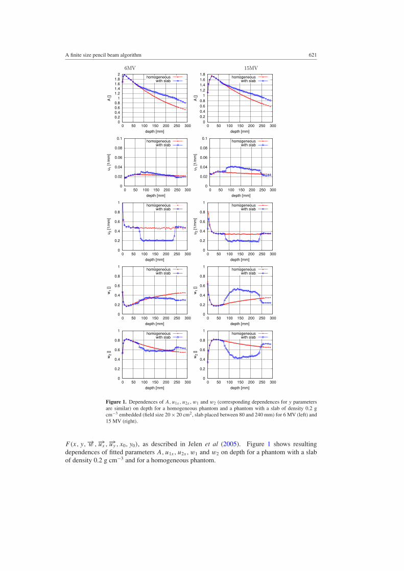
Figure 1. Dependences of A, u1x , u2x , w1 and w2 (corresponding dependences for y parametersare similar) on depth for a homogeneous phantom and a phantom with a slab of density 0.2 gcm−3 embedded (field size 20 × 20 cm2, slab placed between 80 and 240 mm) for 6 MV (left) and15 MV (right).

F(x, y,−→w ,−→ux ,−→uy , x0, y0), as described in Jelen et al (2005). Figure 1 shows resultingdependences of fitted parameters A, u1x, u2x, w1 and w2 on depth for a phantom with a slabof density 0.2 g cm−3 and for a homogeneous phantom.

622 U Jelen and M Alber

In a second step, it was attempted to parametrize the observed behaviour of the fitparameters relative to the values obtained in water. Here, three distinct mechanisms wereidentified as relevant:

(i) a longitudinal correction of primary fluence by an equivalent path length approximation;(ii) penumbra broadening due to an increase in electron range, modelled as a dependency on

the mean local density;(iii) secondary electron disequilibrium, approximated by a dependency on the distance

weighted regional density and a reverse integration over the track of the beamlet.

These approximations aim to mimic the effects of 3D kernel scaling and superposition. Notethat due to the design constraint of self-consistency of the cross-profiles, these correctionsneed not bear an explicit dependency on field size.

2.2.1. Fluence scaling. The primary photon fluence is contained in the scaling factor A(t, θ).Longitudinal scaling of the primary fluence is based on the pathlength scaling concept teq

(equation (5)) (O’Connor 1957, Sontag and Cunningham 1978) and accounts for the variableattenuation along the direction of the beamlet. Equivalent pathlength concept (EPL) allowsus to reconstruct the value of the scaling factor in a heterogeneous medium on the basis ofscaling factor curves obtained in a waterphantom during the commissioning procedure.

teq =∫ t

0

µρ

µH2O· dt ′ =

∫ t

0f (ρ(t ′)) · dt ′, (5)

where teq is the equivalent depth in water, t is the geometrical depth, ρ(t) is the densitydistribution along the beamlet direction, µρ is the total attenuation coefficient in a medium ofdensity ρ, µH2O is the total attenuation coefficient in water.

For derivation of f (ρ), the fit functions based on data from ICRU (1992) (Fippel 1999)were used, that map the mass density onto the linear attenuation coefficients (averaged overthe energy spectrum) for Compton effect and pair production for human tissues and thereforeaccount for the tissue composition.

f6MV(ρ) ={ρ for ρ � ρH2O

0.12 + 0.88 · ρ for ρ > ρH2O(6)

f15MV(ρ) ={ρ for ρ � ρH2O

0.06 + 0.94 · ρ for ρ > ρH2O. (7)

For densities smaller than the density of water, the f (ρ) functions are identical to thewell-established EPL formula; however, the deviation from this formula occurs as a result ofthe decrease of (Z/A) ratio and increase of atomic number of tissues with a density greaterthan water.

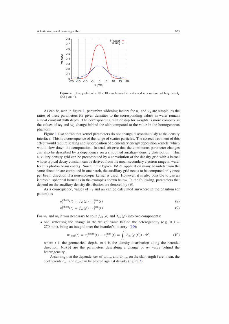
2.2.2. Kernel scaling. The 3D rescaling of the kernel accounts for changes in the rangesand lateral spread of scattered electrons and photons like in the convolution/superpositionmethod. These changes can be described by the appropriate rescaling of the pencil beamkernel parameters acquired in water. The effect of the modification of parameters on the fsPBkernel shape is presented in figure 2.

To adjust the shape of pencil beam profile according to the density, rescaling functionsare introduced, called penumbra widening factors: fu1(ρ), fu2(ρ), fw1(ρ) and fw2(ρ) foru1, u2, w1 and w2, respectively.

A finite size pencil beam algorithm 623

0

0.1

0.2

0.3

0.4

0.5

0.6

0.7

0.8

-20 -15 -10 -5 0 5 10 15 20

rel.d

ose

x [mm]

in waterin lung

Figure 2. Dose profile of a 10 × 10 mm beamlet in water and in a medium of lung density(0.2 g cm−3).

As can be seen in figure 1, penumbra widening factors for u1 and u2 are simple, as theratios of these parameters for given densities to the corresponding values in water remainalmost constant with depth. The corresponding relationship for weights is more complex asthe values of w1 and w2 change behind the slab compared to the value in the homogeneousphantom.

Figure 1 also shows that kernel parameters do not change discontinuously at the densityinterface. This is a consequence of the range of scatter particles. The correct treatment of thiseffect would require scaling and superposition of elementary energy deposition kernels, whichwould slow down the computation. Instead, observe that the continuous parameter changescan also be described by a dependency on a smoothed auxiliary density distribution. Thisauxiliary density grid can be precomputed by a convolution of the density grid with a kernelwhose typical decay constant can be derived from the mean secondary electron range in waterfor this photon beam energy. Since in the typical IMRT application many beamlets from thesame direction are computed in one batch, the auxiliary grid needs to be computed only onceper beam direction if a non-isotropic kernel is used. However, it is also possible to use anisotropic, spherical kernel as in the examples shown below. In the following, parameters thatdepend on the auxiliary density distribution are denoted by (ρ).

As a consequence, values of u1 and u2 can be calculated anywhere in the phantom (orpatient) as

uinhom1 (t) = fu1(ρ) · uhom

1 (t) (8)

uinhom2 (t) = fu2(ρ) · uhom

2 (t). (9)

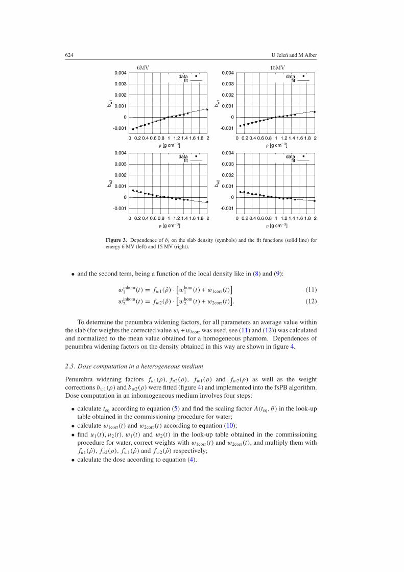
For w1 and w2 it was necessary to split fw1(ρ) and fw2(ρ) into two components:

• one, reflecting the change in the weight value behind the heterogeneity (e.g. at t =270 mm), being an integral over the beamlet’s ‘history’ (10):

wicorr(t) = winhomi (t) − whom

i (t) =∫ t

0bwi(ρ(t ′)) · dt ′, (10)

where t is the geometrical depth, ρ(t) is the density distribution along the beamletdirection, bwi(ρ) are the parameters describing a change of wi value behind theheterogeneity.

Assuming that the dependences of w1corr and w2corr on the slab length l are linear, thecoefficients bw1 and bw2 can be plotted against density (figure 3).

624 U Jelen and M Alber

6MV 15MV

-0.001

0

0.001

0.002

0.003

0.004

0 0.2 0.4 0.6 0.8 1 1.2 1.4 1.6 1.8 2

b w1

ρ [g cm−3]

datafit

-0.001

0

0.001

0.002

0.003

0.004

0 0.2 0.4 0.6 0.8 1 1.2 1.4 1.6 1.8 2

b w1

datafit

-0.001

0

0.001

0.002

0.003

0.004

0 0.2 0.4 0.6 0.8 1 1.2 1.4 1.6 1.8 2

b w2

datafit

-0.001

0

0.001

0.002

0.003

0.004

0 0.2 0.4 0.6 0.8 1 1.2 1.4 1.6 1.8 2b w

2

datafit

ρ [g cm−3] ρ [g cm−3]

ρ [g cm−3]

Figure 3. Dependence of bi on the slab density (symbols) and the fit functions (solid line) forenergy 6 MV (left) and 15 MV (right).

• and the second term, being a function of the local density like in (8) and (9):

winhom1 (t) = fw1(ρ) · [

whom1 (t) + w1corr(t)

](11)

winhom2 (t) = fw2(ρ) · [

whom2 (t) + w2corr(t)

]. (12)

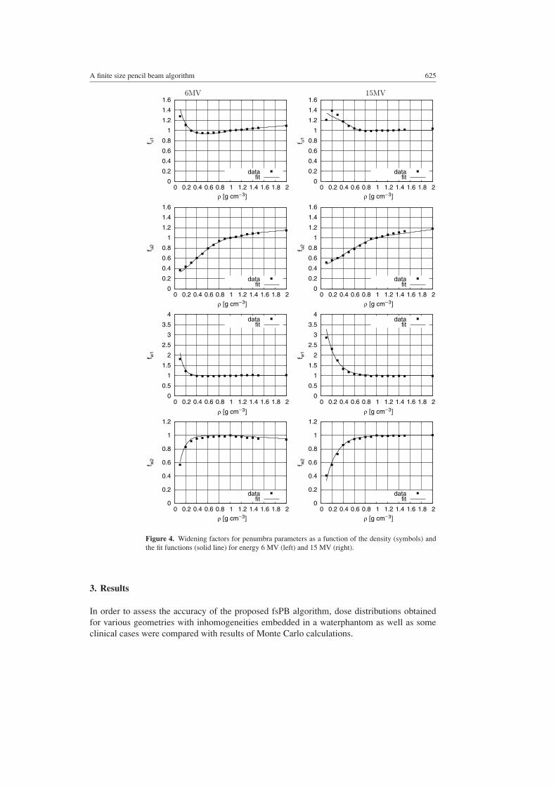
To determine the penumbra widening factors, for all parameters an average value withinthe slab (for weights the corrected value wi +wicorr was used, see (11) and (12)) was calculatedand normalized to the mean value obtained for a homogeneous phantom. Dependences ofpenumbra widening factors on the density obtained in this way are shown in figure 4.

2.3. Dose computation in a heterogeneous medium

Penumbra widening factors fu1(ρ), fu2(ρ), fw1(ρ) and fw2(ρ) as well as the weightcorrections bw1(ρ) and bw2(ρ) were fitted (figure 4) and implemented into the fsPB algorithm.Dose computation in an inhomogeneous medium involves four steps:

• calculate teq according to equation (5) and find the scaling factor A(teq, θ) in the look-uptable obtained in the commissioning procedure for water;

• calculate w1corr(t) and w2corr(t) according to equation (10);• find u1(t), u2(t), w1(t) and w2(t) in the look-up table obtained in the commissioning

procedure for water, correct weights with w1corr(t) and w2corr(t), and multiply them withfu1(ρ), fu2(ρ), fw1(ρ) and fw2(ρ) respectively;

• calculate the dose according to equation (4).

A finite size pencil beam algorithm 625

6MV 15MV

0

0.2

0.4

0.6

0.8

1

1.2

1.4

1.6

0 0.2 0.4 0.6 0.8 1 1.2 1.4 1.6 1.8 2

f u1

datafit

0

0.2

0.4

0.6

0.8

1

1.2

1.4

1.6

0 0.2 0.4 0.6 0.8 1 1.2 1.4 1.6 1.8 2

f u1

datafit

0

0.2

0.4

0.6

0.8

1

1.2

1.4

1.6

0 0.2 0.4 0.6 0.8 1 1.2 1.4 1.6 1.8 2

f u2

datafit

0

0.2

0.4

0.6

0.8

1

1.2

1.4

1.6

0 0.2 0.4 0.6 0.8 1 1.2 1.4 1.6 1.8 2f u

2

datafit

0

0.5

1

1.5

2

2.5

3

3.5

4

0 0.2 0.4 0.6 0.8 1 1.2 1.4 1.6 1.8 2

f w1

datafit

0

0.5

1

1.5

2

2.5

3

3.5

4

0 0.2 0.4 0.6 0.8 1 1.2 1.4 1.6 1.8 2

f w1

datafit

0

0.2

0.4

0.6

0.8

1

1.2

0 0.2 0.4 0.6 0.8 1 1.2 1.4 1.6 1.8 2

f w2

datafit

0

0.2

0.4

0.6

0.8

1

1.2

0 0.2 0.4 0.6 0.8 1 1.2 1.4 1.6 1.8 2

f w2

datafit

ρ [g cm−3] ρ [g cm−3]

ρ [g cm−3]ρ [g cm−3]

ρ [g cm−3] ρ [g cm−3]

ρ [g cm−3]ρ [g cm−3]

Figure 4. Widening factors for penumbra parameters as a function of the density (symbols) andthe fit functions (solid line) for energy 6 MV (left) and 15 MV (right).

3. Results

In order to assess the accuracy of the proposed fsPB algorithm, dose distributions obtainedfor various geometries with inhomogeneities embedded in a waterphantom as well as someclinical cases were compared with results of Monte Carlo calculations.

626 U Jelen and M Alber

6MV 15MV

0

0.5

1

1.5

2

2.5

0 50 100 150 200 250 300

dose

[Gy]

depth [mm]

10x10 —8x8 —6x6 —4x4 —2x2 —

0 0.2 0.4 0.6 0.8

1 1.2 1.4 1.6 1.8

2

0 50 100 150 200 250 300

dose

[Gy]

depth [mm]

10x10 —8x8 —6x6 —4x4 —2x2 —

0

0.5

1

1.5

2

2.5

0 50 100 150 200 250 300

dose

[Gy]

depth [mm]

10x10 —6x6 —4x4 —2x2 —

0 0.2 0.4 0.6 0.8

1 1.2 1.4 1.6 1.8

2

0 50 100 150 200 250 300do

se [G

y]

depth [mm]

10x10 —6x6 —4x4 —2x2 —

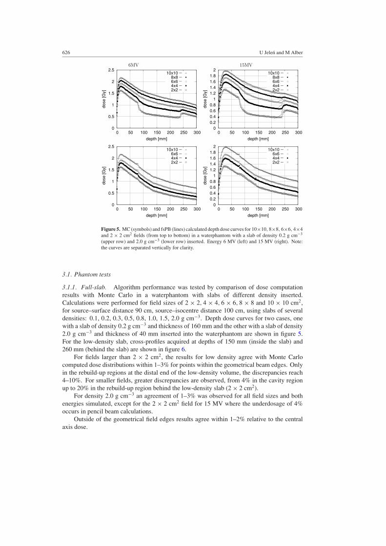
Figure 5. MC (symbols) and fsPB (lines) calculated depth dose curves for 10×10, 8×8, 6×6, 4×4and 2 × 2 cm2 fields (from top to bottom) in a waterphantom with a slab of density 0.2 g cm−3

(upper row) and 2.0 g cm−3 (lower row) inserted. Energy 6 MV (left) and 15 MV (right). Note:the curves are separated vertically for clarity.

3.1. Phantom tests

3.1.1. Full-slab. Algorithm performance was tested by comparison of dose computationresults with Monte Carlo in a waterphantom with slabs of different density inserted.Calculations were performed for field sizes of 2 × 2, 4 × 4, 6 × 6, 8 × 8 and 10 × 10 cm2,for source–surface distance 90 cm, source–isocentre distance 100 cm, using slabs of severaldensities: 0.1, 0.2, 0.3, 0.5, 0.8, 1.0, 1.5, 2.0 g cm−3. Depth dose curves for two cases, onewith a slab of density 0.2 g cm−3 and thickness of 160 mm and the other with a slab of density2.0 g cm−3 and thickness of 40 mm inserted into the waterphantom are shown in figure 5.For the low-density slab, cross-profiles acquired at depths of 150 mm (inside the slab) and260 mm (behind the slab) are shown in figure 6.

For fields larger than 2 × 2 cm2, the results for low density agree with Monte Carlocomputed dose distributions within 1–3% for points within the geometrical beam edges. Onlyin the rebuild-up regions at the distal end of the low-density volume, the discrepancies reach4–10%. For smaller fields, greater discrepancies are observed, from 4% in the cavity regionup to 20% in the rebuild-up region behind the low-density slab (2 × 2 cm2).

For density 2.0 g cm−3 an agreement of 1–3% was observed for all field sizes and bothenergies simulated, except for the 2 × 2 cm2 field for 15 MV where the underdosage of 4%occurs in pencil beam calculations.

Outside of the geometrical field edges results agree within 1–2% relative to the centralaxis dose.

A finite size pencil beam algorithm 627

6MV 15MV

0 0.1 0.2 0.3 0.4 0.5 0.6 0.7 0.8 0.9

1

0 50 100 150 200 250 300

dose

[Gy]

x [mm]

10x10 —8x8 —6x6 —4x4 —2x2 —

0 0.1 0.2 0.3 0.4 0.5 0.6 0.7 0.8 0.9

1

0 50 100 150 200 250 300

dose

[Gy]

x [mm]

10x10 —8x8 —6x6 —4x4 —2x2 —

0

0.1

0.2

0.3

0.4

0.5

0.6

0.7

0.8

0 50 100 150 200 250 300

dose

[Gy]

x [mm]

10x10 —8x8 —6x6 —4x4 —2x2 —

0

0.1

0.2

0.3

0.4

0.5

0.6

0.7

0.8

0 50 100 150 200 250 300do

se [G

y]

x [mm]

10x10 —8x8 —6x6 —4x4 —2x2 —

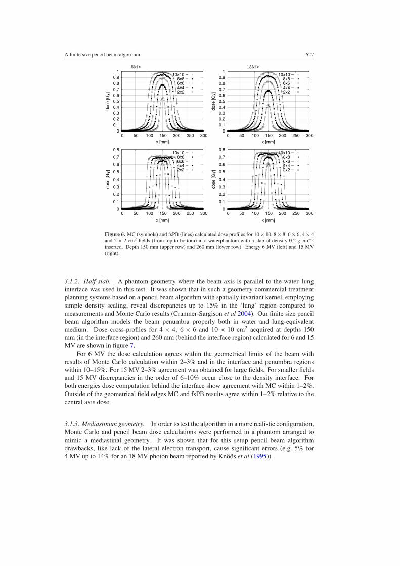
Figure 6. MC (symbols) and fsPB (lines) calculated dose profiles for 10 × 10, 8 × 8, 6 × 6, 4 × 4and 2 × 2 cm2 fields (from top to bottom) in a waterphantom with a slab of density 0.2 g cm−3

inserted. Depth 150 mm (upper row) and 260 mm (lower row). Energy 6 MV (left) and 15 MV(right).

3.1.2. Half-slab. A phantom geometry where the beam axis is parallel to the water–lunginterface was used in this test. It was shown that in such a geometry commercial treatmentplanning systems based on a pencil beam algorithm with spatially invariant kernel, employingsimple density scaling, reveal discrepancies up to 15% in the ‘lung’ region compared tomeasurements and Monte Carlo results (Cranmer-Sargison et al 2004). Our finite size pencilbeam algorithm models the beam penumbra properly both in water and lung-equivalentmedium. Dose cross-profiles for 4 × 4, 6 × 6 and 10 × 10 cm2 acquired at depths 150mm (in the interface region) and 260 mm (behind the interface region) calculated for 6 and 15MV are shown in figure 7.

For 6 MV the dose calculation agrees within the geometrical limits of the beam withresults of Monte Carlo calculation within 2–3% and in the interface and penumbra regionswithin 10–15%. For 15 MV 2–3% agreement was obtained for large fields. For smaller fieldsand 15 MV discrepancies in the order of 6–10% occur close to the density interface. Forboth energies dose computation behind the interface show agreement with MC within 1–2%.Outside of the geometrical field edges MC and fsPB results agree within 1–2% relative to thecentral axis dose.

3.1.3. Mediastinum geometry. In order to test the algorithm in a more realistic configuration,Monte Carlo and pencil beam dose calculations were performed in a phantom arranged tomimic a mediastinal geometry. It was shown that for this setup pencil beam algorithmdrawbacks, like lack of the lateral electron transport, cause significant errors (e.g. 5% for4 MV up to 14% for an 18 MV photon beam reported by Knoos et al (1995)).

628 U Jelen and M Alber

6MV 15MV

0

0.2

0.4

0.6

0.8

1

1.2

0 50 100 150 200 250 300

dose

[Gy]

x [mm]

10x10 —6x6 —4x4 —2x2 —

0

0.2

0.4

0.6

0.8

1

1.2

0 50 100 150 200 250 300

dose

[Gy]

x [mm]

10x10 —6x6 —4x4 —2x2 —

0

0.1

0.2

0.3

0.4

0.5

0.6

0.7

0.8

0 50 100 150 200 250 300

dose

[Gy]

x [mm]

10x10 —6x6 —4x4 —2x2 —

0

0.1

0.2

0.3

0.4

0.5

0.6

0.7

0.8

0 50 100 150 200 250 300do

se [G

y]

x [mm]

10x10 —6x6 —4x4 —2x2 —

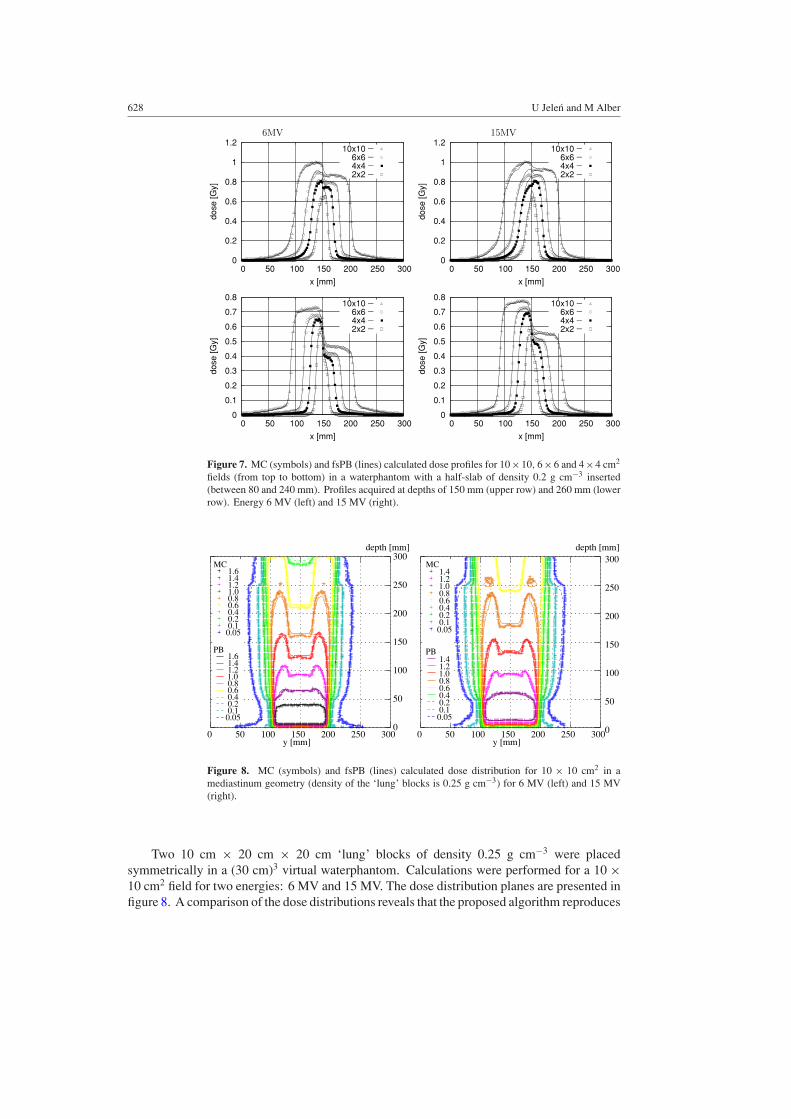
Figure 7. MC (symbols) and fsPB (lines) calculated dose profiles for 10×10, 6×6 and 4×4 cm2

fields (from top to bottom) in a waterphantom with a half-slab of density 0.2 g cm−3 inserted(between 80 and 240 mm). Profiles acquired at depths of 150 mm (upper row) and 260 mm (lowerrow). Energy 6 MV (left) and 15 MV (right).

300

250

200

150

100

50

0 100 150 200 250 300 500

depth [mm]

y [mm]

1.6 1.4 1.2

0.8 0.6 0.4 0.2 0.1 0.05

1.0

1.4 1.2

0.8 0.6 0.4 0.2 0.1 0.05

1.6

1.0

MC

PB

300

250

200

150

100

50

0

depth [mm]

150 200 250 300 100 500y [mm]

1.4 1.2

0.8 0.6 0.4 0.2 0.1 0.05

1.0

1.4 1.2

0.8 0.6 0.4 0.2 0.1 0.05

1.0

MC

PB

Figure 8. MC (symbols) and fsPB (lines) calculated dose distribution for 10 × 10 cm2 in amediastinum geometry (density of the ‘lung’ blocks is 0.25 g cm−3) for 6 MV (left) and 15 MV(right).

Two 10 cm × 20 cm × 20 cm ‘lung’ blocks of density 0.25 g cm−3 were placedsymmetrically in a (30 cm)3 virtual waterphantom. Calculations were performed for a 10 ×10 cm2 field for two energies: 6 MV and 15 MV. The dose distribution planes are presented infigure 8. A comparison of the dose distributions reveals that the proposed algorithm reproduces

A finite size pencil beam algorithm 629

(A)

(C)

(B)

(D)

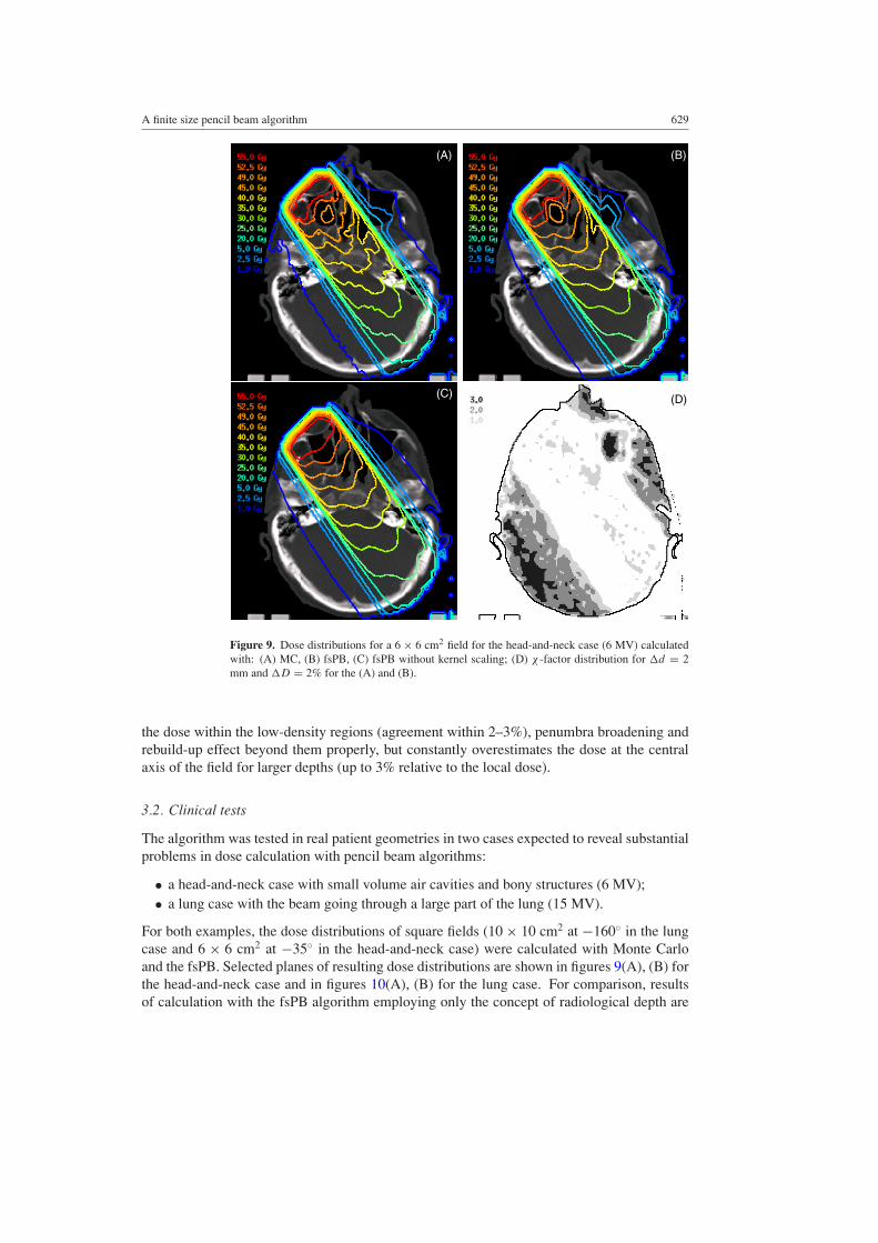
Figure 9. Dose distributions for a 6 × 6 cm2 field for the head-and-neck case (6 MV) calculatedwith: (A) MC, (B) fsPB, (C) fsPB without kernel scaling; (D) χ -factor distribution for �d = 2mm and �D = 2% for the (A) and (B).

the dose within the low-density regions (agreement within 2–3%), penumbra broadening andrebuild-up effect beyond them properly, but constantly overestimates the dose at the centralaxis of the field for larger depths (up to 3% relative to the local dose).

3.2. Clinical tests

The algorithm was tested in real patient geometries in two cases expected to reveal substantialproblems in dose calculation with pencil beam algorithms:

• a head-and-neck case with small volume air cavities and bony structures (6 MV);• a lung case with the beam going through a large part of the lung (15 MV).

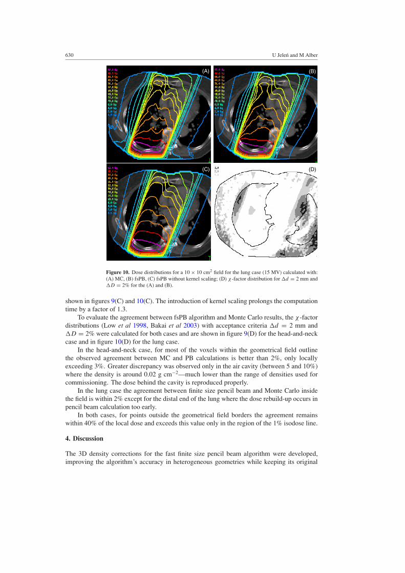
For both examples, the dose distributions of square fields (10 × 10 cm2 at −160◦ in the lungcase and 6 × 6 cm2 at −35◦ in the head-and-neck case) were calculated with Monte Carloand the fsPB. Selected planes of resulting dose distributions are shown in figures 9(A), (B) forthe head-and-neck case and in figures 10(A), (B) for the lung case. For comparison, resultsof calculation with the fsPB algorithm employing only the concept of radiological depth are

630 U Jelen and M Alber

(A) (B)

(C) (D)

Figure 10. Dose distributions for a 10 × 10 cm2 field for the lung case (15 MV) calculated with:(A) MC, (B) fsPB, (C) fsPB without kernel scaling; (D) χ -factor distribution for �d = 2 mm and�D = 2% for the (A) and (B).

shown in figures 9(C) and 10(C). The introduction of kernel scaling prolongs the computationtime by a factor of 1.3.

To evaluate the agreement between fsPB algorithm and Monte Carlo results, the χ -factordistributions (Low et al 1998, Bakai et al 2003) with acceptance criteria �d = 2 mm and�D = 2% were calculated for both cases and are shown in figure 9(D) for the head-and-neckcase and in figure 10(D) for the lung case.

In the head-and-neck case, for most of the voxels within the geometrical field outlinethe observed agreement between MC and PB calculations is better than 2%, only locallyexceeding 3%. Greater discrepancy was observed only in the air cavity (between 5 and 10%)where the density is around 0.02 g cm−2—much lower than the range of densities used forcommissioning. The dose behind the cavity is reproduced properly.

In the lung case the agreement between finite size pencil beam and Monte Carlo insidethe field is within 2% except for the distal end of the lung where the dose rebuild-up occurs inpencil beam calculation too early.

In both cases, for points outside the geometrical field borders the agreement remainswithin 40% of the local dose and exceeds this value only in the region of the 1% isodose line.

4. Discussion

The 3D density corrections for the fast finite size pencil beam algorithm were developed,improving the algorithm’s accuracy in heterogeneous geometries while keeping its original

A finite size pencil beam algorithm 631

speed and simplicity of commissioning. The approach preserves the self-consistency of theprofiles, which is a necessary condition even in heterogeneous media due to linearity betweenprimary fluence and dose.

The correction factors extracted form the Monte Carlo simulated data are an approximationof the bulk effects, like the penumbra broadening and the dose drop in the low-density regions,that occur due to density changes. Penumbra widening factors, introduced to rescale the kernel,model the influence of the tissue composition and density on the secondary particle transportand their behaviour, are consistent with expectations. The shape of the primary penumbrawidening factor fu2(ρ) obtained in the commissioning procedure corresponds to an inverseproportionality between the penumbra width and density, that was observed experimentallyby Hoban et al (1992). As the primary penumbra represents the spread of Compton electrons,this character of the curve is a consequence of an inverse dependence between the range ofelectrons and the density. A weaker, but similar dependence was expected for the secondarypenumbra correction factor fu1(ρ). However, disequilibrium effects, when the width of thepenumbral region becomes comparable to the field dimensions, misguide the fitting procedureresulting in a seemingly steeper penumbra (larger u1) that is compensated by larger w1 andsmaller w2 (figure 4) for low-density media.

A set of phantom tests in heterogeneous geometries was performed in order to evaluatethe accuracy of the proposed algorithm. An overall agreement in the order of 3%/3 mmwas observed, fulfilling the criteria proposed by Venselaar et al (2001) for dose calculationin heterogeneous media. Larger discrepancies (10–15%) were observed at extreme densityinterfaces. The overestimation of the dose in this region is a consequence of the omission ofthe non-isotropic components of the electron kernel. This effect, however, will be significantlyreduced in the patient geometry, where the edges between regions of different densities aresmoother than in the phantom models.

The inclusion of lateral and longitudinal density corrections into an fsPB algorithmimproved its agreement with Monte Carlo computations thereby ensuring a close proximityof the dose distribution between optimization and verification.

Acknowledgments

This work was supported by DFG grant Nu 33/7-2 and Computerized Medical Systems(CMS).

References

Ahnesjo A and Asparadakis M M 1999 Dose calculations for external photon beams in radiotherapy Phys. Med.Biol. 44 R99–155

Ahnesjo A 1989 Collapsed cone convolution of radiant energy for photon dose calculation in heterogeneous mediaMed. Phys. 16 577–92

AAPM 2004 Tissue inhomogeneity corrections for megavoltage photon beams AAPM Report 85 Report of TaskGroup No. 65 of the Radiation Therapy Committee of the American Association of Physicists in Medicine(Madison, WI: Medical Physics Publishing)

Andreo P 1991 Monte Carlo techniques in medical radiation physics Phys. Med. Biol. 36 861–920Arnfield M R, Siantar C H, Siebers J, Garmon P, Cox L and Mohan R 2000 The impact of electron transport on the

accuracy of computed dose Med. Phys. 27 1266–74Ayyangar K, Palta J R, Sweet J W and Suntharalingam N 1993 Experimental verification of a three-dimensional dose

calculation algorithm using a specially designed heterogeneous phantom Med. Phys. 20 325–9Bakai A, Alber M and Nusslin F 2003 A revision of the γ -evaluation concept for the comparison of dose distributions

Phys. Med. Biol. 48 3543–53Batho H F 1964 Lung corrections in cobalt 60 beam therapy J. Can. Assoc. Radiol. 15 79–83

632 U Jelen and M Alber

Bortfeld T, Schlegel W and Rhein B 1993 Decomposition of pencil beam kernels for fast dose calculation in three-dimensional treatment planning Med. Phys. 20 311–18

Bourland J D and Chaney E L 1992 A finite-size pencil beam model for photon dose calculations in three dimensionsMed. Phys. 19 1401–12

Boyer A and Mok E 1985 A photon dose distribution model employing convolution calculations Med. Phys. 12 169–77Carrasco P, Jornet N, Duch M A, Weber L, Ginjaume M, Eudaldo T, Jurado D, Ruiz A and Ribas M 2004 Comparison

of dose calculation algorithms in phantoms with lung equivalent heterogeneities under conditions of lateralelectronic disequilibrium Med. Phys. 31 2889–911

Ceberg C P, Bjarngard B E and Zhu T C 1996 Experimental determination of the dose kernel in high-energy x-raybeams Med. Phys. 23 505–11

Cranmer-Sargison G, Beckham W A and Popescu I A 2004 Modelling an extreme water–lung interface using a singlepencil beam algorithm and the Monte Carlo method Phys. Med. Biol. 49 1557–67

Chui C-S and Mohan R 1988 Extraction of pencil beam kernels by the deconvolution method Med. Phys. 15 138–44Dunscombe P, McGhee P and Lederer E 1996 Anthropomorphic phantom measurements for the validation of a

treatment planning system Phys. Med. Biol. 41 399–411Engelsman M, Damen E M F, Koken P W, van ’t Veld A A, van Ingen K M and Mijnheer B J 2001 Impact

of simple tissue inhomogeneity correction algorithms on conformal radiotherapy of lung tumours Radiother.Oncol. 60 299–309

Fippel M 1999 Fast Monte Carlo dose calculation for photon beams based on the VMC electron algorithm Med.Phys 26 1466–75

Fippel M, Haryanto F, Dohm O, Nusslin F and Kriesen S 2003 A virtual photon energy fluence model for MonteCarlo dose calculation Med. Phys. 30 301–11

Hoban P W, Keal P J and Round W H 1992 The effect of density on the 10 MV photon beam penumbra Australas.Phys. Eng. Sci. Med. 15 113–23

ICRU 1992 Photon, electron, proton and neutron interaction data for body tissues ICRU Report 46 (Bethesda, MD:International Commission on Radiation Units and Measurements)

Jelen U, Sohn M and Alber M 2005 A finite size pencil beam for IMRT dose optimization Phys. Med. Biol. 50 1747–66Jeraj R and Keall P J 1999 Monte Carlo-based inverse treatment planning Phys. Med. Biol. 44 1885–96Jeraj R, Keall P J and Siebers J V 2002 The effect of dose calculation accuracy on inverse treatment planning Phys.

Med. Biol. 47 391–407Jones A O and Das I J 2005 Comparison of inhomogeneity correction algorithms in small photon fields Med.

Phys. 32 766–76Jones A O, Das I J and Jones F L Jr 2003 A Monte Carlo study of IMRT beamlets in inhomogeneous media Med.

Phys. 30 296–300Knoos T, Ahnesjo A, Nilsson P and Weber L 1995 Limitations of a pencil beam approach to photon dose calculations

in lung tissue Phys. Med. Biol. 40 1411–20Krieger T and Sauer O A 2005 Monte Carlo- versus pencil-beam-/collapsed-cone- dose calculation in a heterogeneous

multilayer phantom Phys. Med. Biol. 50 859–68Laub W, Alber M, Birkner M and Nusslin 2000 Monte Carlo dose computation for IMRT optimization Phys. Med.

Biol. 45 1741–54Laub W and Nusslin 2003 Monte Carlo dose calculations in the treatment of a pelvis with implant and comparison

with pencil-beam calculations Med. Dosim. 28 229–33Li X A, Yu C and Holmes T 2000 A systematic evaluation of air cavity dose perturbation in megavoltage x-ray beams

Med. Phys. 27 1011–7Low D A, Harms W B, Mutic S and Purdy J A 1998 A technique for the quantitative evaluation of dose distributions

Med. Phys. 25 656–61Mackie T R, Bielajew A F, Rogers D W O and Battista J J 1988 Generation of photon energy deposition kernels using

the EGS Monte Carlo code Phys. Med. Biol. 33 1–20Mackie T R, Scrimger J W and Battista J J 1985 A convolution method of calculating dose for 15-MV x rays Med.

Phys. 12 188–96Martens C, Reynaert N, De Wagter C, Nilsson P, Coghe M, Palmans H, Thierens H and De Neve W 2002 Underdosage

of the upper-airway mucosa for small fields as used in intensity-modulated radiation therapy: a comparisonbetween radiochromic film measurements, Monte Carlo simulations and collapsed cone convolution calculationsMed. Phys. 29 1528–35

Mohan R 1997 Why Monte Carlo Proc. Int. Conf. on the Use of Computers in Radiation Therapy (Madison, WI:Medical Physics Publishing) pp 16–8

Mohan R, Chui C and Lidofsky L 1986 Differential pencil beam dose computation model for photons Med.Phys. 13 64–73

A finite size pencil beam algorithm 633

O’Connor J E 1957 The variation of scattered x-rays with density in an irradiated body Phys. Med. Biol. 1 352–69du Plessis F C P, Willemse C A, Lotter M G and Goedhals L 2001 Comparison of the Batho, ETAR and Monte Carlo

dose calculation methods in the CT based patient models Med. Phys. 28 582–9Press W H, Teukolsky S A, Vetterling W T and Flannery B P 1992 Numerical Recipes in C. The Art of Scientific

Computing 2nd edn (New York: Cambridge University Press) pp 683–7Siebers J V, Tong S, Lauterbach M, Wu Q and Mohan R 2001 Acceleration of dose calculations for intensity-modulated

radiotherapy Med. Phys. 28 903–10Sontag M R and Cunningham J R 1977 Corrections to absorbed dose calculations for tissue inhomogeneities Med.

Phys. 4 431–6Sontag M R and Cunningham J R 1978 The equivalent tissue-air-ratio method for making absorbed dose calculations

in heterogeneous medium Radiology 129 787–94Storchi P and Woudstra E 1996 Calculation of the absorbed dose distribution due to irregularly shaped photon beams

using pencil beam kernels derived from basic beam data Phys. Med. Biol. 41 637–56Venselaar J, Welleweerd H and Mijnheer B 2001 Tolerances for the accuracy of photon beam dose calculations of

treatment planning systems Radiother. Oncol. 60 191–201Wang L, Yorke E and Chui C S 2002 Monte Carlo evaluation of 6 MV intensity modulated radiotherapy plans for

head and neck and lung treatments Med. Phys. 29 2705–17Wieslander E and Knoos T 2003 Dose perturbation in the presence of metallic implants: treatment planning systems

versus Monte Carlo simulations Phys. Med. Biol. 48 3295–305