A formal framework for analyzing reusability complexity in component-based systems

A formal framework for analyzing reusability complexity

in component-based systems

Ismael Rodrıguez, Manuel Nunez*, Fernando Rubio

Department of Sistemas Informaticos y Programacion, Universidad Complutense de Madrid, E-28040 Madrid, Spain

Received 17 July 2003; revised 23 December 2003; accepted 27 January 2004

Available online 5 March 2004

Abstract

In this paper, we present a methodology to estimate the impact of modifying a given software system design. In addition, we will be able to

evaluate its reusability as well as the coupling of its components. In order to do that, the designer defines the system in terms of its

components, their dependencies, the properties they fulfill, and the properties each component requires to other components. Besides, some

auxiliary functions are used to define the relations between properties and the cost associated with their modification. Putting together all this

information the different ways to perform a modification can be systematically generated and studied. We have applied our methodology to a

medium-size system. Specifically, we dealt with an on-line intelligent tutoring system allowing users to learn the programming language

Haskell.

q 2004 Elsevier B.V. All rights reserved.

Keywords: Methodology; Component-based software engineering; Formal framework

1. Introduction

In the last years, there has been a great interest in the

development and implementation of tools, as well as in

the definition of well-founded methodologies to facilitate

the task of system designers. Clear examples of this current

are the work around UML [18] and the application of design

patterns [6]. In this line, component-based software

engineering (CBSE) is a very active field of research and

practice (see, e.g. Refs. [1,3,5] for a description of issues in

CBSE). Given the fact that this is a relatively new area of

study, and that concepts are taken from other fields as

object-oriented programming, there is not yet a standard

interpretation for the terminology (in Refs. [4,21] two

interesting presentations of the involved concepts are

provided). Actually, there is not even a standard notion of

component, and the concept is usually misunderstood.

In terms of Ref. [20], the characteristic properties of

a component are that it is a unit of independent deployment,

a unit of third party composition, and it has no persistent

state.

Taking into account that the field of CBSE is still in a

premature phase, it is not a surprise that one of the main

concerns consists in the study of the properties related to

component composition [7,13,14,19]. In this paper, we

develop a cost model related to component composition

when components are reused either to create new designs or

to modify existing ones. It is worth to point out that a very

relevant information about a concrete design is the tightness

of the coupling among different components. In other

words, how the modification of an existing component

affects other components. Actually, if a software system has

to be modified/updated, then it is very important to analyze

the different costs associated with each possible way to

develop the new system. This is not a trivial task since

modifications in one of the components may induce the

propagation of this change to other components. This

process may be repeated until a new coherent design is

achieved. Thus, it would be very desirable to automatically

perform an analysis of the impact of the modification of

each component. Unfortunately, such an analysis cannot be

completely automatized due to the complex relations that

may exist among different components. For instance, a

straightforward analysis of the source code of an application

can alert us that the modification of a given class may affect

all the classes that depend on this class. Nevertheless, this

0950-5849/$ - see front matter q 2004 Elsevier B.V. All rights reserved.

doi:10.1016/j.infsof.2004.01.003

Information and Software Technology 46 (2004) 791–804

www.elsevier.com/locate/infsof

* Corresponding author. Tel.: þ34-91-3947628; fax: þ34-91-3947529.

E-mail addresses: [email protected] (M. Nunez), [email protected]

(I. Rodrıguez), [email protected] (F. Rubio).

http://www.elsevier.com/locate/infsof

analysis will be unable to detect which of them will actually

be affected, as this finer analysis depends on the semantics

of each class. However, in this paper, we show that by

considering a suitable abstraction of the design, the impact

of the propagation of such a modification can be studied in a

systematic and semi-automatic way. Our model is based on

the following points. First, we consider, as usual, that the

complete design includes a directed graph specifying

dependencies among components. Besides, following the

division described in Ref. [17], each component contains the

following information:

† The set of properties fulfilled by the component.

† The set of properties that the component expects from the

components related to it.

† A function computing the cost of modifying the

component according to some future configuration.

This function takes into account the properties

specified in the previous items.

It is important to take into account that, if a component

must be modified, there are (in general) several possibilities

to reach a new coherent design. Nevertheless, they may

have different associated costs. For instance, we may

modify a component in such a way that the requirements

of the neighbor components are kept. In this case, the

propagation of changes is contained. Another possibility is

to modify the requirements so that the change is propagated

to other components. If we only consider the cost associated

with the modified component, then the first possibility will

be, in general, more expensive. However, let us note that the

cost associated with the rest of components will be reduced.

Thus, it is the goal of our model to decide which solution is

globally less expensive. Besides, our methodology chooses

a solution such that each component is modified at most

once. Otherwise, we could find loops in the graph so that we

would never reach a coherent design. Finally, it may happen

that a change in a component induces a modification in the

dependencies graph. In this case, the new graph will be

considered for the remaining changes.

In addition to the cost associated with the induced

modifications, we will consider other factors. For example,

it may be interesting to take into account whether the new

design will be itself easy to modify/upgrade. Actually, there

are a lot of situations in which the possible future

modifications of a given design can be anticipated in early

stages, so that they can be taken into account. For example,

an incremental development methodology based on the

regular creation of prototypes/versions may take advantage

of our model so that forthcoming versions will be easier to

create. Our model can be used to evaluate this issue with

respect to a set of possible (desirable) future modifications.

The method consists in computing the cost of these

modifications for each of the possible designs. An approach

like ours, that takes into account not only the current cost of

modifications but also the possible future ones, will be

helpful to choose between easy-to-develop modifications in

the short term or in the long term.

Moreover, a useful measure for the reusability of a

design (or its parts) is given by the degree of coupling

among its components. Actually, a measure of coupling can

be used to determine how components are affected by the

modification of one of them. If we have a low degree of

coupling, then the current design will be easier to modify. In

addition, a component with a low degree of coupling can be

more easily reused in a completely different system.

According to our model, we may evaluate the degree of

coupling with respect to a set of hypothetic future

modifications. This fact helps to provide more rational

designs. Indeed, designs can be split into those groups of

components presenting a higher degree of coupling, so that

higher order components can be considered.

After presenting the main issues and goals, we briefly

sketch the methodology proposed in this paper. First, the

studied system is split into components and their depen-

dencies are set so that the dependencies graph is generated.

Recall that components are identified as deployment units,

which should be atomically used in the reusing process.

Second, the relevant properties of the components (from a

reusing point of view) are determined. We have to identify

both the own properties of the components and the

properties each component demands from the components

they depend on. Next, we define the objectives of the desired

modifications in terms of new properties to be fulfilled by

the components. The correct modifications will be ident-

ified, that is, those modifications producing a new system

where both the objective of the modification and the internal

coherence among components are fulfilled. Let us note that

in the modification process we have to consider factors as

the possibility of reusing old versions of components or

purchasing binary commercial components that cannot be

modified. Once these correct modifications are found and

their costs are computed, costs of possible future modifi-

cations will also be computed in order to measure the

reusability level of the resulting system. In short, we

advocate that the relation among components must be

modeled so that validity of components is considered as a

factor depending on the other components configuring the

whole system.

In conclusion, and using terminology introduced in Ref.

[20], the main goal of our approach consists in migrating

from introvert component structure models, that

is, components are thought as isolated units, to extrovert

component structures, where also the context in

which components are used is taken into account. Only in

the second case it is feasible to develop software as a plug-

and-play methodology. The methodology that we present in

this paper has been already used in the design of the WHATsystem [12]. So, it can be properly said that our work

represents a real example of theory guided by practice.

WHAT is a tutoring system to help students who are learning

I. Rodrıguez et al. / Information and Software Technology 46 (2004) 791–804792

Haskell. It is worth to point out that components were

implemented by different programmers (from students to

ourselves). In particular, the different teams were respon-

sible for providing the adequate properties and cost

functions associated with the components. Moreover,

some of the components were created much before we

even had in mind this methodology (e.g. we were reusing

some modules from Refs. [15,16]). Thus, even though we

did not purchase any component, these last set of

components were considered as binary components since

we could neither influence in their design nor modify them.

Finally, two major modifications of the system were carried

out. First, we had to evolve from the first running prototype

into the first real version of WHAT. This step did not

represent a big change in the high level conceptual design

but involved most of the former components. Second,

the system had to be extended in order to include a

collaborating system for the team-development of Haskell

programs [11].

Regarding related work, let us note that most metrics

proposed as cost models are based on the study of some

specific characteristics of the source code of the com-

ponents. This is the case of the lines of code, the function

points, or the inheritance trees in object-oriented frame-

works [2,8,9]. Another proposal consists in performing

black-box metrics so that it is not needed to study the source

code [22]. In this framework, metrics are based on the

external interfaces of the classes of the components. All of

these analysis are based on the study of the syntactic

structure of the components, that is, they do not study what

the components do but the structure of its code or the

structure of the interfaces of the components with the

external environment. On the contrary, our metric to

estimate development costs uses abstractions that model

the semantic relation existing among the different properties

of the components. This abstraction is performed through

the simple design functions that we will present in Section 4,

which are automatically composed to create a single global

cost function. In fact, we claim that a successful analysis of

modification costs or reusability requires that the semantic

dependencies existing among the properties of components

are both taken into account and represented in the cost

model. Nevertheless, let us remark that our methodology

profits from the ideas underlying the metrics commented

above. The influence of a property on some other property

can be measured by taking into account the syntactic factors

used by the other metrics. For instance, the lines of code

could be used to estimate the effort needed to include some

new property in our design.

The rest of the paper is organized as follows. In Section 2,

we present the system being the driving force of our

methodology. In Section 3, we introduce our formalization

of component and component-based system. Then, in

Section 4, we give the definition of the functions computing

the cost associated with a modification of a design. In

Section 5, we describe how a system is modified step by step

to reach a coherent design. Afterwards, in Section 6, we

discuss the main issues concerning the practical application

of our formal framework. Finally, in Section 7, we present

our conclusions.

2. An application of the methodology

Before we introduce our formalism, we consider more

appropriate to present the system whose development

inspired our methodology. WHAT [11,12] (Web-based

Haskell Adaptive Tutor) is an on-line intelligent tutoring

system whose main purpose is to teach Haskell. After

implementing a first restricted version of this tutor, we

considered extending it to deal with new capabilities. While

extending its capabilities, we also decided to modify part of

the technologies underlying the development of the system.

The redesign of our application was done by using the

methodology presented in this paper. Some of the concepts

appearing in this section will be formally presented in

Sections 3 and 4. However, we will give intuitive

explanations of their meaning. The informal introduction

of the main concepts of our methodology in this section will

help the reader in the understanding of the formal frame-

work described along the paper in next sections. In addition,

this section will introduce implicitly a brief sketch of the

goals and main steps of our methodology.

2.1. A brief introduction to WHAT

WHAT is an on-line system developed to help students

learning the functional language Haskell. Its main duty

consists in proposing exercises to students according to their

current command on the language. WHAT provides a

personalized monitoring of students by creating individua-

lized profiles that allow to offer better assistance to them. In

order to do that, the system takes into account both the

information about the current student and also all the

information about previous similar students. Students are

similar when they belong to the same classes. WHAT

manages both static and dynamic classes. The former

considers attributes as whether the student is taking the

course for the first time, whether an imperative language is

already known, etc. Dynamic classes handle information

that may vary along the academic year. For example,

dynamic classes consider whether a student learns fast or

whether he has good memory. In contrast with static classes,

as dynamic attributes change (on the basis of interactions

with the system) students can be automatically relocated

into different dynamic classes.

2.2. Analyzing modifications

Due to the big size of the complete model of components

of WHAT, with lots of properties, conditions, etc. we will

concentrate on showing a very small portion of it.

I. Rodrıguez et al. / Information and Software Technology 46 (2004) 791–804 793

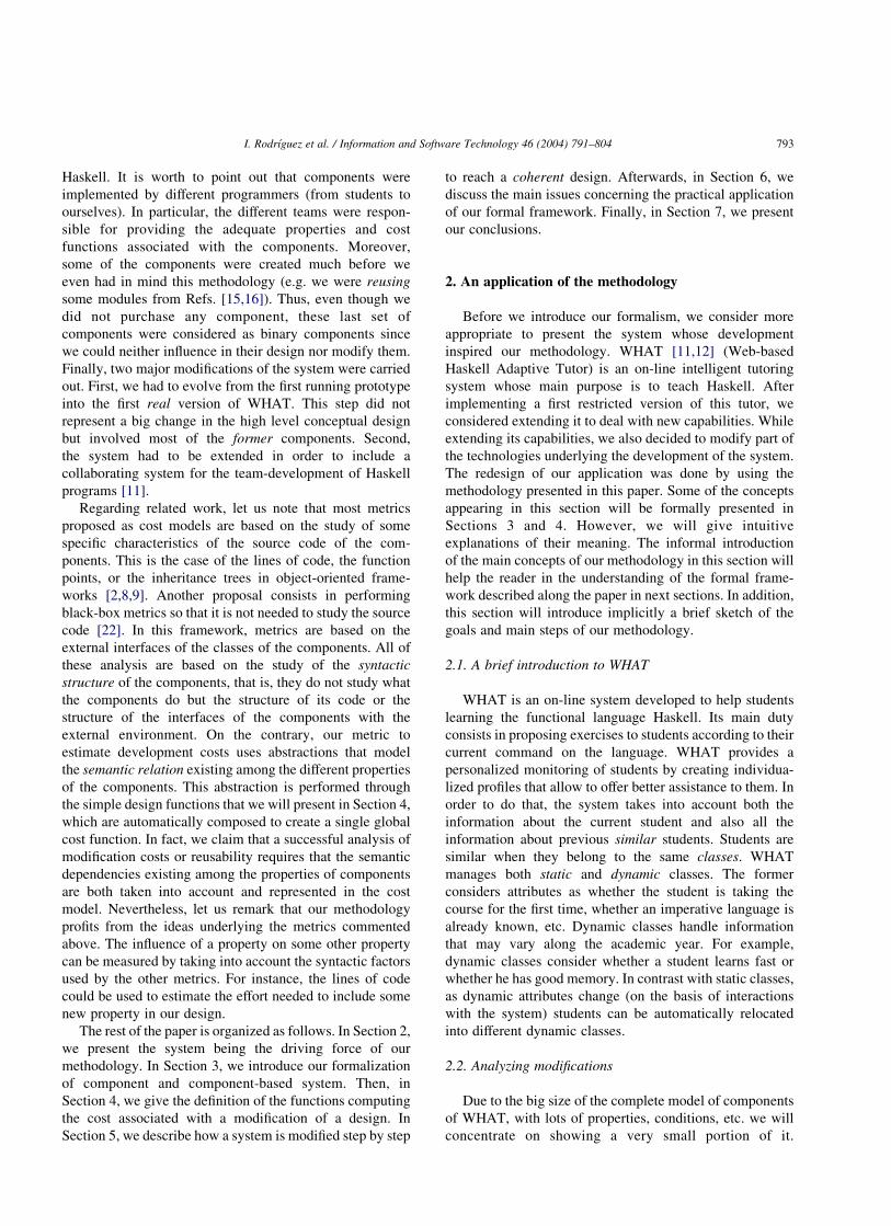
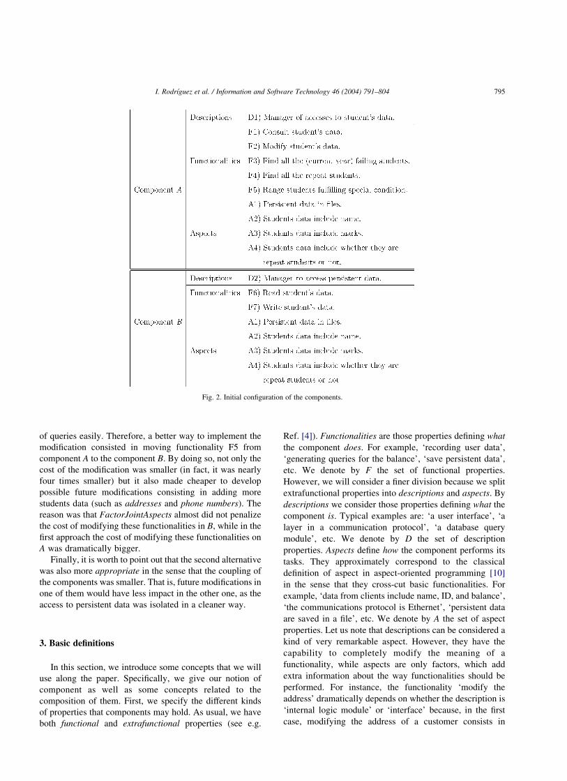
Specifically, we will present only two components. The first

one describes the logic of the management of student’s data

and the second one describes how the access to persistent

data is provided. The properties shown in this example are

just a small subset of the whole set of properties, so that we

may focus on this concrete example. As we will explain in

Section 3, a component has three kinds of properties

associated with it: descriptions (describing what the

component is), functionalities (describing what the com-

ponent does), and aspects (describing how the component

performs its tasks).

Let us consider the two components A and B depicted in

Figs. 1 and 2. The component A provides functionalities to

search information about students, but it has to use B in

order to access persistent data. In our first rudimentary

prototype, we handled the information about students by

using independent files for each student. However, when

developing the current version of WHAT, we decided to use

an Oracle database. As it can be expected, the decision of

using a different method to access persistent data forced a

modification in the design of the components.

In the rest of this section, we present how we dealt with

the previous modification. We will informally introduce

some of the functions where relations between components

as well as modification costs are encoded (formal definitions

of these functions will be given in Section 4).

In the initial version, as data were stored in different files,

ranging repeat students was tricky, as it forced handling the

files directly, searching for students fulfilling the required

conditions. Therefore, the functionalities F3 and F4 of the

component A forced F5 to be fulfilled. In fact, one of the

requirements of A is that a functionality for ranging students

must be available, no matter whether this functionality is

implemented by A or delegated to B: This requirement is

included in the function Func2Func, which for each

functionality states the other related functionalities (both

from the component and from the related components) that

must be fulfilled. Of course, the costs of performing these

searches were strongly influenced by the aspect saying that

persistent data were stored in files. This fact is included in

the definition of the function FactorAspect. This function

returns, for each functionality, the cost associated with

adapting the functionality to the corresponding aspect.

Besides, as a lot of information about students was stored,

ranging files was much more complicated than needed. As a

result, while including students data in persistent files,

FactorJointAspects penalized the costs associated with

ranging students. This function returns, for a given

functionality, the overhead generated because a set of

aspects must be simultaneously fulfilled.

Given the previous configuration, we proposed to modify

it so that persistent data were stored in an Oracle database.

Such a modification would imply the replacement of the

aspect A1 by a new aspect A5, meaning that persistent data

are stored in a database. Obviously, looking for students

with special characteristics would be easier with the new

configuration, since SQL queries were available. In fact, we

found two main methods to implement the modification, and

we computed the cost functions for each of them, using

programmer-hours as a unit to measure the costs. We used

this cost unit instead of money since the modification was

going to be performed by our students and us. Actually,

there was not money available to buy external components.

The first alternative consisted in keeping the low-level

search mechanism in the component A while modifying B to

substitute file management by database queries. The

functionalities of B would change, and their costs would

be estimated by using FactorAspect and FactorJointAs-

pects. Nevertheless, this approach was easily shown to be

inefficient, as database languages allow to perform this kind

Fig. 1. Diagram of configuration of components.


of queries easily. Therefore, a better way to implement the

modification consisted in moving functionality F5 from

component A to the component B: By doing so, not only the

cost of the modification was smaller (in fact, it was nearly

four times smaller) but it also made cheaper to develop

possible future modifications consisting in adding more

students data (such as addresses and phone numbers). The

reason was that FactorJointAspects almost did not penalize

the cost of modifying these functionalities in B; while in the

first approach the cost of modifying these functionalities on

A was dramatically bigger.

Finally, it is worth to point out that the second alternative

was also more appropriate in the sense that the coupling of

the components was smaller. That is, future modifications in

one of them would have less impact in the other one, as the

access to persistent data was isolated in a cleaner way.

3. Basic definitions

In this section, we introduce some concepts that we will

use along the paper. Specifically, we give our notion of

component as well as some concepts related to the

composition of them. First, we specify the different kinds

of properties that components may hold. As usual, we have

both functional and extrafunctional properties (see e.g.

Ref. [4]). Functionalities are those properties defining what

the component does. For example, ‘recording user data’,

‘generating queries for the balance’, ‘save persistent data’,

etc. We denote by F the set of functional properties.

However, we will consider a finer division because we split

extrafunctional properties into descriptions and aspects. By

descriptions we consider those properties defining what the

component is. Typical examples are: ‘a user interface’, ‘a

layer in a communication protocol’, ‘a database query

module’, etc. We denote by D the set of description

properties. Aspects define how the component performs its

tasks. They approximately correspond to the classical

definition of aspect in aspect-oriented programming [10]

in the sense that they cross-cut basic functionalities. For

example, ‘data from clients include name, ID, and balance’,

‘the communications protocol is Ethernet’, ‘persistent data

are saved in a file’, etc. We denote by A the set of aspect

properties. Let us note that descriptions can be considered a

kind of very remarkable aspect. However, they have the

capability to completely modify the meaning of a

functionality, while aspects are only factors, which add

extra information about the way functionalities should be

performed. For instance, the functionality ‘modify the

address’ dramatically depends on whether the description is

‘internal logic module’ or ‘interface’ because, in the first

case, modifying the address of a customer consists in

Fig. 2. Initial configuration of the components.


changing some data in the data base, while in the second

case it perhaps requires to modify the output in the screen.

In addition, descriptions play also the role of simple titles.

Definition 1. A component C is a tuple ðP;Po; tÞ; where P;

Po # D < F < A are the set of own properties and of

properties required to neighbors, respectively, and t is the

group of design functions for this component. We denote by

j the set of all components. A cost-evaluated component E

is a tuple ðP;Po;ModifCostÞ; where P and Po are as before

and

ModifCost : PðPÞ £PðPoÞ £PðPÞ £PðPoÞ! Rþ < {1}

is the function of modification cost. We denote by @ the set

of all cost-evaluated components.

As we indicated in Section 1, the description of a

component ðP;Po; tÞ is given by the properties fulfilled by

the component (i.e P), the properties expected from the

components this component depends on (i.e. Po), and a

group of design functions (i.e. t). In Section 4, we formally

present the kind of functions appearing in these tuples. They

give some basic values over the different kinds of properties.

A cost-evaluated component represents a different view of a

component. Intuitively, the group of design functions is

replaced by a cost function computing the cost associated

with the modification of the component by taking into

account the initial properties (first two arguments of

ModifCost) and the properties to be fulfilled after the

modification is performed (third and fourth arguments of

ModifCost). In Definition 2, we introduce two notions

related to systems of components.

Definition 2. A simple system of components S is a pair

ðK;GÞ; where we have that K # @ £N is a set of indexed

cost-evaluated components, and G : N!PðNÞ is the

directed dependencies graph of the system. A global system

of components GS is a tuple ðS;Av;MÞ; where S is a simple

system, Av is a set of pairs ðE;ModÞ denoting the available

cost-evaluated components E [ @ while Mod [{true; false} is a boolean denoting whether E can be

modified, and M : @! Rþ < {1} is a market denoting

the price of purchasing binary components, measured in

units of effort.

In the definition of simple systems, we consider that each

component has a unique identification number. Moreover,

for any i [ N we have that j [ GðiÞ; with ðE0; iÞ; ðE; jÞ [ K;

means that E0 depends on E: A simple system contains the

main information that we require, as presented in Section 1,

about a component based system (e.g. dependencies graph).

Global systems extend the notion of simple system to

consider that components can be bought. Let us remark that

bought components cannot be modified because we will not

(usually) receive the source code. Besides, global systems

also include information regarding the components, which

are freely available to the designer. These components

originate in either current and previous versions of used

components or in previous purchases.

4. Generation of the cost functions

In this section, we present the definition of the functions

computing the cost of performing a modification in a

component-based system. First, we give a set of simple

functions, each of them dealing with different kinds of

properties. Afterwards, we show how these simple functions

are combined to compute the overall cost function.

4.1. Generating design functions

Given a component and its current properties, the

function of modification cost computes the costs required

to modify its current properties so that it fulfills some new

desired properties. Obviously, the number of different

combinations of current and desired properties that could

be taken into account is huge. Thus, it is not feasible for a

designer to define all these cases. In contrast, a method

allowing the designer to specify a default pattern should be

provided, but the definition of as many special cases as

needed must be allowed. Following these ideas, in our

framework, the designer will only need to declare some

rules for each property (based on heuristics). For example,

we consider that a change into a configuration where the

properties of the component to be modified and those of the

related components are similar will be less expensive than a

change into a configuration where these properties diverge.

In addition, the relations among the different properties

must be defined. After that, an automatic process will

compute the appropriate costs description function.

The key point to make feasible the previous approach

consists in finding an adequate set of basic rules. On the one

hand, this set should be simple enough to allow the

developer to easily use the rules. On the other hand, it

should be expressive enough to provide the user with a

useful tool. The rest of this section presents a set of basic

definitions that will represent such a compromise between

expressivity and feasibility. We will classify them into two

main categories: those related to the modification of the

properties of the component itself and those related to the

modification of the properties that the component requires

from other components.

Our set of design functions will split the main semantic

features of components following the fundamental ideas of

aspect-oriented programming [10]. AOP proposes to split

the characteristics of programs into functionalities (what to

do) and aspects (how to do it) because the cross-cutting of

them is one of the main causes of coupling in real designs. In

our approach, this conceptualization will not be used to


provide a decoupled programming model, but to build a

rational semantic decomposition of the characteristics we

have to reason about. For example, our functions will set the

costs of including a functionality prior to consider any other

factor (e.g. 30 min to perform each operation of a matrix

operators module), the way the inclusion of an aspect would

influence the cost of implementing a functionality (e.g. time

multiplier of 5 if we want these operations to be specially

efficient, due to the special learning we need), the possibility

to use the code of other functionality whose implementation

is similar (e.g. including a functionality to perform the

multiplication of matrixes by vectors induces no new cost if

our code already have a functionality to multiply matrixes

between them), etc.

Let us start by describing the information required to

express the modification of the properties of the component.

We consider three kinds of properties depending on what

must be modified: descriptions D; functionalities F; and

aspects A:

When considering descriptions we need to take into

account three points. First of all, sometimes different

descriptions will share some common functionalities. In

these cases, we can reduce the costs associated with

modifying a description by taking advantage of the

similarities of the functionalities. Thus, we are interested

in the ratio of the costs that we will save due to similarities.

We define the function

Similarity : D £ D ! ½0; 1�

where Similarityðd1; d2Þ returns the proportion of the

functionality of d1 which can be applied to d2: The default

value is 0, while a value 1 means that d1 is a generalization

of the description d2: As a second cost, depending on the

complexity of a description, there will be a fix base cost to

develop any concrete functionality. We define this cost

DescripBaseCost : D ! Rþ

where DescripBaseCostðdÞ denotes the base cost associated

with the application of a functionality to the description d:

The default value is 0. As a final issue related to

descriptions, the cost to develop a description is multiplied

by a certain factor when it is being developed together with

other descriptions. Thus, we consider a function

Multiplicity : PðDÞ! Rþ

where 1 is the value by default.

In the case of functionalities, we also have to consider

several issues. First, and analogously to the previous case,

each functionality has a base cost. Thus, we have the

function

BaseCost : F ! Rþ

where BaseCostðf Þ denotes the cost needed to perform

functionality f without any other consideration, being 0 the

default value. Second, we can reduce the costs of

implementing a functionality by using similarities with

other functionalities already implemented. This fact is

considered by the function

ReusingSavings : F £ F ! ½0; 1�

where ReusingSavingsðf1; f2Þ defines the ratio of the

functionality f2 that can be saved by using functionality f1:

In this case, the default value is 0. Alternatively, the value 1

indicates again that f1 is a generalization of the functionality

f2: Third, a functionality can modify its cost by applying a

given aspect to it, multiplying its base cost by a certain

factor. This is reflected in the function

FactorAspect : F £ A ! Rþ

where the default value is 0. This value means that the

aspect a has no influence on the functionality f when

applying FactorAspectðf ; aÞ: Finally, the occurrence of

several aspects while developing a functionality can also

introduce a multiplicative factor in its cost. We consider the

function

FactorJointAspects : F £PðAÞ! Rþ

where 1 is the default value and represents that there is no

influence.

Let us consider now the influence of aspects. In this case,

we will have to consider three issues. First, the base cost

factor due to applying an aspect is given by

AspectBaseCost : A ! Rþ

being 0 the default value. Second, for each functionality, the

cost needed to migrate from an aspect to another is given by

the function

Migration : A £ A ! ½0; 1�

where Migrationða1; a2Þ defines the cost saved when

migrating from aspect a1 to aspect a2; or when adding a2

if a1 already exists. Also in this case we have that a value 1

means that a1 is a generalization of aspect a2; while 0 is the

default value. Finally, when including several aspects

simultaneously, a multiplicative factor must be considered,

representing the compatibility of such aspects:

Compatibility : PðAÞ! Rþ

being 1 the default value.

Next we present the functions related to the modification

of the properties required to neighbor components. In

addition to the own properties of the component (rep-

resented by D; F; and A) we will consider three more

categories denoting the properties the component requires

from related components. These categories are Do; Fo; and

Ao; representing descriptions, functionalities, and aspects,

respectively. In order to formalize the conditions that must

be fulfilled, we will use formulas of propositional logic in

which the proposition symbols of the signature represent

both own and required properties. We will denote by LðSÞ

the set of propositional formulas which can be built from

the signature S: Besides, we will assume that a valuation


n : S! {true; false} is available such that nðpÞ evaluates to

true iff the property p holds in the component. Let us note

that p can be either an own property of the component or a

property the component requires to its neighbors. We denote

by 4ðSÞ the set of all possible valuations over S: Besides,

we consider an evaluation function

Eval : LðSÞ £4ðSÞ! {true; false}

such that Evalðw; nÞ represents the evaluation of the

propositional formula w with valuation n:

Each basic function related to requirements of neighbor

properties provides a propositional formula which must hold

in a coherent design. With respect to descriptions, two

issues must be considered. The first one is related to the

implications that a description of a component has on other

descriptions. We have the function

Desc2Desc : D ! LðD < DoÞ

where Desc2DescðdÞ denotes the conditions (both internal

and external) that must be fulfilled when the description d

holds. The default value is the formula true; denoting that

nothing is required. The second issue is related to the

implications that a description of the component have on the

functionalities, both of the own component and of those of

the neighbors:

Desc2Func : D ! LðF < FoÞ

In the case of functionalities and aspects, the functions

needed are analogous. Implications of a functionality on

other functionalities, of the own component and of those of

the neighbors, are encoded in the function

Func2Func : F ! LðF < FoÞ

Besides, the implications of a functionality on the aspects

(both internal and external) are given by

Func2Asp : F ! LðA < AoÞ

Finally, the implications of an aspect on other aspects of

both the own component and of those of the neighbors

appear in the function

Desc2Func : A ! LðA < AoÞ

4.2. Generation of the global cost function

Once we have defined the basic functions to compute

costs we automatically obtain the global cost function. Let

us remark that the user will not need to define complex

functions like the ones that will be shown in this section: It

will be enough to define the simple functions presented in

Section 4.1 and the whole cost function will be automati-

cally obtained.

The generation of the modification cost function will

lie in the idea that the only thing that generates new

costs is to deal with functionalities. However, depending

on the factors that cross-cut these functionalities, these

costs will be modified. Thus, including a new aspect

generates new costs because it forces us to modify the

functionalities. Basically, costs will be split into those

derived from the modification of old functionalities and

those derived from the creation of new functionalities in

our components. Both of these costs will depend on the

descriptions and aspects required to hold. For instance,

the multiplying factors denoting the influence of aspects

on functionalities (given by the corresponding design

function) are taken into account by the modification cost

function by multiplying them by the base costs needed to

create the new functionalities (which are also given by

their own design function). Besides, in order to consider

the possibility of saving some costs, the modification cost

function tries to find the old functionality, which is most

similar to the new functionality we want to create. By

doing so, the modification cost function takes into

account that the new functionality could be created by

taking advantage of another functionality instead of

creating it from scratch. In addition, all the constraints

concerning the properties a component requires to other

components will be required to hold. Let us present

formally these ideas.

Let t denote a group of design functions, where each of

them is denoted by its sort (e.g. Similarity denotes the

Similarity function). The cost function generated from t;

denoted by GeneratedðtÞ; is a function

ModifCost : PðPÞ £PðPoÞ £PðPÞ £PðPoÞ! Rþ < {1}

where P ¼ D < F < A and Po ¼ Do < Fo < Ao: Intuitively,

ModifCostða1;g1;a2;g2Þ denotes the cost of modifying a

component having certain own and demanded properties

(a1 and g1; respectively), to reach the future own and

required properties (a2 and g2; respectively). In this case, a

value equal to 1 denotes that the modification is impossible.

The function ModifCost is defined as follows:

ModifCostða1;g1;a2;g2Þ

¼Old þ New if CondHolds ¼ true

1 if CondHolds ¼ false

(

In the previous expression, Old denotes the cost due to

the adaptation of old functionalities, New is the cost due to

the creation of new functionalities, and CondHolds indicates

that all of the condition functions hold. These values are

formally defined in Figs. 3–5, respectively.

Next we give an intuitive explanation of the meaning of

the definitions appearing in these figures. In the definition of

CondHolds in Fig. 3 the terms d2; f2; and a2 denote the set of

own properties after the modification, and do2; fo2; and ao2

denote the sets of properties demanded to neighbors after

the modification. Thus, CondHolds requires that the specific

conditions of any description, functionality, and aspect


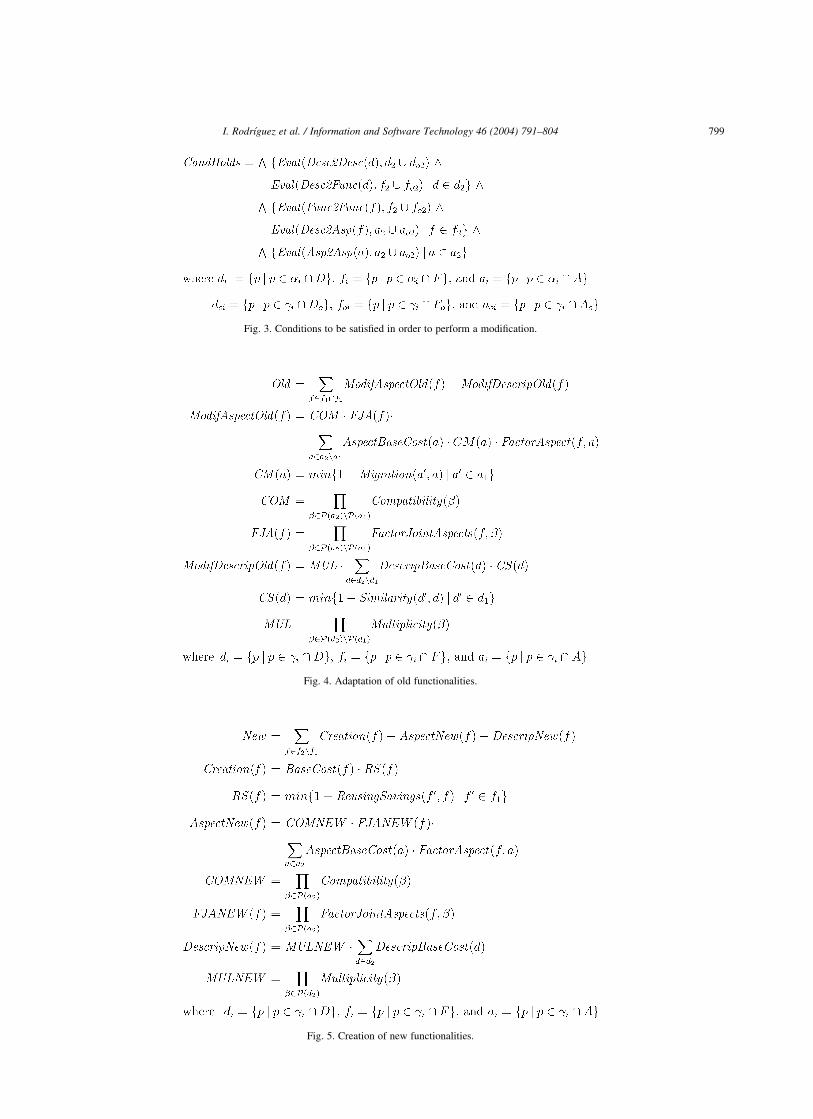
Fig. 3. Conditions to be satisfied in order to perform a modification.

Fig. 4. Adaptation of old functionalities.

Fig. 5. Creation of new functionalities.


existing in the new component hold after the modification is

performed.

In Fig. 4 we show the costs needed to adapt old

functionalities. These costs are split into those due to

modifications in the aspects and those incurred due to

modifications in the descriptions. When aspects change, the

main cost for adapting the functionality is computed by

adding all the AspectBaseCost’s, that is, by adding the base

costs of all of the new aspects. However, this cost must be

adjusted by taking into account both migration costs and

compatibility of the aspects. These factors have to be

adapted to the concrete functionality by using the functions

FactorJointAspects and FactorAspect. Analogously to the

case of modifying aspects, the costs due to changing the

descriptions are computed by adding the DescripBaseCost’s

reduced by the similarity factor, and increased by the

multiplicity factor.

Fig. 5 contains the costs related to the addition of new

functionalities. We can split these costs into three parts. The

cost due to aspects is the sum of the AspectBaseCost’s,

increased by the Compatibility factor, and adapted by using

the factors of the concrete functionality (FactorAspect and

FactorJointAspects). The cost due to descriptions is

computed from the sum of the DescripBaseCost’s, by

increasing them with the multiplicity factor. Finally,

reutilization costs are obtained by applying the ReusingSav-

ing to Base-Cost.

The generation of the cost function from the design

functions allows to use cost-evaluated components instead

of components. Actually, by applying Definition 1, a

component C ¼ ðP;Po; tÞ; where t is a group of design

functions, will be transformed into the cost-evaluated

component E ¼ ðP;Po;GeneratedðtÞÞ: From now on, only

cost-evaluated components will be used, as we will focus on

modification costs to develop our methodology.

5. Transformation of global systems

In Section 4.2, we showed how the global cost induced

by a modification can be computed. Next, we present a

mechanism to transform a global system where a modifi-

cation must be introduced. A valid transition represents a

single step in the process of eliminating incoherence by

replacing/modifying/purchasing a component.

Definition 3. Let GS ¼ ðS;Av;MÞ and GS0 ¼ ðS0;Av0;MÞ be

global systems such that S ¼ ðK;GÞ and S0 ¼ ðK 0;GÞ:

Intuitively, given two global systems GS and GS0; transition

GS ) c; bGS0 denotes that the cost of passing from GS to

GS0 is given by c: The second parameter of the transition,

that is b; is a boolean indicating whether a new component is

purchased or not.

Let c [ R and b [ Bool: We say that GS )c;b GS0 is

a valid transition if c – 1 and there exist two

cost-evaluated components E ¼ ðP;Po;CostModif Þ and

E0 ¼ ðP0;P0o;CostModif 0Þ such that ðE; iÞ [ K for some

i [ N; and K 0 ¼ ðK w {ðE; iÞ}Þ< {ðE0; iÞ}: In addition, the

conditions of one of the following cases hold:

† Modification of a component. In this case, c ¼

CostModif ðP;Po;P0;Po

0Þ; b ¼ false; ðE; trueÞ [ Av;

Av0 ¼ Av < {ðE0; trueÞ}; and CostModif ¼ CostModif 0:

† Substitution of a component by an existing component.

The conditions to be fulfilled are c ¼ 0; b ¼ false;

ðE0;XÞ [ Av with X [ {true; false}; and Av0 ¼ Av:

† Substitution of a component by the modification of an

existing component. There exits ðE00; trueÞ [ Av with

E00 ¼ ðP00;P00o;CostModif 0Þ; b ¼ false; c ¼

CostModif 0ðP00;P00o;P

0;P0oÞ; and Av0 ¼ Av < {ðE0; trueÞ}:

† Purchase of a binary component. c ¼ MðE0Þ; b ¼ true;

and Av0 ¼ Av < {ðE0; falseÞ}:

Let us remind that MðE0Þ denotes the cost (in units of

effort) of purchasing the component E0: Besides, let us note

that the third case generalizes the first two ones. However,

for the sake of clarity, we prefer to keep redundancy in

Definition 2. Among all the valid transitions leading to a

desired global system, we have to consider the cheapest

transition such that no component is purchased. Moreover,

we also take into account those transitions where a

component is purchased but its cost is cheaper than the

previous one. So, we will have a set of interesting transitions

to make any transformation of the system. The reason why

we require purchased components to be cheaper that

handmade components is that they are, in general, binary

and cannot be modified, which is a drawback against those

components that are directly developed by the team.

Definition 4. Let GS ¼ ðS;Av;MÞ be a global system such

that S ¼ ðK;GÞ: Let AðGS; S1Þ ¼ {GS )c;b GS0lGS0 ¼

ðS1;Av0;M0Þ} denote the set of transitions leading to the

same (final) simple system S1 and let cmin [ R be such that

cmin ¼ min{clðGS )c;b GS0Þ [ AðGS; S1Þ ^ b ¼ false}: We

define the set of interesting transitions for GS and S1;

denoted by InterestingðGS; S1Þ; as X1 < X2; where

X1 ¼ {ðGS )c;b GS0Þ [ AðGS; S1Þlb ¼ false ^ c ¼ cmin}

X2 ¼ {ðGS )c;b GS0Þ [ AðGS; S1Þlb ¼ true ^ c , cmin}

Next, we introduce the notion of coherent system, that is,

a system where all the requirements demanded by

components to neighbor components are fulfilled.

Definition 5. Let GS ¼ ðS;Av;MÞ be a global system

such that S ¼ ðK;GÞ: Let E ¼ ðP;Po;ModifCostÞ be


a cost-evaluated component such that ðE; iÞ [ K; for some

i [ N: We say that the conditions of the component E are

satisfied in GS; denoted by SatisfiedðE;GSÞ; if we have

Po # {P0lðE0; i0Þ[K ^ i0 [GðiÞ^E0 ¼ ðP0

;P0o;ModifCost0Þ}

We say that GS is coherent, denoted by CoherentðGSÞ; if for

any E such that ðE; iÞ[K; for some i[N; we have

SatisfiedðE;GSÞ:

In order to reach coherent systems we will use traces,

that is, sequences of concatenated interesting transitions.

Definition 6. A trace s is a finite sequence

½GS1 )c1;b1GS2;GS2 )c2;b2

GS3;…;GSn21 )cn21;bn21GSn�

of interesting transitions. The cost of the trace s; denoted by

costðsÞ; is defined asPn21

i¼1 ci: Besides, we say that s is a

coherent modification of GS1; denoted by

CoheModðGS1;sÞ; if CoherentðGSnÞ ¼ true:

Next, we define the objectives of the modifications.

These objectives are given by the set of new properties that

each component has to fulfill in the global system. We will

also characterize those systems fulfilling these new proper-

ties as well as the traces allowing to reach them. Moreover,

we can consider those traces reaching a global coherent

system GS such that the expected requirements are fulfilled.

Definition 7. Let GS ¼ ðS;Av;MÞ be a global system such

that S ¼ ðK;GÞ: A set of new requirements is a set of pairs

ði;PropÞ where i is the (unique) identification number of a

cost-evaluated component E associated with GS (that is,

ðE; iÞ [ K) and Prop is a set of new (own) properties

required to E: We say that GS fulfills the set of new

requirements R; denoted by fulfillðGS;RÞ; if for any

ði;PropÞ [ R we have that there exists E ¼

ðP;Po;CostModif Þ such that ðE; iÞ [ K and Prop # P:

A trace s ¼ ½GS1 )c1;b1GS2;…;GSn21 )cn21;bn21

GSn� is

an initial inclusion of the set of new requirements R and the

global system GS1; denoted by inclusionðR;GS1;sÞ; if

fulfillðGSn;RÞ ¼ true:

Let GS1 be a global system and R be a set of new

requirements. Let us consider a trace s ¼ ½GS1 )c1;b1

GS2;…;GSn21 )cn21;bn21GSn� such that

inclusionðR;GS1;sÞ and CoheModðGS1;sÞ: In this case,

we say that the trace s is an appropriate modification of GS1

according to R and we denote it by ApproModðGS1;R;sÞ:

Now that we have a method to reach a coherent design

fulfilling the new requirements, we can choose among the

possible solutions the most suitable one for our purposes.

However, we may also have in mind a list of modifica-

tions/additions to be included in future releases of our

system. We consider that possible future modifications are

described as a set Q such that each of its elements is a set of

new requirements. In this case, we may use the following

notion.

Definition 8. Let GS1 be a global system, R be a set of new

requirements, and Q be a set of possible future modifi-

cations. Let

s1 ¼ ½GS1 )c1;b1GS2;…;GSn21 )cn21;bn21

GSn�

s2 ¼ ½GSn )cn;bnGSnþ1;…;GSnþm21 )cnþm21;bnþm21

GSnþm�

be two traces such that ApproModðGS1;R;s1Þ and there

exits R0 [ Q such that ApproModðGSn;R0;s2Þ: In this case,

we say that the trace s ¼ s1+s2 is an appropriate

predictable modification of GS1 according to R and Q and

we denote it by ApproPredModðGS1;R;Q;sÞ:

In Definition 7, s1+s2 denotes the concatenation of the

traces s1 and s2: Let us note that costðsÞ ¼ costðs1Þ þ

costðs2Þ: We finish this section by showing an interesting

characterization of the degree of coupling among com-

ponents. Intuitively, if we have a new requirement for a

component E and an appropriate modification changes

another component E0 then we consider that E and E0 are

coupled.

Definition 9. Let GS1 ¼ ðS;Av;MÞ be a global system such

that S ¼ ðK;GÞ and let R ¼ {ðj;PropÞ} be a (unitary) set of

new requirements. Let E; E0 be cost-evaluated components

such that ðE; jÞ [ K and E0 ¼ ðP0;P0o;CostModif 0Þ; with

ðE0;mÞ [ K; for some m [ N: Let us consider a trace

s ¼ ½GS1 )c1;b1GS2;…;GSn21 )cn21;bn21

GSn�

such that GSn ¼ ðS0;Av0;M0Þ with S0 ¼ ðK 0;G0Þ: We say that

the trace s is a coupled modification of E and E0 with respect

to R in GS; denoted by coupledðGS;E;E0;R;sÞ; if

ApproModðGS1;R;sÞ and there exists a component E00 ¼

ðP00;P00o;CostModif 00Þ such that ðE00;mÞ [ K 0 and P00 – P0:

Once we have presented concepts as costs, appropriate

modifications, and appropriate predictable modifications, it

is possible to automatically apply them to real systems.

Thus, they can guide us while searching for the cheapest

modifications, the designs easier to modify, or the designs

with the smallest coupling factors. This can be done in such

a way that the designer does not need to perform by hand a

planning of all the changes that are needed to solve the

dependency issues. Actually, once the designer specifies the

system including the description of the components (own

properties, properties demanded to other components,

simple design functions), the dependencies among the

components (that is, the dependencies graph), and (option-

ally) a set of market components with their sale prices, then

any possible modification of the system can be analyzed in


an automatic way, returning data about modification costs,

degree of reusability, and degree of coupling. So, a designer

can use our methodology to study a set of possible design

alternatives, comparing the estimated results returned

automatically and choosing manually the solution which

better fits into her necessities according to her experience.

6. Methodological process

In this section, we discuss the main issues that must be

taken into account concerning the practical application of

our formal framework. We will provide a guideline of the

methodology, and we will identify the parts of our

framework that can be automatized.

According to the previous sections, we can split the

estimation process into three phases:

(1) Providing basic design functions to estimate the cost of

modifying basic simple semantic properties.

(2) Providing a function to estimate the cost of modifying

a component from a previous configuration to a new

configuration.

(3) Providing a mechanism to estimate the cost of

modifying a system to include a new set of

properties in such a way that the consistence

among component dependencies is kept.

Let us note that, in spite that the first phase cannot be

automatized and is (relatively) expensive for users in terms

of training and analysis, phases two and three can be

completely automatized once the previous analysis has been

done. Actually, both the generation of the modification cost

function from the design functions and the estimation of the

cost needed to modify the whole system are formally

defined in Sections 4.2 and 5, respectively. Only a formal

definition of them would allow a computer to study

automatically and without ambiguity all (or a huge amount

of) the possibilities to deal with a modification in a system.

Thus, formalization is a must for automatization of phases

(2) and (3). In order to develop an automatic analysis, it is

enough to develop a tool that applies each definition in

Sections 4.2 and 5 one after each other. If it is the case that

we want to perform a systematic search of possible ways to

perform a modification, it must be taken into account the

combinatorial explosion of possibilities that appears. This is

because each decision regarding whether some modification

should be kept in one component or propagated to other

components opens a new set of possibilities. However, the

problem of considering a huge amount of different

possibilities will be dealt more efficiently by a machine

than by a designer, specially since the estimated cost for

each possibility is computed by applying some well-defined

but tedious arithmetic calculus. Thus, the main feature of

our approach is that the dirty work can be performed by a

machine after the designer provides some basic heuristics.

In order to apply our methodology, the data a software

engineer must provide consists of the decomposition of the

system into components, the properties of each of these

components, and the design cost functions. It is worth to

point out that functional issues are not always a good

criterium to make the partition of the system into

components, because components must be entities of

deployment oriented to reusability. The identification of

properties will not require in general a further analysis,

because these properties should have been defined in the

analysis and design phases in the project development

process (identification of descriptions and functionalities is

straightforward; aspects will be represented in general in the

form of analysis/design constraints). Regarding how to

obtain the design functions, that process must be based

mainly on the experience. Basically, we have to consider the

complexity of the hypothetical resulting code for each

specific case. This seems not to be so different to any other

estimation technique. However, the key in our framework is

that we estimate not the cost of the whole modification, but

the cost of each single piece of modification (functional-

ities) and the cost of each factor that could influence them

(aspects, descriptions), in such a way that any modification

resulting from any combination of these pieces of

modification may be obtained directly by performing an

automatic arithmetic operation. Thus, by providing simple

modification costs we automatically provide the cost of any

modification constructed from them.

In contrast with other cost estimation methods based on

syntactic issues (e.g. number of function calls in the future

code) where users almost do not need any special training,

our cost estimation proposes to take into account some

semantic factors. This is why we focus on considering

features like functionalities and aspects. We think that

(isolated) syntactic approaches for cost estimation are not

only shallow to make good estimations, but also useless to

provide an automatic mechanism to estimate the cost

needed to modify an application. Unless we provide a

relation between the specific things we want to do and their

possible costs, any a priori estimation will be impossible.

However, our methodology can benefit from these syntactic

approaches. Actually, the construction of each specific basic

design function can be performed by using any suitable

criterium. Hence, other approaches may help the software

engineer to build these functions, though our framework

will guide afterwards the automatic process to compose

them and to analyze modifications in the whole system.

Summarizing, our complete methodology can be split

into the following steps:

† First, we perform a partition of the design into

components. Let us remark that, as we said before,

components are reusable entities of deployment. Hence,


functional issues are not necessarily a good criterium to

perform such a partition. Basically, each component will

be a set of highly coupled elements such that the coupling

of these elements with the rest of the system is low.

† Afterwards, we provide the input data of our method-

ology, that is, we identify the specific descriptions,

functionalities, and aspects of each component.

† Then, we build the design functions for each component.

In order to reduce the number of cases to cover in

functions, we can set up some special design functions to

be used in all components, mainly those concerning

aspects. These ‘generic’ design functions represent a

trade-off between accurate estimations and effort needed

to make such estimations. For instance, aspects like the

influence of the specific programming language or the

performance issues could be considered as generic and

their influence on functionalities could be equally

computed. Other factors that are completely different in

different components deserve their own specific con-

siderations. This is mainly the case of functionalities.

† We calculate the whole cost modification function.

† Then, we specify the system we want to develop, finding

the new properties we need the components to fulfill.

Actually, this step could force us to include some aspects

and functionalities that were not considered initially in

the design functions, so some of them could have to

rewritten.

† Finally, we study alternatives to perform this modifi-

cation. These alternatives dealt with whether some

modification should be propagated to other components

or not. Similarly, we can compute the coupling of some

components with respect to some predictable future

modifications.

7. Conclusions

In this paper, we have presented a methodology to assist

in the process of modifying the design of a component-

based system. In particular, it provides analysis of the

impact of each modification. The method takes as input the

specification of the components, including the dependencies

structure, the properties that each component holds, and the

properties that each component requires from other

components. In addition to that, some functions are

provided in order to specify relations among properties.

Those functions facilitate the estimation of costs. All these

simple functions are used to automatically generate a single

global cost function. Taken into account this function, the

cost of each possible modification can be automatically

computed, enabling the systematic study of the different

alternatives to perform the desired modifications. This

systematic study includes information about costs, reusa-

bility, and coupling of the different alternatives.

We are aware that the use of our methodology requires a

certain degree of familiarity with the process, starting from

the identification of properties, and going through the

definition of the functions expressing these properties. We

are aware that our framework has only been tested with only

a single case study, and much more case studies are needed,

specially to compare its practical benefits with other less

formal cost estimation models. Nevertheless, despite the

apparent complexity, the experiments that we have

performed so far are very encouraging.

Acknowledgements

We would like to thank the anonymous referees for their

valuable comments during the evaluation process of this

paper. Work supported in part by the projects TIC2003-

07848-C02-01 and PAC-03-001.

References

[1] A. Brown, K. Wallnau, The current state of CBSE, IEEE Software

1998 (1998) 37–46.

[2] S. Chidamber, C. Kemerer, A metrics suite for object oriented design,

IEEE Transactions of Software Engineering 20 (6) (1994) 476–493.

[3] I. Crnkovic, Component-based software engineering: new challenges

in software development, Software Focus 2 (4) (2001) 127–133.

[4] I. Crnkovic, B. Hnich, T. Jonsson, Z. Kiziltan, Specification,

implementation, and deployment of components, Communications

of the ACM 45 (10) (2002) 35–40.

[5] I. Crnkovic, M. Larsson, Challenges of component-based develop-

ment, Journal of Systems and Software 61 (2002) 201–212.

[6] E. Gamma, R. Helm, R. Johnson, J. Vlissides, Design Patterns:

Elements of Reusable Object-oriented Software, Addison-Wesley,

Reading, MA, 1995.

[7] S.A. Hissam, G.A. Moreno, J. Stafford, K.C. Wallnau, Packaging

Predictable Assembly, in: IFIP/ACM Working Conference on

Component Deployment, LNCS 2370, Springer, Berlin, 2002, pp.

108–124.

[8] T. Capers Jones, Programming Productivity, McGraw-Hill, New

York, 1986.

[9] T. Capers Jones, Applied Software Measurement: Assuring Pro-

ductivity and Quality, McGraw-Hill, New York, 1991.

[10] G. Kiczales, J. Lamping, A. Menhdhekar, C. Maeda, C. Lopes, J.-M.

Loingtier, J. Irwin, Aspect-oriented Programming, in: 11th European

Conference on Object-oriented Programming, LNCS 1241, Springer,

Berlin, 1997, pp. 220–242.

[11] N. Lopez, M. Nunez, I. Rodrıguez, F. Rubio, Including Malicious

Agents into a Collaborative Learning Environment, in: Eighth

Intelligent Tutoring Systems, LNCS 2363, Springer, Berlin, 2002,

pp. 51–60.

[12] N. Lopez, M. Nunez, I. Rodrıguez, F. Rubio, WHAT: Web-based

Haskell Adaptive Tutor, in: 10th Artificial Intelligence: Method-

ologies, Systems, and Applications, LNAI 2443, Springer, Berlin,

2002, pp. 71–80.

[13] D. Mason, Probabilistic Analysis for Component Reliability Compo-

sition, in: Fifth ICSE Workshop on Component-based Software

Engineering, 2002.

[14] G.A. Moreno, S.A. Hissam, K.C. Wallnau, Statistical Models for

Empirical Component Properties and Assembly-level Property

Predictions: Toward Standard Labelling, in: Fifth ICSE Workshop

on Component-based Software Engineering, 2002.

[15] M. Nunez, P. Palao, R. Pena, A Second Year Course on Data

Structures Based on Functional Programming, in: Functional


Programming Languages in Education, LNCS 1022, Springer, Berlin,

1995, pp. 65–84.

[16] R. Pena, Y. Ortega-Mallen, F. Rubio, Teaching Monadic Algor-

ithms to First-Year Students, in: Workshop on Algorithmic

Aspects of Advanced Programming Languages, WAAAPL’99,

1999, pp. 33–45.

[17] I. Rodrıguez, F. Rubio, A Framework for Selecting Components

Automatically: A First Approach, in: TACOS’03—Test and Analysis

of Component Based Systems. Electronic Notes in Theoretical

Computer Science, 2003, p. 82.

[18] J. Rumbaugh, I. Jacobsen, G. Booch, Unified Modeling Language

Reference Manual, Addison-Wesley, Reading, MA, 1997.

[19] J. Stafford, J.D. McGregor, Issues in Predicting the Reliability of

Composed Components, in: Fifth ICSE Workshop on Component-

based Software Engineering, 2002.

[20] C. Szyperski, Component Software: Beyond Object-oriented Pro-

gramming, Addison-Wesley, Reading, MA, 1998.

[21] C. Szyperski, Components and the way ahead, in: G.T. Leavens, M.

Sitaraman (Eds.), Foundations of Component-based Systems, Cam-

bridge University Press, Cambridge, 2000, Chapter 1.

[22] H. Washizaki, H. Yamamoto, Y. Fukazawa, A Metrics Suite for

Measuring Reusability for Software Components, in: Proceedings of

the Ninth International Symposium on Software Metrics (Metrics

2003). IEEE CS, 2003.


Documents

A formal framework for analyzing reusability complexity in component-based systems