A frequency and knowledge tree/causality diagram based expert system approach for fault diagnosis

Refiability Engineering and System Safety 43 (1994) 17-28

A frequency and knowledge tree/causality diagram based expert system approach for

fault diagnosis

Qin Zhang* Institute of Nuclear Energy Technology, Tsinghua University, Beijing 100084, People's Republic of China

(Received 16 November 1992; accepted 26 April 1993)

Developed from the initial idea presented in a companion paper (Zhang, Q. et al., Reliability Engng System Safety, 34 (1991) 121-42), a novel frequency and knowledge tree/causality diagram based expert system approach for the on-line/off-line fault diagnoses of engineering systems such as nuclear power plants is presented in this paper. The newly made progress includes the modular knowledge base construction, how to utilize the information of the order of signal appearance, how to express uncertainties of experts' opinions in the tree based knowledge bases, how to find the possible fault hypotheses and propagate uncertainties through the time-specific knowledge trees or causality diagrams that may include many loops, and how to deal with the imperfectness of knowledge bases and unknown signals. A tutorial example is included to illustrate the methodology.

I INTRODUCTION

There has been an increasing interest in the development of expert systems for fault diagnosis of engineering systems such as nuclear power plants, chemical facilities, etc. With the help of such expert systems, operators of plants may find the failures or root causes of abnormalities in plants more efficiently and accurately, in particular in emergency cases, so that an accident may be controlled in time. With such a help, the human errors during fault diagnosis and decision-making may be reduced significantly, there have been many expert system approaches. 2-9 Some of them do not consider uncertainties (e.g. Refs 2-4) and the others consider (e.g. Refs 5-9) in which some of them are based on the Bayesian theory 5'6 and the others are not. 7-9 The overview of all of these approaches is itself an interesting topic of an independent paper and is not intended to be addressed here. However, it is noted that there is a

*Present address: Technological Innovation Corp. of Xiamen, 18/F Huguang Building, Hubin Dong Lu, Xiamen 361 004, People's Republic of China.

Reliability Engineering and System Safety 0951-8320/94/$06.00 © 1994 Elsevier Science Publishers Ltd, England.

17

common issue for all of these approaches: how to construct a knowledge base in such a way that the domain experts/engineers can easily understand and follow and then they can construct the knowledge base by themselves even without the help of knowledge engineers. One solution to this problem may be the modular knowledge construction as, for example, shown in Pearl's belief network 6 in which one needs only to consider the direct dependencies of a node with other nodes regardless of the indirect dependencies. However, such a treatment may result in cause-consequence loops in knowledge base. Thus, how to break down these loops in inferences without increasing the computation amount too much is then the subsequential issue. Moreover, when considering uncertainties, the Bayesian approach needs to consider how to avoid dealing with the restriction Pr{B ] E} + Pr{B I E} = 1 that may not be realistic when probabilities are used to quantify the degree of experts' belief on something or, in other words, when the probabilities are subjective, 7 where B is an event and E is the evidence.

Developed from the initial idea presented in our companion paper, 9 a novel frequency and time- specific modular knowledge tree or, more intuitively, causality diagram based expert system approach for fault diagnoses is presented in this paper, in which the

18 Qin Zhang

knowledge base consists of the modular knowledge trees that are very similar to the well-known fault trees and can be easily understood and followed by most domain experts/engineers. The inference mech- anism in this approach is capable of breaking down the cause-consequence loops without increasing the computation amount significantly. Uncertainties are considered based on the Bayesian theory without dealing with the restrict mentioned above. In Ref. 9, we have introduced the frequency-based approach and the tree-based knowledge representation. In this paper, the modularity of the tree-based knowledge base is further addressed. Moreover, the newly made progress in this paper also includes (i) how to utilize the information of the order of signal appearance that is useful for more accurate diagnosis; (ii) how to express uncertainties of experts' opinions in the tree-based modular knowledge bases in which tree 1 may be an input of tree 2 while tree 2 is an input of tree 1; (iii) how to find the on-line possible fault hypotheses and propagate uncertainties through the time-specific knowledge trees or causality diagrams that may include many loops; and (iv) how to deal with the imperfectness of knowledge bases and unknown signals.

It is noted that in some approaches (e.g. Ref. 2), signals are first verified through signal validation by incorporating deep plant knowledge. In this approach, if such a signal validation module is available, it can be used as a signal filter before the signals are used as the evidence in the inference, and may then result in more accurate diagnostics. However, the signal validation is not a necessary module in this approach because the spurious sensor signals can be found through the inference process (see section 2.4).

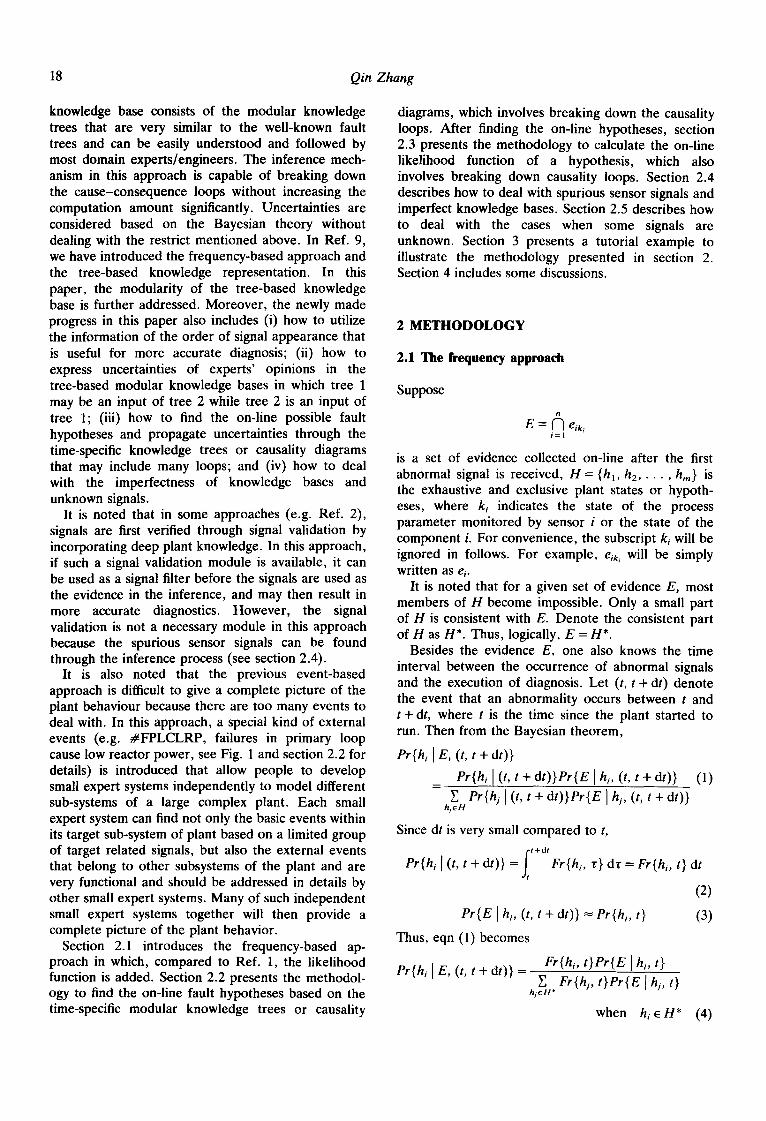
It is also noted that the previous event-based approach is difficult to give a complete picture of the plant behaviour because there are too many events to deal with. In this approach, a special kind of external events (e.g. #FPLCLRP, failures in primary loop cause low reactor power, see Fig. 1 and section 2.2 for details) is introduced that allow people to develop small expert systems independently to model different sub-systems of a large complex plant. Each small expert system can find not only the basic events within its target sub-system of plant based on a limited group of target related signals, but also the external events that belong to other subsystems of the plant and are very functional and should be addressed in details by other small expert systems. Many of such independent small expert systems together will then provide a complete picture of the plant behavior.

Section 2.1 introduces the frequency-based approach in which, compared to Ref. 1, the likelihood function is added. Section 2.2 presents the methodology to find the on-line fault hypotheses based on the time-specific modular knowledge trees or causality

diagrams, which involves breaking down the causality loops. After finding the on-line hypotheses, section 2.3 presents the methodology to calculate the on-line likelihood function of a hypothesis, which also involves breaking down causality loops. Section 2.4 describes how to deal with spurious sensor signals and imperfect knowledge bases. Section 2.5 describes how to deal with the cases when some signals are unknown. Section 3 presents a tutorial example to illustrate the methodology presented in section 2. Section 4 includes some discussions.

2 METHODOLOGY

2.1 The frequency approach

Suppose

E = f~ elk i i=l

is a set of evidence collected on-line after the first abnormal signal is received, H = {hi, h2 . . . . . h,,} is the exhaustive and exclusive plant states or hypotheses, where k~ indicates the state of the process parameter monitored by sensor i or the state of the component i. For convenience, the subscript k; will be ignored in follows. For example, eik, will be simply written as e~.

It is noted that for a given set of evidence E, most members of H become impossible. Only a small part of H is consistent with E. Denote the consistent part of H as H*. Thus, logically, E = H*.

Besides the evidence E, one also knows the time interval between the occurrence of abnormal signals and the execution of diagnosis. Let (t, t + dt) denote the event that an abnormality occurs between t and t + dt, where t is the time since the plant started to run. Then from the Bayesian theorem,

Pr{hi I E, (t, t + dt)}

er{hi I (t, t + dt)}Pr{E I hi, (t, t + dt)} (1)

Pr{hj ](t, t + dt)}Pr(E ] hj, (t, t +dt)} hjeH

Since dt is very small compared to t, ~t+dt

Pr{hi [ (t, t + dt)} = Fr{hi, z} dz = Fr{hi, t} dt ~t

(2) Pr(E I hi, (t, t + dt)} = Pr{hi, t} (3)

Thus, eqn (1) becomes

Pr{hl I E, (t, t + d/)} = Fr{hi, t }Pr{E I hi, t} Fr{hj, t}Pr{E [hi, t}

hjeH*

when hi E H* (4)

Knowledge tree/causality diagram for fault diagnosis 19

t ~

I " ©

t ~ - -

LL

CL

_o

E

. m

t ~

E

i

20 Qin Zhang

otherwise

Pr{hi I E, (t, t + d/)} = 0

because er(E I hi, t} = O.

Where Fr{. } is a frequency function, Fr{hi, t} is the unconditional frequency of hi at time t, Pr(Elhi, t} reflects the confidence or belief of experts on the event that E will appear when hi occurs at time t.

For convenience, in what follows, the time variable t will be ignored and thus eqn (4) can be simply written as

Fr(h,}Pr{E [h,} when h i e H* Prln , l =

Fr{hi}Pr{Elhi} hi~H*

(5)

Equation (5) is similar to that in Ref. 5. In Ref. 5,

Pr{hi} fi Pr{ei ]hi} I = 1

Pr{hi I E} = (5')

E Pr{h i} [I Pr(e, [hi} hieH 1=1

assumed that el, l= 1 . . . . . n, are independent of each other conditioned by hi.

The differences between eqns (5) and (5') are: (i) eqn (5) uses Fr{hi} instead of Pr{hi} as in eqn (5') so that the frequency feature is directly indicated; (ii) I17-1 Pr{el I hi} in eqn (5') is replaced by er{E[hi} because el, 1 = 1 . . . . . n, are usually not independent of each other in our approach even conditioned by hi; (iii) H* and er(EIh i} in our approach are found on-line after E is received.

2.2 H o w to find H *

to find H*, we have

ei = SF~ + RiXi + Rdgi = Si + RiXi (6)

Si = SF~ + RiIKi (7)

2 -

H* = e = (s, + RiXi) = A S, A RiXi (8) i = l o¢=1 i~la J~J~

where '+ ' is the exclusive OR Operator; I~ +J~ = { 1 , . . . , n}; Ri denotes that sensor i is reliable; Xi denotes that what ei indicates is true; SF~ denotes that sensor i is malfunctioning or failed to function; IKi indicates the imperfectness of the mini knowledge tree (e.g. as shown in Fig. 1) that is intended but actually failed to explain Xi due to its imperfectness or incorrect interpretation of e/ as Xi, Si indicates that signal i should be ignored because of either the sensor failure or the imperfectness of the associated mini knowledge base.

It is noted that eqn (8) has the suspicion of the combination explosion of terms. However, in most

cases, all signals and corresponding knowledge bases are correct and only one term, i.e.

R;xi, i = l

is needed. In rare cases, one of the signals is spurious or its corresponding mini knowledge base is imperfect. In these cases, n or a little more additional terms are added, where the correlated mini knowledge bases due to common imperfectness are treated as a single mini-knowledge-base to be ignored. In very rare cases, more than one independent signals are spurious or have imperfect mini-knowledge-bases. In these cases, much longer computation time will be taken because of the increase of number of terms. Thus, in most cases, the combination explosion will not appear.

For the further development of H*, we treat each Xi in eqn (8) as a top event of a mini-knowledge-tree that serves as a mini-knowledge-base. These trees are developed in advance and their minimal cut sets are found and stored in computer as the knowledge bases. A minimal cut set is a combination of events that causes sufficiently the top event of the tree. The development of these mini trees is quite independent. When one develops a mini-tree, he/she needs only to know the local basic events and the top events of other trees. The top events of other trees are used as the input of the current tree. These local basic events and top events have direct dependencies with the current top event. That is, our knowledge bases are modularised. Users may combine them in different ways to construct different packages of knowledge bases to fit different plant operation modes. By using these mini-knowledge-bases, eqn (8) can be further expanded in terms of cut sets. These cut sets are then the detailed H*.

As an example, a mini-tree, SPLAL (steam pressure in line A is abnormally low), is shown in Fig. 1, which is used as a mini-knowledge-base of the main stream and feedwater condensate system of a nuclear power plant. In the tree, a circle means a basic event. If its name is marked with ' # ' , then it is an initiating event. If it is marked with ' - ' , then it is a complementary event. Otherwise, it is a non-initiating event. A diamond, its name is marked with '!', means a top event of another mini-tree that serves as an input of the current tree. The minimal cut sets of SPLAL are shown in Table 1, which are equivalent to the tree.

In our approach, the development of the mini trees follows the following rules:

(1) the top event must be associated with one of Xi in eqn (8);

(2) directly use the top events of other mini-trees as input (diamonds) whenever they are the causes; and

Knowledge tree~causality diagram for fault diagnosis 21

Table 1. The tat sets and c o d d e n c e factors of SPLAL

No. Cut sets CF

1 !TE1170L 0.8 2 #PCV308AO 1.0 3 #RAFO 1.0 4 #PT446FL 0.7 5 #FPLCLRP 0.8 6 !PT446L, -MSIVAC 1.0 7 #MSIVAC, PCV308AFR 1.0 8 #MSIVAC, RAFR 1-0

(3) include the OK events (complement of fault events, e.g. -MSIVAC in Fig. 1) in the tree whenever they are necessary to ensure that the employed causality linkage is not broken.

Obviously, the development of such mini-knowledge- trees are very simple so that the domain experts/engineers can do it by themselves without the help of knowledge engineers.

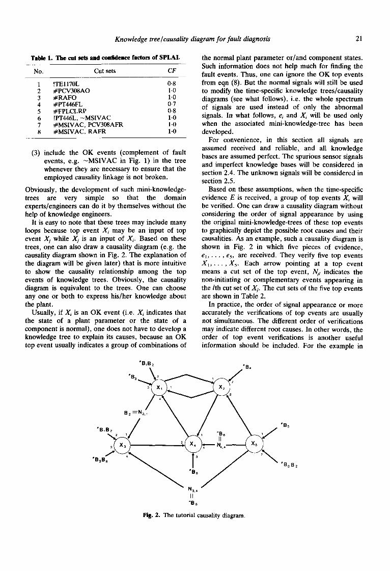
It is easy to note that these trees may include many loops because top event X~ may be an input of top event Xj while Xj is an input of Xi. Based on these trees, one can also draw a causality diagram (e.g. the causality diagram shown in Fig. 2. The explanation of the diagram will be given later) that is more intuitive to show the causality relationship among the top events of knowledge trees. Obviously, the causality diagram is equivalent to the trees. One can choose any one or both to express his/her knowledge about the plant.

Usually, if X; is an OK event (i.e. Xi indicates that the state of a plant parameter or the state of a component is normal), one does not have to develop a knowledge tree to explain its causes, because an OK top event usually indicates a group of combinations of

the normal plant parameter or/and component states. Such information does not help much for finding the fault events. Thus, one can ignore the OK top events from eqn (8). But the normal signals will still be used to modify the time-specific knowledge trees/causality diagrams (see what follows), i.e. the whole spectrum of signals are used instead of only the abnormal signals. In what follows, el and Xi will be used only when the associated mini-knowledge-tree has been developed.

For convenience, in this section all signals are assumed received and reliable, and all knowledge bases are assumed perfect. The spurious sensor signals and imperfect knowledge bases will be considered in section 2.4. The unknown signals will be considered in section 2.5.

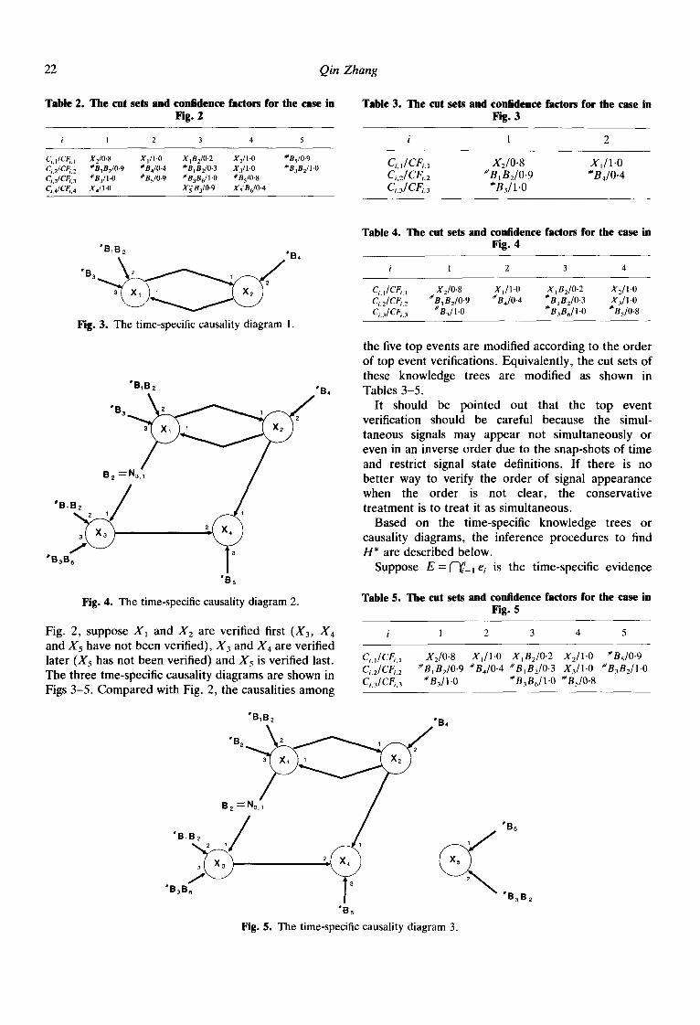
Based on these assumptions, when the time-specific evidence E is received, a group of top events X~ will be verified. One can draw a causality diagram without considering the order of signal appearance by using the original mini-knowledge-trees of these top events to graphically depict the possible root causes and their causalities. As an example, such a causality diagram is shown in Fig. 2 in which five pieces of evidence, el . . . . . es, are received. They verify five top events X~ . . . . . Xs. Each arrow pointing at a top event means a cut set of the top event, Nil indicates the non-initiating or complementary events appearing in the lth cut set of ,ks. The cut sets of the five top events are shown in Table 2.

In practice, the order of signal appearance or more accurately the verifications of top events are usually not simultaneous. The different order of verifications may indicate different root causes. In other words, the order of top event verifications is another useful information should be included. For the example in

"B~B2 ~'B4

B 2 ----" Na. 1

"B~B2 2 ~ # f ~ "Be ~ / Z,) 3l~ ^ = ) "PC "~, )41 N,,, L ~ ,)

It "B a

"B5

"BaB 2

Fig. 2. The tutorial causality diagram.

22 Qin Zhang

TaMe 2. The cut sets and confidence factors for the case in Fig. 2

i 1 2 3 4 5

Ci, IICFi, t X2/0.8 Xt/1-0 XIB2/0.2 X2/I.O #B5/0.9 Ci.21CFi, 2 ~aBIB2/0.9 #B4/0.4 #BIB2~0.3 X3/I.0 #B3B2/I.O ChflCFi. 3 #B3/I.0 #B5/0-9 #B3Br/1.O #B5/0.8 Ci,4/CFi. 4 X4/l-0 X~B3/0.9 X~B6/0.4

Table 3. The cut sets and confidence factors for the case in Fig. 3

i 1 2

Ci . l /CFi . I X 2 / 0 " 8 X , / 1 . O C,,2/ CF~,2 # B t B2/0.9 #B4/0.4 Ci,3/ CFi, 3 # B3/1.O


i 1 2 3 4

Ci.t/CFi. i X2/0"8 XI/I 'O XtB2/0"2 X2/1.0 Ci.2/CFi. 2 ~BIB2/0"9 #B4/0.4 ~ BIBz/0.3 X3/I.0 Ci.3/CFi. 3 '~B3/1.0 # B3B6/ I.O # B5/0.8

"B~B2 "B,

Fig. 3. The time-specific causality diagram 1.

"B~B2 "B,

B Na

*B~B 2

"B3B 13

Fig. 4. The time-specific causality diagram 2.

Fig. 2, suppose X~ and X2 are verified first (X3, X4 and X5 have not been verified), X3 and X4 are verified later (X5 has not been verified) and X5 is verified last. The three tme-specific causality diagrams are shown in Figs 3-5. Compared with Fig. 2, the causalities among

the five top events are modified according to the order of top event verifications. Equivalently, the cut sets of these knowledge trees are modified as shown in Tables 3-5.

It should be pointed out that the top event verification should be careful because the simultaneous signals may appear not simultaneously or even in an inverse order due to the snap-shots of time and restrict signal state definitions. If there is no better way to verify the order of signal appearance when the order is not clear, the conservative treatment is to treat it as simultaneous.

Based on the time-specific knowledge trees or causality diagrams, the inference procedures to find H* are described below.

E " Suppose = (-'li=~ ei is the time-specific evidence


i 1 2 3 4 5

Ccl/CFi. I XJO.8 XI/I.O XjBJO.2 X2/I.O #Bs/0.9 Ci.2/CFi, 2 #BIB2~0.9 #BJO.4 #BIB-,~0.3 S3/l .0 #B3B2/I.O Ci,3]Cfi. 3 #B3/1-0 #B3BJI'O #BJO'8

"B~B2 "B4 " B a ~

"B5 'B~Bz / /

"BaBe ,BaB2 ~Bs Fig. 5. The time-specific causality diagram 3.


on-line received and continuously updated. Since all signals and knowledge bases are assumed reliable, according to eqn (8),

According to the on-line

where R = f ~ R ; i = 1

(9)

updated time-specific mini-knowledge-trees, or equivalently but more intuitively the time-specific causality diagram,

x,: u c,,:(uNi, n ,Iu(uc,,t I~_L£r+Li,, I • J~Jilx I \l~Li, I

(10)

where (?it is the lth cut set of X~, Li~ is the index set of the cut sets that contain other top events, L~c is the index set of the cut sets of X,- without any other top events, N, is the non-initiating or complementary events associated with the lth cut set of the top event X~, J.x is the index set of the top events that are contained in the lth cut set of X~.

Let A~ be the index set of top events in a causality chain starting with X~ and ending at the last input top event (the case of open chain) or Xj again (the case of closed chain). For the example in Fig. 2, X4 ~ X5 is an open chain (A4 = {4, 5}) where Xs is the last input top event; X 3 ~ X j ~ X 2 ~ X 5 ~ X 4 ~ X 3 is a closed chain (A 3 = {3, 1, 2, 5, 4, 3}); X 3 ~ X s ~ X 4 ~ X 3 is another closed chain also starting with X3(A3 = {3, 5, 4, 3}), etc.

To expand eqn (9) by substituting eqn (10) into eqn (9), eqn (10) should be expanded first by repeatedly using itself to reduce the cut sets containing top events until Lix = q~ (null). In this expanding, when Xj is encountered, the following rules are applied.

Rule 1:

Rule 2:

Rule 3:

Rule 4:

If j > i , replace Xj with its cut set expression (using eqn (10)). If j < i , treat Xj as a complete set f2, because it has been considered earlier. Proof: XjX, = X j (X jN U C) = X j (N U C), where N represents the non-initiating or complementary events ANDed with X~, C represents all cut sets of X~ except X~N. If Xj is found to be the last top event of a closed chain (e.g. '3' in A 3 above) during the expanding, treat Xj = q~ because Xj cannot be the cause of itself. As an example, when j = i, Xj = tp. To apply this rule, the computer needs to keep all the unfinished chaining information so that a closed chain can be identified. Repeatedly apply above rules until J~x = ~p. Each time after applying the above rules, apply the Boolean operations to condense the cut sets on the right-hand side of eqn

(10). Besides the regular Boolean operation, Rule 5 is also applied.

Rule 5: When two cut sets are ANDed together, their initiating events are compared first. If different, this term is deleted (ap- proximated as a null set). If same, the Boolean operation is done and a new cut set may be formed. For example, if CI = #Bt , C2 = #B2B3, C3 = #BIB3, C4 =

#BlaB3, then C1C2 = ¢P, CiC3 = #BtB3, C3C4 = tp, where C1, l = 1, 2, 3 and 4, are cut sets.

After Jix = tp, substitute eqn (10) into eqn (9) and expand eqn (9) by applying Boolean operations and Rule 5. Then, after ignoring all complementary events and R (because they do not indicate faults), the Boolean operations are applied again to further condense the cut sets. In the final expression of eqn (9), each cut set contains one and only one initiating event and some (if any) associated non-initiating events. These cut sets are the members of H*.

2.3 How to calculate Pr{E [hs}

The basic data for calculating Pr{E I h~} are the confidence factors (CF), ranging from 0 to 1, assigned by experts to every cut set of every top events during the construction and cut set generation of mini-trees. These factors quantify expert's confidence or belief on whether a cut set will actually cause a top event. As an example, the CF of the top event SPLAL are shown in Table 1. In details, CF~ (CF of the cut set Cl) is the probability (belief) that C1 will cause SPLAL, etc.

In this approach, a continuous signal is classified as several discrete states. These signal states are then the top events of mini trees. When one constructs these mini-trees, he/she may feel uncertain that a cut set will certainly cause this top event instead of another one. In such cases, CF can be used to quantify his/her different degrees of belief.

As discussed in section 2.2, the time-specific H* has been found. Then

Pr{E I h,} = Pr{R,R2 . . . R . X I X z . . . X . I h,}

= e r { X l X 2 , . . . X , I hi}

= er (g , ]h,}er{X21 h,, X l ) ' . .

er{X. I h,, X, , X2 . . . . . Xn-l} (11) because RIR2. • • R , is hidden in h i.

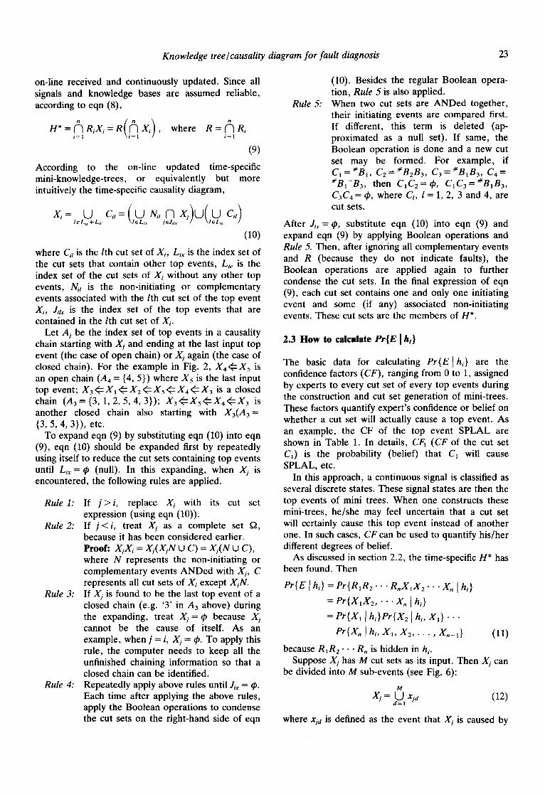
Suppose Xj has M cut sets as its input. Then Xj can be divided into M sub-events (see Fig. 6):

M

X j = U I Xjd (12)

where Xjd is defined as the event that Xj is caused by

24 Qin Zhang

Xll

XiM Fig. 6. Dividing X, into sub-events.

only the dth cut set. Let X = {Xi, X2 . . . . , Xj_1}. Then

er(Xj l X . , s2 , . . . , x j_, , hi}

=Pr{a~J=l X]dlX, hi}

=Pr{Ma~Jl XjdlX, hi}+ Pr{X/MlX, hi}

I GI } l } - Pr xj. IX, h, er Xj~, Ix, h,, U ~ . = d = l

:Pr{Ma~J_ixialX, hiI(1-Pr{XjMlX, hi, MaL2J=:xia})

+ Pr{xjM IX, h,} (13)

In eqn (13), since CjM is the only cause of x m,

Pr(x m IX, hi} = Pr(XjM I CjM, X, hi}Pr(CjM IX, hi} = Pr(XjM I CjM}Pr(CjM Ix, h,} = CFjMPr{CjM IX, hi} (14)

Similarly, let

we have

M - I U= U xj,t

d = l

M--I } er X~M IX, hi, U Xjd

d = l

= Pr(xjM Ix , h,, u )

= Pr(xj~ I G~,, x , h,, V}er (Cj~ IX, h,, V)

= P~(xjM I CjMIPr(GM IX, hi, V l

= CFjMPr{CjM IX, hl, U} Rule 6:

Rule 7:

(15)

When CjM is included in {X, hi}, Pr{G M IX, h,} = Pr{CjM IX, hi, U} = 1. When C m is exclusive with {X, hi} (i.e. CjM contains the fault events that are not included in hi which implies that hi is not the true fault cause, or GM contains the OK events that are exclusive with the

events in hi), Pr { CiM IX, hi) = Pr{CjM IX, h, U) = O.

Rule 8: When CjM is inclusive with but not included in {X, h;} (i.e. CjM contains top events that are not included in {X, hi}),

Pr{CjMIX, hi}=Prl( "] X, lX, hi } (16) I.l~.J M

Pr{CjMIX, hi, U}=Prl ~ XtlX, hi, U} I.l~J M

(17)

where JM is the index set of the top events contained in CjM but not in {X, h;}. Then eqn (11) is applied again to calculate eqns (16) and (17).

It is noted that the calculations for eqns (16) and (17) are exactly the same, because the condition U in eqn (17) have no effect on the calculation. For convenience, let Crm be the cut set encountered at any time during calculation of eqn (17) by applying eqn (11). If Cfm is included in or exclusive with {X, h;}, Cfm is independent of U conditioned by {X, hi} and Rules 6 and 7 will be applied. If Ci,,, is inclusive with but not included in {X, hi}, Rule 8 will be applied again. This process will continue until all top events are removed by applying Rules 6 and 7 or the last top event of a closed chain is reached and Rule 9 is applied. In such a way, the direct calculation of the influence of U on Cf,, is avoided. Therefore, eqn (13) can be simply written as

Pr{a~J_ I XjdlX, hi}

=er{MdLJ=ix/aIX, hi}(1--Pr{X]M[X, hi})

+ Pr{xjM IX, h,} (18)

without influencing the final result. In eqn (18), Pr{xjM IX, hi} is calculated by applying

Rules 7, 8 and 9. Thus,

is simplified as

Then by repeatedly applying eqn (18), Pr{EIhi} is calculated.

Rule 9: When Xi,,~ in Cr, ~ is the last top event of a closed chain identified during the calculation,

Pr{Cfm IX, hi} = Pr{Ci,m I X, h~, U} = 0 (18)

because Xp,, can not be the input of itself.


For the example in Fig. 3, when calculating Pr{X1 IX, hi}, XI~X2~XI is a closed chain. If X cannot break the chain (X does not contain X1 or X2), it must appear that xL~ is caused by CL~ = X2 and x2.~ is caused by C2.~ = Xt, which means that X1 is a cause of X~--an unreasonable loop. Thus, the last linkage X 2 ~ X I should be broken down. The consequence is the same as if Pr{C2.1 I X, hi} = O.

2.4 Spurious sensor signals and imperfect knowledge bases

It should be kept in mind that as n increases (more evidence added in), the hypothesis space H* becomes more and more small (more accurate). In some cases, it may appear that H * = 4, which means that no hypothesis can explain the appearance of these signals, or in other words, these signals are conflict.

The conflict signals may be caused by spurious sensor signals or imperfect knowledge bases. The spurious sensor signals may be caused by sensor failures, design errors and inappropriate sensor installations, etc. The imperfectness of knowledge bases is due to the lack of expert knowledge, errors during knowledge base construction or incorrect interpretation of signals.

In practice, it is very difficult to ensure the perfectness of the knowledge bases. For example, in the Three Mile Island accident, the high level of pressurizer was caused by the partial boiling in the primary loop under the low pressure caused by the failure to restore of a relief valve, rather than the malfunction of the high-pressure safety injection system. So the high level signal did not indicate the real amount of water in the primary loop and can be viewed as a spurious sensor signal. On the other hand, however, one may think that the signal is correct but the operators failed to correctly explain it, i.e. the operator's knowledge is imperfect. No matter what the reason is, the consequence is the same. The signals appear conflict and H* = q~.

When such cases appear, i.e. a null H* is reached, the received signals should be ignored one by one or one group by one group as suggested in eqn (5), until the non-null H* is reached. Since the mini-knowledge- bases are associated with signals, ignoring a signal means to ignore its associated mini-knowledge-base. So in our approach, the treatment to spurious sensor signals is the same as to imperfect knowledge bases.

Once a signal is ignored, the real state that the signal indicates remains unknown except that it is not as the signal indicates, or the cause of the signal is not as the mini-knowledge-base describes. In such cases, the procedures to find H* should be modified as follows.

First, ignore signals one by one or one group by one group. For each group, follow the procedures in

sections 2.2 and 2.3 and the modifications below to get Hgk, where H~k is the hypotheses given that the gth group of signals are ignored while there are k signals in this group.

Suppose Aj~c~k ej is the group of signals currently being ignored, where Ggk is the index set of signals to be ignored in group g while k is the number of signals to be ignored in the group, delete (i.e. ignore) f"lj~o~k ej from E.

When modifying the time-specific causality diagram or knowledge trees, all linkages associated with X# j ~ Ggk, remain as if they were all verified because the true state of signal j can be any.

In expanding eqn (10), the following rules are applied for Xj when j ~ Gg~.

Rule 10: If Xj is what ej indicates, let Xj= (complete set) because the true state of what ej indicates is unknown and can be caused by any event.

Rule 11: If Xj is not what ej indicates, substitute X) with its cut sets because what signal j indicates is unknown and can be any state including X i.

Rule 12: When calculating Pr{E l hi} , h i E Hg*k, if Xj is what ej indicates, Pr{XjIX, hi} = 1 because Xj = Q. Finally,

n - - l ckn

H*= ~, ~ Hg* k N S/ (19) k = l g = l j~Ggk

Pr{higk I E} = tr{higk l e} "~' ~ Pr{,,~, [E} k=l g=l

where

\ jeGRk

where C~ is the number of combinations of selecting k signals from n signals.

In some cases, the imperfectness of more than one mini-knowledge-bases is due to a common cause. In these cases, Pr{Nj ,c Sj} = max Pr{Sj) when calculating Pr{higk}. Jeg

The computation amount of above procedures are very large because of the combination explosion. But most likely, there is only one signal should be ignored. Then the combination explosion will not appear as described in section 2.2.

2.5 The treatment to unknown signals

It is possible in practice that for some reason, a group of signals are not received. This case is similar to that when a group of signals are spurious. A spurious

26 Qin Zhang

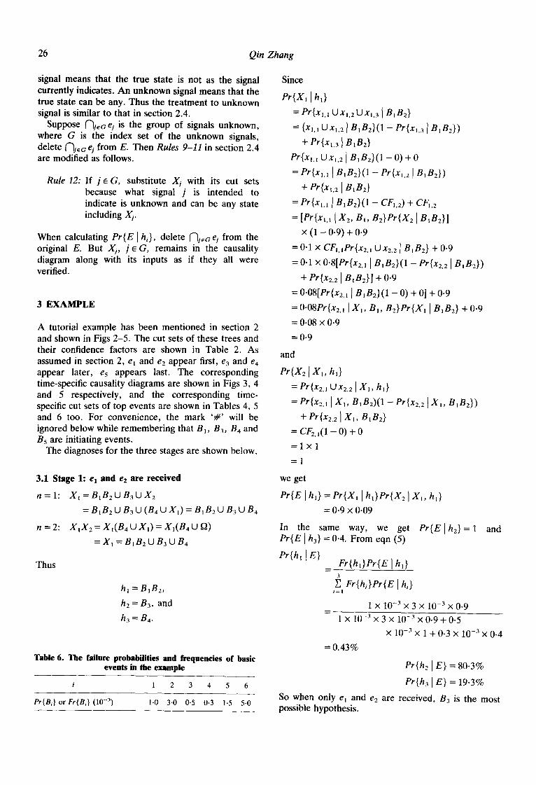
signal means that the true state is not as the signal currently indicates. An unknown signal means that the true state can be any. Thus the treatment to unknown signal is similar to that in section 2.4.

Suppose (']jEaej is the group of signals unknown, where G is the index set of the unknown signals, delete (']j~c ej from E. Then Rules 9-11 in section 2.4 are modified as follows.

Rule 12: If j • G, substitute Xj with its cut sets because what signal j is intended to indicate is unknown and can be any state including Xj.

When calculating Pr{E [ hi}, delete (-'ling ej from the original E. But Xj, j • G, remains in the causality diagram along with its inputs as if they all were verified.

3 E X A M P L E

A tutorial example has been mentioned in section 2 and shown in Figs 2-5. The cut sets of these trees and their confidence factors are shown in Table 2. As assumed in section 2, e, and e2 appear first, e 3 and e4 appear later, e5 appears last. The corresponding time-specific causality diagrams are shown in Figs 3, 4 and 5 respectively, and the corresponding time- specific cut sets of top events are shown in Tables 4, 5 and 6 too. For convenience, the mark 'CA' will be ignored below while remembering that B,, B3, B 4 and B5 are initiating events.

The diagnoses for the three stages are shown below.

3.1 Stage 1: el and e2 are rece ived

n = l : X,=BIB2UB31..JX2

= B,B2O B3U(B4U XI)= BIB2U B3U B4

n = 2: g i g 2 = X,(B4 U Xl) = g l (B4 I..J ~'2)

= X, = B,BzU B3U B4

Thus

hi = BIB2,

h2 = B3, and

h3 = B4.

Table 6. The failure probabilities and frequencies of basic events in the example

i 1 2 3 4 5 6

Pr{B~} or Fr{B~} (10 -3) 1"0 3.0 0.5 0.3 1.5 5-0

Since

Pr(X1 I hl}

= Pr{xl.l Uxl,2 UxL3 I BIB2}

= {XI,I UXI,2 I B ,B2}(1 -- Pr{x,,3 I B,B2})

+ er{x,.3 } B,BE}

Pr{x,,, Ux,.2 ] B,B2}(1 - 0) + 0

= Pr{x,,, I B,B2}(1 -Pr{x , .2 I B,BE})

+ er(x,.z { BtB2}

= Pr{xL, I BIB2}(1 - CFL2 ) + CFL2

= [Pr{x,,, I Xz, B,, Bz}Pr{X2 [ B,B2}I x (1 - 0.9) + 0.9

= 0.1 x CFl.lPr{x2.1 Uxz.21B,B2} + 0.9

=0.1 × 0.8[Pr{x2., I B,B2}(1 - Pr{x2.2 I B,B2))

+ Pr{x2.2 [ B,B2}] +0.9

= O.08[Pr{x2., [ B,B2}(1 - 0) + 01 + 0.9

= O.08Pr{x2,, IX, , B,, B2}Pr{X, I B,B2} + 0.9

= 0.08 x 0-9

=0-9

and

Pr{X2 IX, , h,}

= Pr{x2., Ux2.2 IX,, hi}

= Vr(x2., IX, , B,B2)(1 - Vr{x2.2 }X,, B,B2})

+ Pr{x2,2 IX1, B,B2)

= CF2.1(1 - 0) + 0

= 1 × 1

=1

we get

Pr{E I h,} = Pr{X, J h , }er{X 2 IX, , h,)

= 0.9 x 0.09

In the same way, we get Pr{E I h3} = 0.4. From eqn (5)

Pr h, I E}

Pr{EIh2 } = 1 and

Fr{h,}Pr{E l h,} 3

2 Fr{h,}Pr{EIh~ } i=1

1 x 10 .3 x 3 x 10 .3 x 0.9

1 x 10 -3 x 3 x 10 -3 × 0 .9 + 0-5

× 10 -3 × 1 + 0.3 x 10 -3 × 0.4

= 0.43%

Pr{h21 E} = 80.3%

Pr{h3 ]E) = 19.3%

So when only e, and e2 are received, B3 is the most possible hypothesis.


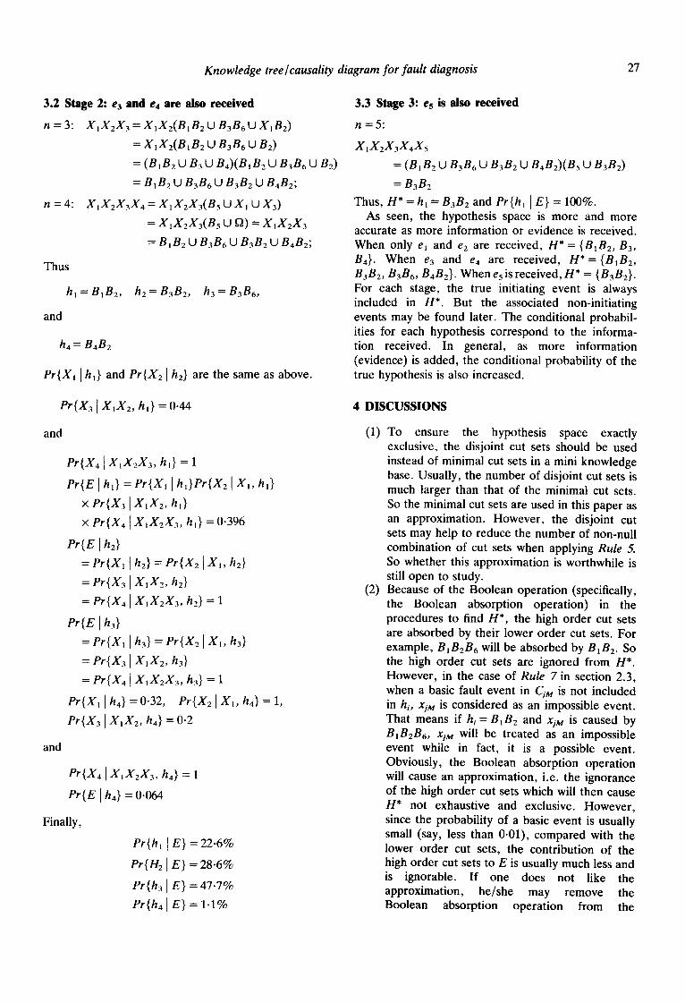
3.2 Stage 2:e3 and e4 are also received

n = 3: XIX2X3 = X I X z ( B 1 B 2 (-J B3B6 (-J X l B2)

= X I X z ( B I B 2 U B3B6 0 B2)

= (B,B2 U B3 LJ B4)(B,Bz U B3B6 U Be)

= BIB2 U B3B6 U B3B2 U B4B2;

n = 4: X 1 X 2 X 3 X 4 = X 1 X 2 X 3 ( B 5 U X I L.J X3)

= X I X 2 X 3 ( B 51.3 ~2) = S l X 2 g 3

= BIB2 U B3B6 U B3B2 U B4B2;

Thus

hi = B tB2 , h2 = B3Bz, h3 = B3B6,

and

h4 = B4B2

Pr{XJlhl} and Pr{X2lh2} are the same as above.

3.3 Stage 3: es is also received

n = 5 :

X l g 2 X 3 S 4 X 5

= ( B i B 2 U n 3 n 6 [..J n 3 n 2 [,.J n 4 n 2 ) ( n 5 [-J B3B2)

= B3B2

Thus, H* = hi = B3B2 and Pr{hl I E} = 100%. As seen, the hypothesis space is more and more

accurate as more information or evidence is received. When only el and e2 are received, H * = {BIB2, B3, B4}. When e3 and e4 are received, H*={BIB2, B3B2, B3B6, B4B2}. When e5 is received, H* = {B3B2}. For each stage, the true initiating event is always included in H*. But the associated non-initiating events may be found later. The conditional probabilities for each hypothesis correspond to the information received. In general, as more information (evidence) is added, the conditional probability of the true hypothesis is also increased.

Pr{X3 IX,X2, h,} = 0-44 4 DISCUSSIONS

and

and

Pr{g 4 [ XIX2X3, h,} = 1

Pr{E ]h,} = er{X, ] h,}er{Xz IX,, h,}

x Pr{X3 Ix,x2, h,}

x er{X4 } X,X2X3, hi} = 0.396

Pr{Elhz}

= Pr{Xl l h2} = Pr{X2 IX, , h2}

= Pr{X3IX,X2, h2}

= er{X4 I X,XeX3, h2) = 1

Pr{Elh3}

= Pr{X, I h3) = Pr{X2 l X,, h3)

= Pr(X3 I XIX2, h3} = P r { X 4 I X I X 2 X 3 , h3} = 1

e r { g I ] h4} -- 0.32, e r { X 2 ] X1, h4} = 1,

e r { X 3 [ SIX2, h4} -- 0-2

Pr{X4 I X l X 2 X 3 , h4} = 1

e r { E I h4} = 0.064

Finally,

Pr{h, I E} = 22.6%

Pr{H2 I E} = 28.6%

Pr{h3 I E} = 47.7%

e r { h 4 I E} --- 1.1%

(1)

(2)

To ensure the hypothesis space exactly exclusive, the disjoint cut sets should be used instead of minimal cut sets in a mini knowledge base. Usually, the number of disjoint cut sets is much larger than that of the minimal cut sets. So the minimal cut sets are used in this paper as an approximation. However, the disjoint cut sets may help to reduce the number of non-null combination of cut sets when applying Rule 5. So whether this approximation is worthwhile is still open to study. Because of the Boolean operation (specifically, the Boolean absorption operation) in the procedures to find H*, the high order cut sets are absorbed by their lower order cut sets. For example, B1BEB6 will be absorbed by B1B 2. So the high order cut sets are ignored from H*. However, in the case of Rule 7 in section 2.3, when a basic fault event in CjM is not included in hi, XjM is considered as an impossible event. That means if h~--B1B 2 and xjM is caused by B1BEB6, XjM will be treated as an impossible event while in fact, it is a possible event. Obviously, the Boolean absorption operation will cause an approximation, i.e. the ignorance of the high order cut sets which will then cause H* not exhaustive and exclusive. However, since the probability of a basic event is usually small (say, less than 0-01), compared with the lower order cut sets, the contribution of the high order cut sets to E is usually much less and is ignorable. If one does not like the approximation, he/she may remove the Boolean absorption operation from the

28 Qin Zhang

Boolean operation during finding H*. But the computation amount will be larger.

(3) In this approach, we do not use the number such as Pr{Bj} in calculating Pr{EIhi}. So the restriction of Bayesian theory mentioned in section 1 is avoided.

(4) Since the diagnosis is divided into two steps: first find H* and then calculate Pr{hiIE}, the computation is greatly simplified because one does not have to calculate Pr{hilE} for the whole H (which is much larger than H*) and then use Pr{hilE } to describe H*. Moreover , the computation amount in this approach is proportional to the size of the problem and will not increase exponentially as the increase of loops, because a loop is only a closed chain, and the treatment to a closed chain is almost the same as to an open chain.

REFERENCES

1. Kim, I. S., Modarres, M. & Hunt, R. N. M., A model-based approach to on-line process disturbance

management: the models. Reliability Engng System Safety, 28 (1990) 265-305.

2. Chung, D. T., Modarres, M. & Hunt, R. N. M., GOTRES: an expert system for fault detection and analysis. Reliability Engng System Safety, 24 (1989) 113-37.

3. Nelson, W. R., REACTOR: an expert system for diagnosis and treatment of nuclear reactor accidents. Proc. AAAI, 82 (1982) 296-301.

4. Kaplan, S., Frank, M. V., Bley, D. C. & Lindsay, D. G., Outline of COPILOT, an expert system for reactor operational assistance, using a Bayesian diagnostic model. Reliability Engng System Safety, 22 (1988) 411-40.

5. Pearl, J., Fusion, propagation, and structuring in belief networks. Artificial Intelligence, 29 (1986) 241-88.

6. Shortliffe, E. H., A model of inexact reasoning in medicine. Mathem. Biosci., 23 (1975) 351-79.

7. Shafer, G., A Mathematical Theory of Evidence. Princeton University Press, USA, 1976.

8. Zadeh, L. A., The role of fuzzy logic in the management of uncertainty in expert systems. Fuzzy Sets and Systems, 11 (1983) 199-227.

9. Zhang, Q., Okrent, D. & Apostolakis, G. E., An expert system approach for fault diagnosis to cope with spurious sensor signals and process state uncertainty. Reliability Engng System Safety, (1991) 121-42.

Documents

A frequency and knowledge tree/causality diagram based expert system approach for fault diagnosis