A length-based hierarchical model of brown trout (Salmo trutta fario) growth and production

A length-based hierarchical model of brown trout (Salmo truttafario) growth and production

Jean-Baptiste Lecomte1,2 and Christophe Laplanche�,1,2

1 Universite de Toulouse; INP, UPS, EcoLab (Laboratoire Ecologie Fonctionnelle

et Environnement); ENSAT, Avenue de l’Agrobiopole, 31326 Castanet Tolosan, France2 CNRS, EcoLab, 31326 Castanet Tolosan, France

Received 7 April 2011, revised 1 September 2011, accepted 9 September 2011

We present a hierarchical Bayesian model (HBM) to estimate the growth parameters, production,and production over biomass ratio (P/B) of resident brown trout (Salmo trutta fario) populations.The data which are required to run the model are removal sampling and air temperature data whichare conveniently gathered by freshwater biologists. The model is the combination of eight submodels:abundance, weight, biomass, growth, growth rate, time of emergence, water temperature, and pro-duction. Abundance is modeled as a mixture of Gaussian cohorts; cohorts centers and standarddeviations are related by a von Bertalanffy growth function; time of emergence and growth rate arefunctions of water temperature; water temperature is predicted from air temperature; biomass,production, and P/B are subsequently computed. We illustrate the capabilities of the model byinvestigating the growth and production of a brown trout population (Neste d’Oueil, Pyrenees,France) by using data collected in the field from 2005 to 2010.

Keywords: Growth; Hierarchical Bayesian model; Production; Removal sampling; Salmotrutta.

Supporting Information for this article is available from the author or on the WWW underhttp://dx.doi.org/10.1002/bimj.201100083

1 Introduction

In order to evaluate, compare, and predict the status of fish populations, freshwater biologists haveconsidered numerous descriptors of fish populations. Such variables can characterize fish stocks(Pauly and Moreau 1997; Kwak and Waters 1997; Ruiz and Laplanche 2010) duration and rates ofsuccess through life-history stages (Hutchings 2002, Klemetsen et al., 2003), phenotypic or geno-typic traits (Ward, 2002; Shinn, 2010). Descriptors of fish populations can be examined separately,depending on the population aspect under focus. For instance, the impact of surface water con-tamination by pesticides on fish can be investigated by assessing DNA damage to blood cells(Polard et al., 2011). Aquatic resource management would rather focus on fish stock variables, suchas abundance (number of fish per unit area of stream), biomass (mass of fish per unit area),production (mass of fish produced per unit area per unit time), or production over biomass ratioP/B (Pauly and Moreau, 1997). The drawback of examining a single population variable is itslimited, descriptive prospect. A countermeasure would be to relate a population variable to cov-ariates, e.g. environmental variables or descriptors of coexisting populations. As an illustration,growth of salmonids has been related to environmental factors such as temperature (Mallet et al.,

*Corresponding author: e-mail: [email protected], Tel: 133-534-323-973, Fax: 133-534-323-901

r 2011 WILEY-VCH Verlag GmbH & Co. KGaA, Weinheim

108 Biometrical Journal 54 (2012) 1, 108–126 DOI: 10.1002/bimj.201100083

1999) and stream flow (Jensen and Johnsen 1999; Daufresne and Renault, 2006). Descriptors of apopulation can also be examined jointly. The examination of multiple variables has a more potent,explicative prospect and could improve our understanding of population dynamics (Nordwall et al.2001).

Brown trout (Salmo trutta) is indigenous to Eurasia. Brown trout has been introduced to non-Eurasian freshwaters for fishing purposes. It can either grow in oceans and migrate to freshwatersfor reproduction (S. trutta trutta), or live in lakes (S. trutta lacustris), or be stream-resident (S. truttafario). As a result of such adaptation capabilities, brown trout has successfully colonized fresh-waters to a world-wide distribution (Elliott, 1994; Klemetsen et al., 2003). Although ecologicallyvariable, brown trout is demanding in terms of habitat and water quality. As a result, brown trout isa relevant bioindicator of the quality of freshwaters at a global scale (Lagadic et al 1998; Wood2007). Moreover, a fundamental environmental variable driving brown trout life history is tem-perature (Jonsson and Jonsson, 2009), hence using brown trout as a bioindicator of climate change.Temperature affects growth (as aforementioned) as well as life-stage timing (Webb and McLay,1996; Armstrong et al., 2003). Key life-stages of brown trout are egg laying (oviposition), hatchingof larvae, emergence of fry, reproduction of adults, and death. In our case, we will focus on theeffect of temperature on growth and on time between oviposition and emergence of riverine browntrout (S. trutta fario). We will also consider several variables characterizing stocks (abundance,biomass, production).

Abundance of riverine fish species is conveniently assessed through removal sampling: (i) a reach isspatially delimited (later referred to as a stream section), (ii) fractions of fish are successively removedof the section by electrofishing and counted, (iii) captured fish are released altogether (Lobon-Cervia,1991). Abundance is typically computed by using the method suggested by Carle and Strub (1978): themain statistical assumption was that the probability of capturing fish (referred to in the following ascatchability) would be equal for all fish. Some contributions have shown, however, that the use ofmore advanced statistical models is recommendable in the aim of lowering estimation bias (Petersonet al., 2004; Riley and Fausch, 1992). The trend is to construct such statistical models within aBayesian framework (Congdon, 2006). Recent hierarchical Bayesian models (HBMs) relate abun-dance to environmental covariates (Rivot et al., 2008; Ebersole et al., 2009), include heterogeneity ofthe catchability (Mantyniemi et al., 2005; Do-razio et al., 2005; Ruiz and Laplanche, 2010), and canhandle multiple sampling stream sections (Wyatt, 2002; Webster et al., 2008; Laplanche, 2010). Thereason of popularity of HBMs over the last decade is their ability to handle complex relationships(multi-level, non-linear, mixed-effect) between variables with heterogeneous sources (relationships,data, priors) of knowledge. Freshwater biologists can statistically relate multiple descriptors of fishpopulations together with covariates within a single HBM framework.

We present an HBM of riverine brown trout growth and production. Our primary objective is toprovide a layout to compute growth parameters of brown trout populations by using accessible data(namely removal sampling and air temperature data). Our second objective is to use such a layout tocompute interval estimates of brown trout production. To fulfill the first objective, we extend theabundance model of Ruiz and Laplanche (2010) with a growth module. The abundance modelperforms a multimodal decomposition of length-abundance plots. Our growth module constrainsparameters of the multimodal decomposition with a growth function. The interest is twofold: toguide the decomposition of length-abundance plots with a growth function and to use length-abundance plots to estimate growth parameters. Ruiz and Laplanche (2010) also created a modulewhich computes fish biomass. To fulfill the second objective, we extend their biomass module with aproduction model. The overall model is the combination of eight HBMs, three (abundance, weight,biomass) related to the contribution of Ruiz and Laplanche (2010) and five to growth and pro-duction (growth, growth rate, emergence, temperature, production), which are presented succes-sively. We show the capability of the overall model to estimate the growth parameters and theproduction of a brown trout population with a data set collected in the field. We discuss possibleextensions of the current model.

Biometrical Journal 54 (2012) 1 109

r 2011 WILEY-VCH Verlag GmbH & Co. KGaA, Weinheim www.biometrical-journal.com

2 Materials and methods

2.1 Notations and measured variables

A single section (of area A, m2) of a stream populated with S. trutta fario is sampled by electrofishing.Electrofishing is spread over several years in a series of O campaigns with Jo removals per campaign(index over campaigns is o 2 f1; . . . ;Og). The number of campaign(s) per year as well as the number ofremoval(s) per campaign can be variable. Time scale is daily, spans from January 1st of the year of thefirst campaign to December 31st of the year of the last campaign, with a total of T days. Times ofcampaigns are noted to (day). Let Co;j be the number of fish caught during removal j 2 f1; . . . ; Jog attime to and Co ¼

Pj Co;j be the total number of fish caught at time to. The length and weight of the

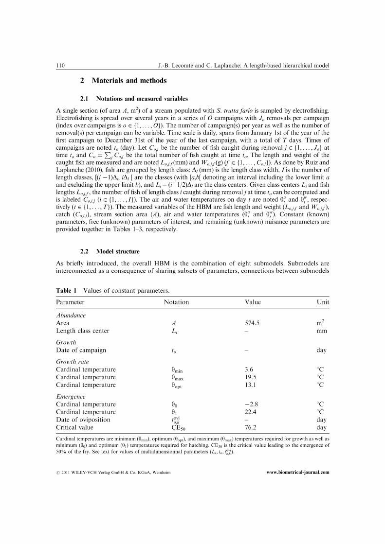
caught fish are measured and are noted Lo;j;f (mm) andWo;j;f (g) (f 2 f1; . . . ;Co;jg). As done by Ruiz andLaplanche (2010), fish are grouped by length class: Dl (mm) is the length class width, I is the number oflength classes, [(i �1)Dl, iDl [ are the classes (with [a,b[ denoting an interval including the lower limit aand excluding the upper limit b), and Li5 (i�1/2)Dl are the class centers. Given class centers Li and fishlengths Lo;j;f , the number of fish of length class i caught during removal j at time to can be computed andis labeled Co;i;j (i 2 f1; . . . ; Ig). The air and water temperatures on day t are noted yat and ywt , respec-tively (t 2 f1; . . . ;Tg). The measured variables of the HBM are fish length and weight (Lo;j;f andWo;j;f ),catch (Co;i;j), stream section area (A), air and water temperatures (yat and ywt ). Constant (known)parameters, free (unknown) parameters of interest, and remaining (unknown) nuisance parameters areprovided together in Tables 1–3, respectively.

2.2 Model structure

As briefly introduced, the overall HBM is the combination of eight submodels. Submodels areinterconnected as a consequence of sharing subsets of parameters, connections between submodels

Table 1 Values of constant parameters.

Parameter Notation Value Unit

AbundanceArea A 574.5 m2

Length class center Li – mm

GrowthDate of campaign to – day

Growth rateCardinal temperature ymin 3.6 1CCardinal temperature ymax 19.5 1CCardinal temperature yopt 13.1 1C

EmergenceCardinal temperature y0 �2.8 1CCardinal temperature y1 22.4 1CDate of oviposition tovio;k – dayCritical value CE50 76.2 day

Cardinal temperatures are minimum (ymin), optimum (yopt), and maximum (ymax) temperatures required for growth as well as

minimum (y0) and optimum (y1) temperatures required for hatching. CE50 is the critical value leading to the emergence of

50% of the fry. See text for values of multidimensionnal parameters (Li; to; tovio;k).

110 J.-B. Lecomte and C. Laplanche: A length-based hierarchical model


are illustrated in Fig. 1: abundance and growth submodels depend on common parameters (mo;k andso;k, defined later), growth depends on the time of emergence and growth rate, these quantitiesfurther depend on the water temperature, fish biomass is the cross-product of fish weight andabundance, and the combination of growth and biomass parameters lead to production. Submodelsare also connected to subsets of measured variables: Fish weight (Wo;j;f ) is predicted from fish length(Lo;j;f ), water temperature (ywt ) is predicted from air temperature (yat ), and abundance is related toremoval sampling catch (Co;i;j) plus stream section area (A). The model is structured into five levels :campaign (o 2 f1; . . . ;Og), day (t 2 f1; . . . ;Tg), length class (i 2 f1; . . . ; Ig), removal (j 2 f1; . . . ; Jog),plus an additional level, cohort (k 2 f1; . . . ;Kg), which is defined later. The temperature submodel isdealt with in Appendix A (Supporting Infomation), remaining submodels are successively presentedbelow.

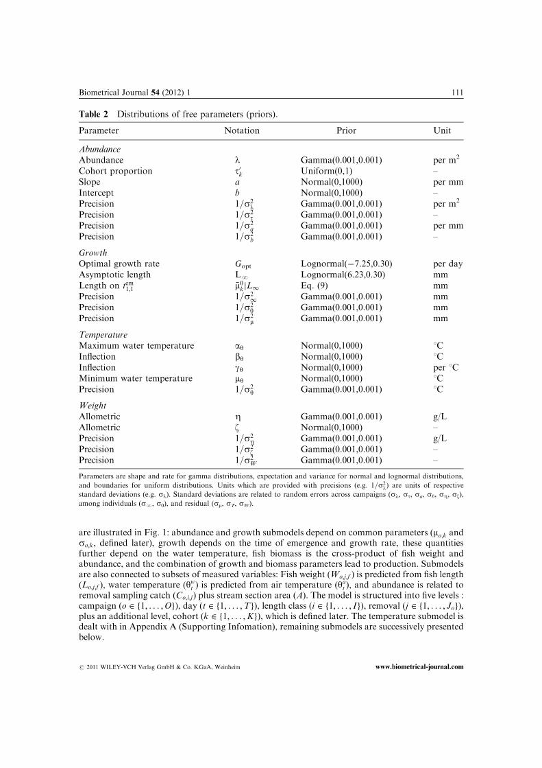
Table 2 Distributions of free parameters (priors).

Parameter Notation Prior Unit

AbundanceAbundance l Gamma(0.001,0.001) per m2

Cohort proportion t0k Uniform(0,1) –Slope a Normal(0,1000) per mmIntercept b Normal(0,1000) –Precision 1=s2

l Gamma(0.001,0.001) per m2

Precision 1=s2t Gamma(0.001,0.001) –

Precision 1=s2a Gamma(0.001,0.001) per mm

Precision 1=s2b Gamma(0.001,0.001) –

GrowthOptimal growth rate Gopt Lognormal(�7.25,0.30) per dayAsymptotic length LN Lognormal(6.23,0.30) mmLength on tem1;1 �m0kjL1 Eq. (9) mmPrecision 1=s2

1 Gamma(0.001,0.001) mmPrecision 1=s2

0 Gamma(0.001,0.001) mmPrecision 1=s2

m Gamma(0.001,0.001) mm

TemperatureMaximum water temperature ay Normal(0,1000) 1CInflection by Normal(0,1000) 1CInflection gy Normal(0,1000) per 1CMinimum water temperature my Normal(0,1000) 1CPrecision 1=s2

y Gamma(0.001,0.001) 1C

WeightAllometric Z Gamma(0.001,0.001) g/LAllometric z Normal(0,1000) –Precision 1=s2

Z Gamma(0.001,0.001) g/LPrecision 1=s2

z Gamma(0.001,0.001) –Precision 1=s2

W Gamma(0.001,0.001) –

Parameters are shape and rate for gamma distributions, expectation and variance for normal and lognormal distributions,

and boundaries for uniform distributions. Units which are provided with precisions (e.g. 1=s2l) are units of respective

standard deviations (e.g. sl). Standard deviations are related to random errors across campaigns (sl, st, sa, sb, sZ, sz),

among individuals (sN, s0), and residual (sm, sT, sW).



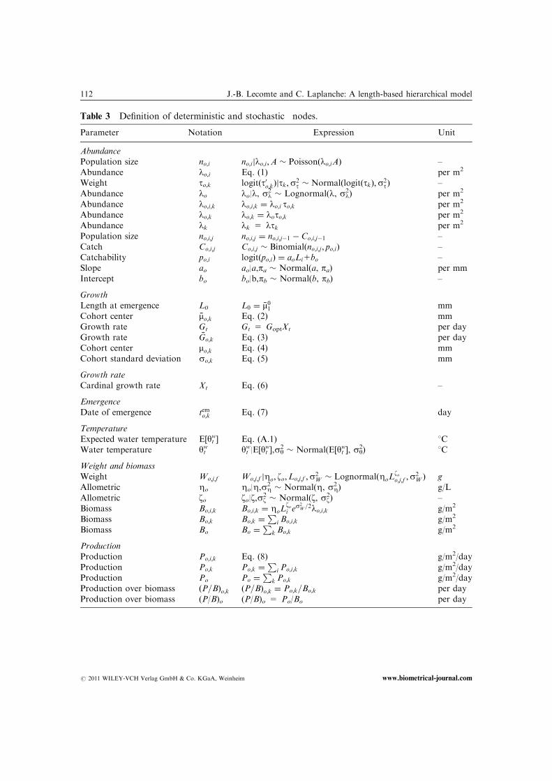
Table 3 Definition of deterministic and stochastic� nodes.

Parameter Notation Expression Unit

Abundance

Population size� no;i no;ijlo;i;A � Poissonðlo;iAÞ –

Abundance lo;i Eq. (1) per m2

Weight to;k logitðt0o;kÞjtk;s2t � NormalðlogitðtkÞ;s2

tÞ –

Abundance� lo lo|l, sl2� Lognormal(l, sl

2) per m2

Abundance lo;i;k lo;i;k ¼ lo;i to;k per m2

Abundance lo;k lo;k ¼ loto;k per m2

Abundance lk lk 5 ltk per m2

Population size no;i;j no;i;j ¼ no;i;j�1 � Co;i;j�1 –

Catch� Co;i;j Co;i;j � Binomialðno;i;j ; po;iÞ –

Catchability po;i logitðpo;iÞ ¼ aoLi1bo –

Slope� ao ao|a,pa � Normal(a, pa) per mm

Intercept� bo bo|b,pb � Normal(b, pb) –

Growth

Length at emergence L0 L0 ¼ �m01 mm

Cohort center �mo;k Eq. (2) mm

Growth rate Gt Gt 5 GoptXt per day

Growth rate �Go;k Eq. (3) per day

Cohort center� mo;k Eq. (4) mm

Cohort standard deviation so;k Eq. (5) mm

Growth rate

Cardinal growth rate Xt Eq. (6) –

Emergence

Date of emergence temo;k Eq. (7) day

Temperature

Expected water temperature E[ytw] Eq. (A.1) 1C

Water temperature� ytw yt

w|E[ytw],sy

2� Normal(E[yt

w], sy2) 1C

Weight and biomass

Weight� Wo;j;f Wo;j;f jZo; zo;Lo;j;f ;s2W � LognormalðZoL

zoo;j;f ;s

2W Þ g

Allometric� Zo Zo|Z,sZ2� Normal(Z, sZ

2 ) g/L

Allometric� zo zo|z,sz2� Normal(z, sz

2) –

Biomass Bo;i;k Bo;i;k ¼ ZoLzoi e

s2W=2lo;i;k g/m2

Biomass Bo;k Bo;k ¼P

i Bo;i;k g/m2

Biomass Bo Bo ¼P

k Bo;k g/m2

Production

Production Po;i;k Eq. (8) g/m2/day

Production Po;k Po;k ¼P

i Po;i;k g/m2/day

Production Po Po ¼P

k Po;k g/m2/day

Production over biomass ðP=BÞo;k ðP=BÞo;k ¼ Po;k=Bo;k per day

Production over biomass (P/B)o (P/B)o 5 Po/Bo per day



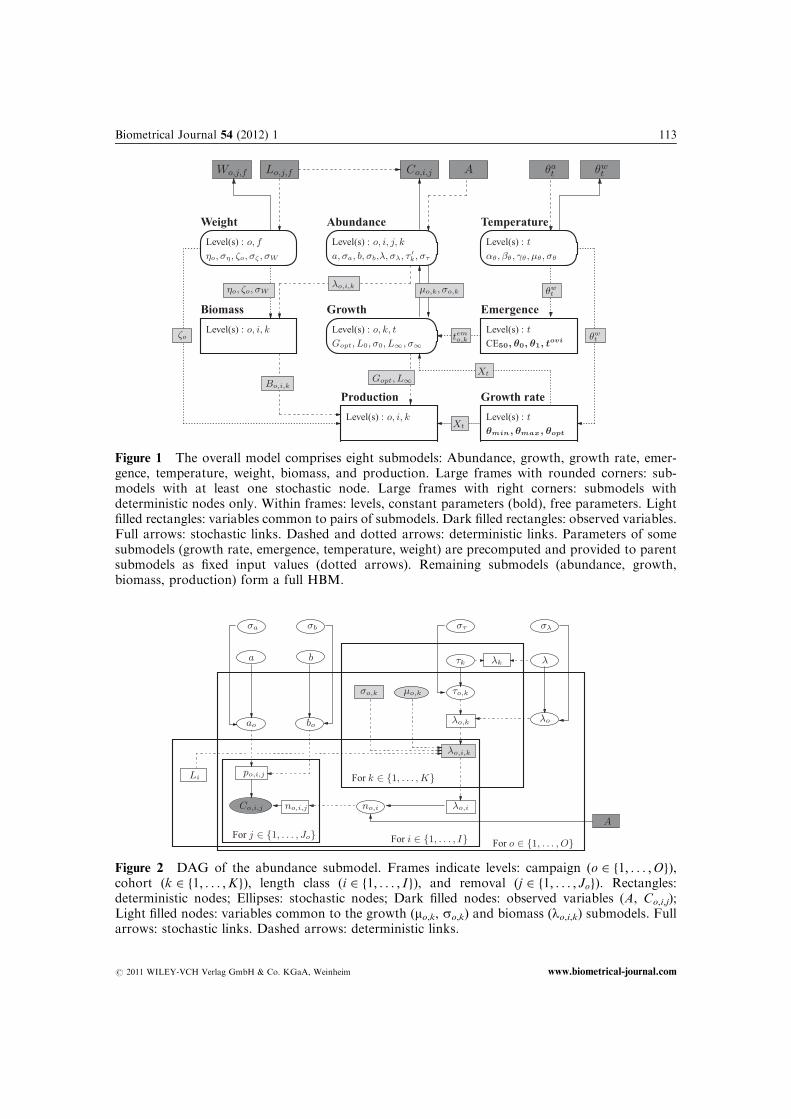
Figure 1 The overall model comprises eight submodels: Abundance, growth, growth rate, emer-gence, temperature, weight, biomass, and production. Large frames with rounded corners: sub-models with at least one stochastic node. Large frames with right corners: submodels withdeterministic nodes only. Within frames: levels, constant parameters (bold), free parameters. Lightfilled rectangles: variables common to pairs of submodels. Dark filled rectangles: observed variables.Full arrows: stochastic links. Dashed and dotted arrows: deterministic links. Parameters of somesubmodels (growth rate, emergence, temperature, weight) are precomputed and provided to parentsubmodels as fixed input values (dotted arrows). Remaining submodels (abundance, growth,biomass, production) form a full HBM.

Figure 2 DAG of the abundance submodel. Frames indicate levels: campaign (o 2 f1; . . . ;Og),cohort (k 2 f1; . . . ;Kg), length class (i 2 f1; . . . ; Ig), and removal (j 2 f1; . . . ; Jog). Rectangles:deterministic nodes; Ellipses: stochastic nodes; Dark filled nodes: observed variables (A, Co,i,j);Light filled nodes: variables common to the growth (mo,k, so,k) and biomass (lo,i,k) submodels. Fullarrows: stochastic links. Dashed arrows: deterministic links.



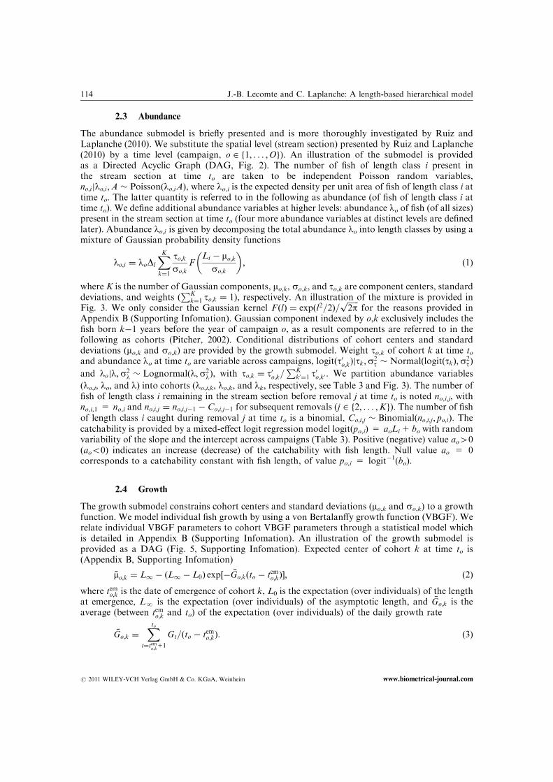
2.3 Abundance

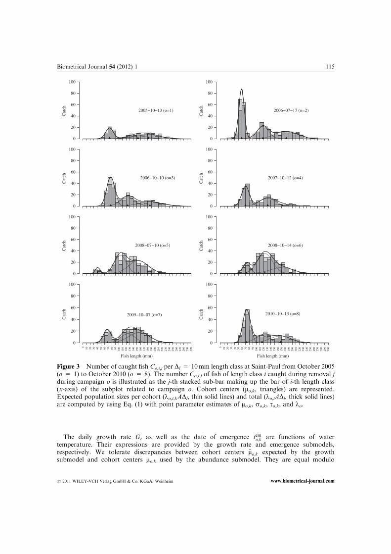
The abundance submodel is briefly presented and is more thoroughly investigated by Ruiz andLaplanche (2010). We substitute the spatial level (stream section) presented by Ruiz and Laplanche(2010) by a time level (campaign, o 2 f1; . . . ;Og). An illustration of the submodel is providedas a Directed Acyclic Graph (DAG, Fig. 2). The number of fish of length class i present inthe stream section at time to are taken to be independent Poisson random variables,no;ijlo;i;A � Poissonðlo;iAÞ, where lo,i is the expected density per unit area of fish of length class i attime to. The latter quantity is referred to in the following as abundance (of fish of length class i attime to). We define additional abundance variables at higher levels: abundance lo of fish (of all sizes)present in the stream section at time to (four more abundance variables at distinct levels are definedlater). Abundance lo;i is given by decomposing the total abundance lo into length classes by using amixture of Gaussian probability density functions

lo;i ¼ loDl

XKk¼1

to;kso;k

FLi � mo;k

so;k

� �; ð1Þ

where K is the number of Gaussian components, mo,k, so,k, and to,k are component centers, standarddeviations, and weights (

PKk¼1 to;k ¼ 1), respectively. An illustration of the mixture is provided in

Fig. 3. We only consider the Gaussian kernel FðlÞ ¼ expðl2=2Þ=ffiffiffiffiffiffi2pp

for the reasons provided inAppendix B (Supporting Infomation). Gaussian component indexed by o,k exclusively includes thefish born k�1 years before the year of campaign o, as a result components are referred to in thefollowing as cohorts (Pitcher, 2002). Conditional distributions of cohort centers and standarddeviations (mo,k and so,k) are provided by the growth submodel. Weight to,k of cohort k at time toand abundance lo at time to are variable across campaigns, logitðt0o;kÞjtk;s

2t � NormalðlogitðtkÞ;s2

tÞ

and lojl;s2l � Lognormalðl;s2

lÞ, with to;k ¼ t0o;k=PK

k0¼1 t0o;k0 . We partition abundance variables

(lo,i, lo, and l) into cohorts (lo,i,k, lo,k, and lk, respectively, see Table 3 and Fig. 3). The number offish of length class i remaining in the stream section before removal j at time to is noted no,i,j, withno,i,1 5 no,i and no;i;j ¼ no;i;j�1 � Co;i;j�1 for subsequent removals (j 2 f2; . . . ;Kg). The number of fishof length class i caught during removal j at time to is a binomial, Co;i;j � Binomialðno;i;j ; po;iÞ. Thecatchability is provided by a mixed-effect logit regression model logit(po,i) 5 aoLi 1 bo with randomvariability of the slope and the intercept across campaigns (Table 3). Positive (negative) value ao40(aoo0) indicates an increase (decrease) of the catchability with fish length. Null value ao 5 0corresponds to a catchability constant with fish length, of value po,i 5 logit�1(bo).

2.4 Growth

The growth submodel constrains cohort centers and standard deviations (mo,k and so,k) to a growthfunction. We model individual fish growth by using a von Bertalanffy growth function (VBGF). Werelate individual VBGF parameters to cohort VBGF parameters through a statistical model whichis detailed in Appendix B (Supporting Infomation). An illustration of the growth submodel isprovided as a DAG (Fig. 5, Supporting Infomation). Expected center of cohort k at time to is(Appendix B, Supporting Infomation)

�mo;k ¼ L1 � ðL1 � L0Þ exp½� �Go;kðto � temo;kÞ�; ð2Þ

where temo;k is the date of emergence of cohort k, L0 is the expectation (over individuals) of the lengthat emergence, LN is the expectation (over individuals) of the asymptotic length, and �Go;k is theaverage (between temo;k and to) of the expectation (over individuals) of the daily growth rate

�Go;k ¼Xto

t¼temo;k

11

Gt=ðto � temo;kÞ: ð3Þ



The daily growth rate Gt as well as the date of emergence temo;k are functions of watertemperature. Their expressions are provided by the growth rate and emergence submodels,respectively. We tolerate discrepancies between cohort centers �mo;k expected by the growthsubmodel and cohort centers mo,k used by the abundance submodel. They are equal modulo

Cat

ch

0

20

40

60

80

100

2005−10−13 (o=1)

Cat

ch

0

20

40

60

80

100

2006−07−17 (o=2)

Cat

ch

0

20

40

60

80

100

2006−10−10 (o=3)

Cat

ch0

20

40

60

80

100

2007−10−12 (o=4)

Cat

ch

0

20

40

60

80

100

2008−07−10 (o=5)

Cat

ch

0

20

40

60

80

100

2008−10−14 (o=6)

Fish length (mm)

Cat

ch

0

20

40

60

80

100

0 10 20 30 40 50 60 70 80 90 100

110

120

130

140

150

160

170

180

190

200

210

220

230

240

250

260

270

280

290

300

2009−10−07 (o=7)

Fish length (mm)

Cat

ch

0

20

40

60

80

100

0 10 20 30 40 50 60 70 80 90 100

110

120

130

140

150

160

170

180

190

200

210

220

230

240

250

260

270

280

290

300

2010−10−13 (o=8)

Figure 3 Number of caught fish Co,i,j per Dl 5 10mm length class at Saint-Paul from October 2005(o 5 1) to October 2010 (o 5 8). The number Co,i,j of fish of length class i caught during removal jduring campaign o is illustrated as the j-th stacked sub-bar making up the bar of i-th length class(x-axis) of the subplot related to campaign o. Cohort centers (mo,k, triangles) are represented.Expected population sizes per cohort (lo,i,kADl, thin solid lines) and total (lo,iADl, thick solid lines)are computed by using Eq. (1) with point parameter estimates of mo,k, so,k, to,k, and lo.



a logit-transformed residual normal error

logitmo;k � �m0o;k�m1o;k � �m0o;k

!j �mo;k; �m

0o;k; �m

1o;k;s

2m � Normal logit

�mo;k � �m0o;k�m1o;k � �m0o;k

!;s2

m

!; ð4Þ

of variance s2m, where �m

0o;k is the center of cohort k at the date of emergence of the year of campaign

o (temo;1) and �m1o;k is the center of cohort k at the end of the year of campaign o (December 31th). The

motivation to include this additional error term in the model is illustrated and discussed later.Variables �m0o;k and �m1o;k are computed with a formula similar to Eq. (2). The scaled logit transfor-mation of Eq. (4) ensures that both �mo;k and mo;k are greater than �m0o;k and lesser than �m1o;k. Thestandard deviation so,k is provided by

s2o;k ¼ s2

0

½L1 � �mo;k�2

½L1 � L0�2

1s21

½ �mo;k � L0�2

½L1 � L0�2; ð5Þ

where s0 and sN are the standard deviations representative of variability among individuals of thelength at emergence and of the asymptotic length, respectively (Appendix B, Supporting Infoma-tion). We do not model growth of fish born before the year of the first campaign. The resulting edgeeffects are dealt with by simulating growth by starting on the date of emergence on the year of thefirst campaign (tem1;1). Cohort centers on such a date are labeled �m0k.

2.5 Growth rate and emergence

2.5.1 Growth rateWater temperature affects fish growth (Jonsson and Jonsson, 2009). Therefore, various authorshave included seasonal variability in the VBGF parameters to consider the effects of water tem-perature on growth (Taylor, 1960; Somers, 1988; Mallet et al., 1999). Fontoura and Agostinho(1996) have successfully modeled the growth of two freshwater fish species by using the VBGF witha growth rate as a deterministic function of water temperature. The latter authors have suggestedthe use of a bell-shaped relationship between temperature and growth rate, with a null growth ratebelow a minimum temperature (ymin) or above a maximum temperature (ymax) and a maximumgrowth rate at an optimum temperature (yopt). Mallet et al. (1999) have suggested a similarrelationship to predict fish growth rate from water temperature. The latter relationship originatesfrom the work of Rosso et al. (1995) dealing with bacterial growth with pH. We use the relationshipprovided by Mallet et al. (1999) to relate daily growth rate to water temperature. The daily growthrate is Gt 5 GoptXt where Gopt is the growth rate at optimum temperature yopt and Xt is the cardinaldaily growth rate

Xt ¼ðywt � yminÞðy

wt � ymaxÞ

ðywt � yminÞðywt � ymaxÞ � ðy

wt � yoptÞ

2; ð6Þ

where ywt is the water temperature at time t.

2.5.2 EmergenceWater temperature affects life-stage timing of fish (Jonsson and Jonsson, 2009). Time from ovi-position to hatching and time from hatching to emergence are related to water temperature (Webband McLay, 1996; Armstrong et al., 2003). Elliott and Hurley (1998) have shown that the delaybetween oviposition tovi and the median date of emergence tem (date when half fry have emerged) of

brown trout can be well-predicted by finding tem leading toR temtoviðywðtÞ � y0Þ=½y1 � ywðtÞ�dt ¼ CE50,

where yw(t) is water temperature at time t, y0 is the minimum temperature required for hatching, y1is the optimum temperature for hatching, and CE50 is the critical value leading to the emergence of50% of the fry. By approximating the latter integral by the midpoint rule with a daily time step, the



date of emergence temo;k of fish which are present under the form of cohort k at time to leads to

Xtemo;kt¼tovi

o;k

ywt � y0y1 � ywt

’ CE50: ð7Þ

2.6 Weight

Length and weight of fish f 2 f1; . . . ;Co;jg caught during removal j at time to are related by the

allometric formula Wo;j;f ¼ ZoLzoo;j;f expðeo;j;f Þ with an i.i.d lognormal residual error of variance s2

W ,

eo;j;f js2W � Normalð0;s2

W Þ. Allometric parameters Zo and zo are allowed to vary between campaignsand are taken independent (Table 3). Log-transformed, the latter submodel is a two-level linearmixed-effect model with a normal, heteroscedastic residual error (Pinheiro and Bates, 2000).

2.7 Model outputs: Biomass and production

The biomass of fish of length class i of cohort k at time to is approximately Bo;i;k ’ ZoLzoi e

s2W=2lo;i;k

(Ruiz and Laplanche 2010). The biomass of fish of cohort k at time to is Bo;k ¼P

i Bo;i;k and theoverall biomass at time to is Bo ¼

Pk Bo;k. The production of fish of length class i of cohort k at time

to is

Po;i;k ¼dBo;i;k

dt¼ zo

Bo;i;k

Li

dLi

dt¼ zoBo;i;kGo

L1 � Li

Li; ð8Þ

where Go 5 Gt for t 5 to. The production of fish of cohort k at time to is Po;k ¼ dBo;k=dt ¼P

i Po;i;k

and the overall production at time to is Po ¼ dBo=dt ¼P

k Po;k. Respective production over bio-mass ratios are (P/B)o,k 5 Po,k/Bo,k and (P/B)o 5 Po/Bo.

2.8 Constant parameters, data sets, and priors

2.8.1 Constant parametersWe use cardinal temperatures (ymin, ymax, yopt) suggested by Elliott et al. (1995) for S. trutta fario.Dates of emergence are computed from Eq. (7) by using parameter values (y0, y1, CE50) provided byElliott and Hurley (1998) for S. trutta. Oviposition dates are assumed equal for all years (October20th). Values of constant parameters are provided in Table 1 and are highlighted in Fig. 1.

2.8.2 Data setsWe use the model to study growth and production of resident brown trout (S. trutta fario) popu-lating the Neste d’Oueil stream (Haute Garonne, Pyrenees, France). Neste d’Oueil brown trouts arethe dominant species of the stream (Gouraud et al., 2001). Trouts which are considered in this casestudy were electrofished at a single stream section (Saint-Paul d’Oueil) O5 8 times from 2005 to2010, 6 times in October (13th, 10th, 12th, 14th, 7th, and 13th from 2005 to 2010, respectively) plustwice in July (2006 July 17th, 2008 July 10th). The Saint-Paul d’Oueil stream section is 121m long,4.7m wide with a 1050m elevation. The stream section is not delimited with physical barriers,neither across removals nor across campaigns, as discussed later. Captured fish are released at theend of each electrofishing campaign. The number of fish caught Co,i,j is illustrated by length-abundance plots (Fig. 3). A total of 2078 fish were captured among which 875 were weighted. Adescription of air and water temperature data sets is provided as Supporting Infomation.



2.8.3 PriorsGrowth rate Gopt and asymptotic length LN are assigned informative independent lognormalpriors. Such a choice is based on 41 estimates of growth rate and respective asymptotic length ofbrown trout from the literature (Froese and Pauly, 2010). Shapiro–Wilk test for multinormalityshows that log-transformed growth rate and asymptotic length reasonably follow a bivariate normaldistribution (p5 0.046). Correlation between log-transformed growth rate and asymptotic length isnot significant, however (p 5 0.085). Growth rates and asymptotic length are therefore assignedindependent lognormal priors which hyperparameters are computed by using the database citedabove. We set L0 ¼ �m01. In order to fulfill the constraint 0o �m01o � � �o �m0KoL1, we simulateindependent qk0 � Uniformð0; 1Þ (k0 2 f1; . . . ;K11g) and use the prior ( �m00 ¼ 0)

�m0k ¼ �m0k�11L1qk

,XK11

k0¼1

qk0 : ð9Þ

Remaining parameters are assigned vague priors (Table 2).

2.9 Computations

2.9.1 PrecomputationsThe computation resources which are required to carry out a joint simulation of the 8 submodels for6 years are prohibitive. Fish weight, water temperature, time of emergence, and growth rate areprecomputed and provided to parent models as fixed input values. This issue is discussed later.Parameters of the weight submodel are estimated by using collected fish lengths and weights.Parameters of the temperature submodel are estimated by using collected air–water temperatures(from March 2006 to October 2009). The sum of Eq. (7) is precomputed step by step by increasingthe date of emergence starting on January 1st until the critical value CE50 is reached. The quantity�Xo;k ¼

Ptot¼tem

o;k11 Xt=ðto � temo;kÞ appearing in Eq. (3) is also precomputed. Precomputed time of

emergence temo;k and �Xo;k are then provided as inputs to the growth submodel.

2.9.2 BUGS simulationsSubmodels, to the exception of the emergence submodel which is executed with R (Crawley, 2007),are implemented by using OpenBUGS, open source version of WinBUGS (Lunn et al., 2009;Ntzoufras, 2009). We simulate posterior samples of model parameters by using a Markov chainMonte Carlo (MCMC) method (Robert and Casella, 2004). Samples are processed by usingR (Crawley, 2007). WinBUGS and R scripts as well as data files are gathered within a GPLv3piece of software, Hierarchical Modeling of Salmonid Populations (HMSPop) version 2.0 (http://modtox.myftp.org/software/hmspop). Reported point estimates of the parameters areposterior expectation estimates. Interval estimates are 2.5 and 97.5% quantile estimates of marginalposteriors. Convergence was investigated by using the ANOVA-type diagnosis described by Gel-man and Rubin (1992) with three chains. Independent samples were obtained by thinning guidedthrough the examination of the autocorrelation functions of the posterior samples. Five hundredindependent posterior samples were generated for each model. Alternative growth submodels arecompared in terms of goodness-of-fit ( �D, posterior expectation of the deviance statistics). Penali-zation with complexity was not feasible: it was not possible to compute complexity (effectivenumber of parameters) as presented by Spiegelhalter et al. (2002) due to the use of a discrete node inour model (Co,i,j), alternative estimate relying on asymptotic distribution of the deviance statistics(Gelman, 2003) did not lead to reliable results, and a manual count of stochastic parameters clearlyoverestimated complexity.



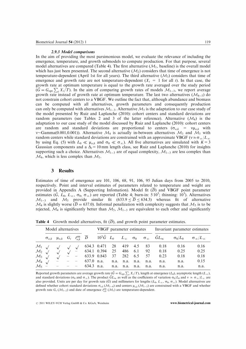
2.9.3 Model comparisonsIn the aim of providing the most parsimonious model, we evaluate the relevance of including theemergence, temperature, and growth submodels to compute production. For that purpose, severalmodel alternatives are compared (Table 4). The first alternative (M1, baseline) is the overall modelwhich has just been presented. The second alternative (M2) considers that time of emergence is nottemperature-dependent (April 1st for all years). The third alternative (M3) considers that time ofemergence and growth rate are not temperature-dependent (Xt 5 1 for all t). In that case, thegrowth rate at optimum temperature is equal to the growth rate averaged over the study period( �G ¼ Gopt

Pt Xt=T). In the aim of comparing growth rates of models M1�3, we report average

growth rate instead of growth rate at optimum temperature. The last two alternatives (M4�5) donot constrain cohort centers to a VBGF. We outline the fact that, although abundance and biomasscan be computed with all alternatives, growth parameters and consequently productioncan only be computed with alternativesM1�3. AlternativeM5 is the adaptation to our case study ofthe model presented by Ruiz and Laplanche (2010): cohort centers and standard deviations arerandom parameters (see Tables 2 and 3 of the latter reference). Alternative (M4) is theadaptation to our case study of the model discussed by Ruiz and Laplanche (2010): cohort centersare random and standard deviations are proportional to centers (so,k 5 nmo,k withn�Gamma(0.001,0.001)). Alternative M4 is actually in-between alternatives M3 and M5 withrandom centers while standard deviations are constrained with an approximate VBGF (nCsN/LN

by using Eq. (5) with L0 � mo,k and s0 � sN). All five alternatives are simulated with K5 3Gaussian components and a Dl 5 10mm length class, see Ruiz and Laplanche (2010) for insightssupporting such a choice. AlternativesM1�3 are of equal complexity,M1�3 are less complex thanM4, which is less complex thanM5.

3 Results

Estimates of time of emergence are 101, 106, 68, 91, 106, 95 Julian days from 2005 to 2010,respectively. Point and interval estimates of parameters related to temperature and weight areprovided in Appendix A (Supporting Infomation). Model fit (D) and VBGF point parameterestimates ( �G, L0, LN, s0, sN) are reported (Table 4; burn-in: 5 105; thinning: 103). AlternativesM1�3 and M5 provide similar fit (633:9 � D � 634:3) whereas fit of alternativeM4 is slightly worse (D ¼ 637:0). Informal penalization with complexity suggests thatM5 is to berejected, M4 is significantly better than M5, M1�3 are equivalent to each other and significantly

Table 4 Growth model alternatives, fit (D), and growth point parameter estimates.

Model alternatives VBGF parameter estimates Invariant parameter estimates

so,k mo,k Gt temo;k D 103 �G L0 LN s0 sN�GL1 s0/L0 sN/LN

M1p p p p 634.3 0.471 28 419 4.5 83 0.18 0.16 0.16

M2p p p – 634.1 0.394 25 486 6.1 92 0.18 0.25 0.25

M3p p – – 633.9 0.843 37 282 6.5 57 0.23 0.18 0.18

M4p – – – 637.0 n.a. n.a. n.a. n.a. n.a. n.a. n.a. 0.15

M5 – – – – 634.3 n.a. n.a. n.a. n.a. n.a. n.a. n.a. n.a.

Reported growth parameters are average growth rate ( �G ¼ Gopt

Pt Xt=T), length at emergence (L0), asymptotic length (LN),

and standard deviations (s0 and sN). The product �GL1 as well as the coefficients of variation s0/L0 and n C sN/LN are

also provided. Units are per day for growth rate (G) and millimeters for lengths (L0, LN, s0, sN). Model alternatives are

defined whether cohort standard deviations so;k (M1�4) and centers mo;k (M1�3) are constrained with a VBGF and whether

growth rate Gt (M1�2) and date of emergence temo;k (M1) are temperature-dependent.



better than M4. In other words, constraining cohort centers and/or standard deviationswith a VBGF does not (or slightly) worsen model fit while it significantly decreases complexity.As a result, alternatives M1�3 constraining both cohort centers mo,k and standard deviations so,k

with a VBGF are to be preferred. The improvement which is provided by modeling temperature-dependent time of emergence and growth rate is not significant, in favor of selectingalternative M3 for this case study. Nevertheless, in the aim of illustrating the modeling of tem-perature-dependent time of emergence and growth rate, following results are computed by usingbaseline (M1).

Raw VBGF point parameter estimates are variable across models. For that reason, we alsoprovide estimates of the product �GL1 as well as the coefficients of variation s0/L0 and sN/LN

(Table 4). We provide interval estimates of growth parameters by using alternative M1 (Table 5,Supporting Infomation). Interval estimates of �GL1 and sN/LN are of lesser amplitude thaninterval estimates of �G, LN, and sN, in favor of reporting the former parameter estimates instead ofraw VBGF parameters. This issue is discussed later.

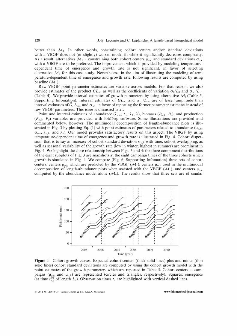
Point and interval estimates of abundance (lo,k, lo, lk, l), biomass (Bo,k, Bo), and production(Po,k, Po) variables are provided with HMSPop software. Some illustrations are provided andcommented below, however. The multimodal decomposition of length-abundance plots is illu-strated in Fig. 3 by plotting Eq. (1) with point estimates of parameters related to abundance (mo,k,so,k, to,k, and lo). Our model provides satisfactory results on this aspect. The VBGF by usingtemperature-dependent time of emergence and growth rate is illustrated in Fig. 4. Cohort disper-sion, that is to say an increase of cohort standard deviation so,k with time, cohort overlapping, aswell as seasonal variability of the growth rate (low in winter, highest in summer) are prominent inFig. 4. We highlight the close relationship between Figs. 3 and 4: the three-component distributionsof the eight subplots of Fig. 3 are snapshots at the eight campaign times of the three cohorts whichgrowth is simulated in Fig. 4. We compare (Fig. 6, Supporting Infomation) three sets of cohortcenters: centers �mo;k which are predicted by the VBGF (M1), centers mo,k used in the multimodaldecomposition of length-abundance plots when assisted with the VBGF (M1), and centers mo,kcomputed by the abundance model alone (M4). The results show that three sets are of similar

0

50

100

150

200

250

Time (year)

Fish

leng

th (

mm

)

2005 2006 2007 2008 2009 2010

Figure 4 Cohort growth curves. Expected cohort centers (thick solid lines) plus and minus (thinsolid lines) cohort standard deviations are computed by using the cohort growth model with thepoint estimates of the growth parameters which are reported in Table 5. Cohort centers at cam-paigns ð �mo;k and mo,k) are represented (circles and triangles, respectively). Squares: emergence(at time temo;k of length Lo). Observation times to are highlighted with vertical dashed lines.



values. Estimates of production over biomass ratios ((P/B)o,k and (P/B)o) are illustrated (Fig. 7,Supporting Infomation). (P/B)o values range between 1.03 and 1.59 per year.

4 Discussion

The results show that constraining cohort centers and standard deviations with a growth model is afruitful approach in the aim of interpreting length-abundance plots. As a corollary, the modeling ofindividual fish growth with a VBGF as well as the statistical model of Appendix B (SupportingInfomation) are decisive steps toward a refined interpretation of length-abundance plots. Ourfeeling is that advanced modeling has the potential to enhance the value of removal sampling databy leading to estimates of parameters with ecological meaning (e.g. growth rate). HBMs haveproven an efficient tool to fulfill this objective. Some choices have been made while constructing andsimulating our HBM, which are discussed below. We also suggest some possible refinements andextensions to the current HBM.

Model selection has shown that the improvement brought by modeling temperature-dependenttime of emergence and growth rate is not significant in this case study. The reasons are (i) stability oftemperature across years resulting in stability of time of emergence temo;k and averaged growth rate�Go;k and (ii) sampling occurring mostly around the same date resulting in stability of the length ofthe time period between emergence and campaign ðto � temo;kÞ, consequently resulting in stability ofthe cumulative growth rate �Go;kðto � temo;kÞ. The consideration of removal sampling campaigns morescattered across the year, or of a study area with more variable temperatures, or of a longer studyperiod, for instance in the aim of investigating the consequences of climate change on brown troutgrowth and production, would require the inclusion of temperature-dependent time of emergenceand growth rate.

HBM framework would make it technically possible to handle missing water temperature data,simulate raw water temperatures (ywt ) for the whole duration of the study, and use such tempera-tures to compute temperature-dependent growth parameters. We, however, chose to computetemperature-dependent parameters by using predictions of water temperature ðE½ywt �Þ instead of rawvalues ðywt Þ. We provide three reasons supporting this choice. First, the use of predictions of watertemperature instead of raw measurements leads to negligible consequences on computed time ofemergence and growth rate, as discussed later. Second, the computations of time of emergence andgrowth rate (sums in Eqs. 3 and 7) during the MCMC simulation are time-consuming. The lattersums can be precomputed by using predictions of water temperature instead of raw values. Third,our aim is to provide a layout to compute growth parameter estimates of brown trout populationsthat could apply to previously acquired removal sampling data. The motivation for that is toinvestigate consequences of climate change, for instance over the last decades. Air temperature isavailable posterior to electrofishing campaigns by simply making a query to meteorological data-bases. Water temperature is more difficult to acquire and, in our case study, such measurements areonly used to calibrate the air–water temperature submodel.

The joint simulation of the overall model was not feasible with the computation resources athand. For that reason, we have simulated the overall model into three steps. The sequence ofcomputations which is described below is illustrated in Fig. 1. The first step was to estimate theparameters of the weight and temperature submodels. Point parameter estimates of the lattersubmodels are used to predict fish weight (from fish length) and water temperature (from airtemperature). At the second step, predictions of water temperature are used to compute time ofemergence and growth rate. At the third step, the remaining submodels (abundance, growth, bio-mass, production) are simulated as a full HBM. We outline the fact that precomputation isolatessubmodels from the consecutive fully Bayesian inference. We see two consequences of that. First,presimulated submodels (e.g. emergence) cannot borrow information from other submodels(e.g. growth) to provide an improved estimation of parameters (e.g. CE50). An extended discussion



on this issue is provided later. Second, uncertainty of parameters of precomputed submodels (e.g.Zo) is not propagated to parent submodels (e.g. biomass). Potential consequences would be anunderestimation of the variance of the estimate of parameters of interest (e.g. Bo,k). A solution tothe latter issue could be not to convey input values as fixed (as we have done here) but rather asrandom. In our case, however, the consequences of using fixed input values are negligible. Thereason for that is that fish weights are summed to compute biomass, functions of water temperatureare summed to compute time of emergence (Eq. 7) and growth rate (Eq. 3). See Ruiz and Laplanche(2010) for a demonstration regarding the consequences of using predictions of fish weight (insteadof raw values with residual error) to compute biomass.

Estimates of growth parameters �G, LN, and sN are highly uncertain (Table 5, SupportingInfomation). The reason for that is that sports fishing takes place in the Neste d’Oueil from Marchto September with a 180mm minimum size limit. Large, and consequently old, brown trouts arerare. The VBGF is approximately linear of slope �GL1 for young fish, it is not feasible to jointlyprovide accurate estimates of �G and LN by using our data set. It is not either feasible to jointlyprovide accurate estimates of LN and sN (Eq. 5 approximates to so;k ’ ðs1=L1Þmo;k as shownearlier). We suggest three options. The first option, which we have chosen here, is to report morerobust parameters such as �GL1 and sN/LN. The product �GL1 is a life-history invariant which hasalready been reported in the literature (Mangel, 1996; Hutchings, 2002). The second option wouldbe to provide multimodel estimates (Burnham and Anderson, 2002). The third option would be touse a distinct data set, e.g. collected in a fishing preserve, to provide estimates of �G, LN, and sN.Estimation of length at emergence L0 is relatively less uncertain. L0 estimate is contingent onprecalculated time of emergence, which is a function of temperature and time of oviposition. Timeof emergence actually depends on more covariates, e.g. discharge (Capra et al., 2003). Time ofoviposition has been roughly (in the absence of more appreciable information) assumed equal for allyears. Oviposition timing is not punctual and depends on covariates. As a result, our estimatesof L0 should be considered with caution. An over (under) estimation of oviposition timing leads toan over (under) estimation of L0. An inaccurate estimation of oviposition timing has, however,negligible consequences on other parameters (since L0 is adjusted accordingly). Estimation of s0,and as a result s0/L0, are uncertain. The posterior distribution of s0 (or quantiles, Table 5, Sup-porting Infomation) suggests to reduce of our growth model with s0 5 0. As a conclusion, wesuggest to give credential to parameters �GL1 and sN/LN and consider remaining parameters withcaution.

HBM framework would make it technically possible to handle cardinal temperatures (ymin, ymax,yopt, y0, y1) as well as date of oviposition and critical value EC50 as random. The motivation for thatwould be to propagate the uncertainty of our knowledge on such parameters to estimates ofremaining parameters. We have nevertheless considered cardinal temperatures, date of oviposition,and EC50 as constant. The main reason is that removal sampling data does not contains enoughinformation to enhance our knowledge on the above parameters plus L0 and Gopt. Randomizingcardinal temperatures, date of oviposition, and EC50 would result in randomizing time of emergenceand cardinal growth rate. It is not possible, however, due to under-identification, to providerelevant estimates of time of emergence together with length at emergence (both represent varia-bility of emergence) neither provide relevant estimates of cardinal growth rate together with opti-mum growth rate (both represent variability of growth rate). We chose to set constant time ofemergence and cardinal growth rate (by setting constant cardinal temperatures, date of oviposition,and EC50) in order to provide estimates of L0 and Gopt. The interest of setting constant the formerparameters is also to be able to carry out the (necessary) precomputations of time of emergence andcardinal growth rate.

Residuals �mo;k � mo;k are low (sm 5 0.7 (0.5, 1.3) mm) but are not negligible (Fig. 4). Residualswould be negligible if the reduction of the current model with the constraint of null residualsprovided satisfactory results. Such a reduction did not provide satisfactory results (not shown) andwe suggest several possible countermeasures. We have linearly interpolated monthly and 10-day air



temperatures to a daily time step. The use of daily air temperature measurements would be a firstimprovement. A more complex modeling of stream temperature, e.g. as a function of minimum andmaximum daily air temperature and stream discharge, is a second option. A more complex mod-eling of the growth rate, e.g. as a function of discharge (Daufresne and Ranault, 2006), is a thirdoption. The use of a more advanced statistical model of growth parameters, e.g. by correlatinggrowth rate to asymptotic length or by adding an autoregressive component to the growth rate, is apossibility. At last, the use of a different growth function is also conceivable.

The model at the current state applies to riverine brown trout (S. trutta fario). Main modelassumptions are that (i) reproduction occurs once a year, (ii) growth and emergence are pre-dominantly dependent on water temperature, and (iii) temperature history at the stream section is arelevant indicator of temperature to which captured fish have been subjected to. Additionaldevelopments would be required to apply the model to species with a migrating behavior (e.g.brown trout morphs S. trutta trutta and lacustris) or with a different reproduction pattern. S. truttafario also migrates, but operates low amplitude movements in order to switch for microhabitats. Wehighlight the fact that, for not to disturbing such natural movements as well as for practical reasons,we did not physically delimited the stream section across campaigns. Microhabitat movements areof limited consequences on temperature to which fish are subjected to. Temporal variations ofabundance, however, are to be interpreted with caution: abundance (lo) is not synonymous withpopulation size. Abundance is not representative of the size of a closed brown trout populationinhabiting a stream section (such a population is fictional). Abundance rather depicts the status of asingle species at a single place, which temporal variations are the result of some complex populationdynamics. Finally, the stream section is not either physically delimited across removals. Results arepotential entries and exits of fish during electrofishing, e.g. downstream exits of stunned but notcaught fish. Consequences of the latter movements are an overestimate of electrofishing efficiencyand an underestimate of abundance. A solution to this issue would be to position nets down- andup-stream while electrofishing.

To conclude, we highlight some possible extensions to the current model. First, the growth modelcould be perfected, as suggested above. Date of oviposition could be modeled and related tocovariates. Removal sampling data could be accompanied with age data in the aim offacilitating cohort decomposition. To achieve this goal, age of fish could be evaluated throughscalimetry (age is determined by counting growth zones of fish scales magnified with a microscope)on a sample of caught fish and treated as missing data on the rest. The model could beextended with an additional spatial structure in order to deal with multiple sampling sections(Wyatt, 2002; Ebersole et al., 2009; Ruiz and Laplanche, 2010). Parameters (e.g. growth parameters)could be spatially related to each other or related to spatially distributed environmental covariates(Wyatt, 2003; Webster et al., 2008). Parameters of the multimodal description of length-abundanceplots are cohort centers, standard deviations, and weights (to,k) as well as total abundance (lo). Wehave constrained centers and standard deviations with a growth model. Weights and abundancecould also be constrained with a population dynamics submodel. Parameters of the populationdynamics submodel could be spatially related to each other or to covariates. The motivation is tobuild a single framework which would provide interval estimates of a large panel of descriptorsindicative of brown trout populations at a large spatio-temporal scale. Such a model could be usedto evaluate, compare, and predict the status of brown trout populations, e.g. consequently toclimate change.

Acknowledgements The authors are indebted to L. Pacaux, F. Dauba, and P. Lim (Ecolab) for their con-tribution in conducting the electrofishing campaign and collecting the removal sampling data set. The authorsare grateful to EDF R&D for financing the electrofishing campaign and providing the water temperature dataset. The authors thank both anonymous referees for their valuable, detailed reviews which significantly im-proved the clarity of the manuscript. This work was granted access to the HPC resources of CALMIP underthe allocation 2011-P1113



Conflict of interest

The authors have declared no conflict of interest.

References

Armstrong, J., Kemp, P., Kennedy, G., Ladle, M. and Milner, N. (2003). Habitat requirements of atlanticsalmon and brown trout in rivers and streams. Fisheries Research 62, 143–170.

Bertalanffy, L. (1938). A quantitative theory of organic growth (inquiries on growth laws II). Human Biology10, 181–213.

Burnham, K. and Anderson, D. (2002). Model Selection and Multimodel Inference: A Practical Information-Theoretic Approach. 2nd edn., Springer, Berlin.

Caissie, D. (2006). The thermal regime of rivers: a review. Freshwater Biology 51, 1389–1406.Capra, H., Sabaton, C., Gouraud, V., Souchon, Y. and Lim, P. (2003). A population dynamics model and

habitat simulation as a tool to predict brown trout demography in natural and bypassed stream reaches.River Research and Applications 19, 551–568.

Carle, F. and Strub, M. (1978). A new method for estimating population size from removal data. Biometrics 34,621–630.

Chen, Y., Jackson, D. and Harvey, H. (1992). A comparison of von Bertalanffy and polynomialfunctions in modelling fish growth data. Canadian Journal of Fisheries and Aquatic Sciences 49,1128–1235.

Congdon, P. (2006). Bayesian Statistical Modelling. Wiley Series in Probability and Statistics. 2nd edn.Wiley,Chichester, England.

Crawley, M. (2007). The R Book. Wiley, New York.Daufresne, M. and Renault, O. (2006). Population fluctuations, regulation and limitation in stream-living

brown trout. Oikos 113, 459–468.Dorazio, R., Jelks, H. and Jordan, F. (2005). Improving removal-based estimates of abundance by sampling a

population of spatially distinct subpopulations. Biometrics 61, 1093–1101.Ebersole, J., Colvin, M., Wigington, P., Leibowitz, S., Baker, J., Church, M., Compton, J. and Cairns, M.

(2009). Hierarchical modeling of late-summer weight and summer abundance of juvenile Coho Salmonacross a stream network. Transactions of the American Fisheries Society 138, 1138–1156.

Elliott, J. (1994). Quantitative Ecology and the Brown Trout. Oxford University Press, Oxford, UK.Elliott, J. and Hurley, M. (1998). An individual-based model for predicting the emergence period of sea trout

fry in a lake district stream. Journal of Fish Biology 53, 414–433.Elliott, J., Hurley, M. and Fryer, R. (1995). A new, improved growth model for brown trout, Salmo trutta.

Functional Ecology 9, 290–298.Fontoura, N. and Agostinho, A. (1996). Growth with seasonally varying temperatures – an expansion of the

von Bertalanffy growth model. Journal of Fish Biology 48, 569–584.Froese, R. and Pauly, D. (2010). Fishbase. World Wide Web electronic publication. www.fishbase.orgGelman, A., Carlin, J., Stern, H. and Rubin, D. (2003). Bayesian Data Analysis. Chapman & Hall/CRC, Boca

Raton, Florida.Gelman, A. and Rubin, D. (1992). Inference from iterative simulation using multiple sequences. Statistical

Science 7, 457–472.Gouraud, V., Bagliniere, J., Baran, P., Sabaton, C., Lim, P. and Ombredane, D. (2001). Factors regulating

brown trout populations in two french rivers: application of a dynamic population model. RegulatedRivers: Research & Management 17, 557–569.

Hutchings, J. (2002). Life histories of fish. In: Handbook of Fish Biology and Fisheries. Vol. 1, Blackwell ScienceLtd, Malden, USA, pp. 149–174.

Jensen, A. and Johnsen, B. (1999). The functional relationship between peak spring floods and survival andgrowth of juvenile Atlantic salmon (Salmo salar) and brown trout (Salmo trutta). Functional Ecology 13,778–785.

Jonsson, B. and Jonsson, N. (2009). A review of the likely effects of climate change on anadromous atlanticsalmon Salmo salar and brown trout Salmo trutta, with particular reference to water temperature and flow.Journal of Fisheries Biology, 75, 2381–2447.



Klemetsen, A., Amundsen, P.-A., Dempson, J., Jonsson, B., Jonsson, N., OConnell, M. and Mortensen, E.(2003). Atlantic salmon Salmo salar l., brown trout Salmo trutta l. and arctic charr Salvelinus alpinus (l.): areview of aspects of their life histories. Ecology of Freshwater Fish 12, 1–59.

Kwak, J. and Waters, T. (1997). Trout production dynamics and water quality in Minnesota streams.Transactions of the American Fisheries Society 126, 35–48.

Lagadic, L., Caquet, T., Amiard, J.-C. and Ramade, F. (1998). Utilisation de biomarqueurs pour la surveillancede la qualite de l’environnement. Lavoisier TEC DOC, Paris.

Laplanche, C. (2010). A hierarchical model to estimate fish abundance in alpine streams by using removalsampling data from multiple locations. Biometrical Journal, 52, 209–221.

Lobon-Cervia, J. (1991). Dinamica de poblaciones de peces en rıos: pesca electrica y metodos de capturassucesivas en la estima de abundancias. Monografıas del Museo Nacional de Ciencias Naturales,Madrid.

Lunn, D., Spiegelhalter, D., Thomas, A. and Best, N. (2009). The BUGS project: Evolution, critique and futuredirections. Statistics in Medicine 28, 3049–3067.

Mallet, J., Charles, S., Persat, H. and Auger, P. (1999). Growth modelling in accordance with daily watertemperature in European grayling (Thymallus thymallus L.). Canadian Journal of Fisheries and AquaticSciences 56, 994–1000.

Mangel, M. (1996). Life history invariants, age at maturity and the ferox trout. Evolutionary Ecology, 10,249–263.

Mantyniemi, S., Romakkaniemi, A. and Arjas, E. (2005). Bayesian removal estimation of a population sizeunder unequal catchability. Canadian Journal of Fisheries and Aquatic Sciences 62, 291–300.

Mohseni, O., Stefan, H. and Erickson, T. (1998). A nonlinear regression model for weekly stream temperatures.Water Resource Research 34, 2685–2692.

Morrill, J., Bales, R. and Conklin, M. (2005). Estimating stream temperature from air temperature: implica-tions for future water quality. Journal of Environmental Engineering 131, 139–146.

Nash, J. and Sutcliffe, J. (1970). River flow forecasting through conceptional models, 1. a discussion ofprinciples. Journal of Hydrology 10, 282–290.

Nordwall, F., Naslund, I. and Degerman, E. (2001). Intercohort competition effects on survival, movement,and growth of brown trout (Salmo trutta) in Swedish streams. Canadian Journal of Fisheries and AquaticSciences 58, 2298–2308.

Ntzoufras, I. (2009). Bayesian Modeling Using WinBUGS. Wiley, Hoboken, NJ.Pauly, D. and Moreau, J. (1997). Methodes pour l’evaluation des ressources halieutiques. Cepadues-Editions,

Toulouse, France.Peterson, J., Thurow, R. and Guzevich, J. (2004). An evaluation of multipass electrofishing for estimating

the abundance of stream-dwelling salmonids. Transactions of the American Fisheries Society 133,462–475.

Pinheiro, J. and Bates, D. (2000). Mixed-Effects Models in S and S-Plus. Springer, Berlin.Pitcher, T. (2002). A bumpy old road: Sized-based methods in fisheries assessment. In: Handbook of Fish

Biology and Fisheries, Vol. 2, Blackwell Science Ltd., Malden, USA, pp. 189–210.Polard, T., Jean, S., Gauthier, L., Laplanche, C., Merlina, G., Sanchez-Perez, J.-M. and Pinelli, E. (2011).

Mutagenic impact on fish of runoff events in agricultural areas in south-west france. Aquatic Toxicology101, 126–134.

Quinn, T. and Deriso, R. (1999). Quantitative Fish Dynamics. Oxford University Press, USA.Riley, S. and Fausch, K. (1992). Underestimation of trout population size by maximum likelihood

removal estimates in small streams. North American Journal of Fisheries Management 12,768–776.

Rivot, E., Prevost, E., Cuzol, A., Bagliniere, J.-L. and Parent, E. (2008). Hierarchical Bayesian modelling withhabitat and time covariates for estimating riverine fish population size by successive removal method.Canadian Journal of Fisheries and Aquatic Science 65, 117–133.

Robert, C. and Casella, G. (2004). Monte Carlo Statistical Methods. 2nd edn., Springer, New York.Rosso, L., Lobry, J., Bajard, S. and Flandrois, J. (1995). Convenient model to describe the combined effects of

temperature and ph on microbial growth. American Society for Microbiology 61, 610.Ruiz, P. and Laplanche, C. (2010). A hierarchical model to estimate the abundance and biomass of salmonids

by using removal sampling and biometric data from multiple locations. Canadian Journal of Fisheries andAquatic Science 67, 2032–2044.



Shinn, C. (2010). Impact of toxicants on stream fish biological traits. PhD thesis, Universite de Toulouse.Somers, I. (1988). On a seasonally-oscillating growth function. Fishbyte 6, 8–11.Spiegelhalter, D., Best, N., Carlin, B. and van der Linde, A. (2002). Bayesian measures of model complexity

and fit. Journal of the Royal Statistical Society Series B 64, 583–639.Taylor, C. (1960). Temperature, growth, and mortality – the pacific cockle. ICES Journal of Marine Science 26,

117.Ward, R. (2002). Genetics of fish populations. In: Handbook of Fish Biology and Fisheries, vol. 1, Blackwell

Science Ltd., Malden, USA, pp. 200–224.Webb, J. and McLay, H. (1996). Variation in the time of spawning of Atlantic salmon (Salmo salar) and its

relationship to temperature in the Aberdeenshire Dee, Scotland. Canadian Journal of Fisheries and AquaticScience 53, 2739–2744.

Webster, R. A., Pollock, K. H., Ghosh, S. K. and Hankin, D. G. (2008). Bayesian spatial modelingof data from unit-count surveys of fish in streams. Transactions of the American Fisheries Society 137,438–453.

Wood, C. (2007). Global warming: implications for freshwater & marine fish. In: Society for ExperimentalBiology Seminar Series, Vol. 61, Cambridge University Press, Cambridge.

Wyatt, R. (2002). Estimating riverine fish population size from single- and multiple-pass removal samplingusing a hierarchical model. Canadian Journal of Fisheries and Aquatic Science 59, 695–706.

Wyatt, R. (2003). Mapping the abundance of riverine fish populations: integrating hierarchical Bayesianmodels with a geographic information system (GIS). Canadian Journal of Fisheries and Aquatic Science 60,997–1006.



Documents

A length-based hierarchical model of brown trout (Salmo trutta fario) growth and production