Embed Size (px)
Citation preview
INTERNATIONAL JOURNAL FOR NUMERICAL METHODS IN ENGINEERINGInt. J. Numer. Meth. Engng 2011; 86:358–380Published online 17 December 2010 in Wiley Online Library (wileyonlinelibrary.com). DOI: 10.1002/nme.3069
A level set based model for damage growth: The thick level setapproach
N. Moës1,∗,†, C. Stolz2, P.-E. Bernard1 and N. Chevaugeon1
1GeM Institute, École Centrale de Nantes/Université de Nantes/CNRS 1 Rue de la Noë, 44321 Nantes, France2Laboratoire de Mécanique des Solides, CNRS UMR 7649, École Polytechnique, 91128 Palaiseau, France
SUMMARY
In this paper, we introduce a new way to model damage growth in solids. A level set is used to separatethe undamaged zone from the damaged zone. In the damaged zone, the damage variable is an explicitfunction of the level set. This function is a parameter of the model. Beyond a critical length, we assume thematerial to be totally damaged, thus allowing a straightforward transition to fracture. The damage growthis expressed as a level set propagation. The configurational force driving the damage front is non-localin the sense that it averages information over the thickness in the wake of the front. The computationaland theoretical advantages of the new damage model are stressed. Numerical examples demonstrate thecapability of the new model to initiate cracks and propagate them even in complex topological patterns(branching and merging for instance). Copyright � 2010 John Wiley & Sons, Ltd.
Received 19 January 2010; Revised 8 September 2010; Accepted 21 September 2010
KEY WORDS: level set; damage; X-FEM; fracture
1. INTRODUCTION
It is well known that fracture mechanics alone may not model the full scenario of the degradationof solids under mechanical loading. Crack initiation for instance requires damage mechanics tomodel the gradual loss of stiffness in a small area [1, 2]. When it comes to modelling damage,special care needs to be taken to avoid so-called spurious localizations. Several damage modelswere proposed in the literature to avoid spurious localization as detailed in [3, 4]:
• non-local integral damage model: the damage evolution is governed by a driving force whichis non-local, i.e. it is the average of the local driving force over some regions [5, 6];
• higher order, kinematically based, gradient models through the inclusion of higher orderdeformation gradient [7–9] or additional rotational degrees of freedom [10];
• higher order, damage based, gradient models: the gradient of the damage is a variable as wellas the damage itself. This leads to a second-order operator acting on the damage [11–13].
Non-local and higher order gradient approaches were compared in [14]. More recently twostrategies to avoid spurious localization also appeared. The phase-field approach emanating fromthe physics community [15–17] and the so-called variational approach [18–20].
In this paper, we wish to model damage as a propagating level set front. Let us first tour theexisting papers using a level set approach to model a degradation front. In report [21] a level
∗Correspondence to: N. Moës, GeM Institute, École Centrale de Nantes, Université de Nantes, CNRS, 1 Rue de laNoë, 44321 Nantes, France.
†E-mail: [email protected]
Copyright � 2010 John Wiley & Sons, Ltd.
LEVEL SET BASED MODEL FOR DAMAGE GROWTH 359
set is introduced to separate a totally damaged zone from an undamaged zone. The growth ofthe level is governed by a criterion: the front advances if the corresponding configurational force(called shape gradient by the authors) reaches a critical value, say Yc. When no front is initiallypresent, the authors suggest to use the topological derivative as the driving force and compare itwith the critical value. We note that the model of [21] does not introduce a length and will mostlikely suffer pathological mesh-dependencies known in the computational mechanics communityas spurious localization. This model will also most likely be unable to model a size-effect.
In the same spirit the evolution of the interface � separating sound material from damagedmaterial has been studied in [22, 23] using an energetical description for the propagation. Thedriving force associated with the normal velocity of the front is a local release rate of energy. Usingnormality rule to govern the propagation, the rate boundary value problem in terms of displacementand motion of the interface is studied and conditions of existence and uniqueness are given.
In paper [24], Moës et al. use basically the same model as in [21], but with an importantdifference that a surface energy term is added. This added energy term was introduced by Nguyenet al. [25]. It is shown that this added energy contributes to stabilize the system so that no bifurcationis observed during the interface propagation. The configurational force on the interface must nowreach the critical value Yc +�c/� in which � is the radius of curvature of the interface and �c acritical surface energy. This avoids the creation of spikes on the interface since � will becomevery small and the criterion to meet very high. As a by-product, the model introduces the lengthscale lc =�c/Yc. The meaning of the length is however not clear at this time. The drawback ofthis curvature regularized model is that the energy to initiate a small hole is infinite since �=0+at void initiation. Without this critical surface energy nucleation of defects can also be consideredas a bifurcation of equilibrium solution [26].
Somehow, one would like to use the criterion of [21] based on the topological derivativecompared with Yc to nucleate a void and then use the model [25] to evolve the void withoutspurious localizations. When should the switch take place is not a trivial question. Finally, in thematerial science community, note that paper [27] also introduces a level set technique to distinguishvoids from matter. The growth criterion in the above paper is simply �c/�. The authors modelnano crack patterns. Nothing is said in this paper regarding nucleation.
In [21, 27], the authors do not consider the damaged region to be totally damaged but do leavesome stiffness in it. On the contrary, in [24] the front is modeled by the extended finite elementmethod (X-FEM) allowing the damaged zone to be truly of zero stiffness. This avoids non-physicaldegradation behind the crack tip since the crack may now open freely. Still, from the numericalstand point, Moës et al. [24] introduced a proper method to evaluate the loading (indeed as damageprogresses the load must usually decrease and snap-back may occur).
After this description of level set based damage front model, let us turn to the phase-fieldapproach developed for fracture in the physics community [15–17]. On the contrary to the levelbased approach, there is no longer with the phase-field approach a strict boundary between onematerial phase (damaged) and the other one (fully damaged). A transition zone is present.
In the phase-field approach a parameter �, called phase, is introduced to describe the transitionand varies from 0 (no damage) to 1 (total damage). A global phase equation coupled to themechanical equations is solved in order to determine the phase value at each point in the domain.The phase-field equation involves a Laplacian of the phase that introduces a length scale and mostlikely kills spurious localization of the phase. This resolution is made over the whole domain. Thedamage is a given function of the phase field.
The goal of this paper is to introduce a new regularization for local damage models. The mainidea is to keep the simplicity of the level set through a propagation algorithm while keeping inits wake a transition zone in which the material degrades over a given length. The advantage ofdealing with damage represented by a level set is that it is well known that a level set propagationmay be solved close only to the level set front.
Within the transition zone, damage is an explicit function of the level set. This function is aparameter of the model. Beyond a critical distance to the level set front the damage is assumed tobe 1. In other words, as the front propagates it unveils in its wake a fully damaged zone. We call
Copyright � 2010 John Wiley & Sons, Ltd. Int. J. Numer. Meth. Engng 2011; 86:358–380DOI: 10.1002/nme
360 N. MOËS ET AL.
this zone the crack (although we shall see it is not necessarily of zero thickness). This zone maybe of very complex topology, thus dealing easily with branching and merging. In our approach, wethus do not need a transition to a cohesive crack to handle full degradation as in [28–30]. The crackappears as a consequence of the damage front motion. Finally, note that in the presented approach,the fully damaged zone is clearly delimited by a level set. It is thus not a set of elements similarto the element deletion approach [31]. Moreover, this zone is still allowed to carry compressiveloading if needed.
2. A NEW LEVEL SET BASED DAMAGE MODEL
It is well known that purely local damage models suffer from spurious localization because nolength scale is introduced in the models. In this paper, we introduce a length lc in the wake ofthe front creating what we call a thick level set (TLS). The damage depends on a signed distancefunction to the front. This description induces a specific evolution law for the damage, the evolutionfollows the motion of the level set. The damage itself could be regarded as a level set, but topreserve the generality of the approach, we choose to separate the evolution of the geometrydescribed by the level set and the associated value of damage.
In order to introduce the TLS approach we consider a simple damage model: an elasto-damagemodel with a scalar damage parameter.
2.1. A simple local damage model
The free energy per unit volume � depends on the strain ε and a scalar damage variable denotedby d
�=�(ε,d) (1)
The state laws are obtained by differentiating the free energy
r= ��
�ε, Y =−��
�d(2)
where r is the stress and Y the local energy release rate. For instance, if we consider a symmetricbehavior in traction and compression, we may use the potential
�(ε,d)= 12 (1−d) ε :E :ε (3)
leading to
r= (1−d) E :ε, Y = 12ε :E :ε (4)
A potential with closure effect will also be considered later in the numerical simulations. Theevolution of the damage is given by a dissipation potential �∗(Y ) which is a convex function of Y :
d = ��∗(Y )
�Y(5)
Alternatively, we may write
Y = ��(d)
�d(6)
The above potentials �(d) and �∗(Y ) are dual and related by the Legendre–Fenchel transformation
�(d)=supY
(Y d −�∗(Y )), �∗(Y )=supd
(Y d −�(d)) (7)
Copyright � 2010 John Wiley & Sons, Ltd. Int. J. Numer. Meth. Engng 2011; 86:358–380DOI: 10.1002/nme
LEVEL SET BASED MODEL FOR DAMAGE GROWTH 361
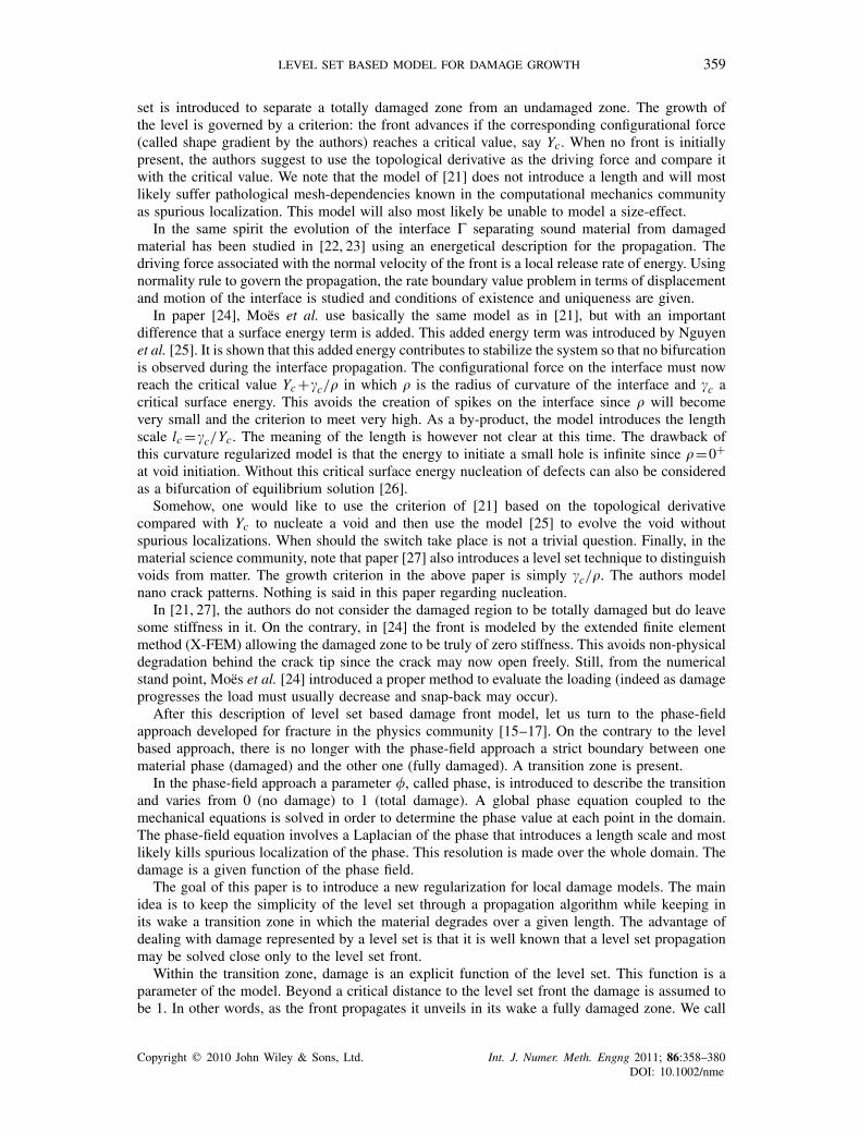
Figure 1. Multiple damaged, undamaged and transition zones are described using only one level set.
For non-regular functions, the definition of the gradient is replaced by the notion of sub-gradientY ∈��(d) if
�(d)+Y (d∗− d)��(d∗) (8)
for all admissible d∗. A similar definition is associated to �∗.Note that from the above we have the following inequality for any couple (Y, d) satisfying or
not the damage evolution law
�∗(Y )+�(d)−Y d�0 (9)
The equality is satisfied if and only if the damage evolution law is satisfied too:
�∗(Y )+�(d)−Y d =0⇔ d = ��∗(Y )
�Y⇔Y = ��(d)
�d(10)
Note that the convexity of � or �∗ ensure positive dissipation, this is due to (8) considering theproperties
�(d) convex, �(d)�0, �(0)=0 (11)
The damage model described above suffers from spurious localizations. To regularize this situation,we introduce a length scale in a different way than that proposed in the literature.
2.2. Free energy and state laws for the level set based damage model
The damage description is depicted in Figure 1. The level set �=0 separates the domain �into an undamaged zone and damaged one. In the damaged zone, the damage variable d is anexplicit function of the level set. Note that a single level set is needed even if damaged zones aredisconnected as shown in Figure 1.
The damage increases progressively as the level set value rises. Mathematically this is expressedby the following inequalities:
d(�) = 0, ��0 (12)
d ′(�) � 0, 0���lc (13)
d(�) = 1, ��lc (14)
Copyright � 2010 John Wiley & Sons, Ltd. Int. J. Numer. Meth. Engng 2011; 86:358–380DOI: 10.1002/nme
362 N. MOËS ET AL.
The function d =d(�) is assumed to be continuous for clarity. Discontinuous functions can bechosen in the proposed approach but the obtained expressions must be modified with additionalcontributions. At a distance lc from the damage front, the material is assumed completely damaged.A spatial relationship between the damage value along the normal to the front �=0 is then deduced.
Consider a body �. Along the external boundary ��, loading T d (t) is applied on ��T anddisplacements ud (t) are prescribed on the complementary part ��u ; ��=��T ∪��u , ��T ∩��u =∅. Some parts of � may be totally damaged i.e. d =1. We denote by �c, the part of � not fullydamaged:
�c ={x∈� :�(x)�lc} (15)
Potential energy is written as a function of the displacement field and the level set function �:
E(u,�)=∫
�c
�(ε(u),d(�))d�−∫
��T
T·u dS (16)
where ε(u) denotes the strain, i.e. symmetric part of the gradient of u. The displacement field mustsatisfy the kinematic boundary conditions whereas the gradient of the level set field must be ofnorm 1 since it is a signed distance function.
The function d(�) is assumed to be continuous. The displacement, the free energy and thestress vector are then continuous functions along each iso-� curve ��. Otherwise, a more complexexpression involving jump terms must be written. Along �� the displacement is continuous, then[u]��(x, t)=0 for x(t) on the moving surface ��(t). Then [u]�� + x.[∇u]�� =0, where x is thevelocity of ��. Any variation of displacement and variation of �� are linked by this equation ofcompatibility
[�u]�� +�vnn·[∇u]�� =0 (17)
But the continuity of d ensures the continuity of �. The stress vector and displacement gradientare thus also continuous. Then no jumps exist along the moving surfaces. Then the variations ofthe displacement and the variations of the moving surface �� are uncoupled.
The above conditions define the admissible set of variables Ad
Ad = {(u,�) :u∈ Aud , �∈ A�
d } (18)
Aud = {u :u defined on �c, u=u on ��u} (19)
A�d = {� :‖∇�‖=1 on �} (20)
The set of admissible variations is then defined by
A0 = {(�u,��) :�u∈ Au0, ��∈ A�
0 } (21)
Au0 = {�u :�u=0 on ��u} (22)
A�0 = {�� :∇��·∇�=0 on �} (23)
The condition on �� indicates that to remain a signed distance the level set variation must beconstant if we follow a path along the gradient of �. In order to visualize this property, let usconsider a plane situation as depicted in Figure 2 with the band of material comprised between theboundaries �0 and �c. This band may be parametrized by two curvilinear coordinates � and s,where s is the curvilinear abscissa along �0. The iso-coordinate curves are orthogonal to eachother. The condition (23) implies that �� is a function of s only and must be seen as a normalperturbation of the � front location. We may then write
��=�a(s) (24)
Copyright � 2010 John Wiley & Sons, Ltd. Int. J. Numer. Meth. Engng 2011; 86:358–380DOI: 10.1002/nme
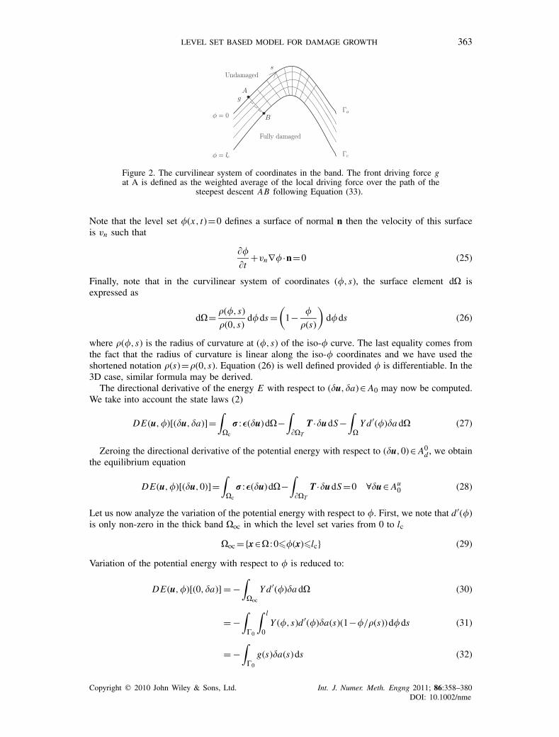
LEVEL SET BASED MODEL FOR DAMAGE GROWTH 363
Figure 2. The curvilinear system of coordinates in the band. The front driving force gat A is defined as the weighted average of the local driving force over the path of the
steepest descent AB following Equation (33).
Note that the level set �(x, t)=0 defines a surface of normal n then the velocity of this surfaceis vn such that
��
�t+vn∇�·n=0 (25)
Finally, note that in the curvilinear system of coordinates (�,s), the surface element d� isexpressed as
d�= �(�,s)
�(0,s)d�ds =
(1− �
�(s)
)d�ds (26)
where �(�,s) is the radius of curvature at (�,s) of the iso-� curve. The last equality comes fromthe fact that the radius of curvature is linear along the iso-� coordinates and we have used theshortened notation �(s)=�(0,s). Equation (26) is well defined provided � is differentiable. In the3D case, similar formula may be derived.
The directional derivative of the energy E with respect to (�u,�a)∈ A0 may now be computed.We take into account the state laws (2)
DE(u,�)[(�u,�a)]=∫
�c
r :ε(�u)d�−∫
��T
T·�udS−∫
�Y d ′(�)�a d� (27)
Zeroing the directional derivative of the potential energy with respect to (�u,0)∈ A0d , we obtain
the equilibrium equation
DE(u,�)[(�u,0)]=∫
�c
r :ε(�u)d�−∫
��T
T·�udS =0 ∀�u∈ Au0 (28)
Let us now analyze the variation of the potential energy with respect to �. First, we note that d ′(�)is only non-zero in the thick band �oc in which the level set varies from 0 to lc
�oc ={x∈� :0��(x)�lc} (29)
Variation of the potential energy with respect to � is reduced to:
DE(u,�)[(0,�a)] = −∫
�oc
Y d ′(�)�a d� (30)
= −∫
�0
∫ l
0Y (�,s)d ′(�)�a(s)(1−�/�(s))d�ds (31)
= −∫
�0
g(s)�a(s)ds (32)
Copyright � 2010 John Wiley & Sons, Ltd. Int. J. Numer. Meth. Engng 2011; 86:358–380DOI: 10.1002/nme
364 N. MOËS ET AL.
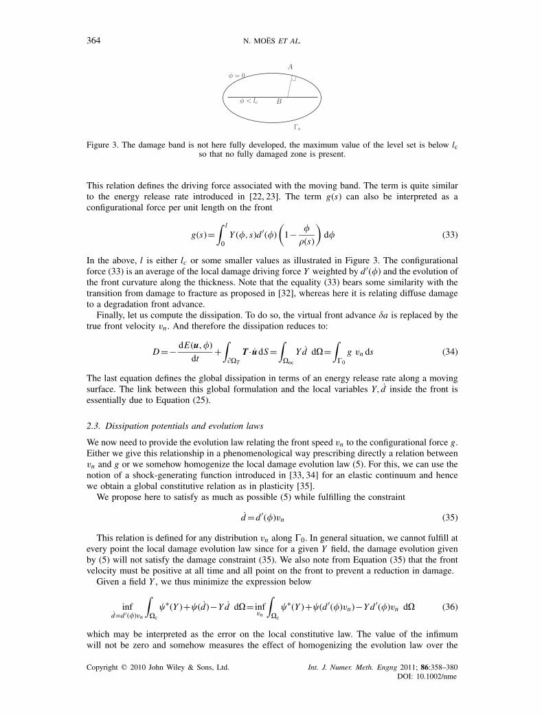
Figure 3. The damage band is not here fully developed, the maximum value of the level set is below lcso that no fully damaged zone is present.
This relation defines the driving force associated with the moving band. The term is quite similarto the energy release rate introduced in [22, 23]. The term g(s) can also be interpreted as aconfigurational force per unit length on the front
g(s)=∫ l
0Y (�,s)d ′(�)
(1− �
�(s)
)d� (33)
In the above, l is either lc or some smaller values as illustrated in Figure 3. The configurationalforce (33) is an average of the local damage driving force Y weighted by d ′(�) and the evolution ofthe front curvature along the thickness. Note that the equality (33) bears some similarity with thetransition from damage to fracture as proposed in [32], whereas here it is relating diffuse damageto a degradation front advance.
Finally, let us compute the dissipation. To do so, the virtual front advance �a is replaced by thetrue front velocity vn . And therefore the dissipation reduces to:
D =− dE(u,�)
dt+∫
��T
T·udS =∫
�oc
Y d d�=∫
�0
g vn ds (34)
The last equation defines the global dissipation in terms of an energy release rate along a movingsurface. The link between this global formulation and the local variables Y, d inside the front isessentially due to Equation (25).
2.3. Dissipation potentials and evolution laws
We now need to provide the evolution law relating the front speed vn to the configurational force g.Either we give this relationship in a phenomenological way prescribing directly a relation betweenvn and g or we somehow homogenize the local damage evolution law (5). For this, we can use thenotion of a shock-generating function introduced in [33, 34] for an elastic continuum and hencewe obtain a global constitutive relation as in plasticity [35].
We propose here to satisfy as much as possible (5) while fulfilling the constraint
d =d ′(�)vn (35)
This relation is defined for any distribution vn along �0. In general situation, we cannot fulfill atevery point the local damage evolution law since for a given Y field, the damage evolution givenby (5) will not satisfy the damage constraint (35). We also note from Equation (35) that the frontvelocity must be positive at all time and all point on the front to prevent a reduction in damage.
Given a field Y , we thus minimize the expression below
infd=d ′(�)vn
∫�c
�∗(Y )+�(d)−Y d d�= infvn
∫�c
�∗(Y )+�(d ′(�)vn)−Y d ′(�)vn d� (36)
which may be interpreted as the error on the local constitutive law. The value of the infimumwill not be zero and somehow measures the effect of homogenizing the evolution law over the
Copyright � 2010 John Wiley & Sons, Ltd. Int. J. Numer. Meth. Engng 2011; 86:358–380DOI: 10.1002/nme
LEVEL SET BASED MODEL FOR DAMAGE GROWTH 365
band thickness. Noticing that vn is present in the last two terms of (36) the search of the infimumreads as
infvn
∫�c
�(d ′(�)vn)−Y d ′(�)vn d� (37)
The above integral may be limited to �oc. Using (32) we may also write∫�oc
Y d ′(�)vn d�=∫
�0
gvn ds (38)
and we define the homogenized potential � through∫�0
�(vn,s)ds =∫
�c
�(d ′(�)vn)d� (39)
Note that the homogenized potential expression � depends explicitly on the location on thefront. This potential is defined for any distribution vn given along �0. It thus ensures a localdefinition of the potential at point s:
�=∫ l
0�(d ′(�)vn)
(1− �
�(s)
)d� (40)
The infimum (37) is now
infvn
∫�
�(vn,s)−g vn ds =supvn
∫�
g vn −�(vn,s)ds =∫
��
∗(g,s)ds (41)
where the dual potential �∗
is obtained through the Legendre–Fenchel transformation of �. Thelocal damage evolution law (10) has been homogenized into a non-local evolution law
vn = ��∗(g,s)
�g⇔g = ��(vn,s)
vn⇔�
∗(g,s)+�(vn,s)−g vn =0 (42)
Note that through the homogenization process, the properties of the local potential (11) arepreserved at the homogenized level. The following properties are satisfied at any point on �0
�(vn) convex, �(vn)�0, �(0)=0 (43)
ensuring the positivity of the dissipation gvn along the front. This automatic preservation of dualitywhen creating the non-local model is an advantage over classical non-local models [36].
A typical case. Let us apply this procedure to a power law-type damage evolution law withthreshold
d =k
⟨Y
Yc−1
⟩n
+, n>0, k>0, Yc>0 (44)
with the positive 〈·〉+ (negative 〈·〉−) part of a scalar following the usual definition
〈a〉+ = (a+|a|)/2, 〈a〉− = (a−|a|)/2 (45)
The corresponding potentials are
�∗(Y ) = kYc
n+1
⟨Y
Yc−1
⟩n+1
+(46)
�(d) = Ycd + kYc
n′+1
(d
k
)n′+1
+ I+(d) (47)
Copyright � 2010 John Wiley & Sons, Ltd. Int. J. Numer. Meth. Engng 2011; 86:358–380DOI: 10.1002/nme
366 N. MOËS ET AL.
where n′ =1/n and I+ is the indicator function of R+
I+(x)=0 if x�0 and +∞ otherwise (48)
The homogenized potential is given by (39)
∫�
�(vn,s)ds =∫
�oc
Ycd ′vn + kYc
n′+1
(d ′vn
k
)n′+1
+ I+(d ′vn)d� (49)
=∫
�0
Y c(s)vn + k(s)Yc(s)
n′+1
(vn
k(s)
)n′+1
+ I+(vn)ds (50)
where
Y c(s) = Yc
∫ l
0d ′(�)
(1− �
�(s)
)d� (51)
k(s) = k
⎛⎜⎜⎝
∫ l0 d ′(�)
(1− �
�(s)
)d�
∫ l0 (d ′(�))n′+1
(1− �
�(s)
)d�
⎞⎟⎟⎠
n
(52)
The dual potentials and the corresponding evolution law are
�(vn,s) = Y c(s)vn + k(s)Yc(s)
n′+1
(vn
k(s)
)n′+1
+ I+(vn) (53)
= �r (vn,s)+ I+(vn) (54)
�∗(g,s) = k(s)Yc(s)
n+1
⟨g
Y c(s)−1
⟩n+1
+(55)
vn = k(s)
⟨g
Yc(s)−1
⟩n
+(56)
where we did denote �r as part of � which may be differentiated in the classical sense. Note thatin practice, as it will be seen in the numerical implementation, it is not necessary to obtain theanalytical global potentials �.
2.4. Advantages of the proposed approach
• Compared with non-local approaches in which the duality may be corrupted [36], the proposedapproach is thermodynamically sound.
• Although the approach is non-local the specific numerical treatment for non-locality is limitedto a band.
• The scenario of the damage variable getting to 1 is included in the model.• The criterion is maximum at the tip of a crack and not a little away from it as in classical
non-local approach [37].• The issue of the proper boundary conditions in the gradient type is removed. Also, the
displacement field is no longer forced to be extra smooth as in the higher order displacementgradient models.
2.5. Relationship with fracture mechanics
Let us now consider that the damage front has a shape depicted in Figure 4 and that it progressesso that it keeps its shape with a speed a. This means that the normal velocity on the front is
Copyright � 2010 John Wiley & Sons, Ltd. Int. J. Numer. Meth. Engng 2011; 86:358–380DOI: 10.1002/nme
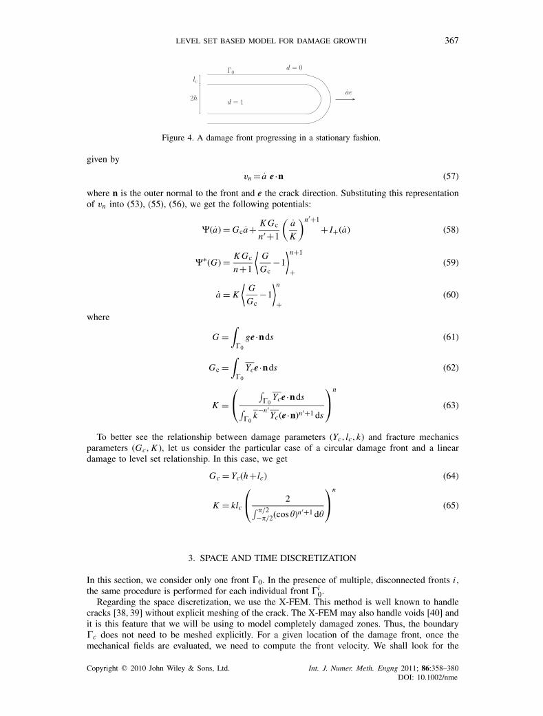
LEVEL SET BASED MODEL FOR DAMAGE GROWTH 367
Figure 4. A damage front progressing in a stationary fashion.
given by
vn = a e ·n (57)
where n is the outer normal to the front and e the crack direction. Substituting this representationof vn into (53), (55), (56), we get the following potentials:
�(a) = Gca+ K Gc
n′+1
(a
K
)n′+1
+ I+(a) (58)
�∗(G) = K Gc
n+1
⟨G
Gc−1
⟩n+1
+(59)
a = K
⟨G
Gc−1
⟩n
+(60)
where
G =∫
�0
ge·nds (61)
Gc =∫
�0
Yce ·nds (62)
K =⎛⎝ ∫
�0Yce ·nds∫
�0k−n′
Yc(e·n)n′+1 ds
⎞⎠n
(63)
To better see the relationship between damage parameters (Yc, lc,k) and fracture mechanicsparameters (Gc, K ), let us consider the particular case of a circular damage front and a lineardamage to level set relationship. In this case, we get
Gc = Yc(h+lc) (64)
K = klc
⎛⎝ 2∫ �/2
−�/2(cos)n′+1 d
⎞⎠n
(65)
3. SPACE AND TIME DISCRETIZATION
In this section, we consider only one front �0. In the presence of multiple, disconnected fronts i ,the same procedure is performed for each individual front �i
0.Regarding the space discretization, we use the X-FEM. This method is well known to handle
cracks [38, 39] without explicit meshing of the crack. The X-FEM may also handle voids [40] andit is this feature that we will be using to model completely damaged zones. Thus, the boundary�c does not need to be meshed explicitly. For a given location of the damage front, once themechanical fields are evaluated, we need to compute the front velocity. We shall look for the
Copyright � 2010 John Wiley & Sons, Ltd. Int. J. Numer. Meth. Engng 2011; 86:358–380DOI: 10.1002/nme
368 N. MOËS ET AL.
velocity on the front as a combination of modes:
vn =N∑
I=1vnI FI (66)
The modes FI are explicit functions of s initially defined on the front �0, then extended throughthe band �oc. The extension is performed just as a velocity is extended from the iso-zero of thelevel set when dealing with the level set equation [41, 42].
In order to find the velocity coefficients, the discretized expression of the velocity is introducedin (37)
infvn
∫�oc
�(d ′(�)vn)−Y d ′(�)vn d� (67)
The integration is restricted over �oc since outside this band d ′(�)=0. In the minimization, thevelocity vn must be positive. If the velocity is not positive the potential � is infinite. In order toimpose the positivity of the velocity, introduction of a Lagrange multiplier is useful.
infvn
sup�0
∫�c
�r (d ′(�)vn)−Y d ′(�)vn +d ′(�)vn d� (68)
where �r is the regular part of the potential � which is no longer infinite when the velocity isnegative. Note that in the above equation, the term also involves the gradient of the damage.This is important if we do not want to loose the constraint of positive velocity as lc goes to zero.The interpretation of the Lagrange multiplier is as follows: it will be zero in zones where the frontis moving and related to the gap Yc −Y in areas where it is not moving.
Finally, in order to remove the constraint �0 in (68) the trick, introduced for contact by BenDhia et al. [43], is to write
infvn
sup
∫�oc
�r (d ′(�)vn)−Y d ′(�)vn + d ′(�)
2�〈+�vn〉2
−− d ′(�)
2�2 d� (69)
where �>0 is a parameter that does not affect the solution. Differentiating with respect to vn and, we get∫
�oc
(��r (d ′(�)vn)
�vn+��d ′(�)vn
)�vn +�d ′(�)�vn d� =
∫�oc
Y d ′(�)�vn d� ∀�vn (70)
∫�oc
�d ′(�)vn�+(�−1)d ′(�)
��d� = 0 ∀� (71)
in which we did use the notation
�=�(,vn) = 0 if +�vn�0 (72)
�=�(,vn) = 1 if +�vn<0 (73)
This system may be solved using a Newton–Raphson technique. Two non-linearities appear.One coming from the constitutive law �r and the second coming from the contact condition �. Itwas shown in [43, 44] that solving one difficulty at a time was efficient. Basically, there are twoembedded loops in the Newton–Raphson procedure.
We now discretize
vn =N∑
I=1vnI FI , �vn =
N∑I=1
�vnI FI
=N∑
I=1I FI , �=
N∑I=1
�I FI
(74)
Copyright � 2010 John Wiley & Sons, Ltd. Int. J. Numer. Meth. Engng 2011; 86:358–380DOI: 10.1002/nme
LEVEL SET BASED MODEL FOR DAMAGE GROWTH 369
where the modes FI depend only on the curvilinear abscissa s⎡⎢⎣K i +�C0 C0
C0T C0 − M
�
⎤⎥⎦[
�vn
�
]=[
Ri
Si
](75)
K iI J =
∫�oc
�2�r (d ′(�)vin)
�2vn
FI FJ d� (76)
C0I J =
∫�oc
�0d ′(�)FI FJ d� (77)
MI J =∫
�oc
d ′(�)FI FJ d� (78)
RiI =
∫�oc
(−��r (d ′(�)vi
n)
�vn+Y d ′(�)+�0d ′(�)(i +�vi
n)
)FI d� (79)
SiI =
∫�oc
d ′(�)(�0(i/�+vin)−i/�)FI d� (80)
where �0 =�(0,v0n). We note that the velocity computation on the front does not require an explicit
computation of the configurational forces on the front.Regarding the loading, different types of control may be used. In the numerical experiments
we did use a crack mouth opening displacement (CMOD) for the three-point bending test and adissipation control-type algorithm for the other experiments. For the dissipation control algorithmwe were inspired by the work of Verhoosel et al. [45]. In our case, the dissipation reads as
D =∫
�oc
Y d ′(�)vn d� (81)
It is tempting to impose the value of D by some prescribed constants. Unfortunately at initiation,the left term goes to zero and the equality may only be satisfied for infinite loading. Hence, weintroduce a given parameter � and we take into account the volume of the damaged zone by theconstraint ∫
�oc
Y d ′(�)vn d�=∫
�oc
�d ′(�)d� (82)
This constraint is imposed through a Lagrange multiplier . Taking into account the dissipationconstraint, the inf–sup principle (69) now reads as
infvn
sup
sup
∫�oc
�r (d ′(�)vn)+ d ′(�)
2�〈+�vn〉2
−− d ′(�)
2�2 − Y0d ′(�)vn + log �d ′(�)d� (83)
where Y0 is the value of Y for a unit loading. It may be observed in the above that the meaning ofthe Lagrange parameter is simply the square of the loading. The corresponding Newton–Raphsoniteration is given below⎡
⎢⎢⎢⎢⎣K i +�C0 C0 D
C0T C0 − M
�0
DT 0 Ei
⎤⎥⎥⎥⎥⎦⎡⎢⎣
�vn
�
�
⎤⎥⎦=
⎡⎢⎢⎣
Ri
Si
T i
⎤⎥⎥⎦ (84)
Copyright � 2010 John Wiley & Sons, Ltd. Int. J. Numer. Meth. Engng 2011; 86:358–380DOI: 10.1002/nme
370 N. MOËS ET AL.
DI =∫
�oc
Y0d ′(�)FI d� (85)
Ei = −∫
�oc
�d ′(�)
i2d� (86)
T i =∫
�oc
(Y0d ′(�)vi
n − �d ′(�)
i
)d� (87)
Once the normal velocity of the level set is known, the level set may be updated using classicallevel set approaches [41, 42].
4. NUMERICAL SIMULATIONS FOR SEVERAL 2D CASES
In order to take into account more general loading cases and the closure effect in the fully damagedzone, we consider an asymmetric tension/compression damage potential with a scalar damagevariable. We have considered a strain-based model. Other types of models involving closure effectsmay be found in [46]
�(ε,d)=�(1−d)〈ε〉+ : 〈ε〉++�(1−hd)〈ε〉− : 〈ε〉−+
2(1−d)〈T rε〉2
++
2(1−hd)〈T rε〉2
− (88)
where and � are the Lamé elastic coefficients and h�1. The positive (negative) part of the tensoris applied to its spectral decomposition
〈ε〉+ =3∑
i=1〈εi 〉+ei ⊕ei (89)
〈ε〉− =3∑
i=1〈εi 〉−ei ⊕ei (90)
where εi , i =1,2,3, are the eigenvalues of the strain tensor and ei , i =1,2,3, the eigenvectors. Thepotential is expressed as follows using the eigenvalues (and plane strain assumption ε3 =0))
�(ε,d)= E
2(1+ )((1−�1d)ε2
1 +(1−�2d)ε22)+ E(1−�d)
2(1−2 )(1+ )(ε1 +ε2)2 (91)
with
�i = h if εi<0
1 if εi�0
� = h if ε1 +ε2<0
1 if ε1 +ε2�0
One can easily show that the eigenvectors of the stress and strain tensors coincide. The eigenstresses are obtained from the eigen strains by differentiating (91)(
�1
�2
)= E
1+
((1−�1d)+�(1−�d) �(1−�d)
�(1−�d) (1−�2d)+�(1−�d)
)︸ ︷︷ ︸
L
(ε1
ε2
)(92)
Storing the two eigen stresses in r and the two eigen strains in ε
r=Lε (93)
Copyright � 2010 John Wiley & Sons, Ltd. Int. J. Numer. Meth. Engng 2011; 86:358–380DOI: 10.1002/nme
LEVEL SET BASED MODEL FOR DAMAGE GROWTH 371
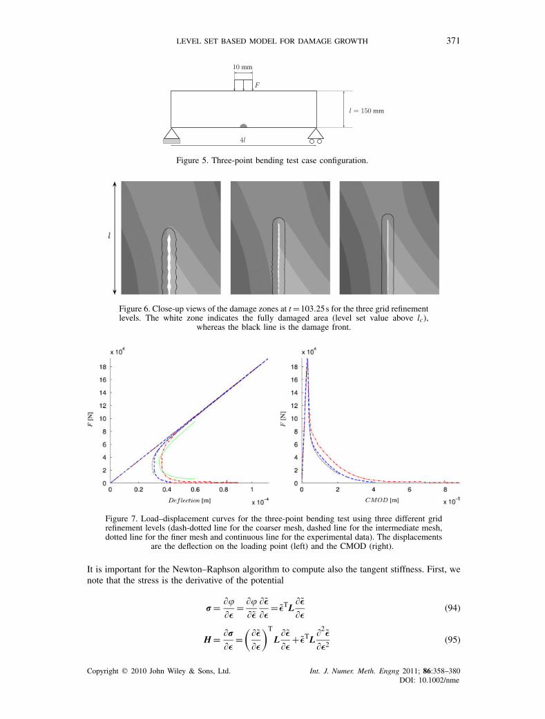
Figure 5. Three-point bending test case configuration.
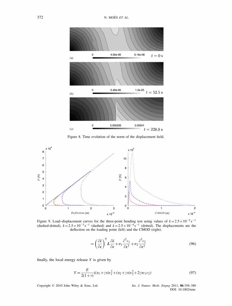
Figure 6. Close-up views of the damage zones at t =103.25s for the three grid refinementlevels. The white zone indicates the fully damaged area (level set value above lc),
whereas the black line is the damage front.
Figure 7. Load–displacement curves for the three-point bending test using three different gridrefinement levels (dash-dotted line for the coarser mesh, dashed line for the intermediate mesh,dotted line for the finer mesh and continuous line for the experimental data). The displacements
are the deflection on the loading point (left) and the CMOD (right).
It is important for the Newton–Raphson algorithm to compute also the tangent stiffness. First, wenote that the stress is the derivative of the potential
r= ��
�ε= ��
�ε�ε
�ε= εTL
�ε�ε
(94)
H = �r�ε
=(
�ε
�ε
)T
L�ε�ε
+ εTL�2
ε
�ε2(95)
Copyright � 2010 John Wiley & Sons, Ltd. Int. J. Numer. Meth. Engng 2011; 86:358–380DOI: 10.1002/nme
372 N. MOËS ET AL.
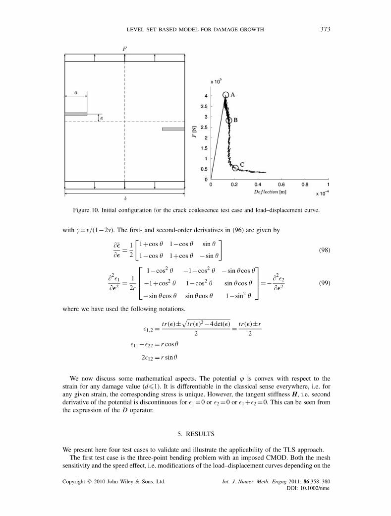
Figure 8. Time evolution of the norm of the displacement field.
Figure 9. Load–displacement curves for the three-point bending test using values of k =2.5×10⁻² s−1
(dashed-dotted), k =2.5×10⁻³ s−1 (dashed) and k =2.5×10⁻⁴ s−1 (dotted). The displacements are thedeflection on the loading point (left) and the CMOD (right).
=(
�ε
�ε
)T
L�ε
�ε+�1
�2ε1
�ε2+�2
�2ε2
�ε2(96)
finally, the local energy release Y is given by
Y = E
2(1+ )((�1 +��)ε2
1 +(�2 +��)ε22 +2��ε1ε2) (97)
Copyright � 2010 John Wiley & Sons, Ltd. Int. J. Numer. Meth. Engng 2011; 86:358–380DOI: 10.1002/nme
LEVEL SET BASED MODEL FOR DAMAGE GROWTH 373
Figure 10. Initial configuration for the crack coalescence test case and load–displacement curve.
with �= /(1−2 ). The first- and second-order derivatives in (96) are given by
�ε�ε
= 1
2
[1+cos 1−cos sin
1−cos 1+cos −sin
](98)
�2ε1
�ε2= 1
2r
⎡⎢⎢⎣
1−cos2 −1+cos2 −sin cos
−1+cos2 1−cos2 sin cos
−sin cos sin cos 1−sin2
⎤⎥⎥⎦=−�2
ε2
�ε2(99)
where we have used the following notations.
ε1,2 = tr (ε)±√
tr (ε)2 −4det(ε)
2= tr (ε)±r
2
ε11 −ε22 = r cos
2ε12 = r sin
We now discuss some mathematical aspects. The potential � is convex with respect to thestrain for any damage value (d�1). It is differentiable in the classical sense everywhere, i.e. forany given strain, the corresponding stress is unique. However, the tangent stiffness H, i.e. secondderivative of the potential is discontinuous for ε1 =0 or ε2 =0 or ε1 +ε2 =0. This can be seen fromthe expression of the D operator.
5. RESULTS
We present here four test cases to validate and illustrate the applicability of the TLS approach.The first test case is the three-point bending problem with an imposed CMOD. Both the mesh
sensitivity and the speed effect, i.e. modifications of the load–displacement curves depending on the
Copyright � 2010 John Wiley & Sons, Ltd. Int. J. Numer. Meth. Engng 2011; 86:358–380DOI: 10.1002/nme
374 N. MOËS ET AL.
Figure 11. Time evolution of the von Mises stress (left) and displacement norm fields (right).
ratio between the crack mouth opening velocity and the damage front velocity [47], are observedand the results are compared with a reference crack solution. The three remaining test cases illustratethe advantages of the method by considering the coalescence, branching and merging of crackswith an imposed dissipation rate to represent severe snap-backs on the load–displacement curves.
All computations are performed using a linear relationship d(�) and the non-linear potential(88). Note that this non-linearity does not have much impact on the solution for the three-pointbending problem since the damage zone essentially experiences traction. The dissipation potential
Copyright � 2010 John Wiley & Sons, Ltd. Int. J. Numer. Meth. Engng 2011; 86:358–380DOI: 10.1002/nme
LEVEL SET BASED MODEL FOR DAMAGE GROWTH 375
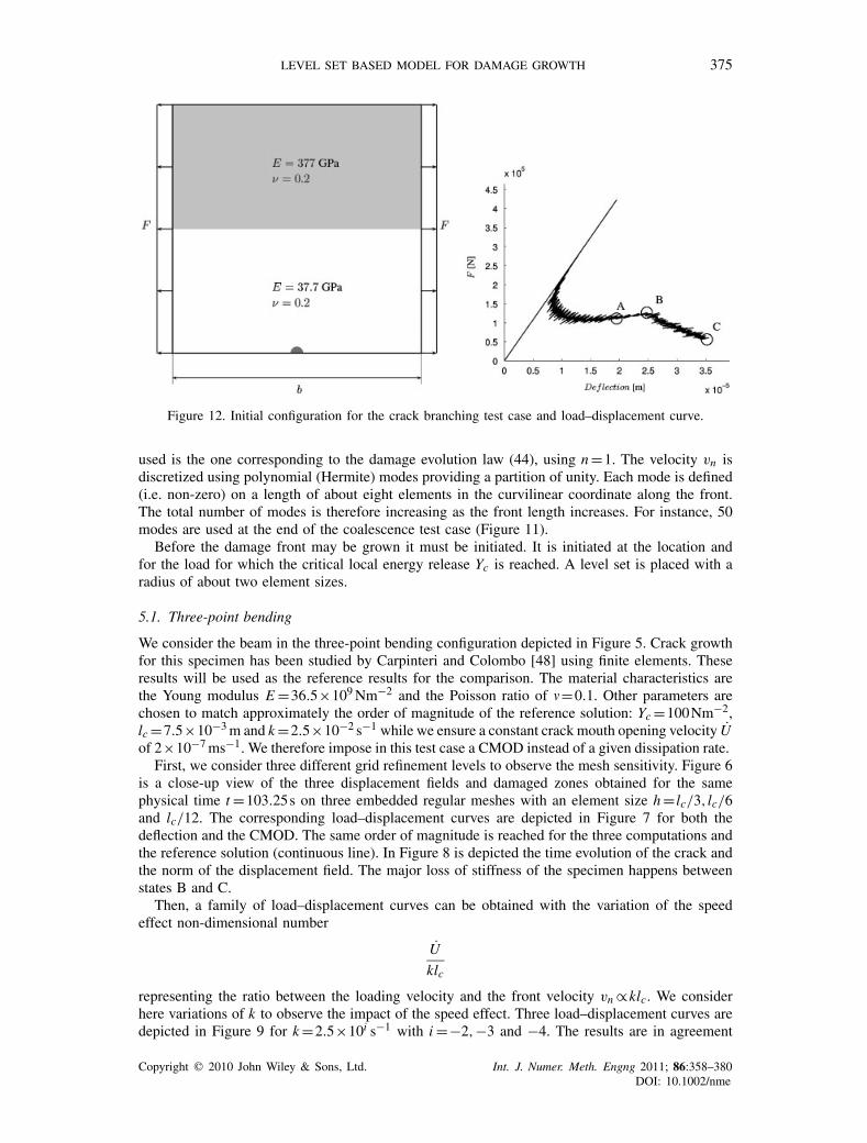
Figure 12. Initial configuration for the crack branching test case and load–displacement curve.
used is the one corresponding to the damage evolution law (44), using n =1. The velocity vn isdiscretized using polynomial (Hermite) modes providing a partition of unity. Each mode is defined(i.e. non-zero) on a length of about eight elements in the curvilinear coordinate along the front.The total number of modes is therefore increasing as the front length increases. For instance, 50modes are used at the end of the coalescence test case (Figure 11).
Before the damage front may be grown it must be initiated. It is initiated at the location andfor the load for which the critical local energy release Yc is reached. A level set is placed with aradius of about two element sizes.
5.1. Three-point bending
We consider the beam in the three-point bending configuration depicted in Figure 5. Crack growthfor this specimen has been studied by Carpinteri and Colombo [48] using finite elements. Theseresults will be used as the reference results for the comparison. The material characteristics arethe Young modulus E =36.5×10⁹ Nm−2 and the Poisson ratio of =0.1. Other parameters arechosen to match approximately the order of magnitude of the reference solution: Yc =100Nm−2,lc =7.5×10⁻³ m and k =2.5×10⁻² s−1 while we ensure a constant crack mouth opening velocity Uof 2×10⁻⁷ ms−1. We therefore impose in this test case a CMOD instead of a given dissipation rate.
First, we consider three different grid refinement levels to observe the mesh sensitivity. Figure 6is a close-up view of the three displacement fields and damaged zones obtained for the samephysical time t =103.25s on three embedded regular meshes with an element size h = lc/3, lc/6and lc/12. The corresponding load–displacement curves are depicted in Figure 7 for both thedeflection and the CMOD. The same order of magnitude is reached for the three computations andthe reference solution (continuous line). In Figure 8 is depicted the time evolution of the crack andthe norm of the displacement field. The major loss of stiffness of the specimen happens betweenstates B and C.
Then, a family of load–displacement curves can be obtained with the variation of the speedeffect non-dimensional number
U
klc
representing the ratio between the loading velocity and the front velocity vn ∝klc. We considerhere variations of k to observe the impact of the speed effect. Three load–displacement curves aredepicted in Figure 9 for k =2.5×10i s−1 with i =−2,−3 and −4. The results are in agreement
Copyright � 2010 John Wiley & Sons, Ltd. Int. J. Numer. Meth. Engng 2011; 86:358–380DOI: 10.1002/nme
376 N. MOËS ET AL.
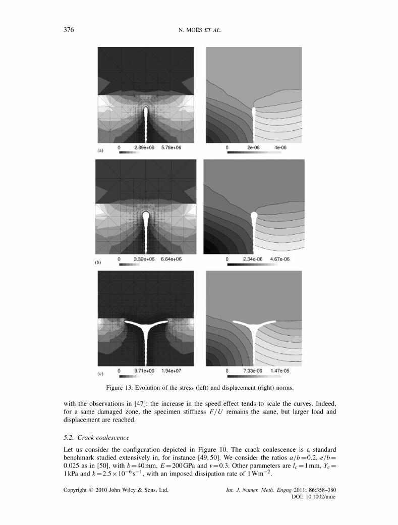
Figure 13. Evolution of the stress (left) and displacement (right) norms.
with the observations in [47]: the increase in the speed effect tends to scale the curves. Indeed,for a same damaged zone, the specimen stiffness F/U remains the same, but larger load anddisplacement are reached.
5.2. Crack coalescence
Let us consider the configuration depicted in Figure 10. The crack coalescence is a standardbenchmark studied extensively in, for instance [49, 50]. We consider the ratios a/b=0.2, e/b=0.025 as in [50], with b=40mm, E =200GPa and =0.3. Other parameters are lc =1mm, Yc =1kPa and k =2.5×10⁻⁶ s−1, with an imposed dissipation rate of 1Wm−2.
Copyright � 2010 John Wiley & Sons, Ltd. Int. J. Numer. Meth. Engng 2011; 86:358–380DOI: 10.1002/nme
LEVEL SET BASED MODEL FOR DAMAGE GROWTH 377
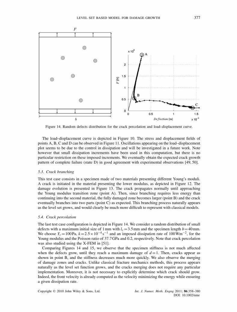
Figure 14. Random defects distribution for the crack percolation and load–displacement curve.
The load–displacement curve is depicted in Figure 10. The stress and displacement fields ofpoints A, B, C and D can be observed in Figure 11. Oscillations appearing on the load–displacementplot seems to be due to the control in dissipation and will be investigated in a future work. Notehowever that small dissipation increments have been used in this computation, but there is noparticular restriction on these imposed increments. We eventually obtain the expected crack growthpattern of complete failure (state D) in good agreement with experimental observations [49, 50].
5.3. Crack branching
This test case consists in a specimen made of two materials presenting different Young’s moduli.A crack is initiated in the material presenting the lower modulus, as depicted in Figure 12. Thedamage evolution is presented in Figure 13. The crack propagates normally until approachingthe Young modulus transition zone (point A). Then, since branching requires less energy thancontinuing into the second material, the fully damaged zone becomes larger (point B) and the crackeventually branches into two parts (point C) as expected. This branching process naturally appearsas the level set grows, and would clearly be much more difficult to represent with classical models.
5.4. Crack percolation
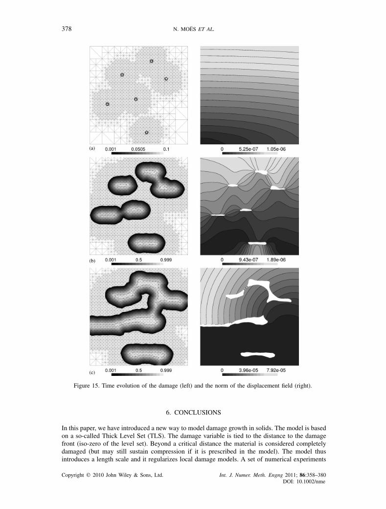
The last test case configuration is depicted in Figure 14. We consider a random distribution of smalldefects with a maximum initial size of 1mm with lc =3.5mm and the specimen length b=40mm.We choose Yc =100Pa, k =2.5×10⁻⁴ s−1 and an imposed dissipation rate of 100Wm−2, for theYoung modulus and the Poisson ratio of 37.7GPa and 0.2, respectively. Note that crack percolationwas also studied using the X-FEM in [51].
Comparing Figures 14 and 15, we observe that the specimen stiffness is not much affectedwhen the defects grow, until they reach a maximum damage of d =1. Then, cracks appear asshown in point B, and the stiffness decreases much more quickly. We also observe the mergingof damage zones and cracks. Unlike classical fracture mechanics methods, this process appearsnaturally as the level set function grows, and the cracks merging does not require any particularimplementation. Moreover, it is not necessary to explicitly determine which crack should grow.Indeed, the front velocity is already computed as the velocity minimizing the energy while ensuringa given dissipation rate.
Copyright � 2010 John Wiley & Sons, Ltd. Int. J. Numer. Meth. Engng 2011; 86:358–380DOI: 10.1002/nme
378 N. MOËS ET AL.
Figure 15. Time evolution of the damage (left) and the norm of the displacement field (right).
6. CONCLUSIONS
In this paper, we have introduced a new way to model damage growth in solids. The model is basedon a so-called Thick Level Set (TLS). The damage variable is tied to the distance to the damagefront (iso-zero of the level set). Beyond a critical distance the material is considered completelydamaged (but may still sustain compression if it is prescribed in the model). The model thusintroduces a length scale and it regularizes local damage models. A set of numerical experiments
Copyright � 2010 John Wiley & Sons, Ltd. Int. J. Numer. Meth. Engng 2011; 86:358–380DOI: 10.1002/nme
LEVEL SET BASED MODEL FOR DAMAGE GROWTH 379
did demonstrate the capability of the model to handle initiation, growth, branching and coalescenceof crack-like patterns.
ACKNOWLEDGEMENTS
The authors thank R. Desmorat and G. Pijaudier-Cabot for fruitful discussions. The reviewers are alsogratefully acknowledged for their accurate and constructive comments. Paul-Emile Bernard is a PostdoctoralResearcher supported by the Belgian National Fund for Scientific Research (FNRS). The support of theFondation FNRAE (Fondation Aéronautique et Espace) is also acknowledged.
REFERENCES
1. Kachanov L. Time of rupture process under creep conditions. Izvestiia Akademii Nauk SSSR, OtdelenieTekhmlchesikh Nauk 1958; 8:26–31.
2. Lemaitre J. A Course on Damage Mechanics. Springer: Berlin, 1992.3. Peerlings R. Gradient damage for quasi-brittle materials. Master Thesis, University of Eindhoven, 1994.4. Peerlings R, de Borst R, Brekelmans W, De Vree J. Gradient enhanced damage for quasi-brittle materials.
International Journal for Numerical Methods in Engineering 1996; 39:3391–3403.5. Bazant Z, Belytschko T, Chang T. Continuum theory fo strain-softening. Journal of Engineering Mechanics 1984;
110:1666–1692.6. Pijaudier-Cabot G, Bazant Z. Non-local damage theory. Journal of Engineering Mechanics 1987; 113:1512–1533.7. Aifantis E. On the structural origin of certain inelastic models. Journal of Engineering Materials and Technology
1984; 106:326–330.8. Triantafyllidis N, Aifantis E. A gradient approach to localization of deformation: I. Hyperelastic model. Journal
of Elasticity 1986; 16:225–237.9. Schreyer H, Chen Z. One-dimensional softening with localization. Journal of Applied Mechanics 1986; 53:
791–979.10. Mühlhaus H, Vardoulakis I. The thickness of shear bands in granular materials. Géotechnique 1987; 37:271–283.11. Fremond M, Nedjar B.Damage, gradient of damage and principle of virtual power. International Journal of
Solids and Structures 1996; 3(8):1083–1103.12. Pijaudier-Cabot G, Burlion N. Damage and localisation in elastic materials with voids. Mechanics of Cohesive-
frictional Materials 1996; 1:129–144.13. Nguyen QS, Andrieux S. The non-local generalized standard approach: a consistent gradient theory. Comptes
Rendus Académie des Sciences de Paris, Série II 2005; 333:139–145.14. Peerlings R, Geers M, de Borst R, Brekelmans W. A critical comparison of non-local and gradient-enhanced
softening continua. International Journal of Solids and Structures 2001; 38(44–45):7723–7746.15. Hakim V, Karma A. Laws of crack motion and phase-field models of fracture. Journal of Mechanics and Physics
of Solids 2009; 57(2):342–368.16. Hakim V, Karma A. Crack path prediction in anisotropic brittle materials. Physical Review Letters 2005;
95:235501.17. Karma A, Kessler D, Levine H. Phase field of mode III dynamic fracture. Physical Review Letters 2001;
8704:045501.18. Francfort GA, Marigo J-J. Revisiting brittle fracture as an energy minimization problem. Journal of Mechanics
and Physics of Solids 1998; 46(8):1319–1342.19. Bourdin B, Francfort GA, Marigo J-J. Numerical experiments in revisited brittle fracture. Journal of Mechanics
and Physics of Solids 2000; 48(4):797–826.20. Bourdin B, Francfort GA, Marigo J-J. The variational approach to fracture. Journal of Elasticity 2008; 91:5–148.21. Allaire G, Van Goethem N, Jouve F. A level set method for the numerical simulation of damage evolution,
Technical Report, 629, Note École Polytechnique, Centre de Mathématiques Appliquées, 2007.22. Pradeilles-Duval RM, Stolz C. On the evolution of solids in the presence of irreversible phase transformation.
Comptes Rendus Académie des Sciences de Paris, Série II 1991; 313(3):297–302.23. Pradeilles-Duval RM, Stolz C. Mechanical transformations and discontinuities along a moving surface. Journal
of Mechanics and Physics of Solids 1995; 43(1):91–121.24. Moës N, Chevaugeon N, Dufour F. A Regularized Brittle Damage Model Solved by a Level Set Technique,
IUTAM Book Series, Cape Town, South Africa, 2008.25. Nguyen QS, Pradeilles RM, Stolz C. Sur une loi régularisante en rupture et endommagement fragile. Comptes
Rendus Académie des Sciences de Paris, Série II 1989; 309:1515–1520.26. Stolz C. Bifurcation of equilibrium solutions and defects nucleation. International Journal of Fracture 2007;
147:103–107.27. Salac D, Lu W. A level set approach to model directed nanocrack patterns. Computer Material Sciences 2007;
39(4):849–856.28. Simone A, Wells GN, Sluys LJ. From continuous to discontinuous failure in a gradient-enhanced continuum
damage model. Computer Methods in Applied Mechanics and Engineering 2003; 192(41–42):4581–4607.
Copyright � 2010 John Wiley & Sons, Ltd. Int. J. Numer. Meth. Engng 2011; 86:358–380DOI: 10.1002/nme
380 N. MOËS ET AL.
29. Simone A, Sluys LJ. The use of displacement discontinuities in a rate-dependent medium. Computer Methodsin Applied Mechanics and Engineering 2004; 193(27–29):3015–3033.
30. Comi C, Mariani S, Perego U. An extended FE strategy for transition from continuum damage to mode Icohesive crack propagation. International Journal for Numerical Analysis and Methods in Geomechanics 2007;31(2):213–238.
31. Saanouni K, Belamri N, Autesserre P. Finite element simulation of 3D sheet metal guillotining using advanced fullycoupled elastoplastic-damage constitutive equations. Finite Elements in Analysis and Design 2010; 46(7):535–550.
32. Mazars J, Pijaudier-Cabot G. From damage to fracture and conversely: a combined approach. InternationalJournal of Solids and Structures 1996; 33(20–22):3327–3342.
33. Stolz C. On the propagation of discontinuity and shock generating function in anelastic solids mechanics. ComptesRendus Académie des Sciences de Paris, Série II 1989; 308:1–3.
34. Stolz C. Thermodynamical description of running discontinuities. In Continuum Thermodynamics, Maugin GAet al. (eds). Kluwer Academic Publishers: Dordrecht, 2000; 401–412.
35. Dequiedt JL, Stolz C. Propagation of shock discontinuity in an elasto-plastic materials: constituitve relations.Archives of Mechanics 2004; 56:5.
36. Lorentz E, Andrieux S. Analysis of non-local models through energetic formulations. International Journal ofSolids and Structures 2003; 40(12):2905–2936.
37. Simone A, Askes H, Sluys LJ. Incorrect initiation and propagation of failure in non-local and gradient-enhancedmedia. International Journal of Solids and Structures 2004; 41:351–363.
38. Moës N, Dolbow J, Belytschko T. A finite element method for crack growth without remeshing. InternationalJournal for Numerical Methods in Engineering 1999; 46(1):131–150.
39. Belytschko T, Moës N, Usui S, Parimi C. Arbitrary discontinuities in finite elements. International Journal forNumerical Methods in Engineering 2001; 50(4):993–1013.
40. Daux C, Moës N, Dolbow J, Sukumar N, Belytschko T. Arbitrary branched and intersecting cracks withthe eXtended finite element method. International Journal for Numerical Methods in Engineering 2000; 48:1741–1760.
41. Sethian JA. Level Set Methods and Fast Marching Method: Evolving Interfaces in Computational Geometry,Fluid Mechanics, Computer Vision, and Materials Science. Cambridge University Press: Cambridge, 1999.
42. Osher S, Fedkiw R. Level Set Methods and Dynamic Implicit Surfaces. Springer: Berlin, 2002.43. Ben Dhia H, Vautier I, Zarroug M. Problèmes de contact frottant en grandes transformations: du continu au
discret. Revue Européenne des Éléments Finis 2000; 9:243–261.44. Zarroug M. Eléments Mixtes de Contact Frottant en Grandes Transformation et Applications. Ecole Centrale de
Paris, 2002.45. Verhoosel CV, Remmers JJC, Gutiérrez MA. A dissipation-based arc-length method for robust simulation of
brittle and ductile failure. International Journal for Numerical Methods in Engineering 2009; 77:9.46. Lemaitre J, Desmorat R. Engineering Damage Mechanics: Ductile, Creep, Fatigue and Brittle Failures. Springer:
Berlin, 2005.47. Bazant ZP, Gettu R. Rate effects and load relaxation in static fracture of concrete. ACI Materials Journal 1992;
89(5):456–468.48. Carpinteri A, Colombo G. Numerical analysis of catastrophic softening behavior (snap-back instability). Computers
and Structures 1989; 31:607–636.49. Melin S. Why do cracks avoid each other. International Journal of Fracture 1983; 23(1):37–45.50. Sumi Y, Wang ZN. A finite-element simulation method for a system of growing cracks in a heterogeneous
materials. Mechanics of Materials 1998; 28:197–206.51. Budyn E, Zi G, Moës N, Belytschko T. A model for multiple crack growth in brittle materials without remeshing.
International Journal for Numerical Methods in Engineering 2004; 61:10.
Copyright � 2010 John Wiley & Sons, Ltd. Int. J. Numer. Meth. Engng 2011; 86:358–380DOI: 10.1002/nme


![Narrow Band Level set on GPU - Kentzwang/schedule/zq9_1.pdfImplicit Contour: Level-set [1]S. Osher and R.P. Fedkiw, Level set methods and dynamic implicit surfaces, Springer, 2003](https://img.pdfslide.net/doc/110x75/5f08e0bb7e708231d42428b4/narrow-band-level-set-on-gpu-zwangschedulezq91pdf-implicit-contour-level-set.jpg)