Commun Nonlinear Sci Numer Simulat 19 (2014) 3149–3160

Contents lists available at ScienceDirect

Commun Nonlinear Sci Numer Simulat

journal homepage: www.elsevier .com/locate /cnsns

A mathematical model for a distributed attack on targetedresources in a computer network

http://dx.doi.org/10.1016/j.cnsns.2014.01.0281007-5704/� 2014 Elsevier B.V. All rights reserved.

⇑ Corresponding author. Tel.: +91 9430764860; fax: +91 651 2275401.E-mail addresses: haldarkaushik@gmail.com (K. Haldar), drbimalmishra@gmail.com (B.K. Mishra).

Kaushik Haldar, Bimal Kumar Mishra ⇑Department of Applied Mathematics, Birla Institute of Technology, Mesra, Ranchi 835 215, India

a r t i c l e i n f o a b s t r a c t

Article history:Received 11 May 2013Received in revised form 28 January 2014Accepted 31 January 2014Available online 8 February 2014

Keywords:Epidemic modelsTargeted attackDistributed attackStability

A mathematical model has been developed to analyze the spread of a distributed attack oncritical targeted resources in a network. The model provides an epidemic framework withtwo sub-frameworks to consider the difference between the overall behavior of the attack-ing hosts and the targeted resources. The analysis focuses on obtaining threshold condi-tions that determine the success or failure of such attacks. Considering the criticality ofthe systems involved and the strength of the defence mechanism involved, a measurehas been suggested that highlights the level of success that has been achieved by theattacker. To understand the overall dynamics of the system in the long run, its equilibriumpoints have been obtained and their stability has been analyzed, and conditions for theirstability have been outlined.

� 2014 Elsevier B.V. All rights reserved.

1. Introduction

The use of distributed attacking methods helps the perpetrators of a malicious attack in a computer network to multiplythe strength of the attack by utilizing a number of attacking hosts for launching and propagating the attack. The most pop-ular among such attacks is the Distributed Denial of Service (DDoS) attack, where a number of attackers generate flooding traf-fic, which is directed from multiple sources, towards a set of selected nodes or a range of IP addresses in the Internet. Suchattacks may employ different methodologies, but the underlying basic principle is to overwhelm a target node with a mas-sive rate of incoming useless packets, and thereby to exhaust the resources that were available to serve legitimate users [1].A DDoS attack uses a number of compromised hosts to attack target computers simultaneously. A number of attempts havebeen made to mathematically understand and analyze such attacks [1,2]. However, the relation between distributed modesof attack and between targeted attacks remains to be explored, particularly considering the fact that targeted attacks arenow becoming much more frequent, and the criticality of the targets selected is also increasing. According to Symantec re-ports, the global average of reported targeted attacks has increased from 77 in 2010, to 82 in 2011, and then to 116 in 2012[3,4]. One of the most famous targeted attacks was the Stuxnet attack, which was witnessed in 2010 [5]. It became one of themost noticed attacks because of its main motive of cyber sabotage, where it showed that targeted attacks could cause damageto physical resources. It was a worm with an advanced payload that targeted systems responsible for controlling and mon-itoring industrial processes. It led to strong suspicion that it was meant to target nuclear installations in Iran. In 2011, a var-iation of Stuxnet, called Duqu, came into prominence [6]. Some other targeted attacks against the sensitive petroleum andchemical industries were also observed subsequently. Attackers are now using specialized intrusion techniques and tools

3150 K. Haldar, B.K. Mishra / Commun Nonlinear Sci Numer Simulat 19 (2014) 3149–3160

which are highly customized to carry out targeted attacks. To reduce the detection risk, stealthy methods with patience andpersistence are being developed and used. Such attacks are increasingly becoming better supported, better financed and bet-ter staffed, often having the backing of military or intelligence bodies of national governments. More and more of these at-tacks are being targeted against strategically important bodies including government agencies, military and defenseinstitutions, economic forums, and controllers of other critical infrastructure. Table 1 in Appendix A highlights some ofthe most popular targeted attacks over the last 5 years.

In this paper we try to analyze the impact of distributed attacks on critical targeted resources and try to obtain mathe-matical conditions for the success or failure of such attacks in causing substantial damage to the resources. We make a dis-tinction between the targeted resources and the hosts used to launch the distributed form of attack. An epidemic model isproposed that considers a unidirectional transmission of infection from identified hosts towards the targeted systems. Themodel tries to consider both the malicious intentions of identifying new hosts for spreading the attack as well as damaging asmany targets as possible. Unlike most epidemiology based approaches, the targeted systems in our model do not participatein spreading the attack in either population. Further, there is no consideration of addition of nodes into the targeted popu-lation, which allows us to highlight the criticality of the scenario being modeled. We have obtained an analytical thresholdon which the behavior of the modeled system depends. In Section 2, a mathematical formulation of the model is obtained.Section 3 discusses some of the preliminary results governing the long term behavior of the system, while Section 4 provesthe global stability of an endemic equilibrium point for the system, where the impact of the attack is seen to persist in boththe populations. Section 5 finally concludes the paper.

2. Mathematical model

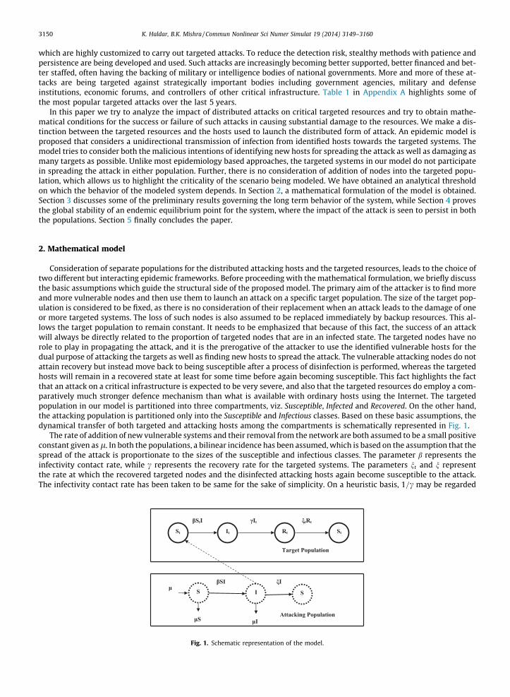
Consideration of separate populations for the distributed attacking hosts and the targeted resources, leads to the choice oftwo different but interacting epidemic frameworks. Before proceeding with the mathematical formulation, we briefly discussthe basic assumptions which guide the structural side of the proposed model. The primary aim of the attacker is to find moreand more vulnerable nodes and then use them to launch an attack on a specific target population. The size of the target pop-ulation is considered to be fixed, as there is no consideration of their replacement when an attack leads to the damage of oneor more targeted systems. The loss of such nodes is also assumed to be replaced immediately by backup resources. This al-lows the target population to remain constant. It needs to be emphasized that because of this fact, the success of an attackwill always be directly related to the proportion of targeted nodes that are in an infected state. The targeted nodes have norole to play in propagating the attack, and it is the prerogative of the attacker to use the identified vulnerable hosts for thedual purpose of attacking the targets as well as finding new hosts to spread the attack. The vulnerable attacking nodes do notattain recovery but instead move back to being susceptible after a process of disinfection is performed, whereas the targetedhosts will remain in a recovered state at least for some time before again becoming susceptible. This fact highlights the factthat an attack on a critical infrastructure is expected to be very severe, and also that the targeted resources do employ a com-paratively much stronger defence mechanism than what is available with ordinary hosts using the Internet. The targetedpopulation in our model is partitioned into three compartments, viz. Susceptible, Infected and Recovered. On the other hand,the attacking population is partitioned only into the Susceptible and Infectious classes. Based on these basic assumptions, thedynamical transfer of both targeted and attacking hosts among the compartments is schematically represented in Fig. 1.

The rate of addition of new vulnerable systems and their removal from the network are both assumed to be a small positiveconstant given as l. In both the populations, a bilinear incidence has been assumed, which is based on the assumption that thespread of the attack is proportionate to the sizes of the susceptible and infectious classes. The parameter b represents theinfectivity contact rate, while c represents the recovery rate for the targeted systems. The parameters nt and n representthe rate at which the recovered targeted nodes and the disinfected attacking hosts again become susceptible to the attack.The infectivity contact rate has been taken to be same for the sake of simplicity. On a heuristic basis, 1=c may be regarded

Fig. 1. Schematic representation of the model.

K. Haldar, B.K. Mishra / Commun Nonlinear Sci Numer Simulat 19 (2014) 3149–3160 3151

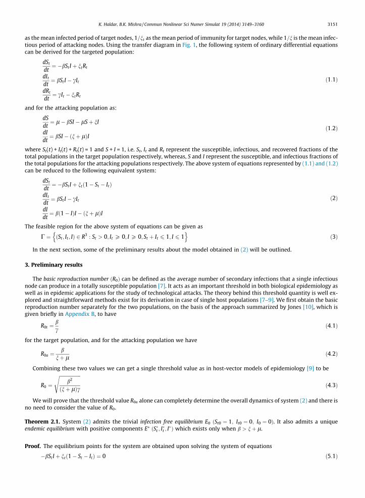
as the mean infected period of target nodes, 1=nt as the mean period of immunity for target nodes, while 1=n is the mean infec-tious period of attacking nodes. Using the transfer diagram in Fig. 1, the following system of ordinary differential equationscan be derived for the targeted population:

dSt

dt¼ �bStI þ ntRt

dIt

dt¼ bStI � cIt

dRt

dt¼ cIt � ntRt

ð1:1Þ

and for the attacking population as:

dSdt¼ l� bSI � lSþ nI

dIdt¼ bSI � ðnþ lÞI

ð1:2Þ

where St(t) + It(t) + Rt(t) = 1 and S + I = 1, i.e. St, It and Rt represent the susceptible, infectious, and recovered fractions of thetotal populations in the target population respectively, whereas, S and I represent the susceptible, and infectious fractions ofthe total populations for the attacking populations respectively. The above system of equations represented by (1.1) and (1.2)can be reduced to the following equivalent system:

dSt

dt¼ �bStI þ ntð1� St � ItÞ

dIt

dt¼ bStI � cIt

dIdt¼ bð1� IÞI � ðnþ lÞI

ð2Þ

The feasible region for the above system of equations can be given as

C ¼ ðSt; It ; IÞ 2 R3 : St > 0; It P 0; I P 0; St þ It 6 1; I 6 1n o

ð3Þ

In the next section, some of the preliminary results about the model obtained in (2) will be outlined.

3. Preliminary results

The basic reproduction number ðR0Þ can be defined as the average number of secondary infections that a single infectiousnode can produce in a totally susceptible population [7]. It acts as an important threshold in both biological epidemiology aswell as in epidemic applications for the study of technological attacks. The theory behind this threshold quantity is well ex-plored and straightforward methods exist for its derivation in case of single host populations [7–9]. We first obtain the basicreproduction number separately for the two populations, on the basis of the approach summarized by Jones [10], which isgiven briefly in Appendix B, to have

R0t ¼bc

ð4:1Þ

for the target population, and for the attacking population we have

R0a ¼b

nþ lð4:2Þ

Combining these two values we can get a single threshold value as in host-vector models of epidemiology [9] to be

R0 ¼

ffiffiffiffiffiffiffiffiffiffiffiffiffiffiffiffiffiffib2

ðnþ lÞc

sð4:3Þ

We will prove that the threshold value R0a alone can completely determine the overall dynamics of system (2) and there isno need to consider the value of R0.

Theorem 2.1. System (2) admits the trivial infection free equilibrium E0 ðSt0 ¼ 1; It0 ¼ 0; I0 ¼ 0Þ. It also admits a uniqueendemic equilibrium with positive components E⁄ ðS�t ; I

�t ; I�Þ which exists only when b > nþ l.

Proof. The equilibrium points for the system are obtained upon solving the system of equations

�bStI þ ntð1� St � ItÞ ¼ 0 ð5:1Þ

3152 K. Haldar, B.K. Mishra / Commun Nonlinear Sci Numer Simulat 19 (2014) 3149–3160

bStI � cIt ¼ 0 ð5:2Þ

bð1� IÞI � ðnþ lÞI ¼ 0 ð5:3Þ

where Eq. (5.3) gives the two values of I to be I0 = 0 and I⁄ = b�n�lb . h

Using the other two equations and the value I0 = 0, the trivial infection free equilibrium is found at the point E0

ðSt0003D1; It0 ¼ 0; I0 ¼ 0Þ. The other value I⁄ clearly exists only when b > nþ l, and in this case the equilibrium point isobtained at

S�t ¼nt

nt þ 1þ ntc

� �ðb� n� lÞ

I�t ¼nt

ntcb�n�lþ ðcþ ntÞ

I� ¼ b� n� lb

ð6Þ

This equilibrium point has a positive component of infection, provided the given condition is satisfied.

Theorem 2.2. The infection free equilibrium E0 of system (2) is locally asymptotically stable in C if R0a < 1 and is unstable ifR0a > 1.

Proof. Linearizing system (2) around the infection free equilibrium E0 (1,0,0), we get the following Jacobian matrix

JIFE ¼�nt �nt �b

0 �c b

0 0 b� ðnþ lÞ

264

375 ð7:1Þ

h

The characteristic equation for this matrix is given as

ðkþ ntÞðkþ cÞðk� bþ nþ lÞ ¼ 0 ð7:2Þ

and hence the characteristic roots are k1 ¼ �nt < 0; k2 ¼ �c < 0 and k3 ¼ b� ðnþ lÞ where k1 and k2 are both negative. Thethird eigen value k3 also becomes negative when the condition b < nþ l is satisfied, which is equivalent to the condition thatR0a < 1. Thus all the eigen values of the Jacobian matrix are negative in this case, and hence the infection free equilibrium islocally asymptotically stable. On the other hand when R0a > 1, i.e. b > nþ l, then k3 is positive and so the equilibrium pointbecomes unstable.

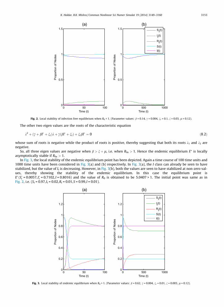
In Fig. 2, a numerical simulation has been used to depict this scenario graphically. The figure shows that the infection freeequilibrium point is locally stable. Here we have taken the initial point to be (St = 0.97, It = 0.02, Rt = 0.01, S = 0.99, I = 0.01)and it can be clearly observed that the equilibrium point E0 ðSt0 ¼ 1; It0 ¼ 0; I0 ¼ 0Þ turns out to be stable and in this case thevalue of R0 is calculated to be 0.9333 < 1. In Fig. 2(a), a time range of 100 time units has been considered, and in this case theattack is seen to be spreading. However, in Fig. 2(b), where a longer time interval of 1000 units has been considered, it can beseen that the infection was not able to spread as expected from the initial observations of Fig. 2(a), but rather it disappearedover a period of time, thereby showing that the point E0 is stable.

Theorem 2.3. The endemic equilibrium E⁄ is locally asymptotically stable in the interior of C if R0a > 1.

Proof. Proceeding similarly as in Theorem 2.2, the system is linearized at the endemic equilibrium E⁄ to get the Jacobianmatrix

JEE ¼�bI� � nt �nt �bS�t

bI� �c bS�t0 0 �2bI� þ b� ðnþ lÞ

264

375 ð8:1Þ

h

One of the eigen values is given as

k3 ¼ �2bI� þ b� ðnþ lÞ

which on simplification becomes k3 ¼ �ðb� n� lÞ < 0 if b > nþ l or equivalently R0a > 1.

0 50 1000

0.5

1

1.5

Time (t)

Pro

porti

on o

f Nod

es

(a)

0 500 10000

0.5

1

1.5

Time (t)P

ropo

rtion

of N

odes

(b)St(t)

It(t)

Rt(t)

S(t)I(t)

Fig. 2. Local stability of infection free equilibrium when R0 < 1. (Parameter values: b = 0.14, c = 0.004, nt = 0.1, n = 0.03, l = 0.12).

K. Haldar, B.K. Mishra / Commun Nonlinear Sci Numer Simulat 19 (2014) 3149–3160 3153

The other two eigen values are the roots of the characteristic equation

k2 þ ðcþ bI� þ ntÞkþ cðbI� þ ntÞ þ ntbI� ¼ 0 ð8:2Þ

whose sum of roots is negative while the product of roots is positive, thereby suggesting that both its roots k1 and k2 arenegative.

So, all three eigen values are negative when b > nþ l, i.e. when R0a > 1. Hence the endemic equilibrium E⁄ is locallyasymptotically stable if R0a > 1.

In Fig. 3, the local stability of the endemic equilibrium point has been depicted. Again a time course of 100 time units and1000 time units have been considered in Fig. 3(a) and (b) respectively. In Fig. 3(a), the I class can already be seen to havestabilized, but the value of It is decreasing. However, in Fig. 3(b), both the values are seen to have stabilized at non-zero val-ues, thereby showing the stability of the endemic equilibrium. In this case the equilibrium point isE�ðS�t = 0.0057, I�t = 0.7102, I = 0.8016) and the value of R0 is obtained to be 5.0407 > 1. The initial point was same as inFig. 2, i.e. (St = 0.97, It = 0.02,Rt = 0.01,S = 0.99, I = 0.01).

0 50 1000

0.2

0.4

0.6

0.8

1

1.2

Time (t)

Pro

porti

on o

f Nod

es

(a)

0 500 10000

0.2

0.4

0.6

0.8

1

1.2

Time (t)

Pro

porti

on o

f Nod

es

(b)

St(t)

It(t)

Rt(t)

S(t)I(t)

Fig. 3. Local stability of endemic equilibrium when R0 > 1. (Parameter values: b = 0.62, c = 0.004, nt = 0.01, n = 0.003, l = 0.12).

3154 K. Haldar, B.K. Mishra / Commun Nonlinear Sci Numer Simulat 19 (2014) 3149–3160

In the next section, we explore the global stability of the endemic equilibrium. Mathematically, for two-dimensional epi-demic systems, the Poincare–Bendixson trichotomy allows a useful method for the analysis of global asymptotic stability ofthe endemic equilibrium. The analysis becomes more complicated for the study of systems with n larger than 2. A majorbreakthrough was obtained in the nineties when Li and Muldowney suggested a geometric approach to global stability, wherethey generalized the Poincare–Bendixson criteria [11]. This approach has been used extensively in the analysis of globalbehavior of numerous epidemic models and in this paper also this method will be used.

4. Global stability of endemic equilibrium

In this section, the global stability analysis of the endemic equilibrium E⁄ will be done using the geometric approach sug-gested by Li and Muldowney [11], which has been summarized briefly in Appendix C. The sufficient conditions for the globalstability of the equilibrium point are shown to be (H1) and (H2) along with the Bendixson criteria given in Theorem C.1. Thesystem (2) satisfies conditions (H1) and (H2) under the assumption in Theorem 2.3. Using the instability of the infection freeequilibrium, shown in Theorem 2.2, we infer the uniform persistence of the system [12], which means that there exists apositive constant c, such that for any initial point ðStð0Þ; Itð0Þ; Ið0ÞÞ lying in the interior of C any solution ðStðtÞ; ItðtÞ; IðtÞÞsatisfies

min limt!1

inf StðtÞ; limt!1

inf ItðtÞ; limt!1

inf IðtÞn o

> c ð9Þ

Condition (9) along with the boundedness of C is equivalent to the existence of a compact absorbing set K in the interiorof C ([13]). This verifies condition (H1) and also condition (H2) follows from the fact that E⁄ is the only equilibrium point inthe interior of C.

Theorem 4.1. The unique endemic equilibrium point E⁄ is globally asymptotically stable in the interior of C if R0 > 1.

Proof. For a general solution ðStðtÞ; ItðtÞ; IðtÞÞ of system (2), the Jacobian matrix is

J ¼�bI � nt �nt �bSt

bI �c bSt

0 0 �2bI þ b� ðnþ lÞ

264

375 ð10Þ

h

Using (B.4), its second additive compound matrix J[2] is

J½2� ¼�bI � nt � c bSt bSt

0 �3bI � nt þ b� n� l �nt

0 bI �cþ b� 2bI � n� l

264

375 ð11Þ

Let the function P ¼ PðSt ; It; IÞ be defined as

P ¼ PðSt ; It ; IÞ ¼1 0 00 It

I 0

0 0 ItI

264

375 ¼ diag 1;

It

I;It

I

� �ð12Þ

Then

Pf P�1 ¼

0 0 00 I0t

It� I0

I 0

0 0 I0tIt� I0

I

2664

3775 ð13Þ

and

PJ½2�P�1 ¼�bI � nt � c bSt I

It

bSt IIt

0 �3bI � nt þ b� n� l �nt

0 bI �cþ b� 2bI � n� l

2664

3775 ð14Þ

So, we have

B ¼ Pf P�1 þ PJ½2�P�1 ¼

B11 B12

B21 B22

� �

K. Haldar, B.K. Mishra / Commun Nonlinear Sci Numer Simulat 19 (2014) 3149–3160 3155

where the elements of the block matrix B are

B11 ¼ ½�bI � nt � c�

B12 ¼ bSt IIt

bSt IIt

h i

B21 ¼00

� �

B22 ¼�3bI � nt þ b� n� lþ I0t

It� I0

I �nt

bI �cþ b� 2bI � n� lþ I0tIt� I0

I

24

35

Next for a vector (u,v,w) in R3, we select a norm as

jðu; v;wÞj ¼maxfjuj; jv þwjg ð15Þ

and denote by l the Lozinskii measure for this norm.From [13], it follows that

lðBÞ 6 supfg1; g2g ð16Þ

where g1 and g2 are defined as follows

g1 ¼ l1ðB11Þ þ jB12j ð17:1Þ

g2 ¼ jB21j þ l1ðB22Þ ð17:2Þ

Here jB12j and jB21j are matrix norms with respect to the L1 vector norm and l1 denotes the Lozinskii measure with re-spect to the L1 norm. So, we have

l1ðB11Þ ¼ �bI � nt � c ð18:1Þ

jB812j ¼bStI

Itð18:2Þ

jB821j ¼ 0 ð18:3Þ

l1ðB22Þ ¼ max �2bI � nt þ b� n� lþ I0tIt� I0

I;�2bI � nt þ b� n� l� cþ I0t

It� I0

I

� �

¼ �2bI � nt þ b� n� lþ I0tIt� I0

Ið18:4Þ

where the value of l1ðB22Þ has been calculated by taking the maximum of the two sums obtained by adding the absolutevalue of the non-diagonal in a column with the diagonal element in that column.

Putting the values from (18.1)–(18.4) in (17.1) and (17.2), we get

g1 ¼ �bI � nt � cþ bStIIt

ð19:1Þ

g2 ¼ �2bI � nt þ b� n� lþ I0tIt� I0

Ið19:2Þ

From (2), the equations can be rewritten as

I0tItþ c ¼ bStI

Itð20:1Þ

I0

I¼ b� bI � n� l ð20:2Þ

Substituting the values from (20.1) and (20.2) in (19.1) and (19.2) respectively, gives

g1 ¼ �bI � nt þI0tIt6

I0tIt� nt ð21:1Þ

g2 ¼ �bI � nt þI0

Iþ I0t

It� I0

I6

I0tIt� nt ð21:2Þ

0 0.1 0.2 0.3 0.4 0.5 0.6 0.7 0.8 0.9 10

0.1

0.2

0.3

0.4

0.5

0.6

0.7

0.8

0.9

1

Proportion of nodes in St class

Pro

porti

on o

f nod

es in

I t c

lass

Fig. 4. Global stability of endemic equilibrium when R0 > 1. (Parameter values: b = 0.62, c = 0.004, nt = 0.01, n = 0.003, l = 0.12).

3156 K. Haldar, B.K. Mishra / Commun Nonlinear Sci Numer Simulat 19 (2014) 3149–3160

Hence, from (16)

lðBÞ 6 I0tIt� nt

and so

1t

Z t

0lðBÞds 6

1t

logeItðtÞItð0Þ

� nt :

Hence, �q2 < 0, and so the Bendixson criteria is also fulfilled, thereby proving the global stability of the endemicequilibrium.

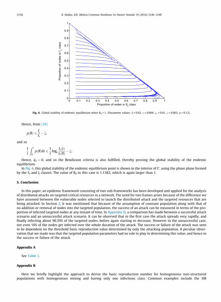
In Fig. 4, this global stability of the endemic equilibrium point is shown in the interior of C, using the phase plane formedby the St and It classes. The value of R0 in this case is 1.1382, which is again larger than 1.

5. Conclusion

In this paper, an epidemic framework consisting of two sub-frameworks has been developed and applied for the analysisof distributed attacks on targeted critical resources in a network. The need for two frames arises because of the difference wehave assumed between the vulnerable nodes selected to launch the distributed attack and the targeted resources that arebeing attacked. In Section 2, it was mentioned that because of the assumption of constant population along with that ofno addition or removal of nodes into the targeted population, the success of an attack can be measured in terms of the pro-portion of infected targeted nodes at any instant of time. In Appendix D, a comparison has made between a successful attackscenario and an unsuccessful attack scenario. It can be observed that in the first case the attack spreads very rapidly, andfinally infecting about 90.39% of the targeted nodes, before again starting to decrease. However in the unsuccessful case,not even 10% of the nodes get infected over the whole duration of the attack. The success or failure of the attack was seento be dependent on the threshold basic reproduction value determined by only the attacking population. A peculiar obser-vation that we made was that the targeted population parameters had no role to play in determining this value, and hence inthe success or failure of the attack.

Appendix A

See Table 1.

Appendix B

Here we briefly highlight the approach to derive the basic reproduction number for homogeneous non-structuredpopulations with homogeneous mixing and having only one infectious class. Common examples include the SIR

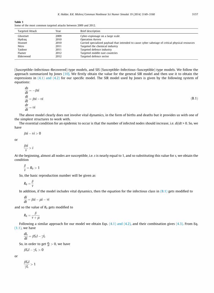
Table 1Some of the most common targeted attacks between 2009 and 2012.

Targeted Attack Year Brief description

Ghostnet 2009 Cyber-espionage on a large scaleHydraq 2010 Operation AuroraStuxnet 2010 Carried specialized payload that intended to cause cyber sabotage of critical physical resourcesNitro 2011 Targeted the chemical industryTaidoor 2011 Targeted defence industryFlamer 2012 Targeted middle east countriesElderwood 2012 Targeted defence sector

K. Haldar, B.K. Mishra / Commun Nonlinear Sci Numer Simulat 19 (2014) 3149–3160 3157

(Susceptible–Infectious–Recovered) type models, and SIS (Susceptible–Infectious–Susceptible) type models. We follow theapproach summarized by Jones [10]. We firstly obtain the value for the general SIR model and then use it to obtain theexpressions in (4.1) and (4.2) for our specific model. The SIR model used by Jones is given by the following system ofequations:

dsdt¼ �bsi

didt¼ bsi� ti

drdt¼ ti

ðB:1Þ

The above model clearly does not involve vital dynamics, in the form of births and deaths but it provides us with one ofthe simplest structures to work with.

The essential condition for an epidemic to occur is that the number of infected nodes should increase, i.e. di/dt > 0. So, wehave

bsi� ti > 0

or

bsim> i

At the beginning, almost all nodes are susceptible, i.e. s is nearly equal to 1, and so substituting this value for s, we obtain thecondition

bm¼ R0 > 1

So, the basic reproduction number will be given as

R0 ¼bm

In addition, if the model includes vital dynamics, then the equation for the infectious class in (B.1) gets modified to

didt¼ bsi� li� mi

and so the value of R0 gets modified to

R0 ¼b

mþ l

Following a similar approach for our model we obtain Eqs. (4.1) and (4.2), and their combination gives (4.3). From Eq.(1.1), we have

dIt

dt¼ bStI � cIt

So, in order to get dItdt > 0, we have

bStI � cIt > 0

or

bStIcIt

> 1

3158 K. Haldar, B.K. Mishra / Commun Nonlinear Sci Numer Simulat 19 (2014) 3149–3160

which is clearly satisfied when

R0t ¼bc> 1 ð4:1Þ

because the attacking population will in general be much more than the fixed target population that we have considered.Similarly from Eq. (1.2), we have

dIdt¼ bSI � ðnþ lÞI

which gives

R0a ¼b

nþ lð4:2Þ

Combining (4.1) and (4.2), we get

R0 ¼

ffiffiffiffiffiffiffiffiffiffiffiffiffiffiffiffiffiffib2

ðnþ lÞc

sð4:3Þ

Appendix C

In this appendix, we briefly outline the geometric approach to global stability problems suggested by Li and Muldowney[11].

Let x#f ðxÞ 2 Rn be a C1 function in an open subset D of Rn. Considering the autonomous dynamical system

x0 ¼ f ðxÞ ðC:1Þ

We assume that the following two hypotheses hold

– (H1) There exists a compact absorbing set K in D.– (H2) Equation (C.1) has a unique equilibrium �x in D.

The method suggests that if an equilibrium point x⁄ is locally stable, then it is also globally stable provided that (H1) and(H2) hold and (B.1) does not have any non-constant periodic solution. It was shown that if (H1) and (H2) hold and (C.1) sat-isfies a Bendixson criteria that is robust under C1 local e-perturbations of f at all non-equilibrium non-wandering points for(C.1), then x⁄ is globally stable in D if it is locally stable. It may be noted that

(1) A function g 2 C1 from D to Rn is called a local perturbation of f at x0 if there exists an open neighborhood of x0 in D, so

that the support supp ðf � gÞ � U and jf � gjC1 < e, where jf � gjC1 ¼ sup jf ðxÞ � gðxÞj þ @f@x ðxÞ �

@g@x ðxÞ

: x 2 Dn o

.

(2) A point x0 2 D is said to be wandering for (B.1) if there exists a neighborhood (say U) of the point x0 and a positive valueT > 0 of time, such that U \ xðt;UÞ ¼ U for all t > T. So, for example, all equilibrium points and limit points will alwaysbe non-wandering.

They introduced a new Bendixson criterion using the Lozinskii measure, which is robust under C1 local perturbations of f.

Taking P(x) to be a n2

�� n

2

�matrix-valued function which is C1 for x 2 D, and defining a quantity

�q2 ¼ lim supt!1

supx02K

1t

Z t

0lðBðxðs; x0ÞÞÞds ðC:2Þ

where B ¼ Pf P�1 þ PJ½2�P�1 and the matrix P is obtained by replacing each of the elements of P by its derivative in the direc-

tion of f. The Lozinskii measure of matrix B with respect to a vector norm in Rn2

� is defined as (as in [14])

lðBÞ ¼ limh!Oþ

jI þ hBj � 1h

ðC:3Þ

The matrix J[2] is the second additive compound matrix of the Jacobian, which for n = 3, is defined as

J½2� ¼j11 þ j22 j23 �j13

j32 j11 þ j33 j12

�j31 j21 j22 þ j33

0B@

1CA ðC:4Þ

Based on these definitions the following theorem was proved by Li and Muldowney [11]:

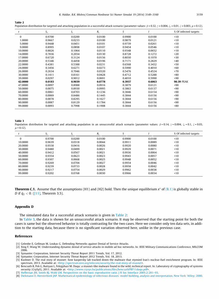
Table 2Population distribution for targeted and attacking population in a successful attack scenario (parameter values: b = 0.32, c = 0.004, nt = 0.01, n = 0.003, l = 0.12).

t St It Rt S I % Of infected targets

0 0.9700 0.0200 0.0100 0.9900 0.0100 <101.0000 0.9667 0.0233 0.0100 0.9879 0.0121 <105.0000 0.9448 0.0451 0.0101 0.9739 0.0261 <109.0000 0.8995 0.0898 0.0107 0.9454 0.0546 <10

10.0000 0.8826 0.1064 0.0110 0.9348 0.0652 >1014.0000 0.7836 0.2034 0.0130 0.8728 0.1272 >2017.0000 0.6720 0.3124 0.0156 0.8030 0.1970 >3020.0000 0.5346 0.4458 0.0196 0.7171 0.2829 >4022.0000 0.4381 0.5388 0.0231 0.6568 0.3432 >5024.0000 0.3456 0.6271 0.0273 0.5990 0.4010 >6026.0000 0.2634 0.7046 0.0320 0.5476 0.4524 >7030.0000 0.1411 0.8161 0.0428 0.4712 0.5288 >8039.0000 0.0297 0.9012 0.0691 0.4010 0.5990 >9042.0000 0.0183 0.9039 0.0778 0.3937 0.6063 90.39 PEAK47.0000 0.0097 0.8988 0.0916 0.3879 0.6121 <9050.0000 0.0075 0.8930 0.0995 0.3863 0.6137 <9060.0000 0.0061 0.8703 0.1236 0.3846 0.6154 <9070.0000 0.0069 0.8486 0.1445 0.3844 0.6156 <9080.0000 0.0078 0.8295 0.1627 0.3844 0.6156 <9090.0000 0.0087 0.8129 0.1784 0.3844 0.6156 <9099.0000 0.0093 0.7998 0.1908 0.3844 0.6156 <80

Table 3Population distribution for targeted and attacking population in an unsuccessful attack scenario (parameter values: b = 0.14, c = 0.004, nt = 0.1, n = 0.03,l = 0.12).

t St It Rt S I % Of infected targets

0 0.9700 0.0200 0.0100 0.9900 0.0100 <1010.0000 0.9639 0.0318 0.0044 0.9911 0.0089 <1020.0000 0.9558 0.0416 0.0026 0.9920 0.0080 <1030.0000 0.9480 0.0499 0.0021 0.9929 0.0071 <1040.0000 0.9412 0.0567 0.0021 0.9936 0.0064 <1050.0000 0.9354 0.0623 0.0023 0.9943 0.0057 <1060.0000 0.9307 0.0668 0.0025 0.9948 0.0052 <1070.0000 0.9269 0.0704 0.0027 0.9954 0.0046 <1080.0000 0.9239 0.0733 0.0028 0.9958 0.0042 <1090.0000 0.9217 0.0754 0.0029 0.9962 0.0038 <1099.0000 0.9202 0.0768 0.0030 0.9966 0.0034 <10

K. Haldar, B.K. Mishra / Commun Nonlinear Sci Numer Simulat 19 (2014) 3149–3160 3159

Theorem C.1. Assume that the assumptions (H1) and (H2) hold. Then the unique equilibrium x⁄ of (B.1) is globally stable inD if �q2 < 0: ([11], Theorem 3.5).

Appendix D

The simulated data for a successful attack scenario is given in Table 2:In Table 3, the data is shown for an unsuccessful attack scenario. It may be observed that the starting point for both the

cases is same but the observed behavior is totally contrasting for the two cases. Here we consider only ten data sets, in addi-tion to the starting data, because there is no significant variation observed here, unlike in the previous case.

References

[1] Gelenbe E, Gellman M, Loukas G. Defending Networks against Denial of Service Attacks.[2] Xing F, Wang W. Understanding dynamic denial of service attacks in mobile ad hoc networks. In: IEEE Military Communications Conference, MILCOM

2006.[3] Symantec Corporation, Internet Security Threat Report 2011 Trends, Vol. 17, 2012.[4] Symantec Corporation, Internet Security Threat Report 2012 Trends, Vol. 18, 2013.[5] Kushner D. The real story of stuxnet: how kaspersky lab tracked down the malware that stymied Iran’s nuclear-fuel enrichment program. In: IEEE

spectrum, 2013. Available at: <http://spectrum.ieee.org/telecom/security/the-real-story-of-stuxnet>.[6] Bencsath B, Pek G, Buttyan L, Felegyhazi M. Duqu: a stuxnet-like malware found in the wild, technical report. In: Laboratory of cryptography of systems

security (CrySyS), 2011. Available at: <http://www.crysys.hu/publications/files/bencsathPBF11duqu.pdf>.[7] Heffernan JM, Smith RJ, Wahl LM. Perspectives on the basic reproductive ratio. J R Soc Interface 2005;2:281–93.[8] Diekmann O, Heesterbeek JAP. Mathematical epidemiology of infectious diseases: model building, analysis and interpretation. New York: Wiley; 2000.

3160 K. Haldar, B.K. Mishra / Commun Nonlinear Sci Numer Simulat 19 (2014) 3149–3160

[9] van den Driessche P, Watmough J. Reproduction numbers and sub-threshold endemic equilibria for compartmental models of disease transmission.Math Biosci 2002;180:29–48.

[10] Jones JH. Notes on R0, Technical Report, Stanford University, 2007. Available at: <https://people.stanford.edu/jhj1/sites/default/files/file/jones-on-r0.pdf>.

[11] Li MY, Muldowney JS. A geometric approach to global-stability problems. SIAM J Math Anal 1996;27(4):1070–83.[12] Li MY, Graef JR, Wang L, Karsai J. Global dynamics of an SEIR model with a varying total population size. Math Biosci 1999;160:191–213.[13] Butler GJ, Waltman P. Persistence in dynamical systems. J Differ Equ 1986;63:225–63.[14] Martin Jr RH. Logarithmic norms and projections applied to linear differential systems. J Math Anal Appl 1974;45.