Fig.1 Solar cell model

Abstract—A scaling fuzzy logic control (FLC) maximum

power point tracking (MPPT) algorithm is suggested in this paper. The scaling FLC algorithm is modified from FLC algorithm to achieve MPPT in spite of single or 10 solar PV cells. Here, our solar system is composed of solar penal, boost dc/dc converter and MPPT controller, and then we use OrCAD Pspice for the system simulation. The simulated cases focus on the steady-state response, the dynamic response to the variation of the solar-cell current or load resistance. The simulated results are illustrated to show the efficacy of the proposed algorithm.

Index Terms—maximum power point tracking (MPPT),

fuzzy logic control (FLC), photovoltaic (PV), boost DC-DC converter.

I. INTRODUCTION In recent years, the petroleum is getting more and more

expensive. The people seek for new green energy, e.g. wind energy, water energy, solar energy, etc… Solar energy is a clean, maintenance-free, and an abundant resource of nature, so it is suitable to be a green energy source. But, there are still some drawbacks as follow: the install cost of solar panels is high, and the conversion efficiency is still lower. The solar system uses the solar module as a source of electrical power supply. Each solar module has an optimal operating point, called the maximum power point (MPP) which changes with its own characteristic as well as cell temperature and sunlight. In other words, the current/voltage curves of photovoltaic (PV) solar-cell module are affected with the sunlight illumination and cell temperature. So, it is not easy to keep the MPP operating when the curve of power versus voltage (P-V) is varying. To overcome this problem, many MPPT algorithms were suggested for tracking the MPP of solar module [1, 4]. Then, one of the well known algorithms for MPPT is Perturb and observe (P&O) algorithm. This P&O algorithm has the advantages of low cost and simple circuit. However, its tracking response is slower because it often results in the swing tracking around the MPP. Thus, perhaps it makes some power loss. Here, a scaling fuzzy logic control algorithm is suggested for MPPT, and modified by fuzzy logic control algorithm [2, 5]. The main goal is to use 25 scaling fuzzy rules and pulse-width-modulation control (PWM) not only for the reduction of the tracking time of

This work was supported in part by the National Science Council of

Taiwan, R.O.C., under Grant NSC 98-2221-E-324-024. Yuen-Haw Chang and Chia-Yu Chang are with the Department and

Graduate Institute of Computer Science and Information Engineering, Chaoyang University of Technology, Taichung County, Taiwan, R.O.C. Post code:413. (e-mail: cyhfyc@cyut.edu.tw, s9727626@cyut.edu.tw).

MPPT, but also for the enhancement of the tracking regulation for the different number of solar cell in parallel [3], sunlight or loading variation. Finally, our overall solar system is designed by combining scaling fuzzy logic, and simulated by using OrCAD Pspice for the cases of steady-state response, dynamic response to the variation of solar-cell current or load (RL). These simulation results are illustrated to show the efficacy of the proposed scheme.

II. MPPT IN STAND-ALONE SOLAR SYSTEMS

A. Solar Cell Model In general, the equivalent models of solar cell have three

types as shown in Fig. 1. Fig. 1(a) shows an ideal model with one current source and diode just. Going a step further, Fig. 1(b) has an extra small resistor to simulate the line loss. And then, Fig. 1(c) has a big internal resistor to realize the solar cell’s power loss. In this paper, we choose the module of Fig. 1(b) for the simulation later.

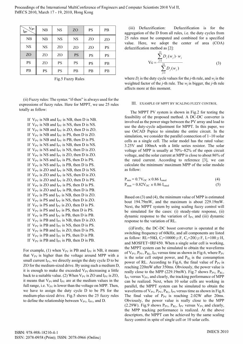
B. MPPT Circuit Frame Fig. 2 shows the overall circuit frame of MPPT PV

system. Our system includes three parts: solar panel, DC-DC converter and MPPT controller. The solar panel we used is a low-power photovoltaic cell with open voltage Voc=3.25V and rated current Irated =100mA. The boost DC-DC converter is adopted in this paper because it is a low-cost and high-efficiency converter. The MPPT controller is shown in the lower half of Fig. 2. According to voltage VPV and current IPV of solar cell in Fig. 2, the duty cycle D will be determined via scaling fuzzy logic and PWM blocks in order to realize MPPT.

C. Solar Cell Characteristic Each solar module has its own characteristic and unique

I-V curve. General speaking, the I-V curve is shown in Fig. 3.

A Maximum Power Point Tracking of PV System by Scaling Fuzzy Control

Yuen-Haw Chang and Chia-Yu Chang

(c) (b) (a)

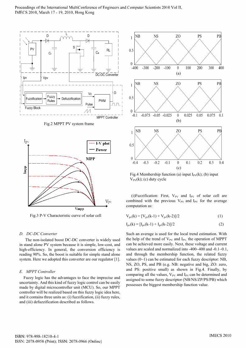
Fig.2 MPPT PV system frame

D. DC-DC Converter The non-isolated boost DC-DC converter is widely used

in stand alone PV system because it is simple, low-cost, and high-efficiency. In general, the conversion efficiency is reading 90%. So, the boost is suitable for simple stand alone system. Here we adopted this converter are our regulator [1].

E. MPPT Controller Fuzzy logic has the advantages to face the imprecise and

uncertainty. And this kind of fuzzy logic control can be easily made by digital microcontroller unit (MCU). So, our MPPT controller will be realized based on this fuzzy logic idea here, and it contains three units as: (i) fuzzification, (ii) fuzzy rules, and (iii) defuzzification described as follows.

(i)Fuzzification: First, VPV and IPV of solar cell are combined with the previous VPV and IPV for the average computation as:

Vpv(k) = [Vpv(k-1) + Vpv(k-2)]/2 (1) Ipv(k) = [Ipv(k-1) + Ipv(k-2)]/2 (2) Such an average is used for the local trend estimation. With the help of the trend of VPV and IPV, the operation of MPPT can be achieved more easily. Next, these voltage and current values are scaled and normalized into -400~400 and -0.1~0.1, and through the membership function, the related fuzzy values (0~1) can be estimated for each fuzzy descriptor: NB, NS, ZO, PS, and PB (e.g. NB: negative and big, ZO: zero, and PS: positive small) as shown in Fig.4. Finally, by comparing all the values, VPV and IPV can be determined and assigned to some fuzzy descriptor (NB/NS/ZP/PS/PB) which possesses the biggest membership function value.

Fig.3 P-V Characteristic curve of solar cell

Fig.4 Membership function (a) input IPV(k); (b) input VPV(k); (c) duty cycle

(a)

(b)

(c)

∑

∑

=

=

⋅= 25

1

25

1

)(

)(Vc

jjj

jj

jj

wD

wwD

(ii) Fuzzy rules: The syntax “if-then” is always used for the expressions of fuzzy rules. Here for MPPT, we use 25 rules totally as follow:

If VPV is NB and IPV is NB, then D is NB. If VPV is NB and IPV is NS, then D is NS. If VPV is NB and IPV is ZO, then D is ZO. If VPV is NB and IPV is PS, then D is ZO.

If VPV is NB and IPV is PB, then D is PS. If VPV is NS and IPV is NB, then D is NS. If VPV is NS and IPV is NS, then D is ZO. If VPV is NS and IPV is ZO, then D is ZO. If VPV is NS and IPV is PS, then D is PS. If VPV is NS and IPV is PB, then D is PS. If VPV is ZO and IPV is NB, then D is NS. If VPV is ZO and IPV is NS, then D is ZO. If VPV is ZO and IPV is ZO, then D is PS. If VPV is ZO and IPV is PS, then D is PS. If VPV is ZO and IPV is PB, then D is PB. If VPV is PS and IPV is NB, then D is ZO. If VPV is PS and IPV is NS, then D is ZO. If VPV is PS and IPV is ZO, then D is PS. If VPV is PS and IPV is PS, then D is PS. If VPV is PS and IPV is PB, then D is PB. If VPV is PB and IPV is NB, then D is ZO. If VPV is PB and IPV is NS, then D is PS. If VPV is PB and IPV is ZO, then D is PS. If VPV is PB and IPV is PS, then D is PB. If VPV is PB and IPV is PB, then D is PB.

For example, (1) when VPV is PB and IPV is NB, it means that VPV is higher than the voltage around MPP with a small current IPV, we directly assign the duty cycle D to be ZO for the medium-sized drive. By using such a medium D, it is enough to make the exceeded VPV decreasing a little back to a suitable value. (2) When VPV is ZO and IPV is ZO, it means that VPV and IPV are at the medium values in the full range, i.e. VPV is lower than the voltage on MPP. Then, we have to assign the duty cycle D to be PS for the medium-plus-sized drive. Fig.5 shows the 25 fuzzy rules to define the relationship between VPV, IPV, and D.

(iii) Defuzzification: Defuzzification is for the

aggregation of the D from all rules, i.e. the duty cycles from 25 rules must be computed and combined for a specified value. Here, we adopt the center of area (COA) defuzzification method as [2]:

(3)

where Dj is the duty cycle values for the j-th rule, and wj is the weighted factor of the j-th rule. The wj is bigger, the j-th rule affects more at this moment.

III. EXAMPLE OF MPPT BY SCALING FUZZY CONTROL

The MPPT PV system is shown in Fig.2 for testing the feasibility of the proposed method. A DC-DC converter is involved as the power stage between the PV array and load to use the duty-cycle adjustment for MPPT. In this paper, we use OrCAD Pspice to simulate the entire circuit. In the simulation, we consider the parallel connection of 1~10 solar cells as a single cell. The solar model has the rated value: 3.25V and 100mA with a little series resistor. The solar voltage of MPP is usually at 70%~82% of the open circuit voltage, and the solar current at MPP is close to about 86% of the rated current. According to reference [3], we can calculate the minimum/ maximum MPP of the solar module as follow: Pmin = 0.7VOC × 0.86 Irated (4) Pman = 0.82VOC × 0.86 Irated (5)

Based on (3) and (4), the minimum value of MPP is estimated bout 194.79mW, and the maximum is about 229.19mW. Next, the MPPT system by using scaling fuzzy control will be simulated for the cases: (i) steady-state response, (ii) dynamic response to the variation of IPV, and (iii) dynamic response to the variation of RL.

(i)Firstly, the DC-DC boost converter is operated at the switching frequency of 60kHz, and all components are listed as follow: RL=50Ω, Ci=10000μF, Co=200μF, L=100μH, and MOSFET=IRF450. When a single solar cell is working, the MPPT system can be simulated to obtain the waveforms of VPV, PPV, PRL, IPV versus time as shown in Fig.6, where PPV is the solar cell output power, and PRL is the consumption power of RL. According to Fig.6, the final value of PPV is reaching 220mW after 350ms. Obviously, the power value is really close to the MPP (229.19mW). Fig.7 shows PPV, PRL, IPV versus VPV, and clearly, the tracking performance of MPP can be realized. Next, when 10 solar cells are working in parallel, the MPPT system can be simulated to obtain the waveforms of VPV, PPV, PRL, IPV versus time as shown in Fig.8. The final value of PPV is reaching 2.02W after 20ms. Obviously, the power value is really close to the MPP (2.29W). Fig.9 shows PPV, PRL, IPV versus VPV, and clearly, the MPP tracking performance is realized. At the above descriptors, the MPPT can be achieved by the same scaling fuzzy control in spite of single cell or 10 solar cells.

Fig.5 Fuzzy Rules

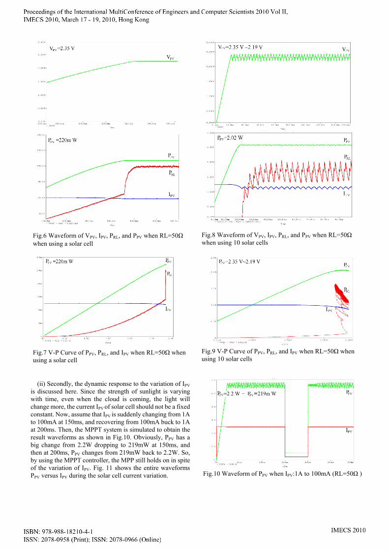
(ii) Secondly, the dynamic response to the variation of IPV is discussed here. Since the strength of sunlight is varying with time, even when the cloud is coming, the light will change more, the current IPV of solar cell should not be a fixed constant. Now, assume that IPV is suddenly changing from 1A to 100mA at 150ms, and recovering from 100mA buck to 1A at 200ms. Then, the MPPT system is simulated to obtain the result waveforms as shown in Fig.10. Obviously, PPV has a big change from 2.2W dropping to 219mW at 150ms, and then at 200ms, PPV changes from 219mW back to 2.2W. So, by using the MPPT controller, the MPP still holds on in spite of the variation of IPV. Fig. 11 shows the entire waveforms PPV versus IPV during the solar cell current variation.

Fig.7 V-P Curve of PPV, PRL, and IPV when RL=50Ω when using a solar cell

Fig.8 Waveform of VPV, IPV, PRL, and PPV when RL=50Ω when using 10 solar cells

Fig.9 V-P Curve of PPV, PRL, and IPV when RL=50Ω when using 10 solar cells

Fig.6 Waveform of VPV, IPV, PRL, and PPV when RL=50Ω when using a solar cell

Fig.10 Waveform of PPV when IPV:1A to 100mA (RL=50Ω )

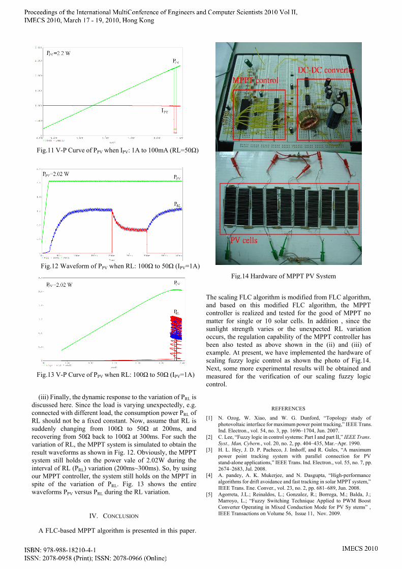
(iii) Finally, the dynamic response to the variation of PRL is discussed here. Since the load is varying unexpectedly, e.g. connected with different load, the consumption power PRL of RL should not be a fixed constant. Now, assume that RL is suddenly changing from 100Ω to 50Ω at 200ms, and recovering from 50Ω back to 100Ω at 300ms. For such the variation of RL, the MPPT system is simulated to obtain the result waveforms as shown in Fig. 12. Obviously, the MPPT system still holds on the power vale of 2.02W during the interval of RL (PRL) variation (200ms~300ms). So, by using our MPPT controller, the system still holds on the MPPT in spite of the variation of PRL. Fig. 13 shows the entire waveforms PPV versus PRL during the RL variation.

IV. CONCLUSION

A FLC-based MPPT algorithm is presented in this paper.

The scaling FLC algorithm is modified from FLC algorithm, and based on this modified FLC algorithm, the MPPT controller is realized and tested for the good of MPPT no matter for single or 10 solar cells. In addition , since the sunlight strength varies or the unexpected RL variation occurs, the regulation capability of the MPPT controller has been also tested as above shown in the (ii) and (iii) of example. At present, we have implemented the hardware of scaling fuzzy logic control as shown the photo of Fig.14. Next, some more experimental results will be obtained and measured for the verification of our scaling fuzzy logic control.

REFERENCES [1] N. Ozog, W. Xiao, and W. G. Dunford, “Topology study of

photovoltaic interface for maximum power point tracking,” IEEE Trans. Ind. Electron., vol. 54, no. 3, pp. 1696–1704, Jun. 2007.

[2] C. Lee, “Fuzzy logic in control systems: Part I and part II,” IEEE Trans. Syst., Man, Cybern., vol. 20, no. 2, pp. 404–435, Mar.–Apr. 1990.

[3] H. L. Hey, J. D. P. Pacheco, J. Imhoff, and R. Gules, “A maximum power point tracking system with parallel connection for PV stand-alone applications,” IEEE Trans. Ind. Electron., vol. 55, no. 7, pp. 2674–2683, Jul. 2008.

[4] A. pandey, A. K. Mukerjee, and N. Dasgupta, “High-performance algorithms for drift avoidance and fast tracking in solar MPPT system,” IEEE Trans. Ene. Conver., vol. 23, no. 2, pp. 681–689, Jun. 2008.

[5] Agorreta, J.L.; Reinaldos, L.; Gonzalez, R.; Borrega, M.; Balda, J.; Marroyo, L.; “Fuzzy Switching Technique Applied to PWM Boost Converter Operating in Mixed Conduction Mode for PV Sy stems” , IEEE Transactions on Volume 56, Issue 11, Nov. 2009.

Fig.11 V-P Curve of PPV when IPV: 1A to 100mA (RL=50Ω)

Fig.12 Waveform of PPV when RL: 100Ω to 50Ω (IPV=1A)

Fig.13 V-P Curve of PPV when RL: 100Ω to 50Ω (IPV=1A)

Fig.14 Hardware of MPPT PV System