Embed Size (px)
Citation preview
Digital Object Identifier (DOI) 10.1007/s002110100258Numer. Math. 89: 457–491 (2001) Numerische
Mathematik
A minimal stabilisation procedurefor mixed finite element methods
F. Brezzi1,2, M. Fortin 3
1 Dipartimento di Matematica, Universita di Pavia, via Ferrata 1, 27100 Pavia, Italy2 Istituto di Analisi Numerica del CNR, via Ferrata 1, 27100 Pavia, Italy3 Departement de Mathematiques et de Statistique, Universite Laval, Quebec G1K7P4,Canada
Received August 9, 1999 / Revised version received May 19, 2000 /Published online March 20, 2001 –c© Springer-Verlag 2001
Summary. Stabilisation methods are often used to circumvent the difficul-ties associated with the stability of mixed finite element methods. Stabili-sation however also means an excessive amount of dissipation or the lossof nice conservation properties. It would thus be desirable to reduce thesedisadvantages to aminimum.Wepresent a general framework, not restrictedto mixed methods, that permits to introduce aminimalstabilising term andhence aminimal perturbation with respect to the original problem. To do so,we rely on the fact thatsome part of the problemis stable and should notbe modified. Sections 2 and 3 present the method in an abstract framework.Section 4 and 5 present two classes of stabilisations for the inf-sup condi-tion in mixed problems. We present many examples, most arising from thediscretisation of flow problems. Section 6 presents examples in which thestabilising terms is introduced to cure coercivity problems.
Mathematics Subject Classification (1991):65N30
1 Introduction
This paper will be devoted primarily to the stabilisation of mixed finiteelementmethods.However,we shall introduceageneral settingwhichmightbe applied to other situations.
Correspondence to: M. Fortin
458 F. Brezzi, M. Fortin
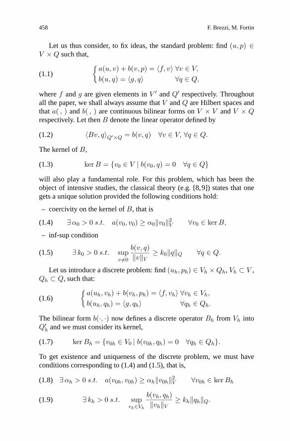
Let us thus consider, to fix ideas, the standard problem: find(u, p) ∈V ×Q such that,
a(u, v) + b(v, p) = 〈f, v〉 ∀v ∈ V,b(u, q) = 〈g, q〉 ∀q ∈ Q,(1.1)
wheref andg are given elements inV ′ andQ′ respectively. Throughoutall the paper, we shall always assume thatV andQ are Hilbert spaces andthata( , ) andb( , ) are continuous bilinear forms onV × V andV × Qrespectively. Let thenB denote the linear operator defined by
〈Bv, q〉Q′×Q = b(v, q) ∀v ∈ V, ∀q ∈ Q.(1.2)
The kernel ofB,
kerB = v0 ∈ V | b(v0, q) = 0 ∀q ∈ Q(1.3)
will also play a fundamental role. For this problem, which has been theobject of intensive studies, the classical theory (e.g. [8,9]) states that onegets a unique solution provided the following conditions hold:
– coercivity on the kernel ofB, that is
∃α0 > 0 s.t. a(v0, v0) ≥ α0‖v0‖2V ∀v0 ∈ kerB,(1.4)
– inf-sup condition
∃ k0 > 0 s.t. supv /=0
b(v, q)‖v‖V ≥ k0‖q‖Q ∀q ∈ Q.(1.5)
Let us introduce a discrete problem: find(uh, ph) ∈ Vh ×Qh, Vh ⊂ V ,Qh ⊂ Q, such that:
a(uh, vh) + b(vh, ph) = 〈f, vh〉 ∀vh ∈ Vh,b(uh, qh) = 〈g, qh〉 ∀qh ∈ Qh.
(1.6)
The bilinear formb(·, ·) now defines a discrete operatorBh from Vh intoQ′h and we must consider its kernel,
kerBh = v0h ∈ V0 | b(v0h, qh) = 0 ∀qh ∈ Qh.(1.7)
To get existence and uniqueness of the discrete problem, we must haveconditions corresponding to (1.4) and (1.5), that is,
∃αh > 0 s.t. a(v0h, v0h) ≥ αh‖v0h‖2V ∀v0h ∈ kerBh(1.8)
∃ kh > 0 s.t. supvh∈Vh
b(vh, qh)‖vh‖V ≥ kh‖qh‖Q.(1.9)
A minimal stabilisation procedure for mixed finite element methods 459
To obtain error estimates, wemust also assume thestability conditions:
αh ≥ α0 > 0.(1.10)
kh ≥ k0 > 0.(1.11)
Problems may arise with both of these conditions. For (1.8) and (1.10)the trouble is thatkerBh is not, in general, a subspace ofkerB, so that (1.8)is not a consequence of (1.4) (unless coercivity hold for the whole spaceV .)
In the same way, an improper choice of the spacesVh andQh can leadto kh vanishing to 0 withh in (1.9). In many instances, conditions (1.10)and (1.11) impose contradictory requirements on the choice of the discretespacesVh andQh, and only quite special choices are admissible.
There are cases where these elaborate constructions are felt as inade-quate. In some situations, for example, it happens that (1.1) is only a part ofa larger problem, for which the choice ofVh andQh is not really free, andwe are led to employ discrete spaces which are not suitable for (1.6).
Stabilisation methods, then, try to recover (1.8)-(1.11) through a modi-fication of the variational formulation. This modification should obviouslypreserve consistency. Ideally, it should be as small as possible, restoringstability without introducing unwanted smoothing properties.
In this paper we shall describe a general framework for the study ofstability issues. We shall also present a general technique that yields manyexamples of stabilised methods which can be analysed in this framework.The basic idea of the technique is that, in several cases, the discretisationat hand has some sort of “partial stability” (to fix ideas, we have a prioribounds for a certainseminormof the solution, but not for the true norm.)Our technique consists then, somehow, in adding theminimummodificationthat allows to restore the full stability.
In the next section, we present and discuss the abstract framework inwhich we are going to set our examples. In Sect. 3 we present, always at theabstract level, a general stabilisation technique, with abstract stability theo-rems and error estimates. A first class of applications, together with severalexamples, will be discussed in Sect. 4, and a second class of applications,with several other examples, will be the object of Sect. 5. Roughly speak-ing, the two classes of applications will correspond to two different waysof stabilising problems of type (1.1) when theinf-supcondition (1.9),(1.11)does not hold: in the first class of stabilisations we assume that we have astability result for a pairVh − Qh, whereQh ⊂ Qh, while in the secondclass we only assume a sort ofweak stabilitythat will be made precise lateron. Applications to problems where the ellipticity in the kernel (1.8), (1.10)is needed are then considered in Sect. 6.
460 F. Brezzi, M. Fortin
Other important general results on stabilisations for this type of problemscan be found in [19,4,5,24] and the references therein. See also [9] foradditional references.
2 An abstract framework
We consider here a very general problem. LetW be a Hilbert space, letAbe inL(W,W ′) (the space of linear continuous operators fromW toW ′,)and letF be inW ′. We want to findX ∈ W such that,
〈AX,Y 〉W ′×W = 〈F, Y 〉W ′×W ∀Y ∈ W.(2.1)
From now on, we shall always assume that
〈AY, Y 〉 ≥ 0 ∀Y ∈ W.(2.2)
The following result is an exercise in functional analysis, but, for theconvenience of the readers, we sketch a proof.
Proposition 2.1. If (2.2) holds, then the two following conditions are equiv-alent:
i) A is an isomorphism fromW ontoW ′.ii) ∃Φ ∈ L(W,W) and a positive real numberαΦ such that
〈AY,Φ(Y )〉W ′×W ≥ αΦ‖Y ‖2W ∀Y ∈ W.(2.3)
Proof of Proposition 2.1.Let J be the Riesz’s operator fromW ′ toW. Theimplication i) =⇒ ii) follows by takingΦ = JA. To prove the converseimplication we denote byId the identity operator inW, and we remark that,if (2.2) holds, then for every positive real numberswe have, for allY ∈ W,
〈(sΦ+ Id)tAY, Y 〉W ′×W = 〈AY, (sΦ+ Id)Y 〉W ′×W ≥ s αΦ‖Y ‖2W .
This easily implies that(sΦ+ Id)tA is an isomorphism fromW ontoW ′.SincesΦ+ Id is an isomorphism fors small enough, theni) follows easily.
Remark 2.1.If (2.2) is not satisfied, we always havei) =⇒ ii) but the con-verse is false. This can be seen by considering inL2(]0,+∞[) the mapping:
(Au)(x) = u(x− 1) for x > 1(Au)(x) = 0 for 0 < x ≤ 1
with Φu := Au. Clearlyii) is satisfied, buti) is not, asA is injective but notsurjective. For an operator that does not satisfy (2.2), we would need two
A minimal stabilisation procedure for mixed finite element methods 461
conditions instead of (2.3), that is:∃Φ1 ∈ L(W,W), Φ2 ∈ L(W,W) suchthat, for allY ∈ W, 〈AY,Φ1(Y )〉W ′×W ≥ α1‖Y ‖2
W ,〈Φ2(Y ), AtY 〉W×W ′ ≥ α2‖Y ‖2
W ,(2.4)
implying thatA is both injective and surjective. Remark 2.2 (stability constant).It must be noted that the “ stability con-stant” of Problem (2.1), that is the smallest constantC such that
‖X‖ ≤ C‖AX‖ ∀X ∈ W,
is not1/αΦ (see (2.3)) but rather‖Φ‖/αΦ. As we are mostly interested in mixed problems, it might be worth show-
ing that this abstract formalism contains the usual theory for Problem (1.1).Indeed, letW = V ×Q,X = (u, p), Y = (v, q), and define 〈AX,Y 〉 = a(u, v) + b(v, p) − b(u, q),
〈F, Y 〉 = 〈f, v〉V ′×V − 〈g, q〉Q′×Q.(2.5)
In this context, it is clear that (2.1) is just another way of writing (1.1). Wesuppose thata(u, u) ≥ 0 for anyu ∈ V , which clearly implies (2.2). Wenow want to get (2.3) from (1.4) and (1.5). We thus consider, for any given(u, p) ∈ V × Q, two auxiliary problems, which have a unique solution if(1.4) and (1.5) hold:
– Find(u1, p1), solution ofa(v, u1) − b(v, p1) = (u, v)V ∀v ∈ V,b(u1, q) = 0 ∀q ∈ Q.(2.6)
– Find(u2, p2), solution ofa(v, u2) − b(v, p2) = 0 ∀v ∈ V,b(u2, q) = (p, q)Q ∀q ∈ Q.(2.7)
We now setΦ(u, p) := (u1 + u2), (p1 + p2) and we have:〈A(X), Φ(X)〉 = a(u, u1 + u2) + b(u1 + u2, p) − b(u, p1 + p2)
= ‖u‖2V + ‖p‖2
Q.(2.8)
Remark 2.3.Problems (2.6) and (2.7) could, by linearity, be combined intoone. We preferred to make more explicit the separate control of‖u‖V and‖p‖Q.
462 F. Brezzi, M. Fortin
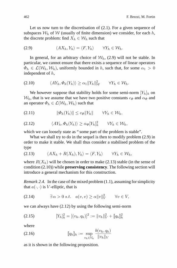
Let us now turn to the discretisation of (2.1). For a given sequence ofsubspacesWh of W (usually of finite dimension) we consider, for eachh,the discrete problem: findXh ∈ Wh such that
〈AXh, Yh〉 = 〈F, Yh〉 ∀Yh ∈ Wh.(2.9)
In general, for an arbitrary choice ofWh, (2.9) will not be stable. Inparticular, we cannot ensure that there exists a sequence of linear operatorsΦh ∈ L(Wh,Wh), uniformly bounded inh, such that, for someα1 > 0independent ofh,
〈AYh, Φh(Yh)〉 ≥ α1‖Yh‖2W ∀Yh ∈ Wh.(2.10)
We however suppose that stability holds for some semi-norm[Yh]h onWh, that is we assume that we have two positive constantscΦ andαΦ andan operatorΦh ∈ L(Wh,Wh) such that
‖Φh(Yh)‖ ≤ cΦ‖Yh‖ ∀Yh ∈ Wh,(2.11)
〈AYh, Φh(Yh)〉 ≥ αΦ[Yh]2h ∀Yh ∈ Wh,(2.12)
which we can loosely state as “ some part of the problem is stable”.What we shall try to do in the sequel is then to modify problem (2.9) in
order to make it stable. We shall thus consider a stabilised problem of thetype
〈AXh +R(Xh), Yh〉 = 〈F, Yh〉 ∀Yh ∈ Wh,(2.13)
whereR(Xh) will be chosen in order to make (2.13) stable (in the sense ofcondition (2.10)) whilepreserving consistency. The following section willintroduce a general mechanism for this construction.
Remark 2.4.In the case of themixed problem (1.1), assuming for simplicitythata(·, ·) is V -elliptic, that is
∃α > 0 s.t. a(v, v) ≥ α‖v‖2V ∀v ∈ V,(2.14)
we can always have (2.12) by using the following semi-norm
[Yh]2h = [(vh, qh)]2 := ‖vh‖2V + [[qh]]2h(2.15)
where
[[qh]]h := supvh∈Vh
b(vh, qh)‖vh‖V(2.16)
as it is shown in the following proposition.
A minimal stabilisation procedure for mixed finite element methods 463
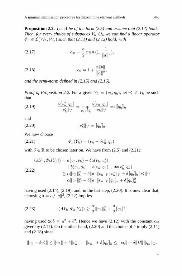
Proposition 2.2. LetA be of the form (2.5) and assume that (2.14) holds.Then, for every choice of subspacesVh, Qh we can find a linear operatorΦh ∈ L(Wh,Wh) such that (2.11) and (2.12) hold, with
αΦ =α
2min (1,
1‖a‖2 ),(2.17)
cΦ = 1 +α‖b‖‖a‖2 ,(2.18)
and the semi-norm defined in (2.15) and (2.16).
Proof of Proposition 2.2.For a givenYh = (vh, qh), let v∗h ∈ Vh be such
thatb(v∗
h, qh)‖v∗h‖V
= supvh∈Vh
b(vh, qh)‖vh‖V =: [[qh]]h(2.19)
and
‖v∗h‖V = [[qh]]h.(2.20)
We now choose
Φh(Yh) = (vh − δv∗h, qh),(2.21)
with δ ∈ R to be chosen later on. We have from (2.5) and (2.21):
〈AYh, Φh(Yh)〉 = a(vh, vh) − δa(vh, v∗h)
+b(vh, qh) − b(vh, qh) + δb(v∗h, qh)
≥ α‖vh‖2V − δ‖a‖‖vh‖V ‖v∗
h‖V + δ[[qh]]h‖v∗h‖V
= α‖vh‖2V − δ‖a‖‖vh‖V [[qh]]h + δ[[qh]]2h
(2.22)
having used (2.14), (2.19), and, in the last step, (2.20). It is now clear that,choosingδ = α/‖a‖2, (2.22) implies
〈AYh, Φh Yh)〉 ≥ α
2‖vh‖2
V +δ
2[[qh]]2h(2.23)
having used2ab ≤ a2 + b2. Hence we have (2.12) with the constantαΦgiven by (2.17). On the other hand, (2.20) and the choice ofδ imply (2.11)and (2.18) since
‖vh − δv∗h‖ ≤ ‖vh‖ + δ‖v∗
h‖ = ‖vh‖ + δ[[qh]]h ≤ ‖vh‖ + δ‖B‖ ‖qh‖Q.
464 F. Brezzi, M. Fortin
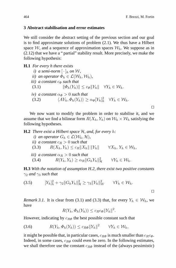
3 Abstract stabilisation and error estimates
We still consider the abstract setting of the previous section and our goalis to find approximate solutions of problem (2.1). We thus have a HilbertspaceW, and a sequence of approximation spacesWh. We suppose as in(2.12) that we have a “ partial” stability result. More precisely, we make thefollowing hypothesis:
H.1 For every h there existsi) a semi-norm[ · ]h onW,
ii) an operatorΦh ∈ L(Wh,Wh),iii) a constantcΦ such that
‖Φh(Yh)‖ ≤ cΦ‖Yh‖ ∀Yh ∈ Wh.(3.1)
iv) a constantαΦ > 0 such that〈AYh, Φh(Yh)〉 ≥ αΦ[Yh]2h ∀Yh ∈ Wh.(3.2)
We now want to modify the problem in order to stabilise it, and we
assume that we find a bilinear formR(Xh, Yh) onWh × Wh satisfying thefollowing hypotheses.
H.2 There exist a Hilbert spaceH, and, for everyh:i) an operatorGh ∈ L(Wh,H),
ii) a constantcR > 0 such thatR(Xh, Yh) ≤ cR‖Xh‖ ‖Yh‖ ∀Xh, Yh ∈ Wh,(3.3)
iii) a constantαR > 0 such thatR(Yh, Yh) ≥ αR‖GhYh‖2
H ∀Yh ∈ Wh.(3.4)
H.3With the notation of assumption H.2, there exist two positive constantsγ2 andγ3 such that
[Yh]2h + γ2‖GhYh‖2H ≥ γ3‖Yh‖2
W ∀Yh ∈ Wh.(3.5)
Remark 3.1.It is clear from (3.1) and (3.3) that, for everyYh ∈ Wh, wehave
R(Yh, Φh(Yh)) ≤ cRcΦ‖Yh‖2.
However, indicating bycRΦ the best possible constant such that
R(Yh, Φh(Yh)) ≤ cRΦ‖Yh‖2 ∀Yh ∈ Wh,(3.6)
it might be possible that, in particular cases,cRΦ is much smaller thancRcΦ.Indeed, in some cases,cRΦ could even be zero. In the following estimates,we shall therefore use the constantcRΦ instead of the (always pessimistic)
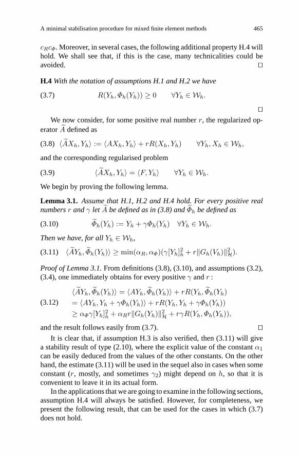
A minimal stabilisation procedure for mixed finite element methods 465
cRcΦ. Moreover, in several cases, the following additional property H.4 willhold. We shall see that, if this is the case, many technicalities could beavoided. H.4With the notation of assumptions H.1 and H.2 we have
R(Yh, Φh(Yh)) ≥ 0 ∀Yh ∈ Wh.(3.7)
We now consider, for some positive real numberr, the regularized op-
eratorA defined as
〈AXh, Yh〉 := 〈AXh, Yh〉 + rR(Xh, Yh) ∀Yh, Xh ∈ Wh,(3.8)
and the corresponding regularised problem
〈AXh, Yh〉 = 〈F, Yh〉 ∀Yh ∈ Wh.(3.9)
We begin by proving the following lemma.
Lemma 3.1. Assume that H.1, H.2 and H.4 hold. For every positive realnumbersr andγ let A be defined as in (3.8) andΦh be defined as
Φh(Yh) := Yh + γΦh(Yh) ∀Yh ∈ Wh.(3.10)
Then we have, for allYh ∈ Wh,
〈AYh, Φh(Yh)〉 ≥ min(αR, αΦ)(γ[Yh]2h + r‖Gh(Vh)‖2H).(3.11)
Proof of Lemma 3.1.From definitions (3.8), (3.10), and assumptions (3.2),(3.4), one immediately obtains for every positiveγ andr :
〈AYh, Φh(Yh)〉 = 〈AYh, Φh(Yh)〉 + rR(Yh, Φh(Yh)= 〈AYh, Yh + γΦh(Yh)〉 + rR(Yh, Yh + γΦh(Yh))≥ αΦγ[Yh]2h + αRr‖Gh(Yh)‖2
H + rγR(Yh, Φh(Yh)),(3.12)
and the result follows easily from (3.7). It is clear that, if assumption H.3 is also verified, then (3.11) will give
a stability result of type (2.10), where the explicit value of the constantα1can be easily deduced from the values of the other constants. On the otherhand, the estimate (3.11) will be used in the sequel also in cases when someconstant (r, mostly, and sometimesγ2) might depend onh, so that it isconvenient to leave it in its actual form.
In the applications thatweare going to examine in the following sections,assumption H.4 will always be satisfied. However, for completeness, wepresent the following result, that can be used for the cases in which (3.7)does not hold.
466 F. Brezzi, M. Fortin
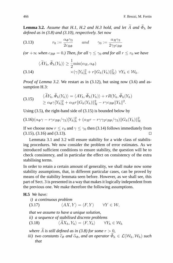
Lemma 3.2. Assume that H.1, H.2 and H.3 hold, and letA and Φh bedefined as in (3.8) and (3.10), respectively. Set now
r0 :=αΦγ3
2cRΦand γ0 :=
αRγ3
2γ2cRΦ(3.13)
(or +∞ whencRΦ = 0.) Then, for allγ ≤ γ0 and for all r ≤ r0 we have
〈AYh, Φh(Yh)〉 ≥ 12min(αR, αΦ)
×(γ[Yh]2h + r‖Gh(Vh)‖2H) ∀Yh ∈ Wh.(3.14)
Proof of Lemma 3.2.We restart as in (3.12), but using now (3.6) and as-sumption H.3:
〈AYh, Φh(Yh)〉 = 〈AYh, Φh(Yh)〉 + rR(Yh, Φh(Yh)≥ αΦγ[Yh]2h + αRr‖Gh(Yh)‖2
H − rγcRΦ‖Yh‖2.(3.15)
Using (3.5), the right-hand side of (3.15) is bounded below by
(αΦγ − rγcRΦ/γ3)[Yh]2h + (αRr − rγγ2cRΦ/γ3)‖Gh(Yh)‖2H(3.16)
If we choose nowr ≤ r0 andγ ≤ γ0 then (3.14) follows immediately from(3.15), (3.16) and (3.13).
Lemmata 3.1 and 3.2 will ensure stability for a wide class of stabilis-ing procedures. We now consider the problem of error estimates. As weintroduced sufficient conditions to ensure stability, the question will be tocheck consistency, and in particular the effect on consistency of the extrastabilising terms.
In order to retain a certain amount of generality, we shall make now somestability assumptions, that, in different particular cases, can be proved bymeans of the stability lemmata seen before. However, as we shall see, thispart of Sect. 3 is presented in a way that makes it logically independent fromthe previous one. We make therefore the following assumptions.
H.5 We have:i) a continuous problem
〈AX,Y 〉 = 〈F, Y 〉 ∀Y ∈ W,(3.17)
that we assume to have a unique solution,ii) a sequence of stabilised discrete problems
〈AXh, Yh〉 = 〈F, Yh〉 ∀Yh ∈ Wh(3.18)
whereA is still defined as in (3.8) for somer > 0,iii) two constantscΦ and αΦ, and an operatorΦh ∈ L(Wh,Wh) such
that
A minimal stabilisation procedure for mixed finite element methods 467
‖Φh(Yh)‖ ≤ cΦ‖Yh‖ ∀Yh ∈ Wh,(3.19)
and〈AYh, Φh(Yh)〉 ≥ αΦ‖Yh‖2 ∀Yh ∈ Wh.(3.20)
We have then the following error bound.
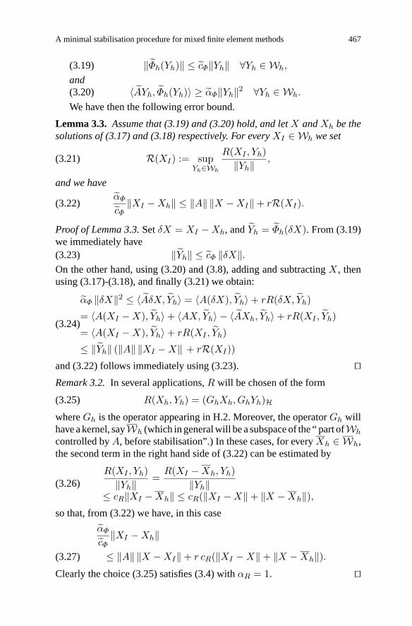
Lemma 3.3. Assume that (3.19) and (3.20) hold, and letX andXh be thesolutions of (3.17) and (3.18) respectively. For everyXI ∈ Wh we set
R(XI) := supYh∈Wh
R(XI , Yh)‖Yh‖ ,(3.21)
and we haveαΦcΦ
‖XI −Xh‖ ≤ ‖A‖ ‖X −XI‖ + rR(XI).(3.22)
Proof of Lemma 3.3.SetδX = XI −Xh, andYh = Φh(δX). From (3.19)we immediately have
‖Yh‖ ≤ cΦ ‖δX‖.(3.23)
On the other hand, using (3.20) and (3.8), adding and subtractingX, thenusing (3.17)-(3.18), and finally (3.21) we obtain:
αΦ ‖δX‖2 ≤ 〈AδX, Yh〉 = 〈A(δX), Yh〉 + rR(δX, Yh)= 〈A(XI −X), Yh〉 + 〈AX, Yh〉 − 〈AXh, Yh〉 + rR(XI , Yh)= 〈A(XI −X), Yh〉 + rR(XI , Yh)≤ ‖Yh‖ (‖A‖ ‖XI −X‖ + rR(XI))
(3.24)
and (3.22) follows immediately using (3.23). Remark 3.2.In several applications,R will be chosen of the form
R(Xh, Yh) = (GhXh, GhYh)H(3.25)
whereGh is the operator appearing in H.2. Moreover, the operatorGh willhaveakernel, sayWh (which ingeneralwill beasubspaceof the “ part ofWh
controlled byA, before stabilisation”.) In these cases, for everyXh ∈ Wh,the second term in the right hand side of (3.22) can be estimated by
R(XI , Yh)‖Yh‖ =
R(XI −Xh, Yh)‖Yh‖
≤ cR‖XI −Xh‖ ≤ cR(‖XI −X‖ + ‖X −Xh‖),(3.26)
so that, from (3.22) we have, in this case
αΦcΦ
‖XI −Xh‖≤ ‖A‖ ‖X −XI‖ + r cR(‖XI −X‖ + ‖X −Xh‖).(3.27)
Clearly the choice (3.25) satisfies (3.4) withαR = 1.
468 F. Brezzi, M. Fortin
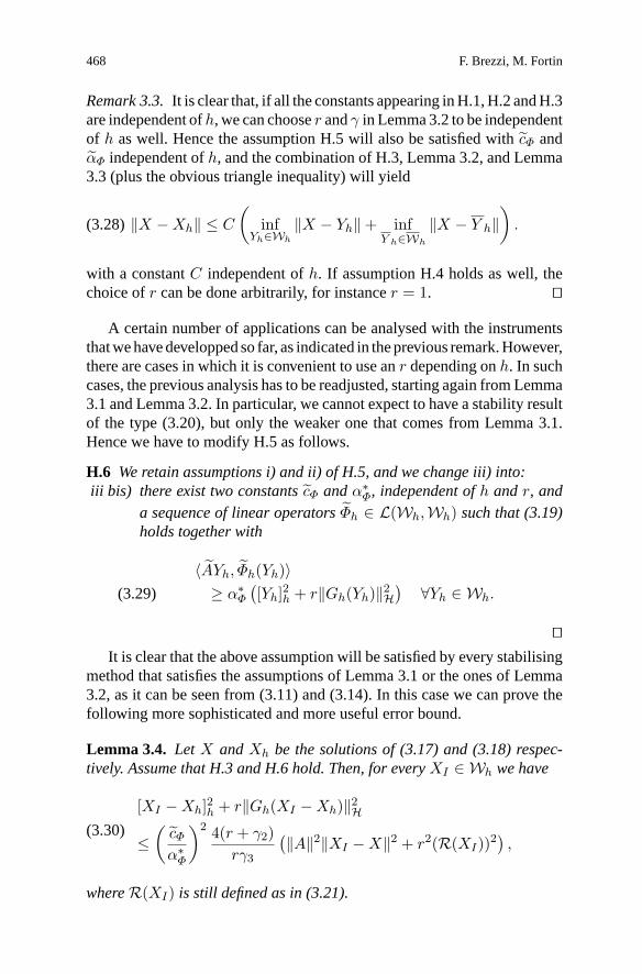
Remark 3.3.It is clear that, if all the constants appearing inH.1,H.2 andH.3are independent ofh, we can chooser andγ in Lemma3.2 to be independentof h as well. Hence the assumption H.5 will also be satisfied withcΦ andαΦ independent ofh, and the combination of H.3, Lemma 3.2, and Lemma3.3 (plus the obvious triangle inequality) will yield
‖X −Xh‖ ≤ C
(inf
Yh∈Wh
‖X − Yh‖ + infY h∈Wh
‖X − Y h‖).(3.28)
with a constantC independent ofh. If assumption H.4 holds as well, thechoice ofr can be done arbitrarily, for instancer = 1.
A certain number of applications can be analysed with the instrumentsthatwehavedeveloppedso far, as indicated in theprevious remark.However,there are cases in which it is convenient to use anr depending onh. In suchcases, the previous analysis has to be readjusted, starting again from Lemma3.1 and Lemma 3.2. In particular, we cannot expect to have a stability resultof the type (3.20), but only the weaker one that comes from Lemma 3.1.Hence we have to modify H.5 as follows.
H.6 We retain assumptions i) and ii) of H.5, and we change iii) into:iii bis) there exist two constantscΦ andα∗
Φ, independent ofh andr, anda sequence of linear operatorsΦh ∈ L(Wh,Wh) such that (3.19)holds together with
〈AYh, Φh(Yh)〉≥ α∗
Φ
([Yh]2h + r‖Gh(Yh)‖2
H) ∀Yh ∈ Wh.(3.29)
It is clear that the above assumption will be satisfied by every stabilising
method that satisfies the assumptions of Lemma 3.1 or the ones of Lemma3.2, as it can be seen from (3.11) and (3.14). In this case we can prove thefollowing more sophisticated and more useful error bound.
Lemma 3.4. LetX andXh be the solutions of (3.17) and (3.18) respec-tively. Assume that H.3 and H.6 hold. Then, for everyXI ∈ Wh we have
[XI −Xh]2h + r‖Gh(XI −Xh)‖2H
≤(cΦα∗Φ
)2 4(r + γ2)rγ3
(‖A‖2‖XI −X‖2 + r2(R(XI))2),
(3.30)
whereR(XI) is still defined as in (3.21).
A minimal stabilisation procedure for mixed finite element methods 469
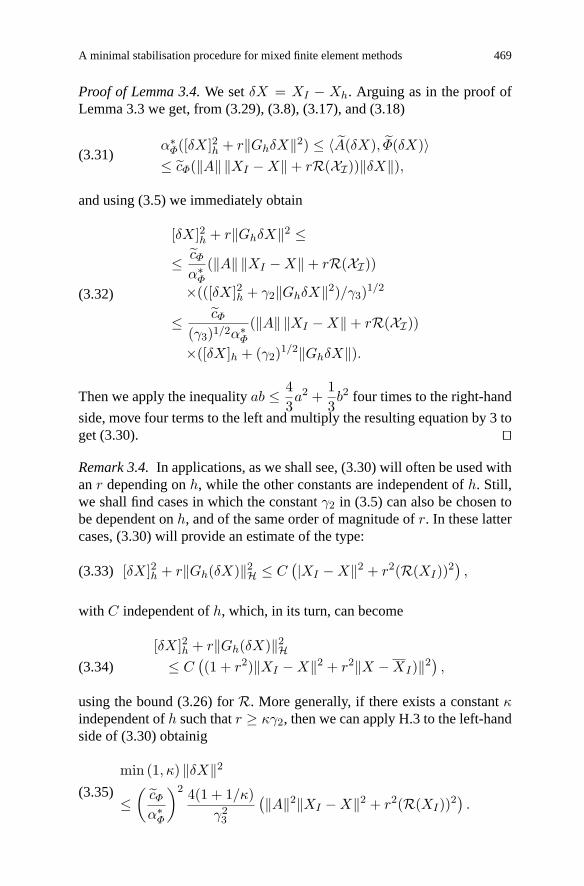
Proof of Lemma 3.4.We setδX = XI − Xh. Arguing as in the proof ofLemma 3.3 we get, from (3.29), (3.8), (3.17), and (3.18)
α∗Φ([δX]2h + r‖GhδX‖2) ≤ 〈A(δX), Φ(δX)〉
≤ cΦ(‖A‖ ‖XI −X‖ + rR(XI))‖δX‖),(3.31)
and using (3.5) we immediately obtain
[δX]2h + r‖GhδX‖2 ≤≤ cΦα∗Φ
(‖A‖ ‖XI −X‖ + rR(XI))
×(([δX]2h + γ2‖GhδX‖2)/γ3)1/2
≤ cΦ(γ3)1/2α∗
Φ
(‖A‖ ‖XI −X‖ + rR(XI))
×([δX]h + (γ2)1/2‖GhδX‖).
(3.32)
Then we apply the inequalityab ≤ 43a2 +
13b2 four times to the right-hand
side, move four terms to the left and multiply the resulting equation by 3 toget (3.30).
Remark 3.4.In applications, as we shall see, (3.30) will often be used withanr depending onh, while the other constants are independent ofh. Still,we shall find cases in which the constantγ2 in (3.5) can also be chosen tobe dependent onh, and of the same order of magnitude ofr. In these lattercases, (3.30) will provide an estimate of the type:
[δX]2h + r‖Gh(δX)‖2H ≤ C
(|XI −X‖2 + r2(R(XI))2),(3.33)
with C independent ofh, which, in its turn, can become
[δX]2h + r‖Gh(δX)‖2H
≤ C((1 + r2)‖XI −X‖2 + r2‖X −XI)‖2) ,(3.34)
using the bound (3.26) forR. More generally, if there exists a constantκindependent ofh such thatr ≥ κγ2, then we can apply H.3 to the left-handside of (3.30) obtainig
min (1, κ) ‖δX‖2
≤(cΦα∗Φ
)2 4(1 + 1/κ)γ2
3
(‖A‖2‖XI −X‖2 + r2(R(XI))2).
(3.35)
470 F. Brezzi, M. Fortin
In other applications,rwill depend onh butγ2 will not. In these cases (3.30)will provide (for r “small”) an estimate of the type
[δX]2h + r‖Gh(δX)‖2H
≤ C
(1r‖XI −X‖2 + r‖X −XI)‖2
),(3.36)
that will then become
[δX]2h + r‖GhδX‖2 ≤ C
(1rhs1 + rhs2
),
by usual interpolation estimates with, in general,s1 ≥ s2 ≥ 0. Then bytakingr = hs we get
[δX]2h + hs‖GhδX‖2 ≤ C
(hs1−s + hs2+s)
with the optimal choice given bys = (s1 − s2)/2.
4 A first class of applications
We shall start by considering a framework which is still abstract but dealswith a subclass of problems (with similar features) containing many of theapplications that will be discussed later on.
Suppose that we are in the context of mixedmethods as in (1.1), and thatwe want to stabilise an inf-sup condition (1.5). Then we have
〈AXh, Yh〉 = a(uh, vh) + b(vh, ph) − b(uh, qh).(4.1)
We want to work on a choice of spacesVh ×Qh for which we do not havestability, and we are aiming at using stabilised problems of the form
a(uh, vh) + b(vh, ph) − b(uh, qh) + rR((uh, ph), (vh, qh))= 〈f, vh〉 − 〈g, qh〉 ∀vh ∈ Vh, ∀qh ∈ Qh.
(4.2)
for a suitable choice ofR. This section will be dedicated to the stabilisationof problems of type (1.1) that satisfy the following assumptions.
A.0 The bilinear formsa( , ) andb( , ) are continuous onV × V andV × Q respectively. Moreovera( , ) is V -elliptic (see (2.14)) andb( , ) satisfies the inf-sup condition (1.5) inV ×Q.
A.1 There exists a subspaceQh ⊂ Qh such that inVh×Qh the problemis stable, that is
∃ k > 0 s.t. supvh∈Vh
b(vh, qh)‖vh‖V ≥ k ‖qh‖Q ∀qh ∈ Qh.(4.3)
A minimal stabilisation procedure for mixed finite element methods 471
We note, incidentally, that theV -ellipticity assumption ona( , ) is notreally relevant and only serves to simplify the presentation. Under the as-sumption A1 it is possible to explicitly buildΦh and a semi-norm[[·]]h toapply our results, as we shall see in the follofing lemma.
Lemma 4.1. Assumptions A.0 and A.1 imply H.1.
Proof of Lemma 4.1.As we have stability inVh×Qh, we can solve, for anyph ∈ Qh, the problem: finduh = uh(ph) ∈ Vh andφh = φh(ph) ∈ Qhsuch that
a(vh, uh) − b(vh, φh) = 0 ∀vh ∈ Vh,b(uh, qh) = (ph, qh)Q = (ph, qh)Q ∀qh ∈ Qh.
(4.4)
whereph = P (ph) = projection ofph ontoQh. We define now
Φh((uh, ph)) := (uh + αuh(ph), ph + αφh(ph))(4.5)
using, for instance, the sameα as in (2.14). From (4.5) and (4.4) we have
a(uh, uh + αuh) + b(uh + αuh, ph) − b(uh, ph + αφh)
= a(uh, uh) + α[a(uh, uh) − b(uh, φh)] + αb(uh, φh))≥ α(‖uh‖2 + ‖ph‖2).
(4.6)
We then have that hypothesis H.1 is satisfied with the choice (4.5) forΦh and the seminorm
[(v, q)]h := ‖v‖2V + ‖Pq‖2
Q.(4.7)
We note in particular that, if A.0 and A.1 hold then the constantscΦ, αΦ
in H.1 will be independent ofh. On the other hand, hypotheses H.2 and H.3will be easily fullfilled, with constants independent ofh, if we take
Gh((vh, qh)) = qh − Pqh(4.8)
with H = Q, and, as in (3.25),
R((uh, ph), (vh, qh)) =(ph − Pph, qh − Pqh
)Q.(4.9)
It is however clear that the class of possible stabilisations is much wider, asshown in the following Lemma.
472 F. Brezzi, M. Fortin
Lemma 4.2. Letsh be a linear operator fromQh into itself, satisfyingsh(qh) = 0 ∀qh ∈ Qh,‖sh(qh)‖2
Q ≥ αS‖qh − Pqh‖2Q ∀qh ∈ Qh,
‖sh(qh)‖Q ≤ cS‖qh‖Q ∀qh ∈ Qh,(4.10)
with constantsαS andcS independent ofh. We take nowH = Q and
Gh((vh, qh)) := sh(qh),(4.11)
R((uh, ph), (vh, qh)) := (sh(ph), sh(qh))Q.(4.12)
If assumptions A.0 and A.1 hold, then H.2 and H.3 will also hold, withconstants independent ofh. Moreover, ifΦh is defined as in (4.5), then H.4will also hold. Finally, H.5 will hold withΦh defined as in Lemma 3.1.
Proof of Lemma 4.2.It is clear that (3.4) follows from (4.12) and (4.11) withαR = 1. It is also clear that (3.3) holds with constantcR = c2S . Similarly(3.5) follows, with constantsγ2 andγ3 independent ofh, from (4.7) and(4.10)-(4.12). Finally, from (4.5) and (4.10)-(4.12) we have
R((vh, qh), Φh(vh, qh)) = (sh(qh), sh(qh + αφh(qh)))Q= ‖sh(qh)‖2
Q + α(s(qh), s(φh(qh)))Q = ‖sh(qh)‖2Q ≥ 0.
(4.13)
The validity of H.5 follows then directly from Lemma 3.1. We can now conclude with a general error estimate for this type of
stabilisations.
Theorem 4.1. Assume that A.0 and A.1 hold, and let(u, p) be the solutionof Problem (1.1). Assume that in (4.2)R is defined through (4.11) and (4.12)using ansh that satisfies (4.10). Then for every positiver Problem (4.2) hasa unique solution(uh, ph), and there exist a consantC, independent ofh,such that, for every(uI , pI) ∈ Vh ×Qh and for everyqh ∈ Qh we have
‖uI − uh‖2V + ‖P (pI − ph)‖2
Q + r‖(Id− P )(pI − ph)‖2Q
≤ C (1 + rr
)(‖u− uI‖2
V + ‖p− pI‖2Q + r2‖pI − qh‖
).
(4.14)
Proof of Theorem 4.1.Under the above assumptions, we can immediatelyapply Lemma 3.4, that in our case gives, for every(uI , pI) ∈ Vh ×Qh,
‖uI − uh‖2V + ‖P (pI − ph)‖2
Q + r‖(Id− P )(pI − ph)‖2Q
≤ C (1 + rr
)(‖u− uI‖2
V + ‖p− pI‖2Q + r2(R((uI , pI))2
)(4.15)
A minimal stabilisation procedure for mixed finite element methods 473
with a constantC independent ofh. Using then (4.10)-(4.12) we have, foreveryqh ∈ Qh
R((uI , pI)) = supqh
(sh(pI), sh(qh))Q‖qh‖Q
= supqh
(sh(pI − qh), sh(qh))Q‖qh‖Q ≤ c2S‖pI − qh‖Q,(4.16)
which inserted in (4.15) gives the result. It is clear that traditional bounds for the error between the continuous so-
lution and the discrete solution can be obtained from (4.14) by a suitable useof the triangle inequality, as we are going to do in the following corollaries.However, as we shall see, it will be convenient to split them in two cases:one in whichr is bounded from below by a positive constant independentof h (but we allow it to be arbitrarily large), and the other in whichr isbounded from above by a positive constant independent ofh (but we allowit to go to zero forh going to zero). In order to simplify the exposition, weintroduce first the following notation: given a Hilbert spaceW , an elementw ∈ W and a subspaceWh ⊂ W we set:
E(w,Wh) := infwh∈Wh
‖w − wh‖W .(4.17)
The following notation will also be convenient: forp ∈ Q, forQh ⊂ Qh ⊂Q and r a positive real number, we set:
(4.18)
Er(p,Qh, Qh) :=(
infqh∈Qh
infqh∈Qh
(‖p− qh‖2Q + r2‖qh − qh‖2
Q
))1/2
.
We have then the following two corollaries, whose proof follows imme-diately from Theorem 4.1.
Corollary 4.1. In the same hypotheses of Theorem 4.1, assume that thereexists anr0 independent ofh such thatr ≥ r0. The there exist a constantC, independent ofr andh, such that
‖u− uh‖2V + ‖p− ph‖2
Q + r‖ph − Pph‖2Q
≤ C (1 + rr
)(E2(u, Vh) + E2
r (p,Qh, Qh)).
(4.19)
Corollary 4.2. In the same hypotheses of Theorem 4.1, assume that thereexists anr0 independent ofh such thatr ≤ r0. The there exist a constantC, independent ofr andh, such that
‖u− uh‖2V + ‖P (p− ph)‖2
Q + r‖(p− ph) − P (p− ph)‖2Q
≤ C (1 + rr
)(E2(u, Vh) + E2
r (p,Qh, Qh)),
(4.20)
474 F. Brezzi, M. Fortin
Remark 4.1.As we have said, the result of Corollary 4.1 applies as well tothe cases in whichr is very large. In these cases, we remark that in (4.18)we can obviously chooseqh ∈ Qh, so thatEr(p,Qh, Qh) ≤ E(p,Qh) andthen from (4.19) we easily obtain
‖u− uh‖2V + ‖p− ph‖2
Q ≤ C((E2(u, Vh) + E2(p,Qh)
),(4.21)
as we could have obtained directly from Lemma 3.3. In fact forr large themethod is equivalent to penalising theunstable partofQh to actually obtaina solution inQh. Thetheoreticalinterest of this choice seems questionable,as we could use directly a discretisation withVh andQh, that would bestable and provide essentially the same error bound. In practice howeverthis choice could still be interesting for various reasons. For instance thechoice ofQh might be dictated by other equations that have to be solvedtoghether with (1.1), or by some optimistic hope of an improvement in theconstants, providing better results for a fixedh.
Remark 4.2.In fact the most interesting case is covered by Corollary 4.2,and corresponds to use anr that goes to zero whenh goes to zero, in thespirit of Remark 3.4. This becomes specially interesting whenE(p,Qh) isof a lower order thanE(u, Vh). In this case, we can add and subtractp inthe expression ofEr(p,Qh, Qh) to obtain
(4.22)
‖p− qh‖2Q + r2‖qh − qh‖2
Q ≤ (1 + 2r2)‖p− qh‖2Q + 2r2‖p− qh‖2
Q
and then (4.20) easily becomes
‖u− uh‖2V + ‖P (p− ph)‖2
Q + r‖(p− ph) − P (p− ph)‖2Q
≤ C
(1r(E2(u, Vh) + E2(p,Qh)) + rE2(p,Qh)
).
(4.23)
WhenQh provides a worse accuracy (with respect toVh andQh,) so that thetermE2(p,Qh) is bigger than the termE2(u, Vh) + E2(p,Qh), a smallrcan, somehow, compensate the difference (see Remark 3.4). Notice that, inthis case, the theory can be applied withQh = 0 (pure penaltymethods.)
Example 4.1 Stabilisation of theQ1 − P0 element
The first case that we consider has been studied by Sylvester [23] forthe Stokes problem. The goal is the stabilisation of the classical bilinear
A minimal stabilisation procedure for mixed finite element methods 475
velocity–constant pressure (Q1–P0) approximation which notoriously suf-fers from stability problems ([21,9,18]). We thus consider the Stokes prob-lem
(4.24)∫Ω ε(u) : ε(v) dx − ∫
Ω p divv dx =∫Ω f · v dx ∀v ∈ (H1
0 (Ω))2∫Ω q divu dx = 0 ∀q ∈ L2
0(Ω),
whereL20(Ω) is the set of square integrable functions with null average.
Let Th be a partition ofΩ into rectangles (we restrict ourselves to thissimplified setting, instead of the general isoparametric case, for the sake ofa lighter presentation.) We now take forVh the space of piecewise bilinearcontinuous functions, and forQh the space of piecewise constants:
(4.25)Vh = vh ∈ (H1
0 (Ω))2 | vh|K = a+ bx+ cy + dxy, ∀K ∈ ThQh = qh ∈ L2
0(Ω) | qh|K = constant, ∀K ∈ Th .
On a rectangular mesh, it is well known that this approximation suffersfrom thecheckerboard spurious modeonph: the kernel of the discrete gra-dient (in the space of piecewise constants) is two-dimensional and containsbesides the expected global constants (which do not belong toQh) a secondmode alternating values in a checkerboard pattern.
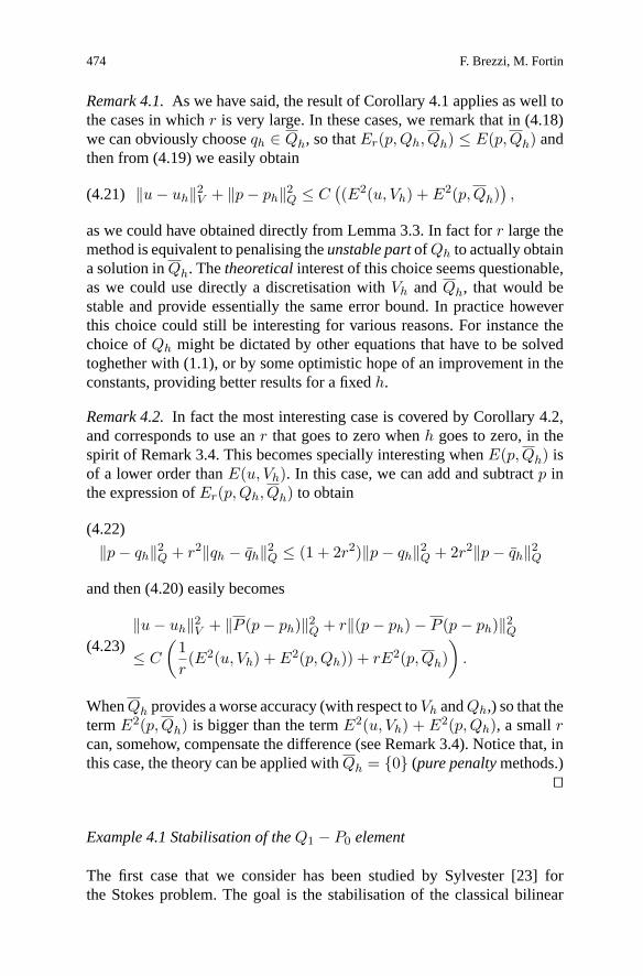
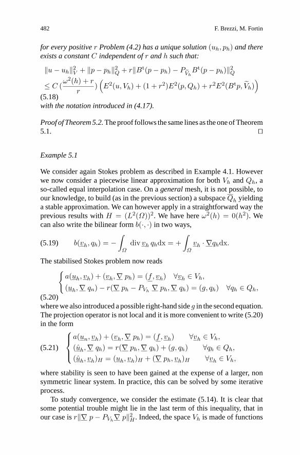
There also exist other unstablemodeswhich emanate from local checker-board patterns ([20]). Indeed, let us splitTh into 2 × 2 macroelements andon a macroelementM
-1
B
-1+1
+1A
D C
Fig. 4.1. Macroelement
476 F. Brezzi, M. Fortin
let us define
CBM =
1 on A,−1 on B,−1 on C,1 on D
(4.26)
andCBh =
qh | qh|M = αCBM ∀M
.(4.27)
It is easily seen (cfr. e.g.[21]) that, definingQ to be the orthogonal com-plement ofCBh inQh, the pairVh×Qh gives a stable approximation whichis equivalent (from the point view of degrees of freedom) to theQ2 − P1piecewise quadratic–piecewise linear approximation. The above theory pro-vides different possibilities for stabilising: we can take
R = R1(ph, qh) =(ph − Pph, qh − Pqh
)(4.28)
which corresponds to (4.9), or set, in each2 × 2 macroelement,sh(qh) =qA + qB − qC − qD, and then use
R = R2(ph, qh) = (sh(ph), sh(qh))(4.29)
which clearly satisfies (4.10). As we have seen in the previous section, bothchoices can be used with arbitrarily larger. It is clear that, forr large,the use of these stabilisations is equivalent to penalising the checkerboardmode and that the result is essentially the same as if one had used the stableapproximationVh ×Qh.
In Sylvester [23], one also uses
R(qh, qh) = ((qB − qA)2 + (qC − qA)2 + (qD − qB)2 + (qD − qC)2) .
For r large, this amounts to take
Qh = qh| qh = constant onM ,that is the space of piecewise constants onmacroelements, which is actuallyan “overstabilisation”.
Remark 4.3.An identical situation is met if we consider a triangular gridTh which has been obtained from a coarser one, sayTh, by splitting as usualeach triangle into four identical ones. Taking the space of piecewise linearcontinuous vectors onTh for velocities and piecewise constants onTh forpressureswe clearly have a stable pair. As above, this can be used to stabiliseaP1−P0 approximation onTh, which by itself would be highly unstable.
A minimal stabilisation procedure for mixed finite element methods 477
Example 4.2 Taylor-Hood approximation for Stokes
Another widely employed approximation for the Stokes problem is the Tay-lor -HoodP2−P1 elementwhichuses, on triangles, a continuousapproxima-tion for pressure of degreeoneand a continuous approximation for velocityof degreetwo. This is apparently a drawback for many users who preferthe simplicity of theP2 − P2 equal-order interpolation. One could eventu-ally think of using stabilisation as follows. Suppose that we use a piecewisequadratic approximation for the pressure.
Let us consider an edge at the interface of two triangles.LetA andB bethe endpoints of this edge andC its midpoint. We can define
sh(qh) = q(A) − 2q(C) + q(B)
andR((vh, qh), (vh, qh)) = Σedges(sh(qh))2 .
Introducing this termwith a larger obviously forcesqh to become linearon the edge, thus reducing the approximation to the Taylor-Hood approxi-mation. It is easily seen that the theory applies and that, forr large, we getthe usualO(h2) error estimates. We could also employ for both variablesa piecewise linear approximation on macro-elements obtained by subdivid-ing each triangle into four subtriangles. One can then use the same trick,forcing the pressure to be linear on each macro-element, obtaining in thelimit the popular variant often called theP1 − isoP2 approximation, withthe usualO(h) error estimate.Wewill not develop further, as this procedure(for obtainingP1− isoP2 as a limit of a penalty method onP1−P1) hasnever been implemented to our knowledge.
Example 4.3 Penalty methods
We still consider the Stokes problem (4.24), and we employ forVh × Qhthe unstable choice,Vh =
vh ∈ (H1
0 (Ω))2 | vh|K ∈ P2(K), ∀K ∈ Th
Qh =qh ∈ L2
0 | qh|K ∈ P1(K), ∀K ∈ Th.
(4.30)
Note that (4.30) is a discontinuous pressure approximation as we imposeno continuity requirement onQh at interfaces.This not a stable choice andthe classical procedures to make it stable are
1. Use a largerVh. The Crouzeix-Raviart element [13] is built along thisoption by adding cubic bubble functions toVh .
478 F. Brezzi, M. Fortin
2. Use a smallerQh. Taking as previouslyQh as the space of piecewiseconstant pressures yields a stable approximation, at the price of a loss ofaccuracy: thisP2 −P0 approximation is onlyO(h) instead of theO(h2)that one expects from the choice ofVh.
Stabilisation opens another avenue. The coupleVh × Qh is stable and wecan define, as in Example 4.1,R(ph, qh) =
(ph − Pph, qh − Pqh
). The
Stokes problem (4.24) becomes
(4.31)∫Ω ε(uh) : ε(vh) dx − ∫
Ω ph divvh dx =∫Ω f · vh dx ∀vh ∈ Vh∫
Ω qh divuh dx + r(ph − Pph, qh − Pqh
)= 0 ∀qh ∈ Qh.
This can also be written, after a few algebraic manipulations, as∫Ω ε(uh) : ε(vh) dx − ∫
Ω ph divvh dx+1r
∫Ω divuhdivvhdx =
∫Ω f · vh dx ∀vh ∈ Vh∫
Ω qh divuh dx = 0 ∀qh ∈ Qh,(4.32)
whereph now lies inQh. This can be read as an augmented Lagrangianformulation for the constraint divuh = 0. It can also be seen that, forr large,(4.32) reduces to the standardP2 −P0 approximation, as the “penalty” term(containig1/r) becomes negligible.
We can now apply the general results. For a fixed value ofr, we get anO(h) convergence rate as the consistency term
R := supqh
R(pI , qh)‖qh‖ = sup
qh
(pI − PpI , qh)‖qh‖
is obviouly onlyO(h). However if we now employ the technique of Remark4.2, takingr = O(h) in (4.23) yields anO(h3/2) estimate for velocities inH1 and for the elementwise mean value of the pressure inL2, as it has beenpointed out in [7].
One can also see that, takingQh = 0, we obtain apure penaltymethod. In this case our analysis provides the following result: if the spaceVh yields anO(hk) approximation, takingr = O(hk/2) we obtain glob-ally anO(hk/2) error estimate on velocities, regardless of the choice ofapproximation forQh.
5 A second class of applications
We consider now another general situation in which our abstract frameworkcan be applied. We go back to a problem of the form (4.1) and we still
A minimal stabilisation procedure for mixed finite element methods 479
make the assumption thata(·, ·) is elliptic onV . On the other hand, insteadof assuming that we know a stable approximationVh × Qh, we make thefollowing hypotheses.
A.2 i) there exists a Hilbert spaceH with V ⊂ H ≡ H ′ ⊂ V ′ and afunctionω : R
+ −→ R+ such that
ω(h)‖vh‖V ≤ ‖vh‖H , ∀vh ∈ Vh.(5.1)
ii) if Bt : Q −→ V ′ is the linear operator associated with the bilinearform b(v, q), we have
Bt(Qh) ⊂ H(5.2)
iii) there exists a linear operatorI from V into Vh and two positiveconstantsσ andcI , independent ofh, such that
(5.3)
‖I(v) − v‖H ≤ σω(h)‖v‖V , and ‖I(v)‖V ≤ cI‖v‖V ∀v ∈ V.
As an example, let us say that this assumption is verified when the pres-sure of Stokes problem is discretised by a space of continuous finite ele-ments. Let us recall that from Proposition 2.2 we have a priori stability inthe semi-norm
[(vh, qh)]2h = ‖vh‖2V + [[qh]]2h(5.4)
with
[[qh]]h := supvh
b(vh, qh)‖vh‖V = sup
vh
(vh, Btqh)H‖vh‖V .(5.5)
We then have that assumption H.1 holds in our case, for the seminorm (5.4),with constants independent ofh. Moreover it is obvious from (5.1) and (5.2)that we have
[[qh]]h ≥ ω(h)‖PVhBtqh‖H(5.6)
wherePVhis the projection operator, inH, ontoVh ⊂ V ⊂ H.
The stability in the semi-norm (5.4) therefore implies also the stabilityin
[(vh, qh)]2∗ = ‖vh‖2 + ω2(h)‖PVhBtqh‖2
H .(5.7)
and H.1 will hold, with constants independent ofh, for the seminorm (5.7)as well. In agreement with the general procedure developed in Sect. 3, wecan now takeH = H with Gh((vh, qh)) = Btqh − PVh
Btqh, and define:
R((uh, ph), (vh, qh)) =(Btph − PVh
Btph, Btqh − PVh
Btqh)H.(5.8)
480 F. Brezzi, M. Fortin
It is clear that H.2 will hold with constants independent ofh. Moreover it iseasy to see, checking the expression ofΦh in (2.21), that it leaves the secondcomponent invariant. Then from (5.8) we easily have that H.4 holds. Weare left with H.3 which will be proved in the next two propositions usingessentially the so-called Verfurth’s trick [25].
Lemma 5.1. Assume that A.0 and A.2 hold. Then
cI [[qh]]h := cI supvh∈Vh
b(vh, qh)‖vh‖V ≥ k0‖q‖Q − cIσω(h)‖Btqh‖H ∀qh ∈ Qh,
(5.9)wherek0 is the inf-sup constant appearing in (1.5),ω(h) is given in (5.1),andσ, cI are given in (5.3).
Proof of Lemma 5.1.We have from the inf-sup condition (1.5), and (5.3)
k0‖qh‖Q ≤ supv
b(v, qh)‖v‖V = sup
v
(b(I(v), qh)
‖v‖V +b(v − I(v), qh)
‖v‖V
)≤ cI sup
v
b(I(v), qh)‖I(v)‖V + sup
v
(v − I(v), Bt(qh))H‖v‖V
≤ cI supvh
b(vh, qh)‖vh‖V + sup
v
‖v − I(v)‖H‖Bt(qh)‖H‖v‖V
≤ cI [[qh]]h + σω(h)‖Btqh‖H ∀qh ∈ Qh.
(5.10)
We can now easily get the following result.
Lemma 5.2. Under the assumptions A.0 and A.2 there exists a constantk,independent ofh, such that
[[qh]]2h + ω2(h)‖Btqh − PVh
Btqh‖2H ≥ k‖qh‖2
Q ∀qh ∈ Qh.(5.11)
Proof of Lemma 5.2.Indeed, from (5.6) one easily obtains
(5.12)
[[qh]]2h + ω2(h)‖Btqh − PVh
Btqh‖2H ≥ ω2(h)‖Btqh‖2
H , ∀qh ∈ Qh,and from (5.9)
2c2I [[qh]]2h ≥ k2
0‖qh‖2Q − 2σ2ω2(h)‖Btqh‖2
H .(5.13)
Then (5.11) is obtained by summing (5.13) and (5.13) with appropriateconstants.
Lemma 5.2 implies that H.3 holds, with the above choices for[ · ]h andGh, with a constantγ3 independent ofh, and withγ2 = ω2(h). In a sense,
A minimal stabilisation procedure for mixed finite element methods 481
we have a stability result that isstrongerthan necessary. However, if we lookat the statement of Lemma 3.4, it is clear that a smallγ2 offers the possibilityof using a smallr without “paying the price”. This is indeed what happensin the following convergence theorem.
Theorem 5.1. Assume that A.2 holds, and let(u, p) be the solution of Prob-lem (1.1). Assume that in (4.2)R is defined through (5.8). Then for everypositiver Problem (4.2) has a unique solution(uh, ph) and there exists aconstantC, independent ofh andr, such that:
(5.14)‖u− uh‖2
V + ‖p− ph‖2Q
≤ C (ω2(h) + r
r)(E2(u, Vh) + (1 + r2)E2(p,Qh) + r2E2(Btp, Vh)
)with the notation introduced in (4.17).
Proof of Theorem 5.1.The proof follows directly from Lemma 3.1, Lemma3.4 the definition ofR given in (5.8) and a few triangle inequalities. In certain cases, as we are going to see in the sequel, it might be moreconvenient to consider another subspaceVh ofH and change the definitionof R (5.8) into
R((uh, ph), (vh, qh)) =(Btph − P
VhBtph, B
tqh − PVhBtqh
)H.(5.15)
This will be allowed, and it will still give optimal error estimates, providedthat we have the following inequality.
A.3 With the notation of aAssumption A.2, there exists a positive constantβ, independent ofh, such that
‖PVhBtqh‖2 + ‖Btqh − P
VhBtqh‖2 ≥ β ‖Btqh‖2 ∀qh ∈ Qh.(5.16)
Indeed, proceeding as in Lemma 5.2, and using (5.6) inequality (5.16)
will imply
[[qh]]2h + ω2(h)‖Btqh − P
VhBtqh‖2
H ≥ k‖qh‖2Q ∀qh ∈ Qh.(5.17)
We summarise the above discussion in the following theorem.
Theorem 5.2. Assume that A.2 and A.3 hold, and let(u, p) be the solutionof Problem (1.1). Assume that in (4.2)R is defined through (5.15). Then
482 F. Brezzi, M. Fortin
for every positiver Problem (4.2) has a unique solution(uh, ph) and thereexists a constantC independent ofr andh such that:
‖u− uh‖2V + ‖p− ph‖2
Q + r‖Bt(p− ph) − PVhBt(p− ph)‖2
Q
≤ C (ω2(h) + r
r)(E2(u, Vh) + (1 + r2)E2(p,Qh) + r2E2(Btp, Vh)
)(5.18)with the notation introduced in (4.17).
Proof of Theorem 5.2.Theproof follows thesame linesas theoneofTheorem5.1.
Example 5.1
We consider again Stokes problem as described in Example 4.1. Howeverwe now consider a piecewise linear approximation for bothVh andQh, aso-called equal interpolation case. On ageneralmesh, it is not possible, toour knowledge, to build (as in the previous section) a subspaceQh yieldinga stable approximation. We can however apply in a straightforward way theprevious results withH = (L2(Ω))2. We have hereω2(h) = 0(h2). Wecan also write the bilinear formb(·, ·) in two ways,
b(vh, qh) = −∫Ω
div vh qhdx = +∫Ωvh · ∇qhdx.(5.19)
The stabilised Stokes problem now readsa(uh, vh) + (vh,∇ ph) = (f, vh) ∀vh ∈ Vh,(uh,∇ qn) − r(∇ ph − PVh
∇ ph,∇ qh) = (g, qh) ∀qh ∈ Qh,(5.20)wherewealso introducedapossible right-hand sideg in the secondequation.The projection operator is not local and it is more convenient to write (5.20)in the form
a(un, vh) + (vh,∇ ph) = (f, vh) ∀vh ∈ Vh,(uh,∇ qh) = r(∇ ph,∇ qh) + (g, qh) ∀qh ∈ Qh,(uh, vh)H = (uh, vh)H + (∇ ph, vh)H ∀vh ∈ Vh,
(5.21)
where stability is seen to have been gained at the expense of a larger, nonsymmetric linear system. In practice, this can be solved by some iterativeprocess.
To study convergence, we consider the estimate (5.14). It is clear thatsome potential trouble might lie in the last term of this inequality, that inour case isr‖∇ p− PVh
∇ p‖2H . Indeed, the spaceVh is made of functions
A minimal stabilisation procedure for mixed finite element methods 483
vanishing on the boundary, while∇ p does not. This induces a bad approx-imation near the boundary and it is easy to see that the term at hand isO(h)for p regular enough. To get the correct order of convergence, we are thusled to user = O(h), which still is going to ensure convergence, as it willgive r ≥ c1ω
2(h) asymptotically.It must be recalled that the more classical stabilised problem (Brezzi-
Pitkaranta[ ])a(uh, vh) + (vh,∇ ph) = (f, vh) ∀vh ∈ Vh,(uh,∇ ph, ) + r(∇ ph,∇ qh) = 0 ∀qh ∈ Qh,
(5.22)
requiresr = 0(h2) in order to get the right order of approximation. This isalso clear from our estimate if we takePVh
≡ 0. At the first sight, onemightthink that stabilising withr = O(h2) is somehow better than usingO(h),as the consistency error becomes smaller. However, numerical experimentsshow that the scheme (5.22) withr = δ h2 suffers from minor instabilities(oscillations of the pressure variable near to the boundary) whenδ is toosmall, while for a largerδ a boundary layer will appear (corresponding toa Neumann boundary conditionr∂p/∂n = 0.) The same is true for thescheme (5.20) if we taker = δ h. On the other hand, very good results havebeen observed experimentally by Habashi et alii [6] if, instead ofPVh
, oneuses the projectionP
Vhon the spaceVh in which boundary conditions are
ignored. In particular, this choice eliminates the boundary layer effect, andallows to take a much biggerr (for instancer = 1) in order to suppress theoscillations. It is clear that with this choice we could recover the right orderof convergence in the right-hand side of (5.14). We are then in the situationof Theorem 5.2, and we have to prove that inequality (5.16) of AssuptionA3 holds. A result of this type is claimed in [12]. Since the proof there israther complicated andmight require someminor fixing, for convenience ofthe reader we report here another proof, limited to the case k=1. The prooffollows, in essence, similar lines (macroelements, continuous dependenceof the constant on the shape of the macroelement and so on) of the originalone in [12], but has a simpler presentation.
Proposition 5.1. LetQh andVh be the space of piecewise linear pressuresand velocities as above, and letVh be the space of piecewise linear contin-uous vectors onTh (without boundary conditions.) There exists a constantβ∗ > 0, independent ofh, such that, for everyqh ∈ Qh and for everywh ∈ Vh, there exists av0
h ∈ Vh verifying
‖v0h‖ ≤ ‖∇qh‖(5.23)
and(v0h,∇qh) + ‖∇qh − wh‖2 ≥ β∗‖∇qh‖2(5.24)
where scalar products and norms are all inL2(Ω).
484 F. Brezzi, M. Fortin
Proof of Proposition 5.1.Let us consider first a macroelementK madeby the collection of triangles having one vertexP of Th in common. Splitqh = q0 + q, whereq0 is such that∇q0 has zero mean value inK andq islinear onK (hence∇q = constant inK.) It is clear that(∇q0,∇q)K = 0.We take nowv0
h, piecewise linear, continuous, vanishing on the boundary ofK and having value
√6∇q at the internal vertexP . An easy computation
shows that:
‖v0h‖0,K = ‖∇q‖0,K(5.25)
and
(v0h,∇q)K =
√23
‖∇q‖20,K .(5.26)
On the other hand,∇q0 belongs to a space (piecewise constant vectors onK, with continuous tangential components, and zero mean onK) whoseintersection with piecewise linear continuous vectors onK is reduced to thezero vector. As we are in finite dimension, there exists a positive constantδK such that, for every∇q0 and for everywh
‖∇q0 − wh‖2 ≥ δK‖∇q0‖20,K .(5.27)
As∇q is clearly continuous and piecewise linear, (5.27) easily implies that‖∇qh − wh‖2 = ‖∇q0 + ∇q − wh‖2
= ‖∇q0 − wh‖2 ≥ δK‖∇q0‖20,K ,
(5.28)
and a simple scaling argument shows immediately thatδK is independentof thesizeofK (notice that (5.28) holdsfor everywh.)
Finally we explicitly point out that
(v0h,∇q0)K =
v0h(P )3
∫K
∇q0dx = 0,(5.29)
whereP is the only vertex internal toK. From (5.26)-(5.29) one then getsthat, for everyqh and for everywh, there is av
0h, piecewise linear, continuous,
and vanishing on the boundary ofK, such that (5.25) holds and
(v0h,∇qh)K + ‖∇qh − wh‖2
0,K ≥ βK‖∇qh‖20,K ,(5.30)
for some positive constantβK independent ofqh andwh. The result (5.23),(5.24) follows then easily from (5.30) by typical instruments (continuity ofβK , splitting ofΩ into macroelements such that each triangle belongs atmost to three different macroelements, and so on.)
With the aid of Proposition 5.1 we can now prove Assumption A.3.
A minimal stabilisation procedure for mixed finite element methods 485
Proposition 5.2. LetQh, Vh and Vh be as in Proposition 5.1. Then thereexists a constantβ > 0 such that
‖PVh∇qh‖2 + ‖∇qh − P
Vh∇qh‖2 ≥ β ‖∇qh‖2 ∀qh ∈ Qh(5.31)
where all the norms are inL2.
Proof of Proposition 5.2.We start by observing that, for everyv0h andqh we
have(v0h,∇qh) = (v0
h, PVh∇qh) ≤ ‖v0
h‖ ‖PVh∇qh‖
≤ β∗
2‖v0h‖2 +
12β∗ ‖PVh
∇qh‖2(5.32)
where the last inequality clearly holds for every positiveβ∗, but we shalluse it for the value ofβ∗ given in (5.24). For everyqh we take nowv0
h asgiven by Proposition 5.1, and using (5.23) we have
(v0h,∇qh) ≤ β∗
2‖∇qh‖2 +
12β∗ ‖PVh
∇qh‖2,(5.33)
that, inserted in (5.24) withwh = PVh
∇qh gives
β∗
2‖∇qh‖2 +
12β∗ ‖PVh
∇qh‖2 +‖∇qh−PVh
∇qh‖2 ≥ β∗ ‖∇qh‖2,(5.34)
and (5.31) follows immediately. Wecan then apply Theorem5.2, and see that, forr = O(1), the stabilised
Stokes problem:
(5.35)a(uh, vh) + (vh,∇ ph) = (f, vh) ∀vh ∈ Vh,(uh,∇ qn) − r(∇ ph − P
Vh∇ ph,∇ qh) = (g, qh) ∀qh ∈ Qh,
is stable andoptimally convergentwhenwe take piecewise linear continuousvelocities and pressure, and forVh the space of piecewise linear continuousvectors without boundary conditions.
Example 5.2
Let us consider a “mixed formulation” of the Dirichet problem.(σ, τ) + (τ ,∇ ψ) = 0 ∀τ ∈ Σ,(τ ,∇ ϕ) = (f, ϕ) ∀ϕ ∈ Ψ,(5.36)
486 F. Brezzi, M. Fortin
having takenΣ = (L2(Ω))2 = H = Σ′, Ψ = H10 (Ω). At the continuous
level, this is nothing but a somewhat bizarre way of writing the standardformulation ∫
Ω∇ ψ · ∇ ϕ dx =
∫Ωf ϕdx ∀ϕ ∈ Ψ.(5.37)
This equivalence however does not hold in general for discretised prob-lems, unlessΨh andΣh are chosen in such a way that the space of gradientsof Ψh is contained inΣh. Let us consider, as an example, a case in whichthis condition is violated: the so-called equal-order interpolation. We take
Ψh = ϕh ∈ H10 (Ω) | ϕh|K ∈ Pk(K)2 ∀K ∈ Th
Σh = τh ∈ (H1(Ω))2 | τh|K ∈ (Pk(K))2 ∀K ∈ Th(5.38)
and we look for (τh, ϕh) in Σh × Ψh such that:(σh, τh) + (τh,∇ ψh) = 0 ∀τh ∈ Σh,(σh,∇ ϕh) = (f, ϕh) ∀ϕh ∈ Ψh.
(5.39)
This is not stable. Indeed one easily checks that we have
supτh
b(τh, ϕh)‖τh‖
=: [[ϕh]]h ≥ ‖PΣh∇ ϕh‖H(5.40)
instead of[[ϕh]]h ≥ ‖∇ ϕh‖H ,(5.41)
which would ensure stability from Poincare’s inequality. Applying our pro-cedure (with, clearly,V = Σ andQ = Ψ ,) we consider the stabilisedproblem,
(5.42)(σh, τh) + (τh,∇ ψh) = 0, ∀τh ∈ Σh(σh,∇ ϕh) + r(∇ ψh − PΣh
∇ ψh,∇ ϕh) = (f, ϕh) ∀ϕh ∈ Ψh.Theorem 5.1 applies directly and we can get a convergence proof to thecorrect order inh. Notice that in this case there are no troubles with theboundary conditions, as we have them onΨ and not onΣ.
Remark 5.1.The stabilised formulation (5.42) can be read as a convex com-bination of the standard discrete formulation∫
Ω∇ ψh · ∇ ϕh dx =
∫Ωf ϕh dx ∀ϕh ∈ Ψh.(5.43)
and the mixed formulation (5.36). IndeedPΣh∇ ψh = σh.
A minimal stabilisation procedure for mixed finite element methods 487
Remark 5.2.Althoughwehave followed the samegeneral framework, thereis a fundamental difference between Example 5.1 and Example 5.2 (besidethe role of boundary conditions.) Indeed in this last case we haveV = Σ =H so that the constantω(h) = 1, while in Example 5.1 we had to employthe equivalence of norms in finite dimensional spaces.
Example 5.3
We discuss now a “viscoelastic ”problem. We consider a variant of Stokesproblem, as a model problem for situations appearing in the finite elementapproximation of some viscoelastic flow problems. This example was, infact, the first instance where the stabilisation technique developed in thispaper was introduced. We refer to [14] and [15] for a more detailed presen-tation.
We takeV = (H10 (Ω))2, Q = L2(Ω) andΣ = (L2(Ω))2s, the space of
symmetric square-integrable tensors, andwe look for(u, p, σ) ∈ V ×Q×Σsuch that:
(σ, τ) + (G(σ), τ) = η (τ , ε(u)) + (F (u), τ) ∀τ ∈ Σ,(div u, q) = 0 ∀q ∈ Q,(σ, ε(v)) + (p, div v) = (f, v) ∀v ∈ V.
(5.44)
Here,η is a constant depending on the viscosity, and the functionsG(·) andF (·) are representing rather complex terms which may vary from a modelto another and can include Lie derivatives in convected models. They canbe left undefined for our present purpose.We now consider the discrete problem,
(5.45)(σh, τh) + (G(σ
h), τ
h) = η (τ
h, ε(uh)) + (F (uh), τh) ∀τ
h∈ Σh,
(div uh, qh) = 0 ∀qh ∈ Qh,(σh, ε(vh)) + (ph, div vh) = (f, vh) ∀vh ∈ Vh,
whereVh,Qh andΣh are finite element subspaces ofV ,Q andΣ, respec-tively. Let us reduce this temporarily to a simple Stokes problem:
(σh, τh) = η (τ
h, ε(uh)) ∀τ
h∈ Σh,
(div uh, qh) = 0 ∀qh ∈ Qh,(σh, ε(vh)) + (ph, div vh) = (f, vh) ∀vh ∈ Vh.
(5.46)
The first equation can now be read as:
σh= PΣh
(ε(uh))(5.47)
488 F. Brezzi, M. Fortin
andwe can understandwhywemay have a stability problem, asPΣh(ε(uh))
is not strong enough to controluh through a Korn’s inequality, unlessΣh isrich enough ([16]). Following the general procedure, we thus write, insteadof (5.45), a stabilised form
(5.48)(σh, τh) + (G(σ
h), τ
h) = η (τ
h, ε(uh)) + (F (uh), τh) ∀τ
h,
(div uh, qh) = 0 ∀qh,(σh, ε(vh)) + r(ε(uh) − PΣh
(ε(uh)), ε(vh))+(ph, div vh) = (f, vh) ∀vh.
Applying the theory is again straightforward. In fact this is very close to theprevious example but is much more relevant in applications, as it stronglywidens the range of possible approximations of (5.44). Indeed, wemay nowuse any reasonable approximation forΣh, the only constraint being to getthe right order of precision. The price to pay is that the projection operatoris most often not local, and that it has to be considered as an extra equationin the problem, which can also be written as
(5.49)(σh, τh) + (G(σ
h), τ
h) = η (τ
h, ε(uh)) + (F (uh), τh) ∀τ
h,
(div uh, qh) = 0 ∀qh,(σh, ε(vh)) + r(ε(uh) − σ
h, ε(vh)) + (ph, div vh) = (f, vh)∀vh,
σh= PΣh
(ε(uh)).
We refer to [14] for details about implementation and numerical results.
6 Coercivity on the kernel ofB
In all previous examples, we have used stabilisation to ensure an inf-supcondition. In many problems, e.g., plate problems, coercivity of the bilinearforma(·, ·) is an equally important issue and we can apply the same generalframework to get stability when needed. Let us then suppose that, in problem(1.1), we have a bilinear form onV ×V that is coercive only onkerB. It isthen natural to suppose that one has
a(v, v) + ‖Bv‖2 ≥ ‖v‖2V ∀v ∈ V.(6.1)
The problem arises because, in general,kerBh is not a subset ofkerB
A minimal stabilisation procedure for mixed finite element methods 489
Let us introduce then, instead of (1.6), a stabilised discrete problem: find(uh, ph) ∈ Vh ×Qh, Vh ⊂ V ,Qh ⊂ Q, such that,a(uh, vh) + b(vh, ph) + r(Buh −Bhuh, Bvh)Q = (f, vh) ∀vh ∈ Vh,b(uh, qh) = (g, qh) ∀qh ∈ Qh.
(6.2)
It is then obvious that we now have coercivity on the kernel ofBh. Hereagain we have employed the strategy of adding the minimum amount ofstabilisation. In fact the stabilising term vanishes ifkerBh ⊂ kerB. Wealso notice that the stabilising term is in fact symmetric, asBhvh is theprojection ofBvh onQh. As to error estimation, it is easy to obtain, usingLemma 3.3, the following result.
Proposition 6.1. Let(u, p) be the solution of (1.6) and(uh, ph) the solutionof the stabilised problem (6.2), with anr independent ofh. Then there existsa constantC, independent ofh, such that:
(6.3)
‖uh − u‖2V + ‖ph − p‖2
Q ≤ C(E2(u, Vh) + E2(p,Qh) + E2(Bu,Qh)
)always with the notation (4.17).
Tofix ideas, let us consider a simplemixed formulation for theDirichlet’sproblem: findu ∈ V = H(div,Ω) andp ∈ Q = L2(Ω) solution of
(u, v) + (p, div v) = 0, ∀v ∈ V(div u, q) = (g, q) ∀q ∈ Q.(6.4)
Here we haveB = div and this is a simple example in which the bilinearform a(·, ·) is coercive only on
kerB = v0 | v0 ∈ H(div,Ω), div v0 = 0 .Except for very special constructions (see e.g. [9] and the references therein)of the spacesVh andQh, the discrete kernelkerBh = kerPQh
div is not asubset ofkerB. This is is the case, for instance, if one uses theMini elementof [3] to build Vh andQh. Let us recall it briefly: letTh be a triangulationof Ω and let, for everyK ∈ Th, bK be the cubic bubble inK defined bybK = λ1λ2λ3. We set:
(6.5)Vh =vh | vh ∈ C0(Ω), vh|K ∈ (P1(K) + αKbK)2 ∀K ∈ Th
Qh =
qh | qh ∈ C0(Ω), qh|K ∈ P1(K) ∀K ∈ Th
.
490 F. Brezzi, M. Fortin
It is classical that this approximation satisfies an inf-sup condition (in facta stronger one than what we need here.)
To get a stabilised problem, we write
(6.6)(uh, vh) + (ph, div vh) + r(divuh − PQh
divuh, divvh) = 0 ∀vh(div uh, qh) = (g, qh) ∀qh.
The projection operator is not, in general, local, and must be considered atthe expenses of an extra equation. However it is easy to see that our generaltheory applies, and that the error estimate (6.3) yields the right order for thespaces at hand. In the particular case above, we can eliminatePQh
divuh asthe second equation of (6.6) states in fact thatPQh
divuh = PQhg. We can
thus replace (6.6) by:
(6.7)(uh, vh) + (ph, div vh) + r(divuh − PQh
g, divvH) = 0 ∀vh ∈ Vh(div uh, qh) = (g, qh) ∀qh ∈ Qh
This is very similar to the satbilisation introduced in [10].This way of modifying the equations to bypass the coercivity problem
proved to be fruitful also in the context of the approximation of Mindlin–Reissner plates ([1]) and shell problems ([22,2]).
7 Conclusions
The various examples presented clearly show that the abstract theory de-veloped here provides a unified framework for a wide class of applications,establishing links between apparently unrelated techniques. The theory alsoprovides a general way of choosing the value of the stabilising parameterwith respect to the mesh size and permits to obtain in some cases sharpererror bounds.
References
1. Arnold D.N., Brezzi F. (1993): Some new elements for the Reissner-Mindlin platemodel, Boundary Value Problems for Partial Differential Equations and Applications(C.Baiocchi and J.-L.Lions eds), Masson, Paris, pp 287–292
2. Arnold D.N., Brezzi F. (1997): Locking-free finite element for shells. Math. Comput.66, 1–14
3. Arnold D.N., Brezzi F., Fortin M. (1984): A stable finite element for the Stokes equa-tions Calcolo21, 337–344
4. Baiocchi C., Brezzi F. (1993): Stabilisation of unstable methods Problemi Attualidell’Analisi e della Fisica Matematica, (P.E. Ricci ed.) Universita La Sapienza, Roma,pp. 59–64
A minimal stabilisation procedure for mixed finite element methods 491
5. Baiocchi C., Brezzi F., Marini D. (1992): Stabilisation of Galerkin methods and appli-cations to domain decomposition. Future Tendencies inComputer Science, Control andApplied Mathematics (A. Bensoussan and J.-P. Verjus eds.), Springer Verlag, Berlin,Lecture Notes in Computer Science653, pp. 345–355
6. G.S. Baruzzi, W.G. Habashi, G. Guevremont, M.M. Hafez (1995): A Second OrderFinite Element Method for the Solution of the Transonic Euler and Navier-StokesEquations. Special issue of the Int. J. Numerical Methods Fluids20, 671–693
7. Boffi D., Lovadina C. (1997): Analysis of a new augmented Lagrangian formulationfor mixed finite element schemes. Numer. Math.75, 405–415
8. Brezzi F. (1974): On the existence, uniqueness and approximation of saddle-pointproblems arising from Lagrangian multipliers. R.A.I.R.O. R-28, 129–151
9. Brezzi F., Fortin M. (1991): Mixed and Hybrid Finite Element Methods, SpringerVerlag, New York, Springer Series in Computatinal Mathematics15,
10. Brezzi F. , Fortin M., Marini D. (1992): Mixed finite element methods with continuousstresses Math. Mod. & Meth. Appl. Sci.3, 257–287
11. Brezzi F., Pitkaranta J. (1984): On the stabilisation of finite element approximations ofthe Stokes equations Efficient solutions of Elliptic Systems (W. Hackbush ed.) Vieweg,pp. 11–19
12. Codina R., Blasco J. (1997): A finite element formulation for the Stokes problemallowing equal velocity-pressure interpolation. Comp. Methods Appl. Mech. Eng.143,373–391
13. Crouzeix M., Raviart P.-A. (1973): Conforming and nonconforming finite elementmethods for solving the stationary Stokes equations R.A.I.R.O. Anal. Numer.7, 33–76
14. Fortin M., Guenette R. (1995): A new mixed finite element method for computingviscoelastic flows. Journal Non Newtonian Fluid Mechanics,60, 27–52
15. Fortin M., Gu’enette R., Pierre R. (1997): Numerical Analysis of the modified EVSSmethod. Comp. Meth. Appl. Mech. Eng.143, 79–95
16. Fortin M., Pierre M. (1989): On the Convergence of the Mixed Method of Marchal andCrochet for Viscoelastic Flows. Comp. Meth. Appl. Mech. Eng.73, 331–340
17. Girault V., Raviart P.-A. (1986): Finite Element Methods for Navier-Stokes Equations,Theory and Algorithms. Springer Verlag, Berlin
18. Gresho P.M., Sani R. (1998): Incompressible Flow and the Finite Element Method, J.Wiley and Sons
19. Hughes T.J.R., Franca L. (1987): A new finite element formulation for computationalfluid dynamics: VII. TheStokes problemwith variouswell-posed boundary conditions:Symmetric formulations that converge for all velocity-pressure spaces. Comp.MethodsAppl. Mech. Eng.65, 85–96
20. Malkus D.S., Hughes T.J.R. (1978): Mixed finite element methods. Reduced and se-lective integration techniques; a unification of concepts. Comp. Methods Appl. Mech.Eng.15, 63–81
21. JohnsonC., Pitkaranta J. (1982): Analysis of somemixed finite elementmethods relatedto reduced integration. Math. Comput.38, 375–400
22. Pitkaranta J. (1995): The problem of membrane locking in finite element analysis ofcylindrical shells. Numer. Math.13, 172–191
23. Sylvester D. (1998): Stabilisation, Sect. 3.13.3 in Incompressible Flow and the FiniteElement Method, P.M. Gresho and R.L. Sani, John Wiley, Chichester
24. Verfurth R. (1995): The stability of finite element methods Numer. Methhods PartialDiffer. Equations11, 93–109
25. Verfurth R. (1984): Error estimates for a mixed finite element approximation of theStokes equation R.A.I.R.O. Anal. Numer.18, 175–182
![Finite fields. Outline [1] Fields [2] Polynomial rings [3] Structure of finite fields [4] Minimal polynomials](https://img.pdfslide.net/doc/110x75/56649d775503460f94a59ac7/finite-fields-outline-1-fields-2-polynomial-rings-3-structure-of-finite.jpg)


![Complete Embedded Minimal Surfaces of Finite …arXiv:math/9508213v1 [math.DG] 9 Aug 1995 Complete Embedded Minimal Surfaces of Finite Total Curvature David Hoffman∗ MSRI 1000 Centennial](https://img.pdfslide.net/doc/110x75/5e3d60412c5aab7cd60ded32/complete-embedded-minimal-surfaces-of-finite-arxivmath9508213v1-mathdg-9-aug.jpg)