A Model for Optimizing Electronic Toll Collection Systems · PDF fileDeploying Electronic Tolls 2 Introduction Newly deployed electronic toll collection (ETC) systems enable bridge,

Deploying Electronic Tolls

1

A Model for Optimizing Electronic Toll CollectionSystems

by David Levinson and Elva Chang

Corresponding Author:David LevinsonAssistant ProfessorDepartment of Civil EngineeringUniversity of Minnesota500 Pillsbury Drive SEMinneapolis, MN 55455

[email protected]

DRAFT August 15, 2001

AbstractThis paper examines the deployment of electronic toll collection (ETC) and develops amodel to maximize social welfare associated with a toll plaza. A payment choice modelestimates the share of traffic using ETC as a function of delay, price, and a fixed cost ofacquiring the in-vehicle transponder. Delay in turn depends on the relative number ofETC and Manual Collection Lanes. Price depends on the discount given to users of theETC Lanes. The fixed cost of acquiring the transponder (not simply a monetary cost, butalso the effort involved in signing up for the program) is a key factor in the model. Oncea traveler acquires the transponder, the cost of choosing ETC in the future declinessignificantly. Welfare depends on the market share of ETC, and includes delay andgasoline consumption, toll collection costs, and social costs such as air pollution. Thiswork examines the best combination of ETC Lanes and toll discount to maximize welfare.Too many ETC lanes cause excessive delay to non-equipped users. Too high a discountcosts the highway agency revenue needed to operate the facility. The model is applied toCalifornia’s Carquinez Bridge, and recommendations are made concerning the numberof dedicated ETC lanes and the appropriate ETC discount


2

Introduction

Newly deployed electronic toll collection (ETC) systems enable bridge, tunnel, and

turnpike operators to save on staffing costs while reducing delay for travelers. Such

systems are not deployed instantaneously. Agencies need to familiarize themselves with

the technology, while distrust and procrastination cause many users to defer expending

time or resources to acquire transponders and establish accounts. To overcome the buy-

in hurdle, some fraction of the cost savings could be returned as a discount for ETC users

to optimize the use of the lanes, leaving everyone better off. The Golden Gate Bridge in

California chose this strategy initially (Fimrite 2001). Alternatively, the buy-in hurdle

could be reduced. For instance, the Japanese Transport Ministry announced a 20%

discount on in-vehicle equipment (which had cost 50,000 yen plus 7,000 yen

installation), since only 12,000 devices had been sold despite the availability of ETC at

63 tollbooths (Asahi Shimbun 2001). Moreover, in the absence of automatic vehicle

identification, people without transponders must be accommodated by manual lanes.

The intent of this paper is to inform decisions that tolling agencies must make

regarding toll discounts, transponder availability and ETC lane dedication. This paper

therefore tackles the question of how quickly lanes should be converted to ETC and what

discount for using ETC would be socially optimal, and extends previous research on ETC

(Al Deek et al 1996, Al Deek et al 1997, Burris and Hildebrand 1996, Friedman and

Waldfogel 1995, Hensher 1991, Lin and Su 1994, Robinson and Van Aerde 1995, Sisson

1995, Woo and Hoel 1991, Zarillo et al 1997).


3

However asking such questions is much easier than answering them. Ideally the

models developed must dynamically optimize over a flexible choice set. For instance,

one would like to determine what share of the initial reluctance to switch to electronic

tolls is fixed with the individual, based on measurable socio-economic, demographic, and

geographic factors, what share depends on exposure, and what share is simply random.

An agency’s decision to deploy ETC lanes in one year will inevitably shape the market

environment it faces in the next.

This paper begins by discussing a dynamic payment choice model that predicts

the users' choice between manual and electronic tolls. Societal benefits and costs and

user payment choices, which vary with demand and the number of ETC lanes, are needed

to determine the best combination in the optimization exercise. The welfare

maximization model is applied to the Carquinez Bridge case. A series of sensitivity

analyses, varying the key model parameters, are performed. Finally, some conclusions

are drawn about the pace of deploying electronic toll collection.

Dynamic Payment Choice Model

The dynamic payment choice model aims to explain the share of manual and

electronic payment in any given year. In this model, the travel time, lane configuration,

discount, and payment choice decision are all interdependent. This model considers the

decisions of drivers (who must choose whether to equip their vehicle with ETC) during

peak periods, including both regular and occasional users, though passenger value of time

is considered in the benefits calculation. Details on the benefit-cost analysis and key

assumptions are given in the appendix.


4

Payment Choice

It is hypothesized that the choice between manual or electronic payment by

drivers depends on the out-of-pocket cost of each alternative and the time associated with

each alternative. The choice also depends on a one-time fixed cost associated with

electronic toll collection, frequency of use of the facility, convenience associated with

avoiding cash or tickets, and the convenience with which the toll agency makes available

transponders. Because there is no data available for these other factors, they are

embedded in an ETC-specific constant. Initially, this constant is expected to have a

negative sign since travelers must obtain transponders and open an ETC account.

Sensitivity tests examine alternative constants. The logit functional form was chosen for

its simplicity of application rather than because of its error distribution (Train 1986). The

linear utility function implies substitutability between the travel time and out-of-pocket

costs. The model posits that individuals using manual payment re-evaluate their payment

mechanism each time there is a change in circumstances (in this case traffic growth, a

change in the lane configuration, and/or discount policy), assumed to be once per year. A

more frequent cycle of user re-evaluation would entail a change in the model because of

the irreversibility assumption described below.

This model estimates payment choice among those who are presently users of

manual lanes. In this model, there is an irreversibility assumption, that an individual who

has chosen ETC stays with electronic payment. However, a certain fraction of electronic

payment users are lost each year because of changing commute patterns associated with

retirement, moving or changing jobs. The fraction of those who stay with the same

commute from year to year is dubbed the “survival rate” (R). This value is taken to be


5

84% based on previous research evaluating the survival of commutes between the same

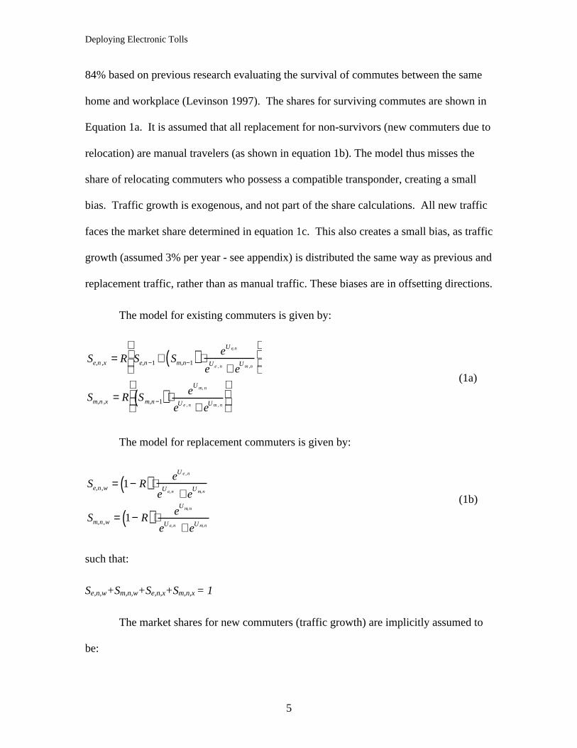
home and workplace (Levinson 1997). The shares for surviving commutes are shown in

Equation 1a. It is assumed that all replacement for non-survivors (new commuters due to

relocation) are manual travelers (as shown in equation 1b). The model thus misses the

share of relocating commuters who possess a compatible transponder, creating a small

bias. Traffic growth is exogenous, and not part of the share calculations. All new traffic

faces the market share determined in equation 1c. This also creates a small bias, as traffic

growth (assumed 3% per year - see appendix) is distributed the same way as previous and

replacement traffic, rather than as manual traffic. These biases are in offsetting directions.

The model for existing commuters is given by:

Se,n ,x = R Se,n −1 + Sm,n−1( ) ⋅eU e, n

eU e , n + e

U m ,n

Sm,n ,x = R Sm,n −1( )⋅ eU m, n

eU e , n + eU m , n

(1a)

The model for replacement commuters is given by:

Se,n,w = 1− R( )⋅eU e , n

eU e, n + e

U m, n

Sm,n,w = 1− R( )⋅ eU m, n

eU e, n + eU m, n

(1b)

such that:

Se,n,w+Sm,n,w+Se,n,x+Sm,n,x = 1

The market shares for new commuters (traffic growth) are implicitly assumed to

be:


6

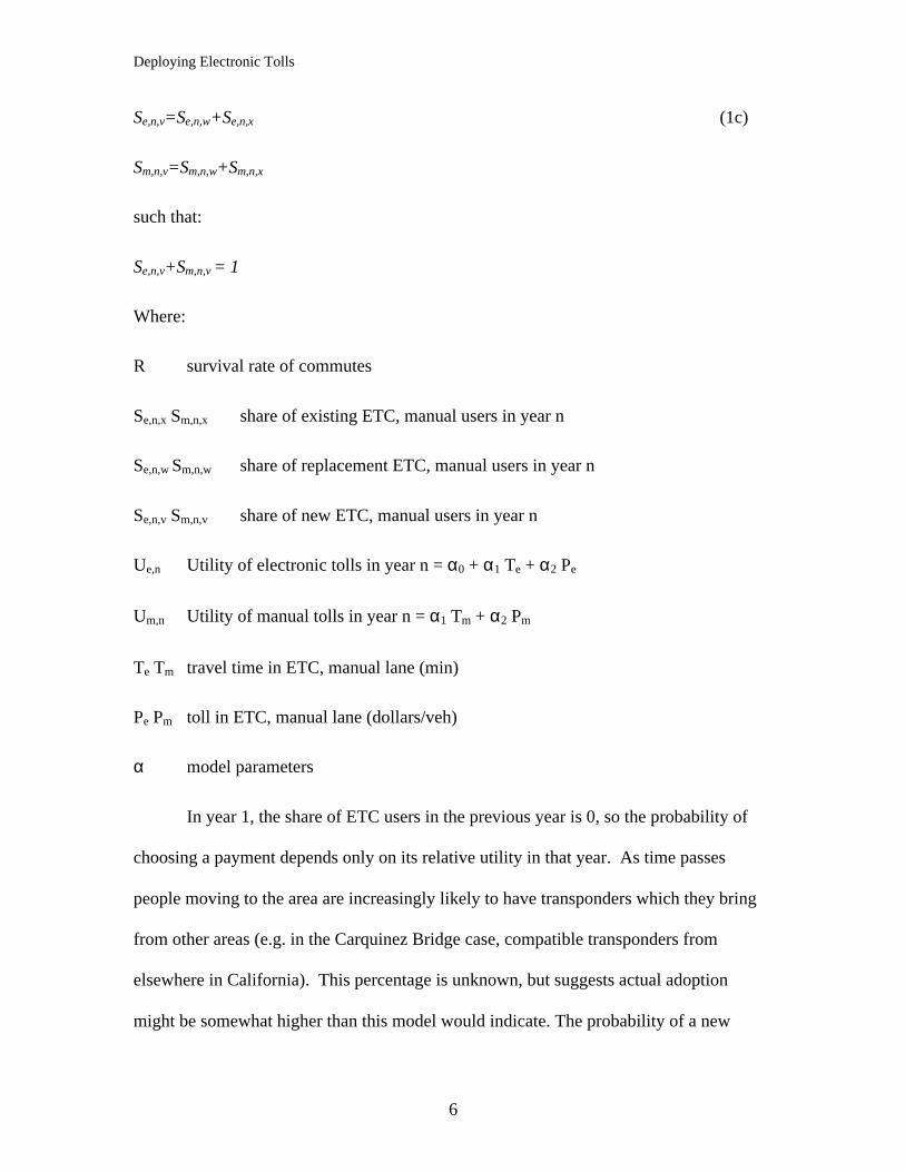
Se,n,v=Se,n,w+Se,n,x (1c)

Sm,n,v=Sm,n,w+Sm,n,x

such that:

Se,n,v+Sm,n,v = 1

Where:

R survival rate of commutes

Se,n,x Sm,n,x share of existing ETC, manual users in year n

Se,n,w Sm,n,w share of replacement ETC, manual users in year n

Se,n,v Sm,n,v share of new ETC, manual users in year n

Ue,n Utility of electronic tolls in year n = α0 + α1 Te + α2 Pe

Um,n Utility of manual tolls in year n = α1 Tm + α2 Pm

Te Tm travel time in ETC, manual lane (min)

Pe Pm toll in ETC, manual lane (dollars/veh)

α model parameters

In year 1, the share of ETC users in the previous year is 0, so the probability of

choosing a payment depends only on its relative utility in that year. As time passes

people moving to the area are increasingly likely to have transponders which they bring

from other areas (e.g. in the Carquinez Bridge case, compatible transponders from

elsewhere in California). This percentage is unknown, but suggests actual adoption

might be somewhat higher than this model would indicate. The probability of a new


7

bridge user choosing electronic tolls in a given year depends on the utilities that the user

faces in that year, which may differ from those users faced in previous (or will face in

future) years. The model is solved for a representative traveler at the expected value of

delay and the given discount and ETC-specific constant.

The baseline scenario coefficient on time was borrowed from previous studies on

the sensitivity of choice to travel time (α1 = -0.03) (Ben-Akiva and Lerman 1985). The

logit scale parameter GEV is assumed to equal 1 (Train 1986). From this and the

assumed weighted value of time (VT) of $17.41 per vehicle-hour (Gillen et al. 1999), the

coefficient on price is estimated. Using base-year data and these values, an alternative-

specific constant ( 0) is computed. To test the model, a sensitivity analysis of various

parameters was conducted; this is discussed in a later section. Model predictions are

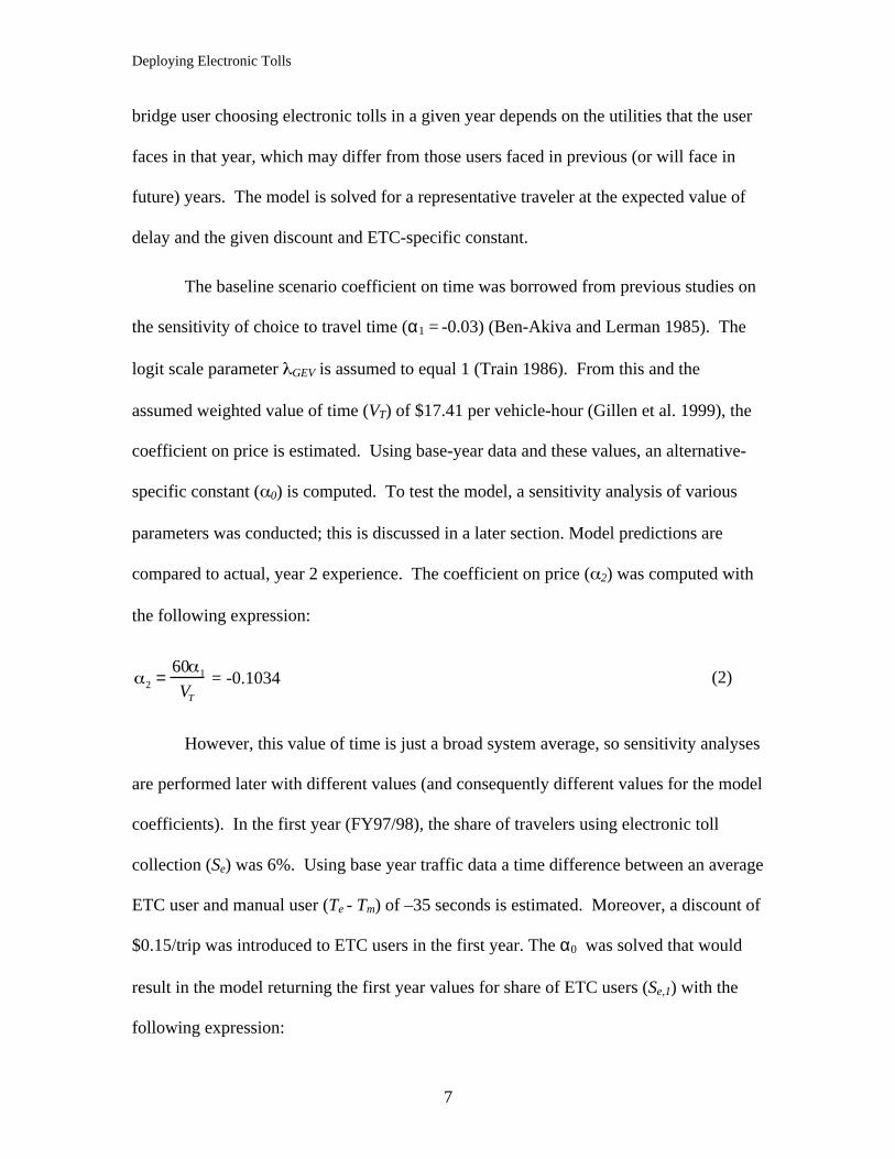
compared to actual, year 2 experience. The coefficient on price ( 2) was computed with

the following expression:

2 =

60 1

VT

= -0.1034 (2)

However, this value of time is just a broad system average, so sensitivity analyses

are performed later with different values (and consequently different values for the model

coefficients). In the first year (FY97/98), the share of travelers using electronic toll

collection (Se) was 6%. Using base year traffic data a time difference between an average

ETC user and manual user (Te - Tm) of –35 seconds is estimated. Moreover, a discount of

$0.15/trip was introduced to ETC users in the first year. The α0 was solved that would

result in the model returning the first year values for share of ETC users (Se,1) with the

following expression:


8

0 = ln

Se,1

1 − Se,1

− 1 ⋅ Te − Tm( ) − 2 Pe − Pm( ) = −3.08 (3)

Notice that the magnitude of ETC specific coefficient is much greater than the

other parameters. It means that a significant amount of savings in time and money is

needed to overcome the hurdle to adopt ETC technology. When the savings are

moderate, travelers would rather endure a slightly longer travel time than go through the

process of obtaining a transponder. However, when the savings are significant, or ETC is

required to obtain travel time savings as on SR 91 in Orange County California, or the

benefits are spread over multiple facilities (many toll facilities use the technology),

experience has shown that commuters will be more likely to use the new technology. To

illustrate, the Fastrak compatible Orange County's Transportation Corridor Agencies

routes have daily ETC use in excess of 50% and peak use in excess of 80% (ETTM

2001), while the compatible ETC system on the Golden Gate Bridge has over 40%

market share (Fimrite 2001).

Changing Dispositions toward ETC and Network Externalities

The constant ( 0) can be interpreted as a fixed cost associated with acquiring

transponders, implicitly a predisposition against switching from manual to ETC.

However, this disposition may not remain constant over time. There are several parallel

but offsetting processes going on.

In year 1, some fraction of the population chooses to adopt ETC. These early

adopters must have a smaller than average predisposition against the technology; that is

their constant ( 0adopt) is smaller in absolute terms. Thus those who don’t adopt in the


9

first year must have a greater than average value of the constant ( 0notadopt). In year 2, the

average predisposition against adoption rises even more among those who haven’t

adopted (all other things equal). However, it is impossible to know from the available

data how much higher the predisposition is, because there are many unknown factors

affecting payment choice in addition to variations in to the constant ( 0).

However, the willingness to try ETC may increase with the rate of adoption if

there exist any network externalities. These include multiple uses of transponders,

including toll plazas, parking garages, drive-through windows for fast food and gas at

service stations. Additional uses become increasingly viable the more existing uses and

users, and make acquiring a transponder that much more valuable. In addition, the longer

a system has been deployed, the more confidence potential users have in the system. In

general, as knowledge of a technology and realization of its benefits spreads, the rate of

adoption increases because each project acts as a demonstration to potential new users.

The net effect of these offsetting factors is unclear, so sensitivity tests will be

performed. First, as a default (baseline) assumption, ( 0) will simply be reduced from its

base year value to 0 in year 20 linearly. Second, for sensitivity analyses, ( 0) will be

multiplied by the share of manual users (Sm)z (where the power term z is sensitivity

variable) to see what happens to willingness to adopt as the background share of manual

users decreases from 100% in the base. This models the combined effect of the network

externality and individual predisposition.


10

Policy Variables: Capacity and Discount

According to the choice model, the toll agency can affect the evolution of ETC

share in several ways: providing a discount exclusively for ETC users; imposing

congestion in the manual lanes by supplying more ETC capacity than needed (and

reducing the capacity of manual lanes); and reducing the buy-in hurdle, the fixed cost

associated with ETC. In the basic model, the toll agency decides the discount and the

number of ETC lanes every year corresponding to the forecast ETC share that maximizes

the overall social welfare (the sum of benefits to the agency, commuters, and the

community, minus their costs, defined more precisely in the Appendix), such that ETC

delay is less than manual delay. However, this is myopic. By adding more ETC lanes

and closing manual lanes, travelers will switch to ETC payment and ETC market share

will grow. This may result in greater benefits in the end, despite deviating from the

short- run optimal. This issue would be eliminated if the model could solve the

optimization problem simultaneously over 20 years rather than sequentially year by year.

Unfortunately, an exact, non-heuristic, solution for the multi-year optimization is not

possible at this time due to the size of the problem, though some less myopic strategies in

the sensitivity analysis are examined below. Lanes are modeled as discrete, and

belonging to either manual or ETC. To illustrate the size of the problem, for 1 year the

agency must choose between 1 and 11 lanes (along with discounts). To optimize for 2

years, one has to choose over 112 lanes (the number of lanes in each year), so for 20 years

in principle, there are 1120 possible choices to optimize simultaneously (rather than 11x20

in the myopic optimization). While some simplifying assumptions such as irreversibility

may be made; nevertheless, it is a much larger problem to solve. It should be noted that


11

the model is insensitive to the engineering question of lane-location of ETC vs. Manual

lanes (i.e. should the ETC lanes be leftmost, rightmost, or in the center, or should they be

together or separated), which is an important question that would affect weaving at toll

plazas. While safety might be enhanced by allowing ETC in all lanes, time savings are

improved only if there are exclusive, non-stop ETC lanes.

Given the number of ETC lanes, annual traffic volume, and the dynamic payment

model, there is an optimal discount that maximizes the overall social welfare in any given

year. For each year 2 through 20, an optimal combination of ETC lanes and discount is

chosen to maximize the overall social welfare so long as the net benefit of the toll agency

is non-negative. This constraint is set to encourage the toll agency to implement the ETC

system, and may result in discontinuities in the optimization. Different buy-in hurdles

are tested in the sensitivity analysis.

Model System

Given the number of ETC lanes, discount policy and annual traffic volume, the

ETC market share is estimated from the payment choice model. Then, the costs incurred

and benefits gained for each class are calculated. An iterative procedure searches for the

optimal combination of ETC lane configuration (and thus delay) and discount policy to

maximize total social welfare given the market demand function.

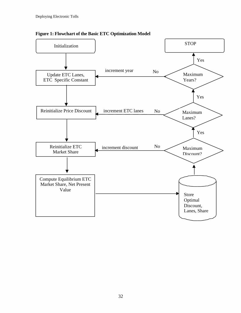
Figure 1 shows a flowchart that illustrates the model system. In the initialization

stage, the base year configuration of the toll plaza, survival rate, payment choice

parameters, and optimal discount are all established using the initial assumptions. The

equilibrium market share is computed using a grid search, establishing a market share

that would return traffic delays that result in the same market share, given a discount and


12

lane configuration. If the net present value from that configuration is better than all

previous NPVs for that year, the lane configuration and discount are stored as optimal;

otherwise, the previous optimal combination is retained. If the discount is not at a

maximum, it is incremented, and the process is repeated. If the number of lanes for ETC

is not at a maximum, the ETC lanes are incremented, and the process is repeated. At the

end of a year's trials, the information for that year is recorded, the optimal configuration

selected, and the model is run for the next year, through year 20.

Results

This section discusses the results. However, because each assumption is critical

to the results, sensitivity analyses are conducted in the next section to investigate how the

results depend on the initial assumptions.

Historical traffic and financial data at the Carquinez Bridge in northern California

are used to illustrate the procedure to determine an appropriate pace of ETC deployment

and discount policy. The Carquinez Bridge was selected as the ETC pilot

implementation in the San Francisco Bay Area because it has sufficient capacity to

accommodate current traffic (Gillen et al 1999). There are 12 lanes going through the toll

plaza. A dedicated ETC lane has been opened to travelers with transponders since

August 21, 1997. In addition, two lanes were opened for mixed ETC/Manual toll

collection. Since vehicles equipped with ETC suffer delay when the driver of the leading

vehicle pays the toll manually in mixed use lanes, the gains from mixed payment lanes

are expected to be marginal and are thus neglected in the model. Mixed lanes are treated

as manual lanes in this exercise and it is assumed that all vehicles equipped with

transponders only use the ETC-dedicated lane.


13

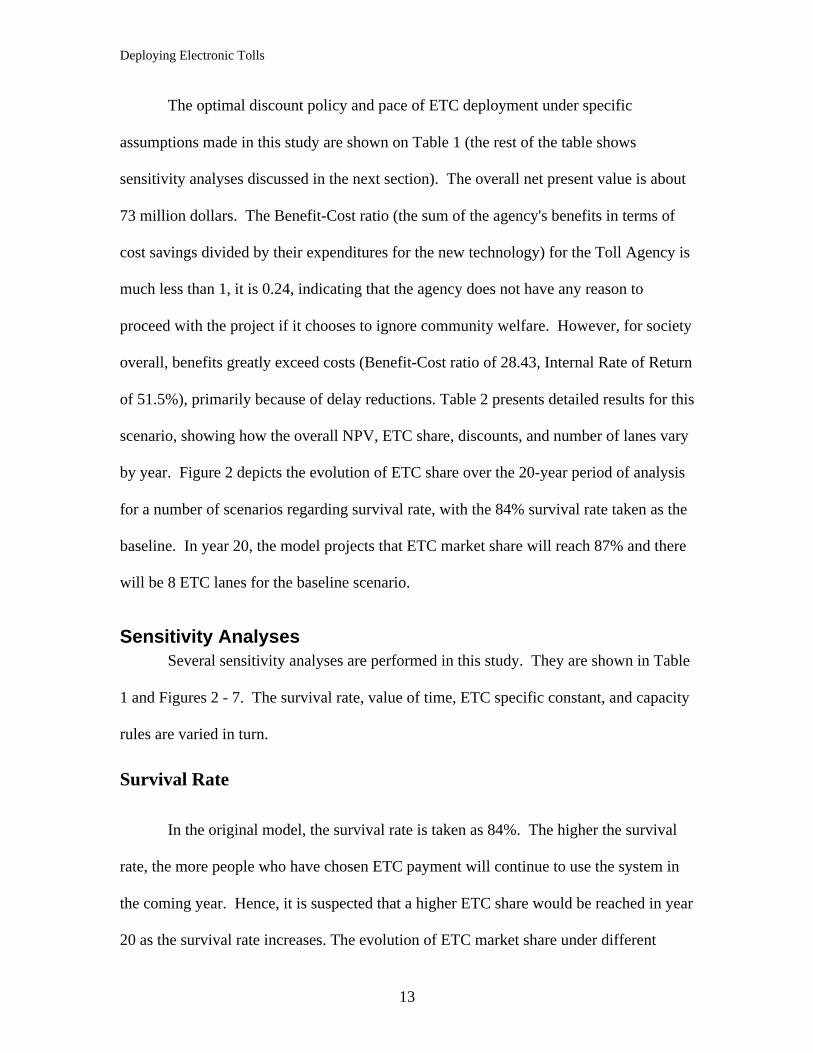
The optimal discount policy and pace of ETC deployment under specific

assumptions made in this study are shown on Table 1 (the rest of the table shows

sensitivity analyses discussed in the next section). The overall net present value is about

73 million dollars. The Benefit-Cost ratio (the sum of the agency's benefits in terms of

cost savings divided by their expenditures for the new technology) for the Toll Agency is

much less than 1, it is 0.24, indicating that the agency does not have any reason to

proceed with the project if it chooses to ignore community welfare. However, for society

overall, benefits greatly exceed costs (Benefit-Cost ratio of 28.43, Internal Rate of Return

of 51.5%), primarily because of delay reductions. Table 2 presents detailed results for this

scenario, showing how the overall NPV, ETC share, discounts, and number of lanes vary

by year. Figure 2 depicts the evolution of ETC share over the 20-year period of analysis

for a number of scenarios regarding survival rate, with the 84% survival rate taken as the

baseline. In year 20, the model projects that ETC market share will reach 87% and there

will be 8 ETC lanes for the baseline scenario.

Sensitivity AnalysesSeveral sensitivity analyses are performed in this study. They are shown in Table

1 and Figures 2 - 7. The survival rate, value of time, ETC specific constant, and capacity

rules are varied in turn.

Survival Rate

In the original model, the survival rate is taken as 84%. The higher the survival

rate, the more people who have chosen ETC payment will continue to use the system in

the coming year. Hence, it is suspected that a higher ETC share would be reached in year

20 as the survival rate increases. The evolution of ETC market share under different


14

survival rates is shown on Figure 2 (constrained so the annual NPV of the toll agency is

greater than zero).

As the survival rate falls, the operator has to provide greater incentives (via time

and money differentials) to achieve the same level of market share. An interesting (and

unexpected) behavior emerges for survival rates below 40%. The interplay of the overall

welfare optimization and two constraints (the operator has non-negative revenue and the

ETC lanes are always faster than the manual lanes) leads to what one might consider a

complex phase change. It seems that the toll agency chooses to allocate more ETC lanes

(11 in total) to enlarge the travel time difference between the two payment choices, and

this strategy brings about a higher market share in year 20 and a somewhat higher overall

NPV. This strategy of using the maximum number of ETC lanes does not maximize

welfare for higher survival rate cases. The comparison of NPV across different survival

rates is shown on Table 1, clearly the higher the survival rate, the higher the overall

market share and thus NPV.

Value of Time

In the original model, the value of time is taken as $17.41 per hr per vehicle. Two

alternative values of time also are tested, these are 10 times greater than and 10 times less

than the original value. While these may seem extreme, these numbers bound all

reasonable values of time. Furthermore, two other points are worth noting. First in the

absence of real time savings (i.e. in the absence of congestion), travel time hardly affects

the choice. Second, value of time affects the utility of both manual and electronic

payment. When travelers have a higher value of time, they are more sensitive to the

potential time saved by switching to ETC payment. It is expected that travelers would


15

adopt the ETC system earlier, and the final ETC market share is going to be higher, the

greater the value of time. The results shown on Figure 3 confirm the reasoning.

The market share under a high value of time exceeds that with lower values as

shown on Table 1. Although a radically lower value of time does not harm greatly the

pace of ETC adoption, the overall social welfare increases dramatically with the higher

value of time. As in the original model, travelers accrue the majority of benefits (original

model 102%, low value of time 103 %, high value of time 99%). Notice that the toll

agency also recovers its initial capital investment with a higher value of time. The early

realization of high ETC market share entitles the toll agency to enjoy significant cost

reductions, primarily toll collection staff, for a longer period.

Highly non-linear models of the logit form can yield biased results when applied

to average input values of independent variables. Sample enumeration can deal with the

actual distribution of commuters' values of time (Miller 1996, Ortuzar and Willumsen

1996, Purvis 1996). In principle, sample enumeration is preferred, however there are

several practical issues. The first is knowing the distribution of a representative sample.

In this case, the underlying distribution is unknown, all that is available is an estimate of

the average value of time for the population. While one could assume a distribution, that

would introduce a different set of errors. Second, this is a long-run analysis, so even if

the distribution were known, there is no assurance it would remain constant over time.

Third is the practical effect that such a change would produce. Experiments of doing a

sample enumeration approach on value of time show very little change. To test sample

enumeration, the value of time is varied between $1/hour and $34/hour (straddling the

assumed average ($17.41/hour), shown in Figure 4 (assuming base year, relatively


16

uncongested conditions). A uniform distribution of values of time between these two

values (an extreme case, as a real sample is likely to cluster about the mean) results in a

mean share of electronic tolls of 0.0502, rather than 0.0493 which obtained from simply

using the average value of time in the first place. A normal distribution would be even

closer to the original mean. As a result, it is concluded that over the range of values of

the variables in this paper, this simplification is unlikely to significantly bias the final

results.

ETC Specific Constant and Network Externalities

The reluctance to switch to ETC may decrease over time, but it is unclear how

quickly. In the original model it is posited that the ETC-specific constant ( 0) in the logit

choice model hits zero in year 20 by decreasing at a uniform rate. In this section,

different rates are investigated. Following the argument about network externalities, the

magnitude of this constant is associated with the share of ETC users (or nonusers). Here

α0=α0Smz , using the share of manual users (Sm) as a surrogate. The results of using

different power terms (z) are displayed in Figure 5.

For a number of years the power term results behave in an orderly way. Up to

year 12, the rankings in terms of market share are clearly proportional to the power term,

with higher positive power terms resulting in the highest share and lower negative power

terms resulting in the lowest share. A high power term means that positive feedback for

ETC is strong (a virtuous circle), users beget more users, and the magnitude of ETC-

specific constant (which is negative) falls quickly. A power term of 0 implies that there

are no feedback effects. A negative power term implies that the more existing ETC users

there are, the less likely new users will choose ETC.


17

However, the lower the power term (below 1), the sooner the agency will deploy

all 11 lanes. That is, when it must fight against a vicious circle to maximize welfare it

must make the choice of manual lanes less desirable due to high travel times. Also, the

lower the power term, the lower the final ETC market share.

The best available data for the Carquinez Bridge were used to estimate the real

value of the power term. The number of transponders at the Carquinez Bridge in year 2

is converted to get the approximate all-day market share, 9.2% for the second year. (The

baseline model had predicted a peak-period share of 11.54%, as shown in Table 2).

Assuming 6% market share for the first year, 84% survival rate, a 34.6-second difference

in travel time, and $0.15 discount for ETC users, the power term equals –1.636, and the

overall NPV for this scenario (as for any scenario with a negative power term) is

negative.

Two points should be noted about this unpleasant result. First, this paper models

the peak period, when more ETC travelers use the system, and then extrapolates that ETC

value to the non-peak to determine net benefit. The data are not broken down by

peak/non-peak. The market share should be higher during the peak period and the ETC-

specific constant should be lower than estimated. Secondly, maybe the reluctance is

really that strong. That means, the toll agency has to do something to affect people’s

preferences if it wants to proceed with ETC. Because the Carquinez ETC system was

initially considered a technology test rather than a market demonstration, very little effort

had been made to sell ETC to potential customers. The initial technological difficulties

and bad press associated with this particular experiment may contribute to the low ETC


18

share at the Carquinez Bridge (Nolte 1996). This may change significantly as ETC is

deployed at other San Francisco area toll bridges.

Alternative Capacity Rules

In the original model, the number of ETC (and non-ETC) lanes is decided by

optimizing overall NPV in a given year, independent of its consequences for future years.

As discussed in the last two sections, a greater number of ETC lanes is estimated to result

in higher overall NPV over the entire period. Is it possible to trade a suboptimal NPV in

the present year for a higher long-term NPV? The original capacity rule may be dubbed

“myopic optimization." Clearly, the best solution to this problem would be to optimize

the ETC allocation and price discount for all 20 years simultaneously. Due to constraints

on computation time, several heuristic alternatives were examined. The first heuristic,

specifies higher numbers of ETC lanes in the first year, and then estimates the number of

ETC lanes myopically. The second adapts the original capacity rule by adding one and

two more lanes to the myopic optimization results. In the third heuristic, referred to as

“bundling”, instead of the idealized 20 years, the number of ETC lanes and price discount

for two-year, three-year, and four-years are optimized simultaneously.

If travelers are forced to switch to ETC payment as early as possible, overall

social welfare over the 20 years may be greater. By forcing travelers to switch earlier,

future benefits may be realized earlier, at the expense of lower welfare in the first years.

In this simulation, the number of ETC lanes in the first year is fixed, and the same

myopic rule is applied afterwards. The evolution of ETC share with alternative capacity

rules is shown in Figure 6. Restricted by the condition that the NPV of the toll agency

must exceed zero, the maximum number of ETC lanes that can be deployed in the year


19

one is three. Interestingly, the saturated ETC market share converges to a certain range

in year 20 no matter the initial seed number of lanes. The maximum overall is attained

when two ETC lanes are installed in the first year.

The second rule adds one and two lanes to the number of ETC lanes computed

from the myopic optimization rules. The results for evolution of ETC share with

different capacity rules are shown on Figure 7. Again, the results confirm the early

observation that the earlier additional ETC lanes are deployed, the greater the overall

NPV is gained over the 20-year period.

Finally, the number of ETC lanes was optimized in two-, three-, and four-year

bundles, where all other assumptions are the same as in the original model. Figure 8

depicts the results. The longer time span taken into account, the higher overall welfare

attained compared to the myopic optimization rules. The welfare from a four-year

optimization is superior to the two-year optimization. The three-year bundle model

seems almost identical to the two-year bundle model. The gaps between two-, three-, and

four-year model are not as much as between the myopic and two-year model. It is likely

that the improvements one can obtain by optimization over longer time spans is limited,

and faces diminishing marginal returns.

Conclusions

The conversion of conventional toll plazas to electronic toll collection is

seemingly inevitable. How quickly it occurs remains to be seen. This paper examined a

process that may explain the speed of this conversion if public toll agencies strive to

improve the welfare for all year by year. It is clear that toll agency policy – by opening


20

ETC lanes sooner or later - can drive user adoption of ETC. Overall welfare is expected

to improve the greater the ETC market share, and the sooner that share is achieved.

Longer-term decision-making, as expected, will result in higher overall welfare than

myopic decisions, though the penalty for myopia (as high as 50%) depends on other

assumptions. Many of the gains can be achieved by simply looking two years ahead;

there appear to be diminishing returns to optimizing with an increasing number of years,

while modeling costs rise.

This paper modeled a particular case. As a matter of course, it has raised some

questions that are unable to be answered, but which are critical for strategic deployment

of network technologies such as ETC. In particular, there is the question of whether

individuals face positive network externalities associated with a technology or whether

their reluctance to make the leap is wider. While the second year of data for the

Carquinez Bridge suggest the latter, that data is associated with little marketing as the

agency attempts to ensure the technology is working smoothly. A more concerted

marketing strategy to reduce the barriers to entry could easily shift preferences.

Furthermore, deployment of ETC on other Bay Area bridges should also create a positive

externality. Alternatively, use of Automatic Vehicle Identification, such as used on

Highway 407 in Toronto, which eliminates the transponder buy-in, may be an alternative.

Clearly, more empirical research is needed on user preferences for this and other new

technologies, to ascertain which deployment scenario is most reasonable.

The single most important factor in the model that dictates if ETC fails or

flourishes is whether the barrier to entry rises or falls over time. If additional users, or


21

other factors, diminish the barrier, the system will take off. If they do not, those

predisposed against ETC will adopt it at a smaller and smaller rate each successive year.


22

Appendix: Benefits and Costs of ETCTo estimate the costs and benefits, a number of basic assumptions are made.

These include overall traffic growth, toll transaction time by type of payment, travel

speed, design configuration of Carquinez Bridge, annual inflation rate and interest rate.

The main assumptions are listed in Table A1 and explained below.

This framework identifies benefit and cost categories for Travelers (Time,

Vehicle Operating Costs), Agencies (Fixed & Operating Costs of Toll Collection,

Revenue), and the Community (Pollution). While the measure of overall net present

value (NPV) ignores transfers, they are considered for the NPV of each user class.

Transfers include tolls paid (a transfer from the user to the toll agency), or interest on

prepaid ETC credit accounts (lost to travelers but accrued to the agency). Inflation of 3%

per year is assumed for all costs and money values, before discounting back to the present

with an interest rate of 6% and discount rate of 3%.

Costs and benefits for each class (travelers, the toll agency, and the community)

can be estimated separately. The overall social welfare (W) is defined as:

W = BT − CT + BA − CA + BC − CC (A1)

Where:

BA, BC, BT benefits for the toll agency, the community, and travelers

CA, CC, CT costs for the toll agency, the community, and travelers

Travelers

Travelers are divided into two classes, referred to as manual and electronic. Cost

savings for electronic travelers come from reduced delay because of higher throughputs


23

on ETC lanes, and elimination of acceleration and deceleration processes associated with

manual toll collections. For the convenience of analysis, it is assumed that the value of

time, the mode split (car, truck, bus), and the average vehicle occupancy do not vary over

the analysis period.

Delay

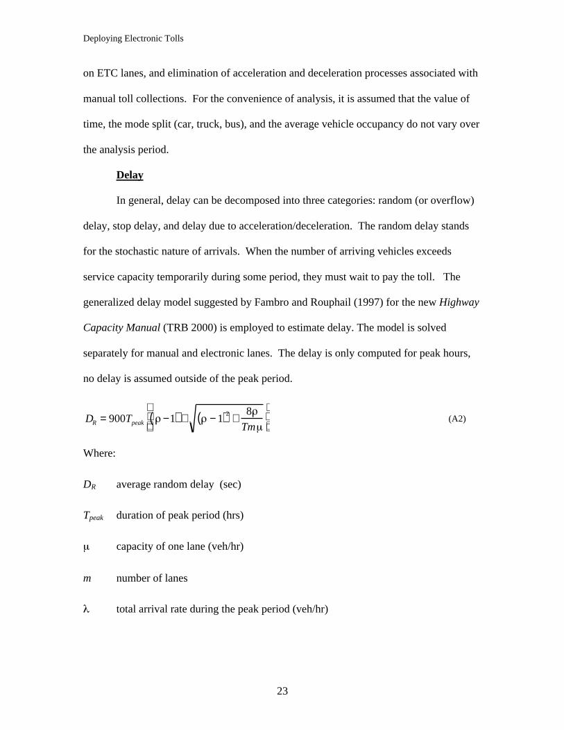
In general, delay can be decomposed into three categories: random (or overflow)

delay, stop delay, and delay due to acceleration/deceleration. The random delay stands

for the stochastic nature of arrivals. When the number of arriving vehicles exceeds

service capacity temporarily during some period, they must wait to pay the toll. The

generalized delay model suggested by Fambro and Rouphail (1997) for the new Highway

Capacity Manual (TRB 2000) is employed to estimate delay. The model is solved

separately for manual and electronic lanes. The delay is only computed for peak hours,

no delay is assumed outside of the peak period.

DR = 900Tpeak −1( ) + − 1( )2 +8

Tm

(A2)

Where:

DR average random delay (sec)

Tpeak duration of peak period (hrs)

capacity of one lane (veh/hr)

m number of lanes

total arrival rate during the peak period (veh/hr)


24

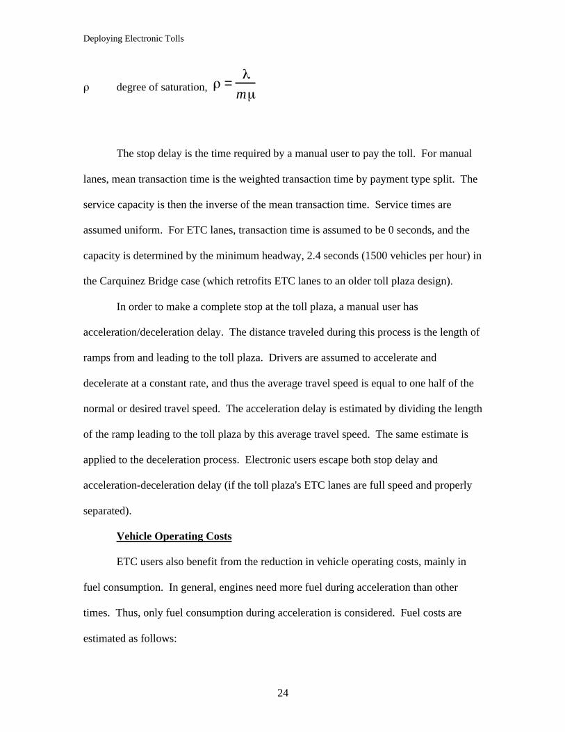
degree of saturation, =m

The stop delay is the time required by a manual user to pay the toll. For manual

lanes, mean transaction time is the weighted transaction time by payment type split. The

service capacity is then the inverse of the mean transaction time. Service times are

assumed uniform. For ETC lanes, transaction time is assumed to be 0 seconds, and the

capacity is determined by the minimum headway, 2.4 seconds (1500 vehicles per hour) in

the Carquinez Bridge case (which retrofits ETC lanes to an older toll plaza design).

In order to make a complete stop at the toll plaza, a manual user has

acceleration/deceleration delay. The distance traveled during this process is the length of

ramps from and leading to the toll plaza. Drivers are assumed to accelerate and

decelerate at a constant rate, and thus the average travel speed is equal to one half of the

normal or desired travel speed. The acceleration delay is estimated by dividing the length

of the ramp leading to the toll plaza by this average travel speed. The same estimate is

applied to the deceleration process. Electronic users escape both stop delay and

acceleration-deceleration delay (if the toll plaza's ETC lanes are full speed and properly

separated).

Vehicle Operating Costs

ETC users also benefit from the reduction in vehicle operating costs, mainly in

fuel consumption. In general, engines need more fuel during acceleration than other

times. Thus, only fuel consumption during acceleration is considered. Fuel costs are

estimated as follows:


25

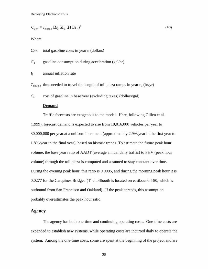
CGTn = Tplaza, n ⋅ Ga ⋅CG ⋅(1+ I f )n (A3)

Where

CGTn total gasoline costs in year n (dollars)

Ga gasoline consumption during acceleration (gal/hr)

If annual inflation rate

Tplaza,n time needed to travel the length of toll plaza ramps in year n, (hr/yr)

CG cost of gasoline in base year (excluding taxes) (dollars/gal)

Demand

Traffic forecasts are exogenous to the model. Here, following Gillen et al.

(1999), forecast demand is expected to rise from 19,016,000 vehicles per year to

30,000,000 per year at a uniform increment (approximately 2.9%/year in the first year to

1.8%/year in the final year), based on historic trends. To estimate the future peak hour

volume, the base year ratio of AADT (average annual daily traffic) to PHV (peak hour

volume) through the toll plaza is computed and assumed to stay constant over time.

During the evening peak hour, this ratio is 0.0995, and during the morning peak hour it is

0.0277 for the Carquinez Bridge. (The tollbooth is located on eastbound I-80, which is

outbound from San Francisco and Oakland). If the peak spreads, this assumption

probably overestimates the peak hour ratio.

Agency

The agency has both one-time and continuing operating costs. One-time costs are

expended to establish new systems, while operating costs are incurred daily to operate the

system. Among the one-time costs, some are spent at the beginning of the project and are


26

independent of the number of open lanes and traffic level. The costs of installing

additional ETC lanes and purchasing transponders are allocated to the year associated

with the incremental increase in ETC users.

The operating costs can be divided into three categories: staffing,

hardware/software, and other. Staffing is comprised of employees in information

technology, accounting, and toll collection. Personnel costs for information technology

(YI) and accounting (YA) are assumed constant over time (Caltrans 1995). Only toll

collection personnel (YTn) vary with manual traffic volume, so those are estimated by the

model. A promising cost savings for the toll agency from adopting the ETC alternative is

the reduction in toll collection staff, proportionate to the number of manual lanes. Staff

costs are estimated by multiplying the personnel needed for each alternative and the cost

per person. The number of persons needed for toll collection can be estimated given

forecast annual traffic volume and ETC market share. The costs of staffing can be

obtained as follows.

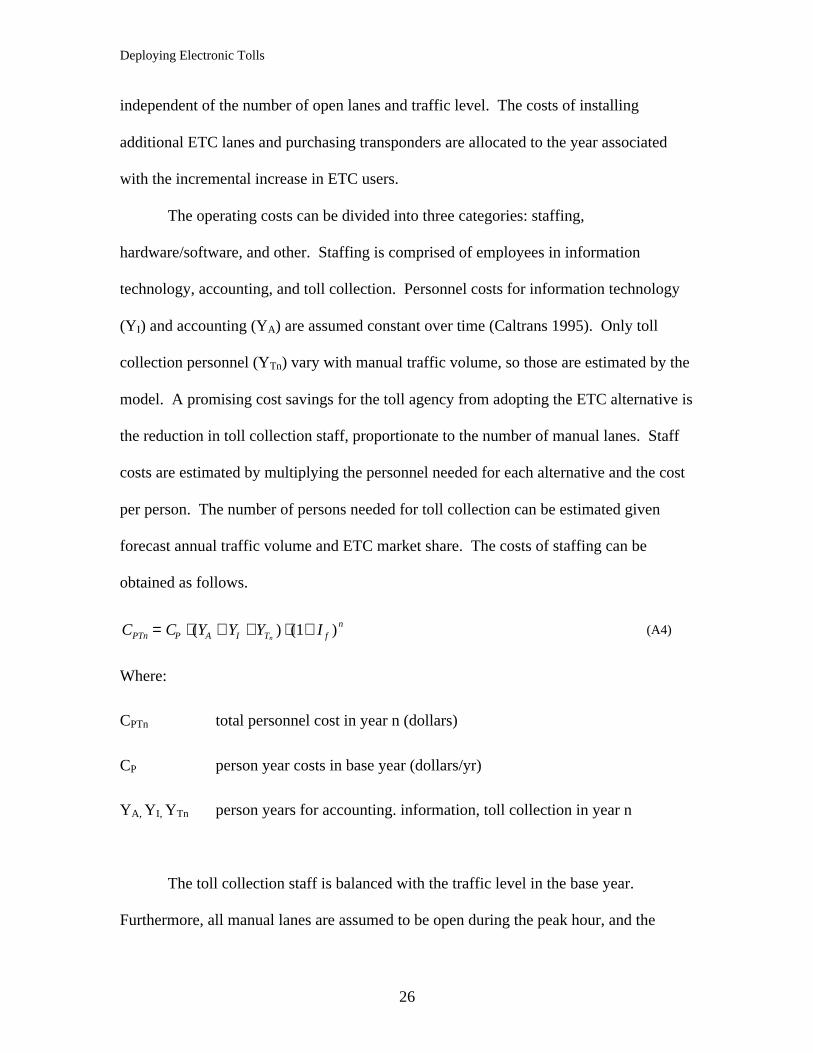
CPTn = CP ⋅ (YA + YI +YTn) ⋅ (1+ I f )n (A4)

Where:

CPTn total personnel cost in year n (dollars)

CP person year costs in base year (dollars/yr)

YA, YI, YTn person years for accounting. information, toll collection in year n

The toll collection staff is balanced with the traffic level in the base year.

Furthermore, all manual lanes are assumed to be open during the peak hour, and the


27

personnel needed during the off-peak period is proportional to the number of manual

transactions during the off-peak. Off-peak traffic is estimated by subtracting projected

annual peak traffic from the projected annual traffic volume. In this model the ETC share

is the same during the peak and off-peak period. However, it might be more realistic to

expect that the ETC share will be higher during the peak hours when significant time may

be saved, and because peak travelers are more regular users of the system.

Hardware/software costs for information technology and other program costs are

estimated from the ATCAS Report (Caltrans 1995).

Community

The primary benefit of ETC systems to communities at large is the reduction of

NOx, HC, and CO emission during idling and acceleration. The magnitude of the

emissions impacts are small however, compared with the other impact dimensions.

Emission rates are given in Table A1. Total emissions of pollutant p from idling in year

n (EidleT,p,n), (in gm) are estimated as follows.

EidleT , p,n = Tidle, n ⋅ Eidle, p ⋅ 60 (A5)

Wher e:

Tidle,n time idling in year n (hr)

Eidle, p emission rate for pollutant type p during idling (gm/min)

Total emissions of pollutant p from acceleration in year n (EaccT,p,n) (in gm) are:

EaccT, p,n = (Tplaza,n) ⋅ Ga ⋅ Eacc, p (A6)

Wher e:


28

Eacc,p emission rate of pollutant type p during acceleration (gm/gal)

Ga fuel consumption rate during acceleration (gal/hr)


29

References

Al-Deek, H. M. A.E. Radwan, A.A. Mohammed And J.G. Klodzinski. 1996. “EvaluatingThe Improvements In Traffic Operations At A Real-Life Toll Plaza WithElectronic Toll Collection.” ITS Journal, Vol. 3(3), , Pp. 205-223.

Al-Deek, H.M.; A.A. Mohamed,; A.E. Radwan. 1997. Operational Benefits Of ElectronicToll Collection: Case Study. Journal Of Transportation Engineering, V123, N6Nov-Dec,

Asahi Shimbun. 2001. "Ministry to slash electronic toll fees" August 1, 2001, appearingin English Language supplement of Asahi Shimbun to International HeraldTribune

Ben-Akiva M. and S. Lerman 1985 Discrete Choice Analysis, MIT Press, CambridgeMA

Burris M; E. Hildebrand 1996. Using Microsimulation To Quantify The Impact OfElectronic Toll Collection ITE Journal V66 N7 :21-24.

California Department Of Transportation (Caltrans). 1995. Advanced Toll CollectionAnd Accounting System (ATCAS) Feasibility Study Report. TIRU Project #2400-146.

California Department Of Transportation (Caltrans). 1995. Annual Financial Report:State Owned Toll Bridges

Chang, Elva Chia-Huei, David Levinson, And David Gillen 1998. User’s Manual ForComputerized Benefit-Cost Analysis Of Electronic Toll Collection System(October 28 1998) Filed As Part Of MOU-357

Cicero-Fernandez, P., and J. Long. "Modal Acceleration Testing on CurrentTechnology Vehicles." California Air Research Board, El Monte California,1993.

ETTM. 2001 Table: United States ETC Systems In Production / Developmenthttp://www.ettm.com/

Fambro, D. B.; N. M. Rouphail 1997. Generalized Delay Model For SignalizedIntersections And Arterial Streets. Transportation Research Record 1572.

Federal Highway Administration, U.S. DOT. 1996. "Highway EconomicRequirements System, Volume IV: Technical Report." DOT-VNTSC-FHWA-96-6, p. 8-28.

Fimrite Peter. 2001. "FasTrak Putting The Brakes On Golden Gate Bridge Discounts"Originally posted in: The San Francisco Chronicle June 29, 2001

Friedman, David A.; Waldfogel, Joel 1995. The Administrative And Compliance Cost OfManual Highway Toll Collection: Evidence From Massachusetts And NewJersey. National Tax Journal, V48, N2 :217-228.


30

Gillen, David Jianling Li, Joy Dahlgren, Elva Chang. 1999. Assessing the Benefits andCosts of ITS Projects: Volume 2 An Application to Electronic Toll Collection.California PATH Research Report UCB-ITS-PRR-99-10

Hensher David. 1991. Electronic Toll Collection Transportation Research Part A-General, Jan, , 25:1 9-16.

Levinson, David M. 1997. Job And Housing Tenure And The Journey To Work. AnnalsOf Regional Science 31:4 451-471.

Lin, Feng-Bor And Cheng-Wei Su. 1994. “Level-Of-Service Analysis Of Toll Plazas OnFreeway Main Lines.” Journal Of Transportation Engineering, 120:2 246-263.

Miller Eric J., 1996. "Microsimulation and Activity-Based Forecasting." Activity-BasedTravel Forecasting Conference Proceedings June 2-5, 1996 Summary,Recommendations and Compendium of Papers February 1997http://www.bts.gov/tmip/papers/tmip/abtf/miller.htm

Nolte, Carl. 1996. "Automatic Tollbooth Technology Not Yet Ready for Prime Time"San Francisco Chronicle September 23, 1996

Ortuzar, Juan de Dios and Luis Willumsen. 1996. Modelling Transport. John Wiley andSon, Ltd

Purvis, Charles L. 1996. "Use of Census Data in Transportation Planning: San FranciscoBay Area Case Study" Decennial Census Data for Transportation Planning: CaseStudies and Strategies for 2000: Conference Proceedings 13, Volume 2, NationalAcademy Press, Washington, D.C., 1997, pp. 58-67http://www.mtc.ca.gov/datamart/census/irvine96.htm

Robinson, Mark And Michel Van Aerde. 1995. “Examining The Delay AndEnvironmental Impacts Of Toll Plaza.” In 1995 Vehicle Navigation &Information Systems Conference Proceedings - 6th International VNIS, July 30 -August 2, 1995, Washington State Convention And Trade Center, Seattle ,Washington, USA.

Sisson, Mark. 1995. Air Quality Benefits Of Electronic Toll Collection. TransportationQuarterly, V49, N4 93

Small, Kenneth A, and Camilla Kazimi. 1995. "On the Costs of Air Pollution fromMotor Vehicles," Journal of Transport Economics and Policy, Jan. 1995, pp.7-32.

Train, Kenneth. 1986. Qualitative Choice Analysis. MIT Press. Cambridge MA

Transportation Research Board. 2000. Highway Capacity Manual, Special Report 209.Transportation Research Board Washington DC

Woo, T. Hugh And Lester A. Hoel. 1991. “An Investigation Of Toll Plaza Capacity AndLevel Of Service.” Virginia Transportation Research Council.

Zarrillo, M; Radwan, A; Al-Deek, H. 1997. Modeling Traffic Operations At ElectronicToll Collection And Traffic Management Systems Computers & IndustrialEngineering, V33 N3-4 :857-860.


31


32

Figu re 1: Flow chart of t he Basic ETC Op tim ization Model

No

Yes

Yes

Compute Equilibrium ETCMarket Share, Net Present

Value

Reinitialize ETCMarket Share

increment discount

Update ETC Lanes,ETC Specific Constant

Reinitialize Price Discount increment ETC lanes

increment year No

No

Yes

StoreOptimalDiscount,Lanes, Share

MaximumDiscount?

MaximumLanes?

MaximumYears?

Yes

STOPInitialization

Documents

A Model for Optimizing Electronic Toll Collection Systems · PDF fileDeploying Electronic Tolls 2 Introduction Newly deployed electronic toll collection (ETC) systems enable bridge,