Under review as a conference paper at ICLR 2017

A NEURAL STOCHASTIC VOLATILITY MODEL

Rui Luo†, Xiaojun Xu‡, Weinan Zhang‡, Jun Wang††University College London, ‡Shanghai Jiao Tong University{r.luo,j.wang}@cs.ucl.ac.uk, {xuxj,wnzhang}@apex.sjtu.edu.cn

ABSTRACT

In this paper, we show that the recent integration of statistical models with re-current neural networks provides a new way of formulating volatility models thathave been popular in time series analysis and prediction. The model comprises apair of complementary stochastic recurrent neural networks: the generative net-work models the joint distribution of the stochastic volatility process; the inferencenetwork approximates the conditional distribution of the latent variables given theobservable ones. Our focus in this paper is on the formulation of temporal dynam-ics of volatility over time under a stochastic recurrent neural network framework.Our derivations show that some popular volatility models are a special case ofour proposed neural stochastic volatility model. Experiments demonstrate thatthe proposed model generates a smoother volatility estimation, and outperformsstandard econometric models GARCH, EGARCH, GJR-GARCH and some otherGARCH variants as well as MCMC-based model stochvol and a recent Gaussianprocesses based volatility model GPVOL on several metrics about the fitness ofthe volatility modelling and the accuracy of the prediction.

1 INTRODUCTION

The volatility of the price movements reflects the ubiquitous uncertainty within financial markets. Itis critical that the level of risk, indicated by volatility, is taken into consideration before investmentdecisions are made and portfolio are optimised (Hull, 2006); volatility is substantially a key variablein the pricing of derivative securities. Hence, estimating and forecasting volatility is of great im-portance in branches of financial studies, including investment, risk management, security valuationand monetary policy making (Poon & Granger, 2003).

Volatility is measured typically by using the standard deviation of price change in a fixed time in-terval, such as a day, a month or a year. The higher the volatility, the riskier the asset. One ofthe primary challenges in designing volatility models is to identify the existence of latent (stochas-tic) variables or processes and to characterise the underlying dependences or interactions betweenvariables within a certain time span. A classic approach has been to handcraft the characteris-tic features of volatility models by imposing assumptions and constraints, given prior knowledgeand observations. Notable examples include autoregressive conditional heteroskedasticity (ARCH)model (Engle, 1982) and its generalisation GARCH (Bollerslev, 1986), which makes use of autore-gression to capture the properties of time-variant volatility within many time series. Heston (1993)assumed that the volatility follows a Cox-Ingersoll-Ross (CIR) process (Cox et al., 1985) and de-rived a closed-form solution for options pricing. While theoretically sound, those approaches requirestrong assumptions which might involve complex probability distributions and non-linear dynamicsthat drive the process, and in practice, one may have to impose less prior knowledge and rectify asolution under the worst-case volatility case (Avellaneda & Paras, 1996).

In this paper, we take a fully data driven approach and determine the configurations with as fewexogenous input as possible, or even purely from the historical data. We propose a neural networkre-formulation of stochastic volatility by leveraging stochastic models and recurrent neural networks(RNNs). We are inspired by the recent development on variational approaches of stochastic (deep)neural networks (Kingma & Welling, 2013; Rezende et al., 2014) to a recurrent case (Chung et al.,2015; Fabius & van Amersfoort, 2014; Bayer & Osendorfer, 2014), and our formulation shows thatexisting volatility models such as the GARCH (Bollerslev, 1986) and the Heston model (Heston,1993) are the special cases of our neural stochastic volatility formulation. With the hidden latent

1

Under review as a conference paper at ICLR 2017

variables in the neural networks we naturally uncover the underlying stochastic process formulatedfrom the models.

Experiments with synthetic data and real-world financial data are performed, showing that the pro-posed model outperforms the widely-used GARCH model on several metrics of the fitness and theaccuracy of time series modelling and prediction: it verifies our model’s high flexibility and richexpressive power.

2 RELATED WORK

A notable volatility method is autoregressive conditional heteroskedasticity (ARCH) model (En-gle, 1982): it can accurately capture the properties of time-variant volatility within many types oftime series. Inspired by ARCH model, a large body of diverse work based on stochastic processfor volatility modelling has emerged. Bollerslev (1986) generalised ARCH model to the gener-alised autoregressive conditional heteroskedasticity (GARCH) model in a manner analogous to theextension from autoregressive (AR) model to autoregressive moving average (ARMA) model byintroducing the past conditional variances in the current conditional variance estimation. Engle& Kroner (1995) presented theoretical results on the formulation and estimation of multivariateGARCH model within simultaneous equations systems. The extension to multivariate model allowsthe covariances to present and depend on the historical information, which are particularly useful inmultivariate financial models. Heston (1993) derived a closed-form solution for option pricing withstochastic volatility where the volatility process is a CIR process driven by a latent Wiener processsuch that the current volatility is no longer a deterministic function even if the historical informationis provided. Notably, empirical evidences have confirmed that volatility models provide accurateforecasts (Andersen & Bollerslev, 1998) and models such as ARCH and its descendants/variantshave become indispensable tools in asset pricing and risk evaluation.

On the other hand, deep learning (LeCun et al., 2015; Schmidhuber, 2015) that utilises nonlinearstructures known as deep neural networks, powers various applications. It has triumph over patternrecognition challenges, such as image recognition (Krizhevsky et al., 2012; He et al., 2015; van denOord et al., 2016), speech recognition (Hinton et al., 2012; Graves et al., 2013; Chorowski et al.,2015), machine translation (Sutskever et al., 2014; Cho et al., 2014; Bahdanau et al., 2014; Luonget al., 2015) to name a few.

Time-dependent neural networks models include RNNs with advanced neuron structure such as longshort-term memory (LSTM) (Hochreiter & Schmidhuber, 1997), gated recurrent unit (GRU) (Choet al., 2014), and bidirectional RNN (BRNN) (Schuster & Paliwal, 1997). Recent results show thatRNNs excel for sequence modelling and generation in various applications (Graves, 2013; Gregoret al., 2015). However, despite its capability as non-linear universal approximator, one of the draw-backs of neural networks is its deterministic nature. Adding latent variables and their processes intoneural networks would easily make the posterori computationally intractable. Recent work showsthat efficient inference can be found by variational inference when hidden continuous variables areembedded into the neural networks structure (Kingma & Welling, 2013; Rezende et al., 2014). Someearly work has started to explore the use of variational inference to make RNNs stochastic (Chunget al., 2015; Bayer & Osendorfer, 2014; Fabius & van Amersfoort, 2014). Bayer & Osendorfer(2014) and Fabius & van Amersfoort (2014) considered the hidden variables are independent be-tween times, whereas (Fraccaro et al., 2016) utilised a backward propagating inference networkaccording to its Markovian properties. Our work in this paper extends the work (Chung et al., 2015)with a focus on volatility modelling for time series. We assume that the hidden stochastic variablesfollow a Gaussian autoregression process, which is then used to model both the variance and themean. We show that the neural network formulation is a general one, which covers two major fi-nancial stochastic volatility models as the special cases by defining the specific hidden variables andnon-linear transforms.

3 PRELIMINARY: VOLATILITY MODELS

Stochastic processes are often defined by stochastic differential equations (SDEs), e.g. a (univariate)generalised Wiener process is dxt = µd t + σ dwt, where µ and σ denote the time-invariant ratesof drift and standard deviation (square root of variance) while dwt ∼ N (0,d t) is the increment of

2

Under review as a conference paper at ICLR 2017

standard Wiener process at time t. In a small time interval between t and t+∆t, the change in thevariable is ∆xt = µ∆t+ σ∆wt. Let ∆t = 1, we obtain the discrete-time version of basic volatilitymodel:

xt = xt−1 + µ+ σεt, (1)

where εt ∼ N (0, 1) is a sample drawn from standard normal distribution. In the multivariate case,Σrepresents the covariance matrix in place of σ2. As presumed that the variables are multidimensional,we will useΣ to represent variance in general case except explicitly noted.

3.1 DETERMINISTIC VOLATILITY

The time-invariant variance Σ can be extended to be a function Σt = Σ(x<t) relying on historyof the (observable) underlying stochastic process {x<t}. The current variance Σt is therefore de-termined given the history {x<t} up to time t. An example of such extensions is the univariateGARCH(1,1) model (Bollerslev, 1986):

σ2t = α0 + α1(xt−1 − µt−1)

2 + β1σ2t−1, (2)

where xt−1 is the observation from N (µt−1, σ2t−1) at time t − 1. Note that the determinism is in

a conditional sense, which means that it only holds under the condition that the complete history{x<t} is presented, such as the case of 1-step-ahead forecast. otherwise the current volatility wouldstill be stochastic as it is built on stochastic process {xt}. However, for multi-step-ahead forecast, weusually exploit the relation Et−1[(xt−µt)

2] = σ2t to substitute the corresponding terms and calculate

the forecasts with longer horizon in a recursive fashion, for example, σ2t+1 = α0 + α1Et−1[(xt −

µt)2] + β1σ

2t = α0 + (α1 + β1)σ

2t . For n-step-ahead forecast, there will be n iterations and the

procedure is hence also deterministic.

3.2 STOCHASTIC VOLATILITY

Another extension is applicable for Σt from being conditionally deterministic (i.e. deterministicgiven the complete history {x<t}) to fully stochastic: Σt = Σ(z≤t) is driven by another latentstochastic process {zt} instead of the observable process {xt}. Heston (1993) model instantiates acontinuous-time stochastic volatility model for univariate processes:

dxt = (µ− 0.5σ2t ) d t+ σt dw

〈1〉t , (3)

dσt = aσt d t+ bdw〈2〉t , (4)

where the correlation between dw〈1〉t and dw

〈2〉t applies: E[dw〈1〉t ·dw

〈2〉t ] = ρd t. We apply Euler’s

scheme of quantisation (Stoer & Bulirsch, 2013) to obtain the discrete analogue to the continuous-time Heston model (Eqs. (3) and (4)):

xt = (xt−1 + µ− 0.5σ2t ) + σεt

σt = (1 + a)σt−1 + bztwhere

[εtzt

]= N (0,

[1 ρρ 1

]). (5)

3.3 VOLATILITY MODEL IN GENERAL

As discussed above, the observable variable xt follows Gaussian distribution of which the mean andvariance depend on the history of observable process {xt} and latent {zt}. We presume in additionthat the latent process {zt} is an autoregressive model such that zt is (conditionally) Gaussiandistributed. Therefore, we formulate the volatility model in general as:

zt ∼ N (µz(z<t),Σz(z<t)), (6)

xt ∼ N (µx(x<t, z≤t),Σx(x<t, z≤t)), (7)

where µz(x<t, z≤t) and Σz(x<t, z≤t) denote the autoregressive time-varying mean and varianceof the latent variable zt while µx(x<t, z≤t) and Σx(x<t, z≤t) represent the mean and variance ofobservable variable xt, which depend on not only history of the observable process {x<t} but thatof the latent process {z≤t}.These two formulas (Eqs. (6) and (7)) abstract the generalised formulation of volatility models.Together, they represents a broad family of volatility models with latent variables, where the Heston

3

Under review as a conference paper at ICLR 2017

model for stochastic volatility is merely a special case of the family. Furthermore, it will degenerateto deterministic volatility models such as the well-studied GARCH model if we disable the latentprocess.

4 NEURAL STOCHASTIC VOLATILITY MODELS

In this section, we establish the neural stochastic volatility model (NSVM) for stochastic volatilityestimation and forecast.

4.1 GENERATING OBSERVABLE SEQUENCE

Recall that the latent variable zt (Eq. (6)) and the observable xt (Eq. (7)) are described by autore-gressive models (xt has the exogenous input {z≤t}.) For the distributions of {zt} and {xt}, thefollowing factorisation applies:

pΦ(Z) =∏t

pΦ(zt|z<t) =∏t

N (zt;µzΦ(z<t),Σ

zΦ(z<t)), (8)

pΦ(X|Z) =∏t

pΦ(xt|x<t, z≤t) =∏t

N (xt;µxΦ(x<t, z≤t),Σ

xΦ(x<t, z≤t)), (9)

where X = {xt} and Z = {zt} are the sequences of observable and latent variables, respectively,while Φ represents the parameter set of the model. The full generative model is defined as the jointdistribution:

pΦ(X,Z) =∏t

pΦ(xt|x<t, z≤t)pΦ(zt|z<t)

=∏t

N (zt;µzΦ(z<t),Σ

zΦ(z<t))N (xt;µ

xΦ(x<t, z≤t),Σ

xΦ(x<t, z≤t)). (10)

It is observed that the means and variances are conditionally deterministic: given the historicalinformation {z<t}, the current mean µz

t = µzΦ(z<t) and varianceΣz

t = ΣzΦ(z<t) of zt is obtained

and hence the distribution N (zt;µzt ,Σ

zt ) of zt is specified; after sampling zt from the specified

distribution, we incorporate {x<t} and calculate the current meanµxt = µx

Φ(x<t, z≤t) and varianceΣx

t = ΣxΦ(x<t, z≤t) of xt and determine its distribution N (xt;µ

xt ,Σ

xt ) of xt. It is natural and

convenient to present such a procedure in a recurrent fashion because of its autoregressive nature.As is known that RNNs can essentially approximate arbitrary function of recurrent form (Hammer,2000), the means and variances, which may be driven by complex non-linear dynamics, can beefficiently computed using RNNs.

It is always a good practice to reparameterise the random variables before we go into RNN ar-chitecture. As the covariance matrix Σ is symmetric and positive definite, it can be factorisedas Σ = UΛU>, where Λ is a full-rank diagonal matrix with positive diagonal elements. LetA = UΛ

12 , we have Σ = AA>. Hence we can reparameterise the latent variable zt (Eq. (6)) and

observable xt (Eq. (7)):

zt = µzt +A

zt ε

zt , (11)

xt = µxt +Ax

t εxt , (12)

where Azt (A

zt )> = Σz

t ,Axt (A

xt )> = Σx

t and εxt ∼ N (0, Ix), εzt ∼ N (0, Iz) are auxiliary vari-

ables. Note that the randomness within the variables of interest (e.g. zt) is extracted by the auxiliaryvariables (e.g. εt) which follow the standard distributions. Hence, the reparameterisation guaranteesthat gradient-based methods can be applied in learning phase (Kingma & Welling, 2013).

In this paper, the joint generative model is comprised of two sets of RNN and multilayer perceptron(MLP): RNNz

g/MLPzg for the latent variable, while RNNx

g /MLPzg for the observables. We stack

these two RNN/MLP together according to the causal dependency between those variables. The

4

Under review as a conference paper at ICLR 2017

joint generative model is implemented as the generative network:

{µzt ,A

zt } = MLPz

g(hzt ;Φ), (13)

hzt = RNNz

g(hzt−1, zt−1;Φ), (14)

zt = µzt +A

zt ε

zt , (15)

{µxt ,A

xt } = MLPx

g(hxt ;Φ), (16)

hxt = RNNx

g(hxt−1,xt−1, zt;Φ), (17)

xt = µxt +Ax

t εxt , (18)

where hzt and hx

t denote the hidden states of the corresponding RNNs. The MLPs map the hiddenstates of RNNs into the means and deviations of variables of interest. The parameter set Φ iscomprised of the weights of RNNs and MLPs.

One should notice that when the latent variable z is obtained, e.g. by inference (details in the nextsubsection), the conditional distribution pΦ(X|Z) (Eq. (9)) will involve in generating the observablext instead of the joint distribution pΦ(X,Z) (Eq. (10)). This is essentially the scenario of predictingfuture values of the observable variable given its history. We will use the term “generative model”and will not discriminate the joint generative model or the conditional one as it can be inferred incontext.

4.2 INFERENCING THE LATENT PROCESS

As the generative model involves latent variable zt, of which the true valus are unaccessible even wehave observed xt. Hence, the marginal likelihood pΦ(X) becomes the key that bridges the modeland the data. The calculation of marginal likelihood involves the posterior distribution pΦ(Z|X),which is often intractable as complex integrals are involved. We are unable to learn the paramtersor to infer the latent variables. Therefore, we consider instead a restricted family of tractable dis-tributions qΨ(Z|X), referred to as the approximate posterior family, as approximations to the trueposterior pΦ(Z|X) such that the family is sufficiently rich and flexible to provide good approxima-tions (Bishop, 2006; Kingma & Welling, 2013; Rezende et al., 2014).

We define the inference model in accordance with the approximate posterior family we have pre-sumed, in a similar fashion as (Chung et al., 2015), where the factorised distribution is formulatedas follows:

qΨ(Z|X) =∏t

qΨ(zt|z<t,x<t) =∏t

N (zt; µzΨ(z<t,x<t), Σ

zΨ(z<t,x<t)), (19)

where µzΨ(z<t,x<t) and Σz

Ψ(z<t,x<t) are functions of the historical information {z<t}, {x<t},representing the approximated mean and variance of the latent variable zt, respectively. Note thatΨ represents the parameter set of inference model.

The inference model essentially describes an autoregressive model on zt with exogenous input xt.Hence, in a similar fashion as the generative model, we implement the inference model as the infer-ence network using RNN/MLP:

{µzt , A

zt } = MLPz

i (hzt ), (20)

hzt = RNNz

i (hzt−1, zt−1,xt−1), (21)

zt = µzt + A

zt ε

zt , (22)

where Azt (A

zt )> = Σz

t = ΣzΨ(z<t,x<t) while hz

t represents the hidden state of RNN and εzt ∼N (0, Iz) is an auxiliary variable to extract randomness. The inference mean µz

t and deviation Azt

is computed by an MLP from the hidden state hzt . We use the subscript i instead of g to distinguish

the architecture used in inference model in contrast to generative model.

4.3 FORECASTING OBSERVATIONS IN FUTURE

In the realm of time series analysis, we usually pay more attention on forecasting over generating(Box et al., 2015). It means that we are essentially more interested in the generation procedure

5

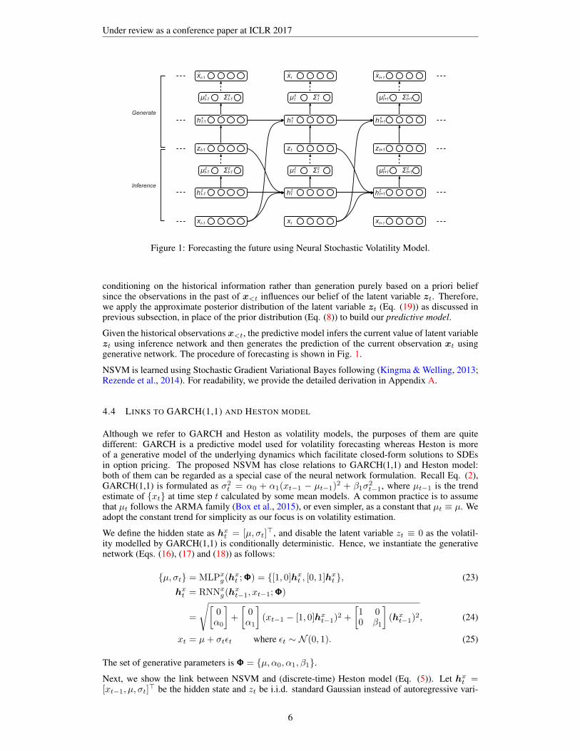
Under review as a conference paper at ICLR 2017

Inference

Generate

xt+1

h t+1x

zt+1

ht+1z

xt+1

xt

h tx

zt

htz

xt

xt-1

h t-1x

zt-1

μt-1z Σt-1

z μ tz Σ t

z μt+1z Σt+1

z

μt-1x Σt-1

x μ tx Σ t

x μt+1x Σt+1

x

ht-1z

xt-1

Figure 1: Forecasting the future using Neural Stochastic Volatility Model.

conditioning on the historical information rather than generation purely based on a priori beliefsince the observations in the past of x<t influences our belief of the latent variable zt. Therefore,we apply the approximate posterior distribution of the latent variable zt (Eq. (19)) as discussed inprevious subsection, in place of the prior distribution (Eq. (8)) to build our predictive model.

Given the historical observations x<t, the predictive model infers the current value of latent variablezt using inference network and then generates the prediction of the current observation xt usinggenerative network. The procedure of forecasting is shown in Fig. 1.

NSVM is learned using Stochastic Gradient Variational Bayes following (Kingma & Welling, 2013;Rezende et al., 2014). For readability, we provide the detailed derivation in Appendix A.

4.4 LINKS TO GARCH(1,1) AND HESTON MODEL

Although we refer to GARCH and Heston as volatility models, the purposes of them are quitedifferent: GARCH is a predictive model used for volatility forecasting whereas Heston is moreof a generative model of the underlying dynamics which facilitate closed-form solutions to SDEsin option pricing. The proposed NSVM has close relations to GARCH(1,1) and Heston model:both of them can be regarded as a special case of the neural network formulation. Recall Eq. (2),GARCH(1,1) is formulated as σ2

t = α0 + α1(xt−1 − µt−1)2 + β1σ

2t−1, where µt−1 is the trend

estimate of {xt} at time step t calculated by some mean models. A common practice is to assumethat µt follows the ARMA family (Box et al., 2015), or even simpler, as a constant that µt ≡ µ. Weadopt the constant trend for simplicity as our focus is on volatility estimation.

We define the hidden state as hxt = [µ, σt]

>, and disable the latent variable zt ≡ 0 as the volatil-ity modelled by GARCH(1,1) is conditionally deterministic. Hence, we instantiate the generativenetwork (Eqs. (16), (17) and (18)) as follows:

{µ, σt} = MLPxg(h

xt ;Φ) = {[1, 0]hx

t , [0, 1]hxt }, (23)

hxt = RNNx

g(hxt−1, xt−1;Φ)

=

√[0α0

]+

[0α1

](xt−1 − [1, 0]hx

t−1)2 +

[1 00 β1

](hx

t−1)2, (24)

xt = µ+ σtεt where εt ∼ N (0, 1). (25)

The set of generative parameters is Φ = {µ, α0, α1, β1}.Next, we show the link between NSVM and (discrete-time) Heston model (Eq. (5)). Let hx

t =[xt−1, µ, σt]

> be the hidden state and zt be i.i.d. standard Gaussian instead of autoregressive vari-

6

Under review as a conference paper at ICLR 2017

able, we represent the Heston model in the framework of NSVM as:[εtzt

]= N (0,

[1 ρρ 1

]), (26)

{µt, σt} = MLPxg(h

xt ;Φ) = {[1, 1, 0]hx

t − [0, 0, 0.5](hxt )

2, [0, 0, 1]hxt }, (27)

hxt = RNNx

g(hxt−1, xt−1, zt;Φ)

=

[0 0 00 1 00 0 1 + a

]hxt−1 +

[100

]xt−1 +

[00b

]zt, (28)

xt = µt + σtεt. (29)

The set of generative parameters is Φ = {µ, a, b}.One should notice that, in practice, the formulation may change in accordance with the specific ar-chitecture of neural networks involved in building the model, and hence a closed-form representationmay be absent.

5 EXPERIMENTS

In this section, we present our experiments1 both on the synthetic and real-world datasets to validatethe effectiveness of NSVM.

5.1 BASELINES AND EVALUATION METRICS

To evaluate the performance of volatility modelling, we adopt the standard economet-ric model GARCH(1,1) Bollerslev (1986) as well as its variants EGARCH(1,1) Nelson(1991), GJR-GARCH(1,1,1) Glosten et al. (1993), ARCH(5), TARCH(1,1,1), APARCH(1,1,1),AGARCH(1,1,1), NAGARCH(1,1,1), IGARCH(1,1), IAVGARCH(1,1), FIGARCH(1,d,1) as base-lines, which incorporate with the corresponding mean model AR(20). We would also compare ourNSVM against a MCMC-based model “stochvol” and the recent Gaussian-processes-based model“GPVOL” Wu et al. (2014), which is a non-parametric model jointly learning the dynamics andhidden states via online inference algorithm. In addition, we setup a naive forecasting model as analternative baseline referred to as NAIVE, which maintains a sliding window of size 20 on the mostrecent historical observations and forecasts the current values of mean and volatility by the averagemean and variance of the window.

For synthetic data experiments, we take four metrics into consideration for performance evaluation:1) the negative log-likelihood (NLL) of observing the test sequence with respect to the generativemodel parameters; 2) the mean-squared error (MSE) between the predicted mean and the groundtruth (µ-MSE), 3) MSE of the predicted variance against the true variance (σ-MSE); 4) smoothnessof fit, which is the standard deviation of the differences of succesive variance estimates. As for thereal-world scenarios, the trend and volatility are implicit such that no ground truth is accessible tocompare with, we consider only NLL and smoothness as the metrics for evaluation on real-worlddata experiment.

5.2 MODEL IMPLEMENTATION

The implementation of NSVM in experiments is in accordance with the architecture illustrated inFig. 1: it consists of two neural networks, namely inference network and generative network. Eachnetwork comprises a set of RNN/MLP as we have discussed above: the RNN is instantiated bystacked LSTM layers whereas the MLP is essentially a 1-layer fully-connected feedforward networkwhich splits into two equal-sized sublayers with different activation functions – one sublayer appliesexponential function to impose the non-negativity and prevents overshooting of variance estimateswhile the other uses linear function to calculate mean estimates. During experiment, the model isstructured by cascading the inference network and generative network as depicted in Fig. 1. Theinput layer is of size 20, which is the same as the embedding dimension DE ; the layer on the

1Repeatable experiment code: https://github.com/xxj96/nsvm

7

Under review as a conference paper at ICLR 2017

interface of inference network and generative network – we call it latent variable layer – representsthe latent variable z, where its dimension is 2. The output layer has the same structure as the inputone, therefore the latent variable layer acts as a bottleneck of the entire architecture which helps toextract the key factor. The stacked layers between input layer, latent variable layer and output layerare the hidden layers of either inference network or generative network, it consists of 1 or 2 LSTMlayers with size 10, which contains recurrent connection for temporal dependencies modelling.

State-of-the-art learning techniques have been applied: we introduce Dropout (Zaremba et al., 2014)into each LSTM recurrent layer and impose L2-norm on the weights of each fully-connected feed-forward layer as regularistion; NADAM optimiser (Dozat, 2015) is exploited for fast convergence,which is a variant of ADAM optimiser (Kingma & Ba, 2014) incorporated with Nesterov momen-tum; stepwise exponential learning rate decay is adopted to anneal the variations of convergence astime goes.

For econometric models, we utilise several widely-used packages for time series analysis: statsmod-els (http://statsmodels.sourceforge.net/), arch (https://pypi.python.org/pypi/arch/3.2), Oxford-MFE-toolbox (https://www.kevinsheppard.com/MFE_Toolbox), stochvol (https://cran.r-project.org/web/packages/stochvol) and fGarch (https://cran.r-project.org/web/packages/fGarch).The implementation of GPVOL is retrived from http://jmhl.org and we adopt the samehyperparameter setting as in Wu et al. (2014).

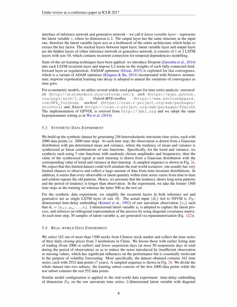
5.3 SYNTHETIC DATA EXPERIMENT

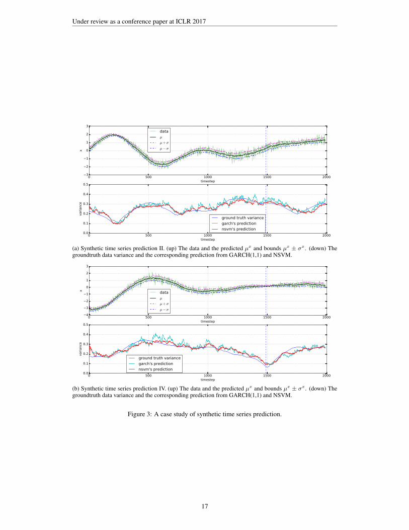
We build up the synthetic dataset by generating 256 heteroskedastic univariate time series, each with2000 data points i.e. 2000 time steps. At each time step, the observation is drawn from a Gaussiandistribution with pre-determined mean and variance, where the tendency of mean and variance issynthesised as linear combinations of sine functions. Specifically, for the trend and variance, wesynthesis each using 3 sine functions with randomly chosen amplitudes and frequencies; then thevalue of the synthesised signal at each timestep is drawn from a Gaussian distribution with thecorresponding value of trend and variance at that timestep. A sampled sequence is shown in Fig. 2a.We expect that this limited dataset could well simulate the real-world scenarios: one usually has verylimited chances to observe and collect a large amount of data from time-invariant distributions. Inaddition, it seems that every observable or latent quantity within time series varies from time to timeand seldom repeats the old patterns. Hence, we presume that the tendency shows long-term patternsand the period of tendency is longer than observation. In the experiment, we take the former 1500time steps as the training set whereas the latter 500 as the test set.

For the synthetic data experiment, we simplify the recurrent layers in both inference net andgenerative net as single LSTM layer of size 10. The actual input {~xt} fed to NSVM is DE-dimensional time-delay embedding (Kennel et al., 1992) of raw univariate observation {xt} suchthat ~xt = [xt+1−DE

, . . . , xt]. 2-dimensional latent variable zt is adopted to capture the latent pro-cess, and enforces an orthogonal representation of the process by using diagonal covariance matrix.At each time step, 30 samples of latent variable zt are generated via reparameterisation (Eq. (22)).

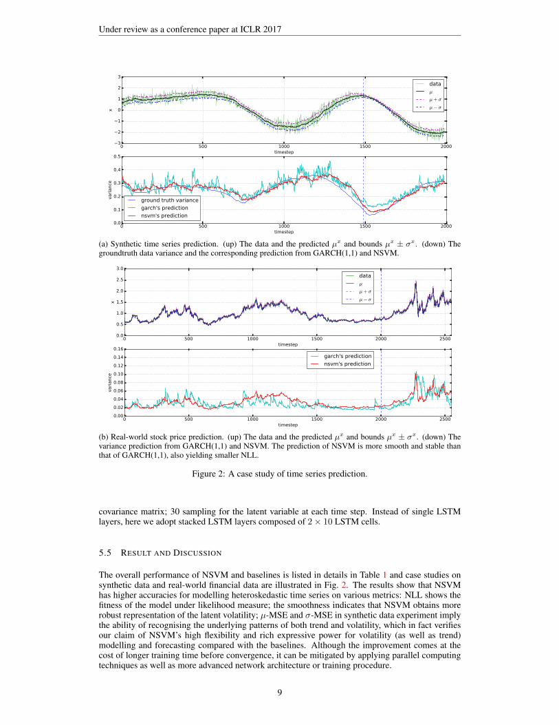
5.4 REAL-WORLD DATA EXPERIMENT

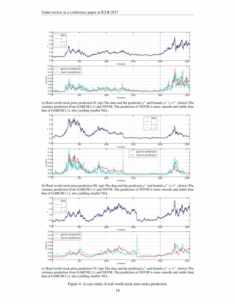
We select 162 out of more than 1500 stocks from Chinese stock market and collect the time seriesof their daily closing prices from 3 institutions in China. We favour those with earlier listing dateof trading (from 2006 or earlier) and fewer suspension days (at most 50 suspension days in totalduring the period of observation) so as to reduce the noise introduced by insufficient observationor missing values, which has significant influences on the performance but is essentially irrelevantto the purpose of volatility forecasting. More specifically, the dataset obtained contains 162 timeseries, each with 2552 data points (7 years). A sampled sequence is shown in Fig. 2b. We divide thewhole dataset into two subsets: the training subset consists of the first 2000 data points while thetest subset contains the rest 552 data points.

Similar model configuration is applied to the real-world data experiment: time-delay embeddingof dimension DE on the raw univariate time series; 2-dimensional latent variable with diagonal

8

Under review as a conference paper at ICLR 2017

0 500 1000 1500 2000timestep

3

2

1

0

1

2

3

x

data

µ

µ+ σ

µ− σ

0 500 1000 1500 2000timestep

0.0

0.1

0.2

0.3

0.4

0.5

vari

ance

ground truth variance

garch's prediction

nsvm's prediction

(a) Synthetic time series prediction. (up) The data and the predicted µx and bounds µx ± σx. (down) Thegroundtruth data variance and the corresponding prediction from GARCH(1,1) and NSVM.

0 500 1000 1500 2000 2500timestep

0.0

0.5

1.0

1.5

2.0

2.5

3.0

x

data

µ

µ+ σ

µ− σ

0 500 1000 1500 2000 2500timestep

0.00

0.02

0.04

0.06

0.08

0.10

0.12

0.14

0.16

vari

ance

garch's prediction

nsvm's prediction

(b) Real-world stock price prediction. (up) The data and the predicted µx and bounds µx ± σx. (down) Thevariance prediction from GARCH(1,1) and NSVM. The prediction of NSVM is more smooth and stable thanthat of GARCH(1,1), also yielding smaller NLL.

Figure 2: A case study of time series prediction.

covariance matrix; 30 sampling for the latent variable at each time step. Instead of single LSTMlayers, here we adopt stacked LSTM layers composed of 2× 10 LSTM cells.

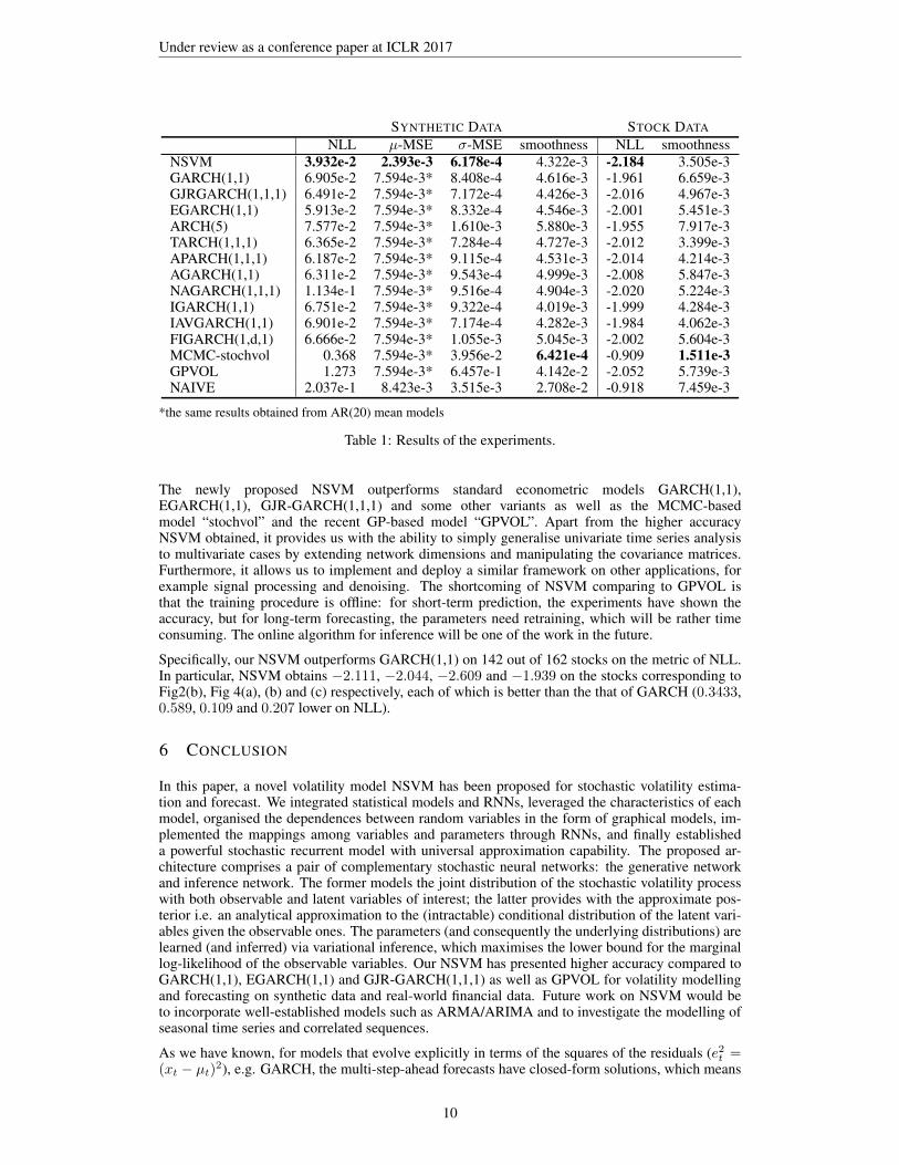
5.5 RESULT AND DISCUSSION

The overall performance of NSVM and baselines is listed in details in Table 1 and case studies onsynthetic data and real-world financial data are illustrated in Fig. 2. The results show that NSVMhas higher accuracies for modelling heteroskedastic time series on various metrics: NLL shows thefitness of the model under likelihood measure; the smoothness indicates that NSVM obtains morerobust representation of the latent volatility; µ-MSE and σ-MSE in synthetic data experiment implythe ability of recognising the underlying patterns of both trend and volatility, which in fact verifiesour claim of NSVM’s high flexibility and rich expressive power for volatility (as well as trend)modelling and forecasting compared with the baselines. Although the improvement comes at thecost of longer training time before convergence, it can be mitigated by applying parallel computingtechniques as well as more advanced network architecture or training procedure.

9

Under review as a conference paper at ICLR 2017

SYNTHETIC DATA STOCK DATA

NLL µ-MSE σ-MSE smoothness NLL smoothnessNSVM 3.932e-2 2.393e-3 6.178e-4 4.322e-3 -2.184 3.505e-3GARCH(1,1) 6.905e-2 7.594e-3* 8.408e-4 4.616e-3 -1.961 6.659e-3GJRGARCH(1,1,1) 6.491e-2 7.594e-3* 7.172e-4 4.426e-3 -2.016 4.967e-3EGARCH(1,1) 5.913e-2 7.594e-3* 8.332e-4 4.546e-3 -2.001 5.451e-3ARCH(5) 7.577e-2 7.594e-3* 1.610e-3 5.880e-3 -1.955 7.917e-3TARCH(1,1,1) 6.365e-2 7.594e-3* 7.284e-4 4.727e-3 -2.012 3.399e-3APARCH(1,1,1) 6.187e-2 7.594e-3* 9.115e-4 4.531e-3 -2.014 4.214e-3AGARCH(1,1) 6.311e-2 7.594e-3* 9.543e-4 4.999e-3 -2.008 5.847e-3NAGARCH(1,1,1) 1.134e-1 7.594e-3* 9.516e-4 4.904e-3 -2.020 5.224e-3IGARCH(1,1) 6.751e-2 7.594e-3* 9.322e-4 4.019e-3 -1.999 4.284e-3IAVGARCH(1,1) 6.901e-2 7.594e-3* 7.174e-4 4.282e-3 -1.984 4.062e-3FIGARCH(1,d,1) 6.666e-2 7.594e-3* 1.055e-3 5.045e-3 -2.002 5.604e-3MCMC-stochvol 0.368 7.594e-3* 3.956e-2 6.421e-4 -0.909 1.511e-3GPVOL 1.273 7.594e-3* 6.457e-1 4.142e-2 -2.052 5.739e-3NAIVE 2.037e-1 8.423e-3 3.515e-3 2.708e-2 -0.918 7.459e-3

*the same results obtained from AR(20) mean models

Table 1: Results of the experiments.

The newly proposed NSVM outperforms standard econometric models GARCH(1,1),EGARCH(1,1), GJR-GARCH(1,1,1) and some other variants as well as the MCMC-basedmodel “stochvol” and the recent GP-based model “GPVOL”. Apart from the higher accuracyNSVM obtained, it provides us with the ability to simply generalise univariate time series analysisto multivariate cases by extending network dimensions and manipulating the covariance matrices.Furthermore, it allows us to implement and deploy a similar framework on other applications, forexample signal processing and denoising. The shortcoming of NSVM comparing to GPVOL isthat the training procedure is offline: for short-term prediction, the experiments have shown theaccuracy, but for long-term forecasting, the parameters need retraining, which will be rather timeconsuming. The online algorithm for inference will be one of the work in the future.

Specifically, our NSVM outperforms GARCH(1,1) on 142 out of 162 stocks on the metric of NLL.In particular, NSVM obtains −2.111, −2.044, −2.609 and −1.939 on the stocks corresponding toFig2(b), Fig 4(a), (b) and (c) respectively, each of which is better than the that of GARCH (0.3433,0.589, 0.109 and 0.207 lower on NLL).

6 CONCLUSION

In this paper, a novel volatility model NSVM has been proposed for stochastic volatility estima-tion and forecast. We integrated statistical models and RNNs, leveraged the characteristics of eachmodel, organised the dependences between random variables in the form of graphical models, im-plemented the mappings among variables and parameters through RNNs, and finally establisheda powerful stochastic recurrent model with universal approximation capability. The proposed ar-chitecture comprises a pair of complementary stochastic neural networks: the generative networkand inference network. The former models the joint distribution of the stochastic volatility processwith both observable and latent variables of interest; the latter provides with the approximate pos-terior i.e. an analytical approximation to the (intractable) conditional distribution of the latent vari-ables given the observable ones. The parameters (and consequently the underlying distributions) arelearned (and inferred) via variational inference, which maximises the lower bound for the marginallog-likelihood of the observable variables. Our NSVM has presented higher accuracy compared toGARCH(1,1), EGARCH(1,1) and GJR-GARCH(1,1,1) as well as GPVOL for volatility modellingand forecasting on synthetic data and real-world financial data. Future work on NSVM would beto incorporate well-established models such as ARMA/ARIMA and to investigate the modelling ofseasonal time series and correlated sequences.

As we have known, for models that evolve explicitly in terms of the squares of the residuals (e2t =(xt − µt)

2), e.g. GARCH, the multi-step-ahead forecasts have closed-form solutions, which means

10

Under review as a conference paper at ICLR 2017

that those forecasts can be efficiently computed in a recursive fashion due to the linear formulationof the model and the exploitation of relation Et−1[e

2t ] = σ2

t .

On the other hand, for models that are not linear or do not explicitly evolve in terms of e2, e.g.EGARCH (linear but not evolve in terms of e2), our NSVM (nonlinear and not evolve in termsof e2), the closed-form solutions are absent and thus the analytical forecast is not available. Wewill instead use simulation-based forecast, which uses random number generator to simulate drawsfrom the predicted distribution and build up a pre-specified number of paths of the variances at 1step ahead. The draws are then averaged to produce the forecast of the next step. For n-step-aheadforecast, it requires n iterations of 1-step-ahead forecast to get there.

NSVM is designed as an end-to-end model for volatility estimation and forecast. It takes the priceof stocks as input and outputs the distribution of the price at next step. It learns the dynamics usingRNN, leading to an implicit, highly nonlinear formulation, where only simulation-based forecast isavailable. In order to obtain reasonably accurate forecasts, the number of draws should be relativelylarge, which will be very expensive for computation. Moreover, the number of draws will increaseexponentially as the forecast horizon grows, so it will be infeasible to forecast several time stepsahead. We have planned to investigate the characteristics of NSVM’s long-horizontal forecasts andtry to design a model specific sampling method for efficient evaluation in the future.

REFERENCES

Torben G Andersen and Tim Bollerslev. Answering the skeptics: Yes, standard volatility models doprovide accurate forecasts. International economic review, pp. 885–905, 1998.

Marco Avellaneda and Antonio Paras. Managing the volatility risk of portfolios of derivative se-curities: the lagrangian uncertain volatility model. Applied Mathematical Finance, 3(1):21–52,1996.

Dzmitry Bahdanau, Kyunghyun Cho, and Yoshua Bengio. Neural machine translation by jointlylearning to align and translate. arXiv preprint arXiv:1409.0473, 2014.

Justin Bayer and Christian Osendorfer. Learning stochastic recurrent networks. arXiv preprintarXiv:1411.7610, 2014.

Christopher M Bishop. Pattern recognition. Machine Learning, 128, 2006.

Tim Bollerslev. Generalized autoregressive conditional heteroskedasticity. Journal of econometrics,31(3):307–327, 1986.

George EP Box, Gwilym M Jenkins, Gregory C Reinsel, and Greta M Ljung. Time series analysis:forecasting and control. John Wiley & Sons, 2015.

Kyunghyun Cho, Bart Van Merrienboer, Caglar Gulcehre, Dzmitry Bahdanau, Fethi Bougares, Hol-ger Schwenk, and Yoshua Bengio. Learning phrase representations using rnn encoder-decoderfor statistical machine translation. arXiv preprint arXiv:1406.1078, 2014.

Jan K Chorowski, Dzmitry Bahdanau, Dmitriy Serdyuk, Kyunghyun Cho, and Yoshua Bengio.Attention-based models for speech recognition. In Advances in Neural Information ProcessingSystems, pp. 577–585, 2015.

Junyoung Chung, Kyle Kastner, Laurent Dinh, Kratarth Goel, Aaron C Courville, and Yoshua Ben-gio. A recurrent latent variable model for sequential data. In Advances in neural informationprocessing systems, pp. 2980–2988, 2015.

John C Cox, Jonathan E Ingersoll Jr, and Stephen A Ross. A theory of the term structure of interestrates. Econometrica: Journal of the Econometric Society, pp. 385–407, 1985.

Timothy Dozat. Incorporating nesterov momentum into adam. 2015.

Robert F Engle. Autoregressive conditional heteroscedasticity with estimates of the variance ofunited kingdom inflation. Econometrica: Journal of the Econometric Society, pp. 987–1007,1982.

11

Under review as a conference paper at ICLR 2017

Robert F Engle and Kenneth F Kroner. Multivariate simultaneous generalized arch. Econometrictheory, 11(01):122–150, 1995.

Otto Fabius and Joost R van Amersfoort. Variational recurrent auto-encoders. arXiv preprintarXiv:1412.6581, 2014.

Marco Fraccaro, Søren Kaae Sønderby, Ulrich Paquet, and Ole Winther. Sequential neural modelswith stochastic layers. arXiv preprint arXiv:1605.07571, 2016.

Lawrence R Glosten, Ravi Jagannathan, and David E Runkle. On the relation between the expectedvalue and the volatility of the nominal excess return on stocks. The journal of finance, 48(5):1779–1801, 1993.

Alex Graves. Generating sequences with recurrent neural networks. arXiv preprintarXiv:1308.0850, 2013.

Alex Graves, Abdel-rahman Mohamed, and Geoffrey Hinton. Speech recognition with deep recur-rent neural networks. In 2013 IEEE international conference on acoustics, speech and signalprocessing, pp. 6645–6649. IEEE, 2013.

Karol Gregor, Ivo Danihelka, Alex Graves, Danilo Jimenez Rezende, and Daan Wierstra. Draw: Arecurrent neural network for image generation. arXiv preprint arXiv:1502.04623, 2015.

Barbara Hammer. On the approximation capability of recurrent neural networks. Neurocomputing,31(1):107–123, 2000.

Kaiming He, Xiangyu Zhang, Shaoqing Ren, and Jian Sun. Deep residual learning for image recog-nition. arXiv preprint arXiv:1512.03385, 2015.

Steven L Heston. A closed-form solution for options with stochastic volatility with applications tobond and currency options. Review of financial studies, 6(2):327–343, 1993.

Geoffrey Hinton, Li Deng, Dong Yu, George E Dahl, Abdel-rahman Mohamed, Navdeep Jaitly,Andrew Senior, Vincent Vanhoucke, Patrick Nguyen, Tara N Sainath, et al. Deep neural networksfor acoustic modeling in speech recognition: The shared views of four research groups. IEEESignal Processing Magazine, 29(6):82–97, 2012.

Sepp Hochreiter and Jurgen Schmidhuber. Long short-term memory. Neural computation, 9(8):1735–1780, 1997.

John C Hull. Options, futures, and other derivatives. Pearson Education India, 2006.

Matthew B Kennel, Reggie Brown, and Henry DI Abarbanel. Determining embedding dimensionfor phase-space reconstruction using a geometrical construction. Physical review A, 45(6):3403,1992.

Diederik Kingma and Jimmy Ba. Adam: A method for stochastic optimization. arXiv preprintarXiv:1412.6980, 2014.

Diederik P Kingma and Max Welling. Auto-encoding variational bayes. arXiv preprintarXiv:1312.6114, 2013.

Alex Krizhevsky, Ilya Sutskever, and Geoffrey E Hinton. Imagenet classification with deep convo-lutional neural networks. In Advances in neural information processing systems, pp. 1097–1105,2012.

Yann LeCun, Yoshua Bengio, and Geoffrey Hinton. Deep learning. Nature, 521(7553):436–444,2015.

Minh-Thang Luong, Hieu Pham, and Christopher D Manning. Effective approaches to attention-based neural machine translation. arXiv preprint arXiv:1508.04025, 2015.

Daniel B Nelson. Conditional heteroskedasticity in asset returns: A new approach. Econometrica:Journal of the Econometric Society, pp. 347–370, 1991.

12

Under review as a conference paper at ICLR 2017

Ser-Huang Poon and Clive WJ Granger. Forecasting volatility in financial markets: A review. Jour-nal of economic literature, 41(2):478–539, 2003.

Danilo Jimenez Rezende, Shakir Mohamed, and Daan Wierstra. Stochastic backpropagation andapproximate inference in deep generative models. arXiv preprint arXiv:1401.4082, 2014.

Jurgen Schmidhuber. Deep learning in neural networks: An overview. Neural Networks, 61:85–117,2015.

Mike Schuster and Kuldip K Paliwal. Bidirectional recurrent neural networks. IEEE Transactionson Signal Processing, 45(11):2673–2681, 1997.

Josef Stoer and Roland Bulirsch. Introduction to numerical analysis, volume 12. Springer Science& Business Media, 2013.

Ilya Sutskever, Oriol Vinyals, and Quoc V Le. Sequence to sequence learning with neural networks.In Advances in neural information processing systems, pp. 3104–3112, 2014.

Aaron van den Oord, Nal Kalchbrenner, and Koray Kavukcuoglu. Pixel recurrent neural networks.arXiv preprint arXiv:1601.06759, 2016.

Yue Wu, Jose Miguel Hernandez-Lobato, and Zoubin Ghahramani. Gaussian process volatilitymodel. In Advances in Neural Information Processing Systems, pp. 1044–1052, 2014.

Wojciech Zaremba, Ilya Sutskever, and Oriol Vinyals. Recurrent neural network regularization.arXiv preprint arXiv:1409.2329, 2014.

13

Under review as a conference paper at ICLR 2017

A COMPLEMENTARY DISCUSSIONS OF NSVM

In this appendix section we present detailed derivations of NSVM, specifically, the parameters learn-ing and calibration, and covariance reparameterisation.

A.1 LEARNING PARAMETERS / CALIBRATION

Given the observationsX , the objective of learning is to maximise the marginal log-likelihood ofXgiven Φ, where the posterior is involved. However, as we have discussed in the previous subsection,the true posterior is usually intractable, which means exact inference is difficult. Hence, approximateinference is applied instead of rather than exact inference by following (Kingma & Welling, 2013;Rezende et al., 2014). We represent the marginal log-likelihood ofX in the following form:

ln pΦ(X) = EqΨ(Z|X)

[lnpΦ(X,Z)

pΦ(Z|X)

]= EqΨ(Z|X)

[lnpΦ(X,Z)

qΨ(Z|X)

qΨ(Z|X)

pΦ(Z|X)

]= EqΨ(Z|X)[ln pΦ(X,Z)− ln qΨ(Z|X)] +KL[qΨ(Z|X)‖pΦ(Z|X)]

≥ EqΨ(Z|X)[ln pΦ(X,Z)− ln qΨ(Z|X)] (as KL ≥ 0), (30)

where the expectation term EqΨ(Z|X)[ln pΦ(X,Z) − ln qΨ(Z|X)] is referred to as the variationallower bound L[q;X,Φ,Ψ] of the approximate posterior qΨ(Z|X,Ψ). The lower bound is essen-tially a functional with respect to distribution q and parameterised by observationsX and parametersets Φ,Ψ of both generative and inference model. In theory, the marginal log-likelihood is max-imised by optimisation on the lower bound L[q;X,Φ,Ψ] with respect to Φ and Ψ.

We apply the factorisations in Eqs. (10) and (19) to the integrand within expectation of Eq. (30):

ln pΦ(X,Z)− ln qΨ(Z|X) =∑t

[lnN (xt;µ

xΦ(x<t, z≤t),Σ

xΦ(x<t, z≤t))

+ lnN (zt;µzΦ(z<t),Σ

zΦ(z<t))− lnN (zt; µ

zΨ(z<t,x<t), Σ

zΨ(z<t,x<t))

]. (31)

As there is usually no closed-form solution for the expecation (Eq. (30)), we have to estimate theexpectation by applying sampling methods to latent variable zt through time in accordance withthe causal dependences. We utilise the reparameterisation of zt as shown in Eq. (22) such thatwe sample the corresponding auxiliary standard variable εt rather than zt itself and compute thevalue of zt on the fly. This ensures that the gradient-based optimisation techniques are applicableas the reparameterisation isolates the model parameters of interest from the sampling procedure. Bysampling N sample paths, the estimator of the lower bound is defined as the average of paths:

L =− 1

2N

∑t

[ln detΣz

t + (µzt + A

zt ε

zt − µz

t )>(Σz

t )−1(µz

t + Azt ε

zt − µz

t )

+ ln detΣxt + (xt − µx

t )>(Σx

t )−1(xt − µx

t )− ln det Σt

]+ const, (32)

where Azt (A

zt )> = Σz

t and εzt ∼ N (0, Iz) is parameter-independent and considered as constantwhen calculating derivatives.

A.2 COVARIANCE PARAMETERISATION

As is known, it entails a computational complexity of O(M3) to maintain and update the full-sizecovariance Σ with M dimensions (Rezende et al., 2014). In the case of very high dimensions, thefull-size covariance matrix would be too computationally expensive to afford. Hence, we use insteadthe covariance matrices with much fewer parameters for efficiency. The simplest setting is to usediagonal precision matrix (i.e. the inverse of covariance matrix) Σ−1 = D. However, it drawsvery strong restrictions on representation of the random variable of interest as the diagonal precisionmatrix (and thus diagonal covariance matrix) indicates independence among the dimensions. There-fore, the tradeoff becomes low-rank perturbation on diagonal matrix: Σ−1 = D + V V >, whereV = {v1, . . . ,vK} denotes the perturbation while each vk is a M -dimensional column vector.

14

Under review as a conference paper at ICLR 2017

The corresponding covariance matrix and its determinant is obtained using Woodbury identity andmatrix determinant lemma:

Σ =D−1 −D−1V (I + V >D−1V )−1V >D−1 (33)

ln detΣ = − ln det (D + V V >) = − ln detD − ln det (I + V >D−1V ) (34)

To calculate the deviation A for the factorisation of covariance matrix Σ = AA>, we first con-sider the rank-1 perturbation where K = 1. It follows that V = v is a column vector, andI + V >D−1V = 1 + v>D−1v is a real number. A particular solution ofA is obtain:

A =D−12 − [γ−1(1−√η)]D−1vv>D− 1

2 (35)

where γ = v>D−1v, η = (1 + γ)−1. The computational complexity involved here is merelyO(M).

Observe that V V > =∑K

k=1 vkv>k , the perturbation of rank K is essentially the superposition of

K perturbations of rank 1. Therefore, we can calculate the deviation A iteratively, an algorithm isprovided to demonstrate the procedure of calculation. The computational complexity for rank-Kperturbation remains to be O(M) given K �M .

Algorithm 1 gives the detailed calculation scheme.

Algorithm 1 Calculation of rank-K perturbation of precision matricesInput: The original diagonal matrixD; The rank-K perturbation V = {v1, . . . ,vK}Output: A such that the factorisationAA> = Σ = (D + V V >)−1 holds

1: A(0) =D− 1

2

2: i = 03: while i < K do4: γ(i) = v

>(i)A(i)A

>(i)v(i)

5: η(i) = (1 + γ(i))−1

6: A(i+1) = A(i) − [γ−1(i) (1−√η(i))]A(i)A

>(i)v(i)v

>(i)A(i)

7: A = A(K)

15

Under review as a conference paper at ICLR 2017

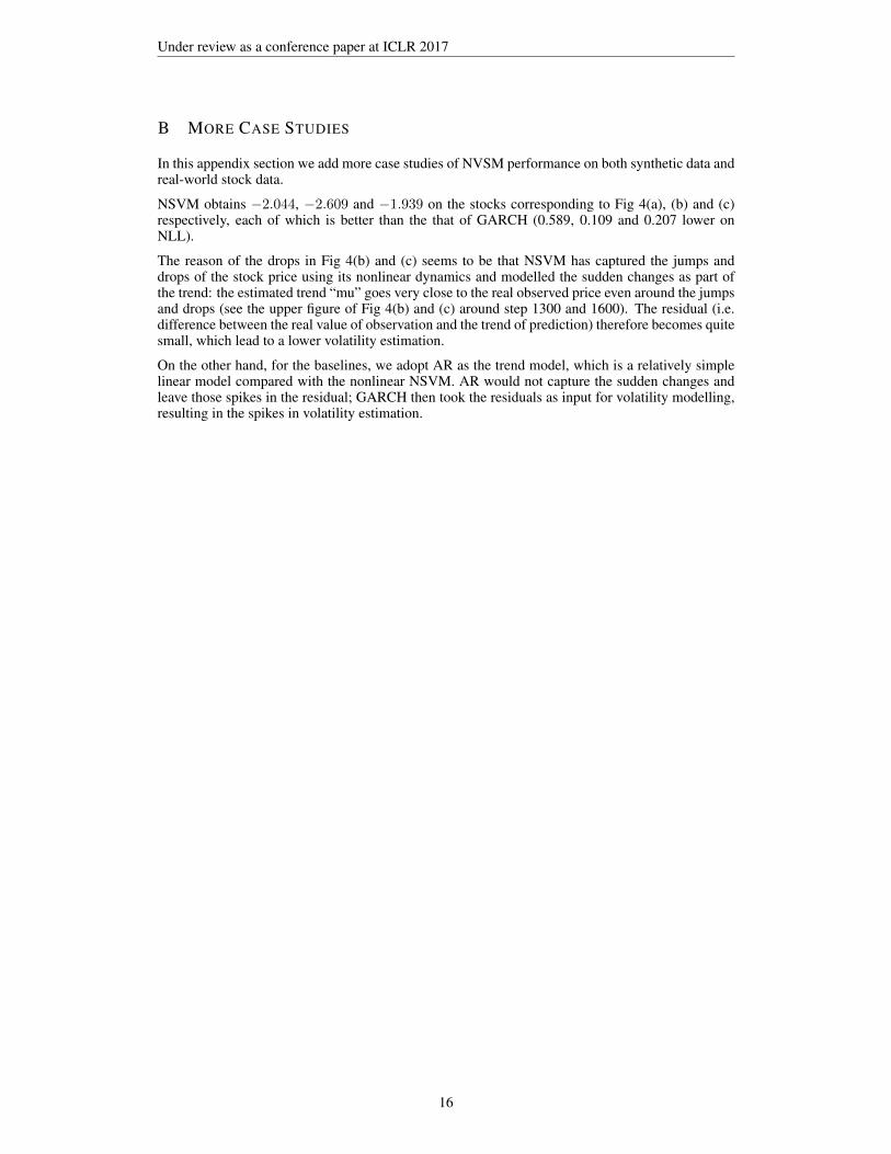
B MORE CASE STUDIES

In this appendix section we add more case studies of NVSM performance on both synthetic data andreal-world stock data.

NSVM obtains −2.044, −2.609 and −1.939 on the stocks corresponding to Fig 4(a), (b) and (c)respectively, each of which is better than the that of GARCH (0.589, 0.109 and 0.207 lower onNLL).

The reason of the drops in Fig 4(b) and (c) seems to be that NSVM has captured the jumps anddrops of the stock price using its nonlinear dynamics and modelled the sudden changes as part ofthe trend: the estimated trend “mu” goes very close to the real observed price even around the jumpsand drops (see the upper figure of Fig 4(b) and (c) around step 1300 and 1600). The residual (i.e.difference between the real value of observation and the trend of prediction) therefore becomes quitesmall, which lead to a lower volatility estimation.

On the other hand, for the baselines, we adopt AR as the trend model, which is a relatively simplelinear model compared with the nonlinear NSVM. AR would not capture the sudden changes andleave those spikes in the residual; GARCH then took the residuals as input for volatility modelling,resulting in the spikes in volatility estimation.

16

Under review as a conference paper at ICLR 2017

0 500 1000 1500 2000timestep

3

2

1

0

1

2

3

x

data

µ

µ+ σ

µ− σ

0 500 1000 1500 2000timestep

0.0

0.1

0.2

0.3

0.4

0.5

vari

ance

ground truth variance

garch's prediction

nsvm's prediction

(a) Synthetic time series prediction II. (up) The data and the predicted µx and bounds µx ± σx. (down) Thegroundtruth data variance and the corresponding prediction from GARCH(1,1) and NSVM.

0 500 1000 1500 2000timestep

4

3

2

1

0

1

2

3

x data

µ

µ+ σ

µ− σ

0 500 1000 1500 2000timestep

0.0

0.1

0.2

0.3

0.4

0.5

vari

ance

ground truth variance

garch's prediction

nsvm's prediction

(b) Synthetic time series prediction IV. (up) The data and the predicted µx and bounds µx ± σx. (down) Thegroundtruth data variance and the corresponding prediction from GARCH(1,1) and NSVM.

Figure 3: A case study of synthetic time series prediction.

17

Under review as a conference paper at ICLR 2017

0 500 1000 1500 2000 2500timestep

0.0

0.5

1.0

1.5

2.0

2.5

3.0

3.5

x

data

µ

µ+ σ

µ− σ

0 500 1000 1500 2000 2500timestep

0.00

0.02

0.04

0.06

0.08

0.10

0.12

0.14

0.16

0.18

vari

ance

garch's prediction

nsvm's prediction

(a) Real-world stock price prediction II. (up) The data and the predicted µx and bounds µx ± σx. (down) Thevariance prediction from GARCH(1,1) and NSVM. The prediction of NSVM is more smooth and stable thanthat of GARCH(1,1), also yielding smaller NLL.

0 500 1000 1500 2000 2500timestep

0.0

0.5

1.0

1.5

2.0

2.5

3.0

x

data

µ

µ+ σ

µ− σ

0 500 1000 1500 2000 2500timestep

0.00

0.02

0.04

0.06

0.08

0.10

0.12

0.14

0.16

vari

ance

garch's prediction

nsvm's prediction

(b) Real-world stock price prediction III. (up) The data and the predicted µx and bounds µx ± σx. (down) Thevariance prediction from GARCH(1,1) and NSVM. The prediction of NSVM is more smooth and stable thanthat of GARCH(1,1), also yielding smaller NLL.

0 500 1000 1500 2000 2500timestep

0.0

0.5

1.0

1.5

2.0

2.5

x

data

µ

µ+ σ

µ− σ

0 500 1000 1500 2000 2500timestep

0.00

0.02

0.04

0.06

0.08

0.10

0.12

0.14

0.16

vari

ance

garch's prediction

nsvm's prediction

(c) Real-world stock price prediction IV. (up) The data and the predicted µx and bounds µx ± σx. (down) Thevariance prediction from GARCH(1,1) and NSVM. The prediction of NSVM is more smooth and stable thanthat of GARCH(1,1), also yielding smaller NLL.

Figure 4: A case study of real-world stock time series prediction.

18